Optimization of cooling load in quantum self-contained fridge based on endoreversible approach

Abstract

We consider a quantum self-contained fridge consisting of three qubits interacting with three separate heat reservoirs, respectively, and functioning without any external controls. Applying the methods of endoreversible thermodynamics, we derive explicit expressions of cooling load versus efficiency of this fridge, which demonstrate behaviors of trade-off between those two quantities and thus enable to discuss the thermoeconomic optimization of performance. We also discuss a possibility for the amplification of cooling load briefly in a simple modification from the original architecture of fridge.

1 Introduction

The issue of cooling has become a considerably important subject in response to the arguable prediction that continued greenhouse gas emissions at the current rate would give rise to further warming and then many significant changes in the global climate system in future IPC07 . Numerous cooling mechanisms and techniques have been developed so far in different industrial systems of refrigeration HAN12 . As an underlying formalism of those mechanisms, a fridge driven by three heat reservoirs, without any extra work sources, has been extensively studied AND83 ; SIE90 . In fact, this architecture of fridge has attracted widespread industrial interest due to its own potential that various forms of low-quality energy such as the waste heat produced in industrial and biological processes could be practically used as driving sources of refrigeration (“energy harvesting”).

The methods of finite-time thermodynamics have been applied to non-equilibrium thermodynamic processes observed in fridge formalisms AND83 ; SIE90 . They have been able to determine the performance bounds and optimal paths of those processes, primarily in terms of cooling load corresponding to output power of work-producing engines, in the context of optimized energy management SIE94 ; CWU96 ; BER99 ; SAH99 ; KOD03 ; QIN05 . Also, as a model of describing non-equilibrium processes, endoreversible thermodynamics has been typically applied to a fridge in such a way that its working substance is operated reversibly (“infinitely” slowly) by an external driving in the Carnot limit while it interacts with heat reservoirs by exchanging heat irreversibly. Therefore, this model is highly useful for performance study of the three-reservoir fridges operating at (real) finite rates.

A big challenge in thermodynamics has arisen with the miniaturization of devices achieved from the remarkable advancement of technology, particularly in the low-temperature regime, where quantum effects are dominant (“quantum thermodynamics”) and the cooling mechanism is a significant issue for high-level performance of quantum devices MAH04 . While most of other proposals for nanoscale quantum fridges have been made to be driven by external controls (being, however, highly nontrivial to implement experimentally with required precision), on the other hand the so-called “self-contained” fridge is operating, remarkably, merely by incoherent interactions with three heat reservoirs at different temperatures LIN10 ; POP10 ; SKR11 ; BRU12 ; CHE12 ; MAT10 , thus being similar to the aforementioned classical model of three-bath fridges in terms of the underlying formalism. Also, it has been found that this quantum model is universal in its efficiency (“coefficient of performance”), depending, i.e., upon the temperatures of baths only, but not upon any other details such as the coupling strengths between system and bath, notably at both the well-known Carnot limit and being away from it BRU12 .

Motivated by this formal similarity, it is interesting to compare both external-work-free fridges (classical and quantal) and apply the endoreversible approach also to this quantum model in order to look into the finite-time thermodynamic aspects therein, which have not yet been discussed extensively. In this paper we intend to investigate, specifically, the cooling load versus coefficient of performance (COP), and its optimization of the quantum self-contained fridge, as well as some relevant issues, which would provide a foundational guidance for performance enhancement in different types of nanoscale fridges, and thus insights into the fundamental mechanism of overcoming various drawbacks observed in the cooling methods at macroscopic level.

The general layout of this paper is the following. In Sect. 2 we briefly review the characteristics of quantum self-contained fridge, needed for our discussion. In Sect. 3 we derive an explicit expression of cooling load versus COP, which enables to discuss the thermoeconomic optimization of performance. In Sect. 4 we discuss the cooling load versus a design parameter characterizing the fridge architecture. We also take into consideration a simple modification of fridge architecture in order to explore a possibility of the amplification of cooling load. Finally we give the concluding remarks of this paper in Sect. 5.

2 Characteristics of self-contained fridge

The system under consideration consists of three qubits, whose energy spacings are given by $E_{a}$, $E_{b}$, and $E_{c}=E_{b}-E_{a}$, respectively, on the assumption that $E_{a}<E_{b}$ (cf. Fig. 1). We are interested in building a cooling machine by merely contacting the three qubits one-on-one to three separate heat baths at different temperatures, initially prepared as ($T_{1},T_{2},T_{3}$) with $T_{1}>T_{2}>T_{3}$; thereby the “hot” bath ${\mathcal{B}}_{1}$ at $T_{1}$ provides heat $Q_{1}$ into this system which can then extracts heat $Q_{3}$ steadily from the “cold” bath ${\mathcal{B}}_{3}$ at $T_{3}$. From BRU12 , it is true that such a system can function as a fridge only when the “biggest” qubit with $E_{b}$ is in contact with the “intermediate” bath ${\mathcal{B}}_{2}$ at $T_{2}$. Therefore, from now on, let the qubits denoted by ($E_{1},E_{2},E_{3}$), with $E_{1}<E_{2}$ and $E_{3}=E_{2}-E_{1}$, be in contact with baths (${\mathcal{B}}_{1},{\mathcal{B}}_{2},{\mathcal{B}}_{3}$), respectively. Moreover, let each qubit $E_{j}$ be initially in equilibrium with ${\mathcal{B}}_{j}$, before the actual cooling process occurs. And we introduce the ratio of energy spacing, $\alpha=E_{1}/E_{2}<1$ as a design parameter characterizing the fridge architecture.

By construction that no extra work is put into the system for driving, its total energy remains unchanged during the cooling process, and it is only possible to observe energy exchanges between the same energy levels inside that system. To make it function as a fridge indeed, it is simply required that before both qubits $E_{1}$ and $E_{2}$ interact with qubit $E_{3}$ to be cooled, the condition $P(0,1,0)<P(1,0,1)$ be met LIN10 . Here, $P(0,1,0)$ denotes the probability of $E_{1}$ being in its ground state, $E_{2}$ being in its excited state, and $E_{3}$ being in its ground state, as well as the probability $P(1,0,1)$ follows similarly. This is equivalent to $e^{-E_{2}/T_{2}}<e^{-E_{1}/T_{1}}\cdot e^{-E_{3}/T_{3}}$ (with $k_{\mbox{\tiny B}}=1$), which will easily reduce to the inequality $T_{3}>T_{v}>0$, expressed in terms of the virtual temperature BRU12

$$T_{v}\,=\,\frac{1-\alpha}{1/T_{2}-\alpha/T_{1}}\,,$$ (1)

being independent of $T_{3}$. Therefore, as long as this inequality condition is met, the fridge functions. Fig. 2 demonstrates the behaviors of $T_{v}$ versus $\alpha$.

It has been shown POP10 ; SKR11 that each of heat exchanged between qubit and bath satisfies in the steady-state the ratio

$$Q_{1}:Q_{2}:Q_{3}\;=\;E_{1}:E_{2}:E_{3}\,.$$ (2)

The COP of this quantum fridge then equals BRU12

$$\eta_{\mbox{\scriptsize fr}}^{(q)}\;:=\;\frac{Q_{3}}{Q_{1}}\;=\;\frac{E_{3}}{E_{1}}\;=\;\frac{T_{2}^{-1}-T_{1}^{-1}}{T_{v}^{-1}-T_{2}^{-1}}\,.$$ (3)

In comparison, the well-known Carnot value $\eta_{\mbox{\tiny C}}$ is given by (3) with $T_{v}\to T_{3}$, which is valid for the classical three-bath fridges as well; note that the value $\eta_{\mbox{\tiny C}}$ of fridges may be greater than unity. Similarly, by replacing $T_{v}$ by $T_{3}$ in (1) and solving for $\alpha$, we can obtain the Carnot value

$$\alpha_{\mbox{\tiny C}}\;=\;\frac{T_{3}^{-1}-T_{2}^{-1}}{T_{3}^{-1}-T_{1}^{-1}}<1\,.$$ (4)

Therefore, only the region of $\alpha_{\mbox{\tiny C}}<\alpha<1$ is allowed for cooling process, as shown in Fig. 2. At the minimum $\alpha_{\mbox{\tiny C}}$, the fridge in fact stops functioning (in the frame of finite-time thermodynamics) due to the fact that $T_{3}\ngtr T_{v}$. It is noted in (4) that with $T_{3}$ becoming lower, the working region of $\alpha$ shrinks. Also, if $T_{2}\to T_{3}$, then $\eta_{\mbox{\tiny C}}\to\infty$ and $\alpha_{\mbox{\tiny C}}\to 0^{+}$, equivalent to $E_{1}\to 0$, which implies the breakdown of this cooling system.

We should pay special attention to the case of $\alpha=1/2$, in which an additional channel of heat transport is open, i.e., a direct heat flow from $E_{1}$ to $E_{3}$ due to the fact that $T_{1}>T_{3}$, being not available at all when $\alpha\neq 1/2$. This is in fact a heat flow in the opposite direction to the cooling process. Therefore, in this case, we need an extra check-up for bringing the overall cooling process true: Since heat flux from one side to the other one is proportional to temperature difference between both sides (cf. details in Sect. 3), it is required that the temperature difference $T_{3}-T_{v}$ for cooling be greater than $T_{1}-T_{3}$ (on the assumption that heat conductances in both directions are the same). This condition easily reduces to the inequality, $0>T_{1}^{2}-2\,T_{3}\,T_{1}+T_{2}\,T_{3}:=f(T_{1})$, being quadratic in $T_{1}$. However, the discriminant of $f(T_{1})$, given by $D=4\,T_{3}\,(T_{3}-T_{2})<0$, indicates that $0\ngtr f(T_{1})$ indeed for all $T_{1}$. As a result, this system cannot function as a fridge at $\alpha=1/2$, in addition to $\alpha=0,1$.

We close this section by reminding that when the actual cooling proceeds, each qubit $E_{j}$ is not in equilibrium with ${\mathcal{B}}_{j}$ any longer, thus being not at $T_{j}$.

3 Cooling load versus fridge efficiency

We first consider a classical model of fridge driven by three heat baths. By applying the first law of thermodynamics to its cyclic process in the (non-equilibrium) steady-state, we easily obtain

$$Q_{1}-Q_{2}+Q_{3}\,=\,0\,.$$ (5)

All of irreversibility during the cooling process may be split into two parts KOD03 ; one is the external irreversibility occurring in (system-bath) heat exchange, resulting from the temperature differences between baths and working substance of the fridge, while the other is the internal irreversibility resulting from all entropy-producing dissipations inside the working substance, say, friction, mass transfer, etc. By applying the second law to the working substance, we obtain

$$\frac{Q_{1}}{T_{i1}}-\frac{Q_{2}}{T_{i2}}+\frac{Q_{3}}{T_{i3}}\,\geq\,0\,,$$ (6)

where the symbol $T_{ij}$ with $j=1,2,3$ denotes internal effective temperature of the working substance’s subsystem being in direct interaction with bath ${\mathcal{B}}_{j}$. Here, the condition of external irreversibility requires that $T_{i1}<T_{1}$, and $T_{i2}>T_{2}$, as well as $T_{i3}<T_{3}$. To simplify our discussion, we apply endoreversible thermodynamics to (6) by neglecting the internal irreversibility, thus the inequality (6) reducing to the equality

$$\frac{Q_{1}}{T_{i1}}-\frac{Q_{2}}{T_{i2}}+\frac{Q_{3}}{T_{i3}}\,=\,0\,,$$ (6a)

which will be in consideration from now on. Combining (5) and (6a) then allows us to have the equality of fridge efficiency (COP)

$$\eta_{\mbox{\scriptsize fr}}\,=\,\frac{Q_{3}}{Q_{1}}\,=\,\frac{T_{i2}^{-1}-T_{i1}^{-1}}{T_{i3}^{-1}-T_{i2}^{-1}}\,.$$ (7)

If heat exchange is carried out infinitely slowly, then the steady-state reduces to the quasi-static state with $T_{j}\leftarrow T_{ij}$ and so the Carnot value $\eta_{\mbox{\tiny C}}\leftarrow\eta_{\mbox{\scriptsize fr}}$. We will below apply those results of endoreversible thermodynamics to the quantum self-contained fridge, say, by identifying $\eta_{\mbox{\scriptsize fr}}^{(q)}$ with (7). In fact, this does not any harm since this quantum fridge already has no source of internal irreversibility at all, due to its architecture.

As a quantity of finite-time thermodynamics, heat flux is now considered during the cooling process, given by $\dot{Q}=k\,(T_{h}-T_{l})$ obeying the Newtonian linear law, in which $k$ denotes a heat conductance, as well as $T_{h}$ and $T_{l}$ are high and low temperatures, respectively SIE90 . From this, it follows that $\dot{Q}_{1}=k_{1}\,(T_{1}-T_{i1})$, and $\dot{Q}_{2}=k_{2}\,(T_{i2}-T_{2})$, as well as $\dot{Q}_{3}=k_{3}\,(T_{3}-T_{i3})$. We now introduce the specific cooling load for the quantum fridge as

$${\mathcal{L}}_{3}:=\dot{Q}_{3}/K\,,$$ (8)

where the total heat conductance $K=k_{1}+k_{2}+k_{3}$. Then it is straightforward to transform (8) into

$${\mathcal{L}}_{3}=\left(\frac{\dot{Q}_{1}}{\dot{Q}_{3}}\,\frac{1}{T_{1}-T_{i1}}+\frac{\dot{Q}_{2}}{\dot{Q}_{3}}\,\frac{1}{T_{i2}-T_{2}}+\frac{1}{T_{3}-T_{i3}}\right)^{-1}$$ (9)

which, with the aid of (5) and (7), reduces to

$${\mathcal{L}}_{3}(\eta_{\mbox{\scriptsize fr}})=\left\{\frac{1}{\eta_{\mbox{\scriptsize fr}}\,(T_{1}-T_{i1})}+\frac{(1/\eta_{\mbox{\scriptsize fr}})+1}{T_{i2}-T_{2}}+\frac{1}{T_{3}-T_{i3}}\right\}^{-1}\,,$$ (10)

then interpreted as a function of a given COP $\eta_{\mbox{\scriptsize fr}}$.

Now we are interested in optimizing this expression of specific cooling load in order to see its steady-state behaviors. Therefore we consider

$$\tilde{\mathcal{L}}_{3}\,=\,{\mathcal{L}}_{3}+\lambda\,\left(\eta_{\mbox{\scriptsize fr}}-\frac{y-x}{1-y}\right)\,,$$ (11)

where $\lambda$ is a Lagrangian multiplier, as well as $x:=T_{i3}/T_{i1}$ and $y:=T_{i3}/T_{i2}$. By requiring that $\partial\tilde{\mathcal{L}}_{3}/\partial x=0$, and $\partial\tilde{\mathcal{L}}_{3}/\partial y=0$, as well as $\partial\tilde{\mathcal{L}}_{3}/\partial T_{i3}=0$, followed by algebraic manipulation, we can determine the optimized values of three effective temperatures as

$$T_{i1} = \frac{1}{2}\,\left\{T_{1}\,+\,\frac{T_{2}\,(1+\eta_{\mbox{\scriptsize fr}}\cdot T_{1}/T_{3})}{1+\eta_{\mbox{\scriptsize fr}}}\right\}$$ (12a)

$$T_{i2} = \frac{1}{2}\,\left\{T_{2}\,+\,\frac{T_{3}\,(1+\eta_{\mbox{\scriptsize fr}})}{T_{3}/T_{1}+\eta_{\mbox{\scriptsize fr}}}\right\}$$ (12b)

$$T_{i3} = \frac{1}{2}\,\left\{T_{3}\,+\,\frac{T_{2}\,(T_{3}/T_{1}+\eta_{\mbox{\scriptsize fr}})}{1+\eta_{\mbox{\scriptsize fr}}}\right\}\,,$$ (12c)

expressed in terms of three given bath temperatures and a given COP only. Substituting (12a)-(12c) into (10), we can finally obtain

$${\mathcal{L}}_{3}(\eta_{\mbox{\scriptsize fr}})\,=\,\frac{T_{2}}{4\,(1+\eta_{\mbox{\scriptsize fr}})}\,-\,\frac{T_{3}}{4\,(1+\eta_{\mbox{\scriptsize fr}}\cdot T_{1}/T_{3})}\,-\,\frac{(T_{2}-T_{3})}{4}\,.$$ (13)

It is easy to confirm that ${\mathcal{L}}_{3}(\eta_{\mbox{\tiny C}})=0$ and ${\mathcal{L}}_{3}(0)=0$ indeed, as required. Further, requiring $\partial{\mathcal{L}}_{3}/\partial\eta_{\mbox{\scriptsize fr}}=0$ will give the maximum value of (13),

$${\mathcal{L}}_{m}\;=\;\frac{(\sqrt{T_{1}\,T_{2}}-T_{3})^{2}}{4\,(T_{1}-T_{3})}-\frac{(T_{2}-T_{3})}{4}\,,$$ (14)

evaluated at $\eta_{m}=(1-\sqrt{T_{2}/T_{1}})/(\sqrt{T_{1}\,T_{2}}/T_{3}-1)$. Fig. 3 demonstrates behaviors of the specific cooling load versus COP for various ($T_{1},T_{2},T_{3}$); here we may regard ${\mathcal{L}}_{3}/{\mathcal{L}}_{m}$ as a measure of irreversibility.

Next, with the help of (12a)-(12c), the heat fluxes can be determined as

$$\dot{Q}_{1}\,=\,\frac{k_{1}\,A}{2\,(1+\eta_{\mbox{\scriptsize fr}})} \dot{Q}_{2}\,=\,\frac{k_{2}\,(T_{3}/T_{1})\,A}{2\,(T_{3}/T_{1}+\eta_{\mbox{\scriptsize fr}})}$$ , (15a)

$$\dot{Q}_{3} = \frac{k_{3}\,(T_{3}/T_{1})\,A}{2\,(1+\eta_{\mbox{\scriptsize fr}})}\,,$$ (15b)

where $A:=T_{1}-T_{2}-\eta_{\mbox{\scriptsize fr}}\,(T_{2}-T_{3})\,T_{1}/T_{3}$. Now we require that the heat conductances satisfy

$$k_{2}/k_{1}=1+\eta_{\mbox{\scriptsize fr}}\,T_{1}/T_{3}\;\;,\;\;k_{3}/k_{1}=\eta_{\mbox{\scriptsize fr}}\,T_{1}/T_{3}\,.$$ (16)

This will immediately yield

$$\dot{Q}_{1}=\dot{Q}_{2}/(1+\eta_{\mbox{\scriptsize fr}})\;\;,\;\;\dot{Q}_{3}=\dot{Q}_{2}\,\eta_{\mbox{\scriptsize fr}}/(1+\eta_{\mbox{\scriptsize fr}})\,,$$ (17)

and $\dot{Q}_{2}=k_{2}\,(A/2)\,(1+\eta_{\mbox{\scriptsize fr}}\,T_{1}/T_{3})^{-1}$ with $k_{2}\propto E_{2}$. With the help of (3), it is then easy to show that Eq. (17) consists with (2) indeed. It is stressed again that heat conductances ($k_{1},k_{2},k_{3}$) in the steady state can be uniquely determined (up to constant) for a given COP and the initial conditions, ($T_{1},T_{2},T_{3}$) and ($E_{1},E_{2}$). Fig. 4 shows behaviors of the heat fluxes $(\dot{Q}_{1},\dot{Q}_{2},\dot{Q}_{3})$ versus COP.

In comparison, we consider the remaining specific heat loads, ${\mathcal{L}}_{1}=\dot{Q}_{1}/K$ and ${\mathcal{L}}_{2}=\dot{Q}_{2}/K$. Along the same lines as applied above for ${\mathcal{L}}_{3}(\eta_{\mbox{\scriptsize fr}})$, it is straightforward to obtain ${\mathcal{L}}_{1}(\eta_{\mbox{\scriptsize fr}})={\mathcal{L}}_{3}/\eta_{\mbox{\scriptsize fr}}$ and ${\mathcal{L}}_{2}(\eta_{\mbox{\scriptsize fr}})={\mathcal{L}}_{3}\cdot(1+\eta_{\mbox{\scriptsize fr}})/\eta_{\mbox{\scriptsize fr}}$, with the same optimized values of effective temperatures as given in (12a)-(12c). Then, both of heat loads will yield exactly the same behaviors of $(\dot{Q}_{1},\dot{Q}_{2},\dot{Q}_{3})$ as those derived from ${\mathcal{L}}_{3}(\eta_{\mbox{\scriptsize fr}})$, shown in Fig. 4. This fact is no surprise since the optimization process in (11) was taken into consideration in order to find uniquely the steady-state behaviors of heat fluxes.

It is also instructive to apply to this quantum fridge the thermoeconomic criterion introduced in SAH99 , then given by

$${\mathcal{F}}_{c}\;:=\;\frac{\dot{Q}_{3}}{C_{t}}\;=\;(a\,\eta_{\mbox{\scriptsize fr}}^{-1}+b\,{\mathcal{L}}_{3}^{-1})^{-1}\,.$$ (18)

Here the total cost $C_{t}$ consists of both energy consumption cost $C_{e}=a\,\dot{Q}_{1}$ and investment cost $C_{i}=b\,K(E_{1},E_{2},E_{3})$ being assumed to be linearly proportional to the system size $E_{j}$ each, with proportionality coefficients $a$ and $b$; e.g., in case of the waste heat in industry to be used as the input energy for fridges, then $C_{e}\ll C_{i}$. The case of $a=0$ and $b=1$ gives ${\mathcal{F}}_{c}\to{\mathcal{L}}_{3}$ while the opposite case of $a=1$ and $b=0$, on the other hand, gives ${\mathcal{F}}_{c}\to\eta_{\mbox{\scriptsize fr}}$. This behavior shows a trade-off between ${\mathcal{L}}_{3}$ and $\eta_{\mbox{\scriptsize fr}}$ in the context of thermoeconomics. By substituting (13) into (18), we can observe those behaviors of ${\mathcal{F}}_{c}(\eta_{\mbox{\scriptsize fr}})$ for various values of $a$ and $b$, as demonstrated in Fig. 5.

Moreover, we note that the total COP in (7) may be rewritten as $\eta_{\mbox{\scriptsize he}}^{(1,2)}\,\eta_{\mbox{\scriptsize fr}}^{(2,3)}$ (cf. SKR11 ), in which both efficiencies are explicitly given by $\eta_{\mbox{\scriptsize he}}^{(1,2)}=(T_{i1}-T_{i2})/T_{i1}$ of an endoreversible heat engine ($E_{1},E_{2}$) and $\eta_{\mbox{\scriptsize fr}}^{(2,3)}=T_{i3}/(T_{i2}-T_{i3})$ of an endoreversible Carnot-type fridge ($E_{2},E_{3}$). In comparison, it is worthwhile to focus on the sub-fridge which is exactly driven by the output work $W_{1,2}\,(=W_{2,3})$ of the engine ($E_{1},E_{2}$) and then produces by itself the same cooling flux as $\dot{Q}_{3}$ in (17). Along the same lines as applied for (8)-(13), its cooling flux in the steady state can be found as CWU96

$$\dot{Q}_{3}\left(\eta_{\mbox{\scriptsize fr}}^{(2,3)}\right)\;=\;\frac{k_{2,3}\,\left\{T_{3}-T_{2}\cdot\eta_{\mbox{\scriptsize fr}}^{(2,3)}\left(1+\eta_{\mbox{\scriptsize fr}}^{(2,3)}\right)^{-1}\right\}}{(\sqrt{k_{2,3}/k_{3}}+1)^{2}}\,,$$ (19)

expressed in terms of ($T_{2},T_{3}$) and $\eta_{\mbox{\scriptsize fr}}^{(2,3)}$; here the symbol $k_{2,3}$ denotes the heat conductance (to be determined) of (partial) heat flux directly from this sub-fridge to the sink ${\mathcal{B}}_{2}$ such that $\dot{Q}_{2,3}=k_{2,3}\,(T_{i2}-T_{2})=\dot{W}_{2,3}+\dot{Q}_{3}$. By equating (19) to (17), it is straightforward to evaluate $k_{2,3}(\eta_{\mbox{\scriptsize he}}^{(1,2)},\eta_{\mbox{\scriptsize fr}}^{(2,3)})$ explicitly. From this, we can also determine the heat conductance $k_{1,2}=k_{2}-k_{2,3}$ of heat flux directly from the engine ($E_{1},E_{2}$) to the sink ${\mathcal{B}}_{2}$ such that $\dot{Q}_{1,2}=k_{1,2}\,(T_{i2}-T_{2})=\dot{Q}_{1}-\dot{W}_{1,2}$. Then it is obvious to confirm that $\dot{W}_{1,2}=\dot{W}_{2,3}$.

4 Optimal design of the fridge

Now we are interested in physically designing the quantum fridge functioning optimally. To do so, it is needed to select the optimized value of design factor $\alpha$. With the help of (2) and (5), we can easily get $\eta_{\mbox{\scriptsize fr}}=(1/\alpha)-1$. Substituting this into (13) will allow us to have the specific cooling load versus $\alpha$, given by

$${\mathcal{L}}_{3}(\alpha) = \frac{T_{2}}{4}\,(\alpha-1)\,+\,\frac{1}{4\,(T_{3}^{-1}-T_{1}^{-1})}\,+$$ (20)

$$\frac{(T_{1}/T_{3}-1)^{-2}/4}{\alpha/T_{1}-1/(T_{1}-T_{3})}\,.$$

Fig. 6 shows this, as well as $\eta_{\mbox{\scriptsize fr}}(\alpha)$ in comparison; the maximum of ${\mathcal{L}}_{3}(\alpha)$ is located at $\alpha_{m}=(1-T_{3}/\sqrt{T_{1}\,T_{2}})/(1-T_{3}/T_{1})$ while ${\mathcal{L}}_{3}(\alpha_{\mbox{\tiny C}})=0$ and ${\mathcal{L}}_{3}(1)=0$. The first subregion of $\alpha_{m}\leq\alpha<1$ exactly corresponds to $0<\eta\leq\eta_{m}$ in Fig. 3 while the second subregion of $\alpha_{\mbox{\tiny C}}<\alpha\leq\alpha_{m}$ to $\eta_{m}\leq\eta<\eta_{\mbox{\tiny C}}$ in which a trade-off between ${\mathcal{L}}_{3}$ and $\eta_{\mbox{\scriptsize fr}}$ is explicitly seen. The behaviors of heat fluxes $(\dot{Q}_{1},\dot{Q}_{2},\dot{Q}_{3})$ versus $\alpha$ are also plotted in Fig. 7.

Two comments deserve here. First, we easily find that ${\mathcal{L}}_{3}(\alpha)\neq{\mathcal{L}}_{3}(1-\alpha)$. In fact, as pointed out in Sect. 2, we should pay extra attention to the symmetric point $\alpha=1/2$, where ${\mathcal{L}}_{3}(1/2)=\{2\,T_{1}\,T_{3}/(T_{1}+T_{3})-T_{2}\}/8$. We first consider the case that $\alpha_{\mbox{\tiny C}}>1/2$. Then it follows from (4) that ${\mathcal{L}}_{3}(1/2)<0$, thus showing that $\alpha=1/2$ already lies out of the working region. When $\alpha_{\mbox{\tiny C}}<1/2$, on the other hand, it follows that ${\mathcal{L}}_{3}(1/2)>0$, but we should exclude $\alpha=1/2$ in designing this quantum fridge.

Secondly, in BRU12 the analysis was conducted for given $E_{1}$ and $E_{2}$, thus $\alpha$ being merely a constant, which then proved that the fridge functions only for the case that the temperature ($T_{3}$) of an external system to be cooled is lower than the resultant machine temperature $T_{v}>0$ expressed in terms of $\alpha$ (as well as $T_{1}$ and $T_{2}$). On the other hand, in our analysis the focus has been mainly taken on building a fridge to be driven by initially given temperatures ($T_{1},T_{2},T_{3}$), by determining its working region in terms of control parameter $\alpha$, and then optimizing its performance.

As a next step of performance study, it is also interesting to make a simple modification from the original architecture $(E_{1},E_{2},E_{3})$, in order to explore a possibility for the amplification of cooling flux. For a given total system size $E_{t}=E_{1}+E_{2}+E_{3}$, let two identical sub-fridges be available, given by $(E_{1}/2,E_{2}/2,E_{3}/2)_{a}$ and $(E_{1}/2,E_{2}/2,E_{3}/2)_{b}$, each being in contact with baths $({\mathcal{B}}_{1},{\mathcal{B}}_{2},{\mathcal{B}}_{3})$, respectively. We now consider two different cases. In the first case, let both sub-fridges be not allowed to interact with each other. Then, only the heat input filtered by a single energy spacing $(E_{1}/2)$ from the bath ${\mathcal{B}}_{1}$ can be used for extraction of heat from ${\mathcal{B}}_{3}$. It is easy to show that the COP of each subsystem is $(\eta_{\mbox{\scriptsize fr}})_{a}=(\eta_{\mbox{\scriptsize fr}})_{b}$, being identical to (7). It is also true that each of cooling flux is $(\dot{Q}_{3})_{a}=(\dot{Q}_{3})_{b}$, and so the flux of the total system is $2\,(\dot{Q}_{3})_{a}$, being identical to (15b), too. Therefore, we do not observe any amplification of cooling flux from the total system in this case of modification.

On the other hand, in the second case, let the two sub-fridges be allowed to interact, whose combined system is denoted by $\{(E_{1}/2,E_{1}/2),(E_{2}/2,E_{2}/2),(E_{3}/2,E_{3}/2)\}$. First, this total system contains $2\times 2\times 2$ identical cooling channels (“type 1”). It is then easy to show that the 8 fridges are identical in COP, in fact given in (7). And the cooling flux of each sub-fridge is $(\dot{Q}_{3})_{s}\propto(1/4)\,(E_{3}/2)$, thus the flux obtained from the 8 channels altogether exactly amounting to (15b). However, in this case, there is an extra cooling channel (“type 2”) which comes out from the heat input filtered by energy spacing $(E_{1})$ from ${\mathcal{B}}_{1}$. Then, the virtual qubits $(E_{1},E_{2},E_{3})$ of this channel are initially prepared at the virtual temperatures $(T_{1},T_{2},T_{3})$, respectively. This channel is obviously not available in the first case at all. From the above two types of channels altogether, the total cooling flux of this second case is accordingly amplified as $2\,\dot{Q}_{3}$ (factor 2) while the total COP still equals (7). Then, at the optimized value $\alpha_{m}$, the maximally amplified cooling flux is obtained from (20). Here it was assumed that first, the fridge-bath coupling strengths are equal for both types, and thus in dealing with COP and cooling flux of the total system, the two types of channels equally contribute to averaging those two quantities; secondly, there is no additional cooling channel which satisfies matching the energy spacing such as $E_{1}+E_{2}=E_{3}$. This result of amplification in cooling flux can be generalized for a more complicated modification of architecture as long as all sub-fridges are allowed to interact, and so multi-channels of cooling are available.

5 Concluding remarks

In summary, we studied the performance of quantum self-contained fridges by applying endoreversible thermodynamics. We analyzed behaviors of cooling load versus coefficient of performance, and then their optimization, in terms of the design parameter. This verified that a trade-off between those two quantities exists indeed, also in this external-work-free quantum fridge. In doing so, we uniquely determined heat conductances in the steady state for given initial conditions, which enabled our result to consist with the previous findings in references. We also studied a possibility for the amplification of cooling load briefly in a simple modification from the original architecture of fridge. As a next step, it is suggested to take into consideration the heat exchange between fridge and baths obeying the non-Newtonian law, as well as a more complicated modification of architecture in which the multi-channels of cooling are available.

As a result, our approach will contribute to providing a foundational guidance for the thermoeconomic optimization of performance for nano-scale fridges functioning in the quantum thermodynamic regime. This also suggests that engineering methods can apply to the study of fundamental science, which has not extensively been carried out thus far.

Figure 1:

Fig. 1: A schematic description of the fridge consisting of three qubits whose energy spacings are given by $(E_{a},E_{b},E_{c})=(E_{1},E_{2},E_{3})$ with $E_{3}=E_{2}-E_{1}$. Those qubits $(E_{1},E_{2},E_{3})$ are in contact with three separate heat baths $({\mathcal{B}}_{1},{\mathcal{B}}_{2},{\mathcal{B}}_{3})$ at temperatures $(T_{1},T_{2},T_{3})$, respectively.

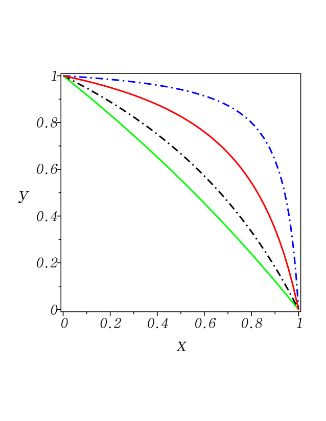
Figure 2:

Fig. 2: (Color online) Dimensionless virtual temperature $y=T_{v}/T_{2}$ in (1) versus dimensionless quantity $x=\alpha$. From the bottom, “low-temperature” regime: (I) (solid, green): $T_{1}=5$ and $T_{2}=1$, (II) (dashdot, black): $T_{1}=2$ and $T_{2}=1$; “high-temperature” regime: (III) (solid, red): $T_{1}=19$ and $T_{2}=15$, (IV) (dashdot, blue): $T_{1}=16$ and $T_{2}=15$.

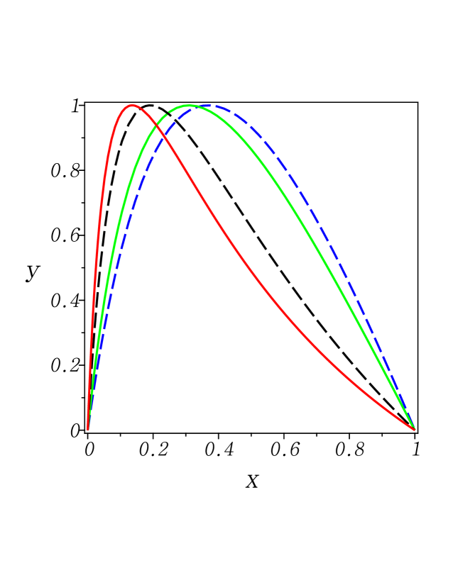
Figure 3:

Fig. 3: (Color online) Normalized specific cooling load $y={\mathcal{L}}_{3}/{\mathcal{L}}_{m}$ (as a “measure of irreversibility”) given in (13) versus normalized efficiency $x=\eta_{\mbox{\scriptsize fr}}/\eta_{\mbox{\tiny C}}$. Let $t_{1}:=T_{1}/T_{2}$ and $t_{3}:=T_{3}/T_{2}$. From the left in maximum value position $x_{m}$, (I) (solid, red): $t_{1}=3$ and $t_{3}=0.8$; (II) (dash, black): $t_{1}=2$ and $t_{3}=0.8$; (III) (solid, green): $t_{1}=3$ and $t_{3}=0.3$; (IV) (dash, blue): $t_{1}=2$ and $t_{3}=0.3$.

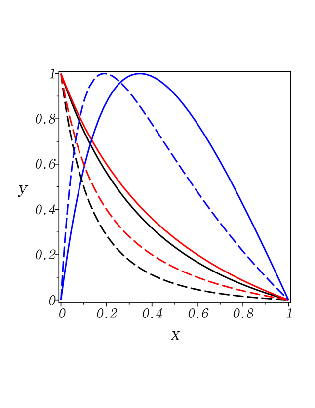
Figure 4:

Fig. 4: (Color online) Normalized heat flux $y=\dot{q}_{j}:=\dot{Q}_{j}/(\dot{Q}_{j})_{m}$ in (17) versus normalized efficiency $x=\eta_{\mbox{\scriptsize fr}}/\eta_{\mbox{\tiny C}}$, where $j=1,2,3$, and $(\dot{Q}_{j})_{m}$ denotes maximum value of $\dot{Q}_{j}$. Let $t_{1}:=T_{1}/T_{2}$ and $t_{3}:=T_{3}/T_{2}$. Dashed curves represent the case of $(t_{1},t_{3})=(2,0.8)$: From the bottom at $x=1/2$, (I) $\dot{q}_{1}$ (black); (II) $\dot{q}_{2}$ (red); (III) $\dot{q}_{3}$ (blue) being the cooling flux. Solid curves represent the case of $(t_{1},t_{3})=(2,0.4)$ and follow along the same lines.

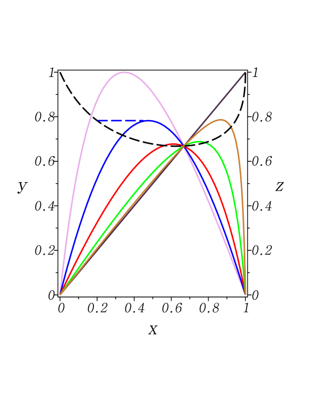
Figure 5:

Fig. 5: (Color online) Solid lines: Dimensionless thermoeconomic criterion $y={\mathcal{F}}_{c}=\{a^{\prime}\,x^{-1}+b^{\prime}\,({\mathcal{L}}_{3}/{\mathcal{L}}_{m})^{-1}\}^{-1}$ in (18) versus normalized efficiency $x=\eta_{\mbox{\scriptsize fr}}/\eta_{\mbox{\tiny C}}$, where $a^{\prime}=a/\eta_{\mbox{\tiny C}}$ and $b^{\prime}=b/{\mathcal{L}}_{m}$. We set $b^{\prime}=1-a^{\prime}$, and $(t_{1},t_{3})=(2,0.4)$. From the bottom at $x=0.9$: (I) $a^{\prime}=0$ (plum) representing ${\mathcal{L}}_{3}/{\mathcal{L}}_{m}$; (II) $a^{\prime}=0.2$ (blue); (III) $a^{\prime}=0.5$ (red); (IV) $a^{\prime}=0.8$ (green); (V) $a^{\prime}=0.95$ (gold); (VI) $a^{\prime}=1$ (violet) being a straight line $y=x$. In comparison, a dashed (black) curve $z={\mathcal{F}}_{m}(a^{\prime})$ versus $x=a^{\prime}$ is also put, which shows the maximum value of $y$ for a given $a^{\prime}$; e.g., in case of $a^{\prime}=0.2$, the curve $y$ (blue) has its maximum value of $0.78262={\mathcal{F}}_{m}(0.2)$, as indicated by the segment of dash line (blue).

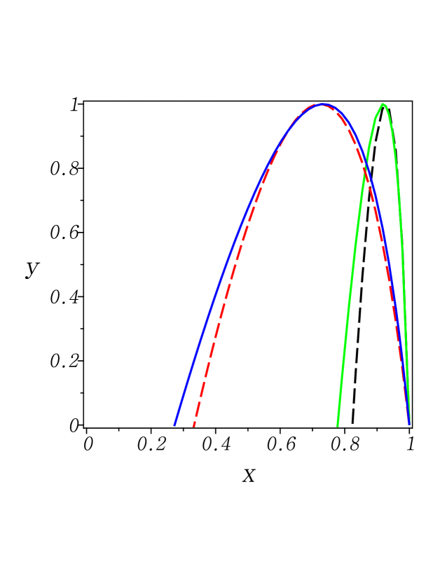
Figure 6:

Fig. 6: (Color online) Normalized specific cooling load $y={\mathcal{L}}_{3}/{\mathcal{L}}_{m}$ in (20) versus $x=\alpha$. From the right in position of $x=\alpha_{\mbox{\tiny C}}\,(\neq 1)$ at which $y=0$: (I) (dash, black): $t_{1}=2$ and $t_{3}=0.3$, (II) (solid, green): $t_{1}=3$ and $t_{3}=0.3$, (III) (dash, red): $t_{1}=2$ and $t_{3}=0.8$, (IV) (solid, blue): $t_{1}=3$ and $t_{3}=0.8$.

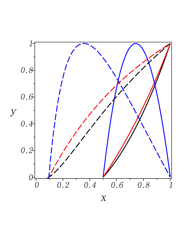
Figure 7:

Fig. 7: (Color online) Normalized heat flux $y=\dot{q}_{j}:=\dot{Q}_{j}/(\dot{Q}_{j})_{m}$ (to be derived from (20)) versus $x=\alpha$, where $j=1,2,3$, and $(\dot{Q}_{j})_{m}$ denotes maximum value of $\dot{Q}_{j}$. Solid curves represent the case of $(t_{1},t_{3})=(2,2/3)$ equivalent to $\alpha_{\mbox{\tiny C}}=1/2$: From the bottom at $x=0.6$, (I) $\dot{q}_{1}$ (black); (II) $\dot{q}_{2}$ (red); (III) $\dot{q}_{3}$ (blue). Dashed curves represent the case of $(t_{1},t_{3})=(2,0.95)$ and follow similarly.

References

- (1) Intergovernmental Panel on Climate Change 2007, in the 4th Assessment Report of the Intergovernmental Panel on Climate Change (Geneva, 2007).
- (2) Han J.-C., Dutta S., and Ekkad S., Gas Turbine Heat Transfer and Cooling Technology (2nd ed., CRC Press, 2012).
- (3) Andresen B., Finite-time thermodynamics (University of Copenhagen, 1983).
- (4) Sieniutycz S. and Salamon P., Finite-Time Thermodynamics (Taylor Francis, New York, 1990).
- (5) Sieniutycz S. and Shiner J. S., J. Non-Equil. Thermodyn. 19, 303 (1994).
- (6) Wu C., Energy Convers. Mgmt 37, 1509 (1996).
- (7) Berry R. S., Kazakov V. A., Sieniutycz S., Szwast Z., and Tsirlin A. M., Thermodynamic Optimization of Finite-Time Processes (Wiley, Chichester, 1999).
- (8) Sahin B. and Kodal A., Energy Convers. Mgmt 40, 951 (1999).
- (9) Kodal A., Sahin B., Ekmekci I., and Yilmaz T., Energy Convers. Mgmt 44, 109 (2003).
- (10) Qin X., Chen L., Sun F., and Wu C., Applied Energy 81, 420 (2005).
- (11) Gemmer J., Michel M., and Mahler G., Quantum Thermodynamics (Springer, Berlin, 2004).
- (12) Linden N., Popescu S., and Skrzypczyk P., Phys. Rev. Lett. 105, 130401 (2010).
- (13) Popescu S., arXiv:1009.2536 (2010).
- (14) Skrzypczyk P., Brunner N., Linden N., and Popescu S., J. Phys. A 44, 492002 (2011).
- (15) Brunner N., Linden N., Popescu S., and Skrzypczyk P., Phys. Rev. E 85, 051117 (2012).
- (16) Chen Y.-X. and Li S.-W., Europhys. Lett. 97, 40003 (2012).
- (17) Matson J., A Bit Cold: Physicists Devise a Quantum Particle “Refrigerator”, Scientific American, September (2010).