Quantum-Bath Decoherence of Hybrid Electron-Nuclear Spin Qubits

thesis_date28082015 monthyear[]

Declaration

I, , confirm that the work presented in this thesis is my own. Where information has been derived from other sources, I confirm that this has been indicated in the thesis. The work contains nothing which is the outcome of work done in collaboration except where specifically indicated in the text.

Parts of this thesis have been published, or submitted for publication, as follows.

• Chapters 3 & 5: G. W. Morley, P. Lueders, M. Hamed Mohammady, S.J.B., G. Aeppli, C. W. M. Kay, W. M. Witzel, G. Jeschke, and T. S. Monteiro, Nature Materials 12, 103 (2013).

• Chapters 4 & 5: S.J.B., M. B. A. Kunze, M. H. Mohammady, G. W. Morley, W. M. Witzel, C. W. M. Kay, and T. S. Monteiro, Physical Review B 86, 104428 (2012).

• Chapters 5 & 6: S.J.B., G. Wolfowicz, J. J. L. Morton, and T. S. Monteiro, Physical Review B 89, 045403 (2014).

• Chapters 5 & 7: S.J.B., R.-B. Liu, and T. S. Monteiro, Physical Review B 91, 245416 (2015).

• Chapter 8: R. Guichard, S.J.B., G. Wolfowicz, P. A. Mortemousque, and T. S. Monteiro, Physical Review B 91, 214303 (2015).

thesis_date

Abstract

A major problem facing the realisation of scalable solid-state quantum computing is that of overcoming decoherence – the process whereby phase information encoded in a quantum bit (‘qubit’) is lost as the qubit interacts with its environment. Due to the vast number of environmental degrees of freedom, it is challenging to accurately calculate decoherence times $T_{2}$, especially when the qubit and environment are highly correlated.

Hybrid or mixed electron-nuclear spin qubits, such as donors in silicon, are amenable to fast quantum control with pulsed magnetic resonance. They also possess ‘optimal working points’ (OWPs) which are sweet-spots for reduced decoherence in magnetic fields. Analysis of sharp variations of $T_{2}$ near OWPs was previously based on insensitivity to classical noise, even though hybrid qubits are situated in highly correlated quantum environments, such as the nuclear spin bath environment of ²⁹Si impurities. This presented limited understanding of the underlying decoherence mechanism and gave unreliable predictions for $T_{2}$.

In this thesis, I present quantum many-body calculations of the qubit-bath dynamics, which (i) yield $T_{2}$ for hybrid qubits in excellent agreement with experiments in multiple regimes, (ii) elucidate the many-body nature of the nuclear spin bath and (iii) expose significant differences between quantum-bath and classical-field decoherence. To achieve these results, the cluster correlation expansion was adapted to include electron-nuclear state mixing. In addition, an analysis supported by experiment was carried out to characterise the nuclear spin bath for a bismuth donor as the hybrid qubit, a simple analytical formula for $T_{2}$ was derived with predictions in agreement with experiment, and the established method of dynamical decoupling was combined with operating near OWPs in order to maximise $T_{2}$. Finally, the decoherence of a ²⁹Si spin in proximity to the hybrid qubit was studied, in order to establish the feasibility for its use as a quantum register.

In memory of Siroun & Alidz

Nomenclature

• $J_{1}-J_{2}$.

• Donor electron ionization energy.

• Electronic spin gyromagnetic ratio.

• Nuclear spin gyromagnetic ratio.

• Nuclear spin operator, $\hat{\bf I}=(\hat{I}^{x},\hat{I}^{y},\hat{I}^{z})$.

• Electron spin operator, $\hat{\bf S}=(\hat{S}^{x},\hat{S}^{y},\hat{S}^{z})$.

• Vector of Pauli operators, $\hat{\bm{\sigma}}=(\hat{\sigma}^{x},\hat{\sigma}^{y},\hat{\sigma}^{z})$.

• $\hat{\sigma}^{x}\pm i\hat{\sigma}^{y}$, and similarly for $\hat{S}^{\pm}$ and $\hat{I}^{\pm}$.

• Bath spin Hamiltonian.

• Central spin system or qubit spin Hamiltonian.

• Interaction spin Hamiltonian.

• Total spin Hamiltonian, $\hat{H}_{\text{tot}}=\hat{H}_{\text{CS}}+\hat{H}_{\text{int}}+\hat{H}_{\text{bath}}$.

• Pseudospin Hamiltonian for central level $\left|{i}\right\rangle$.

• $e^{i\hat{h}_{i}t}$, for pseudospin Hamiltonian $\hat{h}_{i}$.

• $e^{i\hat{H}t}$, for Hamiltonian $\hat{H}$.

• Planck constant divided by $2\pi$.

• Spin-down.

• Initial bath state.

• Bath state correlated with central system state $\left|{i}\right\rangle$.

• Adiabatic eigenstate of mixed electron-nuclear spin system (hybrid qubit implementation).

• Spin-up.

• Eigenstates of central spin system labelled in order of increasing energy.

• Lower central system level.

• Magnetic resonance transition from an upper ($\left|{u}\right\rangle$) to a lower ($\left|{l}\right\rangle$) level in energy.

• Upper central system level.

• Dipolar tensor.

• Hyperfine tensor.

• Coherence as a function of time $t$.

• Permeability of free space.

• Far from OWPs.

• $\omega^{\pm}=\omega_{u}\pm\omega_{l}$.

• Electron spin Larmor frequency, $\omega_{0}=\gamma_{e}B$.

• Pseudospin frequency.

• Dipolar prefactor of $T_{2}$ formula, with crystal orientation angle $\theta$.

• Refocusing pulse as used in the Hahn spin echo sequence for example.

• Pulse to create a qubit superposition.

• Dynamical decoupling pulse spacing in time.

• $\theta^{\pm}=\theta_{u}\pm\theta_{l}$.

• Pseudofield angle from $z$-axis of Bloch sphere.

• Cubic lattice parameter.

• Strength of hyperfine interaction between the donor electron spin and host nuclear spin of Si:$X$.

• Zeeman magnetic field strength.

• Secular dipolar interaction strength.

• Transition frequency-magnetic field gradient.

• Nuclear spin quantum number.

• Silicon donor (Si:$X$) host nuclear spin quantum number.

• Strength of hyperfine interaction between an electron spin and a bath nuclear spin.

• Fermi contact strength.

• Boltzmann constant.

• Nuclear spin magnetic quantum number.

• Electronic spin magnetic quantum number.

• Number of dynamical decoupling pulses.

• Non-trivial qubit-bath dynamics arising from $n$ bath spins and involving entanglement between the qubit and bath.

• Polarisation for level $\left|{i}\right\rangle$, $P_{i}=\left\langle{i}\right|\hat{S}^{z}\left|{i}\right\rangle$.

• Electron spin quantum number ($S=\tfrac{1}{2}$).

• 4 GHz ESR excitation frequency.

• Temperature.

• Relaxation time.

• Coherence time.

• Coherence time sometimes used to distinguish donor-donor decoherence from nuclear spin diffusion decoherence characterized by $T_{2}$.

• Ensemble FID coherence time.

• 9.7 GHz ESR excitation frequency.

• Points on a continuous spherical surface which have a one-to-one correspondence with quantum states of a qubit.

• Cluster correlation expansion.

• CCE truncated at, or calculated up to, $k$-th order.

• In general, a multi-spin system resonant with control pulses and distinguished from bath or environmental spins.

• $\tfrac{1}{\sqrt{2}}\left(\left|{u}\right\rangle+\left|{l}\right\rangle\right)$

• Carr-Purcell-Meiboom-Gill dynamical decoupling pulse sequence.

• Temperature $T\lesssim 15$ K.

• Clock transition ($df/dB=0$).

• Crystal structure of silicon or diamond.

• Flip-flops between central spin system and bath spins.

• Electron-nuclear double resonance.

• Silicon with reduced ²⁹Si spin impurities.

• Equivalent pairs.

• Electron spin resonance.

• Magnetic resonance transition ESR-forbidden at high fields (i.e., a pure NMR transition at high fields.)

• $\left|{\pm,m}\right\rangle\leftrightarrow\left|{\mp,m-1}\right\rangle$ transitions.

• Free induction decay.

• Spin Hamiltonian terms of the form $\hat{S}_{1}^{-}\hat{S}_{2}^{+}+\hat{S}_{1}^{+}\hat{S}_{2}^{-}$.

• A region of strong detuning caused by an electronic spin or hybrid qubit where nuclear flip-flops are suppressed.

• Full width at half maximum.

• Multi-spin system with eigenstates which mix the Zeeman basis.

• Magnetic field region of hybrid qubit where there is strong mixing of the Zeeman basis.

• Flip-flops between bath spins coupled to a central spin system.

• Decoherence caused by flipping bath spins as well as the central spin system with the application of $\pi$-pulses.

• Spin Hamiltonian terms involving products of only $z$-projection operators.

• Landau-Zener.

• Silicon with 4.67% ²⁹Si spin impurities.

• Nuclear magnetic resonance.

• $\left|{\pm,m}\right\rangle\leftrightarrow\left|{\pm,m-1}\right\rangle$ transitions.

• Spin Hamiltonian terms not involving products of $z$-projection operators, and often involving flip-flop terms.

• Spin diffusion of an electronic spin or hybrid qubit in a nuclear spin bath.

• Nitrogen vacancy.

• Optimal working point ($P_{u}=P_{l}$).

• $2$-body correlations.

• Nuclear spins nearby an electronic spin or hybrid qubit in the frozen core region.

• Pseudospin precession axis.

• Two-level system described by the space spanned by the non-polarized eigenstates of a two-spin-1/2 system ($\{\left|{\downarrow\uparrow}\right\rangle,\left|{\uparrow\downarrow}\right\rangle\}$).

• Decoherence involving no central state depolarisation.

• Environment with strong system-environment back-action (involving entanglement). A spin bath is an example.

• Quantum bit or two-level system.

• Ruderman-Kittel-Kasuya-Yosida or hyperfine-mediated interaction.

• $X$-doped silicon.

• Environment surrounding a central spin system and made up of spin species.

• Any indirect flip-flop-type decoherence mechanism.

• C++ spin decoherence library written by S.J.B..

• Part of the total detuning on bath flip-flop dynamics which is important for driving decoherence.

• Part of the total detuning on bath flip-flop dynamics which always suppresses decoherence.

• Magnetic field region of hybrid qubit where there is no longer strong mixing of the Zeeman basis.

• Basis of product eigenstates of a sum of uncoupled Zeeman (high magnetic field) spin Hamiltonians.

1  |  Introduction

Decoherence is the loss of phase information encoded in a quantum system as the system interacts with a far larger environment (Zurek, 2003). A certain degree of immunity from the destructive effects of decoherence, sometimes even achievable by directly suppressing the process, is an essential requirement for the successful realisation of technological devices that actively exploit quantum phenomena. These include fault-tolerant quantum processors (Shor, 1996) and quantum memory (Simon et al., 2010). Thus, it is of great practical importance to accurately predict the timescale of decoherence – characterised by the coherence time $T_{2}$ – and also to develop methods of extending $T_{2}$ times.

It is also of fundamental interest to understand how decoherence due to quantum environments differs from decoherence driven by classical noise sources. By quantum environment, we mean that the system encoding the quantum information is situated in an environment with which it is highly correlated or entangled, leading to significant system-environment ‘back-action’ and environment-memory effects (Breuer and Petruccione, 2002; Maniscalco and Petruccione, 2006; Mazzola et al., 2012). More specifically, the environment dynamics is sensitive to the state of the central spin system (Yao et al., 2006; Liu et al., 2007). A quantum spin bath is an example of such an environment; in general, decoherence of a central spin system coupled to a spin bath arises from many-body spin interactions inside the bath (Witzel et al., 2005; Yang and Liu, 2008a). The extent to which many-body correlations play a role in quantum dynamics is of broad interest in condensed matter physics (Ma et al., 2014).

Thus, in this thesis, we address problems of both practical and fundamental physical importance. On one hand, understanding and reliably predicting decoherence provides a useful guide to experimentalists working on implementing quantum technologies; also of importance is developing methods of mitigating decoherence. On the other hand, the study of decoherence serves as a valuable tool to probe the rich physics of many-body quantum systems and the extent to which these can be approximated using classical models.

1.1 Motivation

Individual electronic and nuclear spins in silicon are among the prime contenders for realising scalable quantum technologies (Zwanenburg et al., 2013). In particular, due to its long-lived coherence and fast manipulation time, the electronic spin of a shallow donor in silicon is a promising candidate for implementing the quantum analogue of the classical bit – the qubit; in a solid state system (Morley, 2015).

Decoherence for silicon donor qubits is often limited by the naturally-occurring ²⁹Si nuclear spin bath (de Sousa and Das Sarma, 2003a, b). The phosphorus donor has been widely studied (Kane, 1998), but more recently, there has been growing interest in bismuth, the deepest of the Group V donors in silicon (Morley et al., 2010; George et al., 2010; Mohammady et al., 2010). It was proposed that decoherence would be strongly suppressed and $T_{2}$ significantly enhanced for the bismuth system at particular magnetic field values termed ‘optimal working points’ (OWPs) (Mohammady et al., 2010). The presence of OWPs at experimentally accessible magnetic fields is due to the strong quantum state-mixing of the donor electronic spin with the host nuclear spin, hence the term ‘hybrid electron-nuclear qubit’.

The scenario of decoherence driven by a spin bath is not only limited to silicon donor qubits (de Sousa and Das Sarma, 2003b; Witzel et al., 2005; Abe et al., 2010; Witzel et al., 2010), but is of considerable significance for a range of other physical implementations of quantum information processing, including quantum dots in environments with a variety of nuclear spin impurities (de Sousa and Das Sarma, 2003b; Witzel et al., 2005; Yao et al., 2006; Liu et al., 2007; Witzel and Das Sarma, 2008; Weiss et al., 2012, 2013; Webster et al., 2014), and nitrogen-vacancy (NV) centres in the ¹³C spin bath of diamond.

At first glance, it seems impossible to accurately solve for the closed system-bath dynamics for a bath of spins, due to the large number of spin degrees of freedom involved. Nevertheless, cluster expansion techniques, the most general of which is the cluster correlation expansion (CCE) (Yang and Liu, 2008a, b, 2009) have provided a solution. In the CCE and analogous formalisms, accurate simulation of experimental coherence decays becomes computationally tractable since the bath is decomposed into independent contributions from many small sets or clusters of spins (de Sousa and Das Sarma, 2003a, b; Witzel et al., 2005; Witzel and Das Sarma, 2006; Yao et al., 2006). Fortunately, it turns out that for most problems of practical interest in quantum information the expansions converge for clusters containing at most half a dozen or so spins.

The CCE has been used with considerable success to model central spin decoherence in a variety of systems, including the the silicon spin bath, despite the large number of bath spins involved (Abe et al., 2004; Witzel and Das Sarma, 2006; Abe et al., 2010; Witzel et al., 2010). However, in all cases prior to the work presented herein, the CCE was implemented and applied for the central system limited to the case of a simple electronic or nuclear spin. Moreover, previous calculations of $T_{2}$ for the hybrid qubit relied on analyses involving classical noise models (George et al., 2010). As we shall see, these models do not give reliable $T_{2}$ times in all regimes. In George et al. (2010), weak state-mixing of the central spin in a nuclear spin bath was investigated by simply allowing for the variation of an effective electronic gyromagnetic ratio which quantifies the response to external classical magnetic fields. Although this classical treatment and analogous ones are valid in some regimes, they do not reliably describe the crucial OWP regions, and also, cannot account for certain ‘forbidden transitions’ which allow fast quantum control of the hybrid qubits. Our primary aim was to solve this problem by considering the full quantum state-mixing of the hybrid qubit in many-body calculations of decoherence driven by a nuclear spin bath.

It is also of experimental interest to investigate how and when the commonly applied method of dynamical decoupling (Viola and Lloyd, 1998) can be combined with operating near OWPs in order to further extend coherence times. In dynamical decoupling, the central qubit is subjected to a sequence of electromagnetic pulses separated in time; environmental noise is suppressed when the frequency of the noise spectrum is less than or equal to the inverse of the pulse spacing in the sequence.

However, interest in the silicon spin bath has recently shifted beyond its destructive decohering role. For example, the need remains to establish the feasibility of using nuclear spin impurities for quantum information applications (Cappellaro et al., 2009; Akhtar et al., 2012; Pla et al., 2014), especially when the nuclear spins are in proximity to a donor. For example, nuclear spins in the bath can act as registers storing quantum information (Cappellaro et al., 2009; Waldherr et al., 2014; Taminiau et al., 2014).

As mentioned in the opening paragraphs, understanding decoherence is not only motivated by practical reasons. It is of fundamental importance in physics to determine the differences between decoherence caused by classical magnetic field fluctuations and decoherence driven by quantum baths. Also, it is interesting to elucidate the many-body nature of a spin bath (Witzel et al., 2005; Yang and Liu, 2008a; Witzel et al., 2010; Zhao et al., 2012a; Witzel et al., 2012; Ma et al., 2014); are experiments fully described by only considering sets of independent pairs of bath spins? Or are sets containing $n>2$ bath spins required? In other words, we wish to determine to what degree many-body system-bath correlations are important.

In many cases of central spin decoherence problems, the dominant contribution to the combined dynamics arises from pairs of bath spins (the so-called pair correlation) (Yao et al., 2006); in effect, from the magnetic noise due to the independent ‘flip-flopping’ of spin pairs. Contributions from larger clusters are usually only needed for high accuracy (Witzel et al., 2010, 2012; Zhao et al., 2012a).

1.2 Outcomes

In the work presented herein, the numerical CCE method was adapted and implemented to include the state-mixing of the hybrid qubit (details of the code are given in Appendix A). In fact, any complex multi-spin system coupled to other spin systems in the interacting many-body bath can be simulated with our implementation. It provided the first theoretical demonstration of suppression of spin bath decoherence near OWPs (Balian et al., 2012), subsequently verified in experiments (Wolfowicz et al., 2013; Balian et al., 2014). Coherence decays and $T_{2}$ times were obtained in perfect agreement with experiments for forbidden transitions (Morley et al., 2013), near OWPs (Balian et al., 2014), and in the usual regimes far from OWPs (Balian et al., 2014). As for dynamical decoupling, in order to extend the already long coherence times near OWPs, a large number of dynamical decoupling pulses must be applied, in contrast to the usual regimes away from OWPs (Balian et al., 2015).

As a parallel study to complement our understanding of nuclear spin bath decoherence, we analysed the system-bath interaction for the case of the hybrid qubit, and found clear spectroscopic signatures of the central state-mixing and of OWPs by comparing our theory with pulsed magnetic resonance experiments (Balian et al., 2012). These experiments resolved groups of nuclear bath spins at equivalent crystal sites and thus motivated us to investigate the feasibility of using nuclear spins for quantum memory. We studied the decoherence of such nuclear impurities in proximity to a donor and found that the nuclear $T_{2}$ time far exceeds that for the case of an impurity in the absence of a donor (Guichard et al., 2015).

It was already mentioned that some effects of the state-mixing of the hybrid qubit can be adequately described using classical noise models. In some cases, this description is sufficient, however, we find that near the important OWP regions, a full quantum treatment of the system-bath dynamics including the central system mixing is necessary for obtaining the experimentally observed coherence decays (Balian et al., 2014).

We also identify qualitative differences between the classical and quantum models, using a closed-form analytical $T_{2}$ formula for the decoherence of donors in silicon which we derive (Balian et al., 2014). The formula also predicts $T_{2}$ values in excellent agreement with experiment and numerical CCE calculations. Also, we find that classical noise models sometimes give ‘false positives’ for the existence of sweet-spots for decoherence in quantum baths.

Finally, we present the only case where there is almost complete suppression of the usual pair correlations provided that one is operating near OWPs and with sufficiently low orders of dynamical decoupling (Balian et al., 2015). We find that clusters containing at least three bath spins (3-body clusters) are required to recover the experimentally measured decays.

For the rest of this chapter, before providing an outline of the thesis, we review the field of quantum information processing with donor qubits in silicon, the various methods of mitigating decoherence, and the quantum theory of spin decoherence. We start with briefly defining the general problem of decoherence and give a more comprehensive account for the case of spin baths in Chapter 2.

1.3 The Problem of Decoherence

All known quantum algorithms offering speed-up over their classical counterparts rely either on quantum superposition, quantum entanglement or both (Nielsen and Chuang, 2010). We begin by introducing these two concepts. In quantum computing, the classical two level system known as the ‘bit’ is replaced by its quantum version – the qubit (Audretsch, 2007; Nielsen and Chuang, 2010):

$$\left|{\psi}\right\rangle=\alpha\left|{0}\right\rangle+\beta\left|{1}\right\rangle.$$ (1.1)

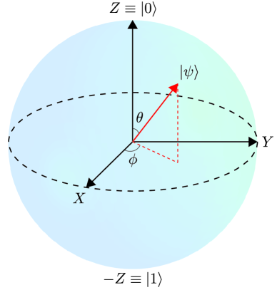
Figure 1.1: The states of any two-level quantum system (a qubit) can be represented as points on the surface of the Bloch sphere (Nielsen and Chuang, 2010).

The classical bit is always either in state $\left|{0}\right\rangle$ or $\left|{1}\right\rangle$, whereas the qubit can be in any general superposition $\left|{\psi}\right\rangle$ of the two states forming the complete orthonormal basis $\{\left|{0}\right\rangle,\left|{1}\right\rangle\}$, as shown in Equation (1.1), where $\alpha$ and $\beta$ are complex numbers. As illustrated in Figure 1.1, all normalised single qubit states ($|\alpha|^{2}+|\beta|^{2}=1$) can be represented as points on the surface of a unit sphere known as the Bloch sphere, with the polar ($\theta$) and azimuthal ($\phi$) angles related to the amplitudes $\alpha$ and $\beta$ according to

$$\alpha =\cos{\left(\frac{\theta}{2}\right)}, \beta=e^{i\phi}\sin{\left(\frac{\theta}{2}\right)}.$$ (1.2)

Quantum entanglement is a property of multipartite quantum systems. Two qubits ($A$ and $B$) are said to be entangled if their combined state is not separable, or equivalently, not a product state such as $\left|{0}\right\rangle_{A}\otimes\left|{1}\right\rangle_{B}$. For example,

$$\left|{\psi}\right\rangle_{AB}=\frac{1}{\sqrt{2}}\left(\left|{0}\right\rangle_{A}\otimes\left|{1}\right\rangle_{B}+\left|{1}\right\rangle_{A}\otimes\left|{0}\right\rangle_{B}\right)$$ (1.3)

is a (maximally) entangled state and has no classical analogue.

The loss of information contained in a qubit state due to its interaction with a far larger environment is quantified by two characteristic timescales: $T_{1}$ and $T_{2}$ (Schweiger and Jeschke, 2001). These are illustrated in Figure 1.2. Decoherence is the mechanism by which the quantum phase information is lost and is represented by $T_{2}$ (Breuer and Petruccione, 2002). The single qubit state can be expressed using a density matrix which acts on the 2-dimensional Hilbert space (spanned by the basis $\{\left|{0}\right\rangle,\left|{1}\right\rangle\}$):

$$\bm{\rho}=\left(\begin{array}[]{cc}|\alpha|^{2}&\alpha\beta^{*}\\ \alpha^{*}\beta&|\beta|^{2}\end{array}\right).$$ (1.4)

The phase information is contained in the off-diagonals of the density matrix and as the system evolves in its environment, the decay rate of the off-diagonals is given by $1/T_{2}$.

Figure 1.2: Loss of information encoded in a qubit can be (a) a classical or (b) a purely quantum process. (a) Classical loss of information is decay along the $z$-axis of the Bloch sphere (Figure 1.1) and is characterised by $T_{1}$. (b) Decoherence is the process by which the phase information is lost (on a timescale defined by $T_{2}$) and can be visualized as ‘spreading’ of the qubit state on the equator of the Bloch sphere.

Classical information is lost by ‘$T_{1}$’ or ‘relaxation’ processes which involve direct bit flips (depolarisation); i.e. $\left|{0}\right\rangle\leftrightarrow\left|{1}\right\rangle$. Unlike a typical ‘$T_{2}$ process’, relaxation involves the exchange of some form of energy, usually mediated by phonons in the bath and is manifested as time decay in the diagonals of the density matrix. Relaxation is also a source of errors in quantum computing, however, for our systems of interest, temperatures are low enough ($<15$ K) to completely ignore $T_{1}$ processes, and the $T_{1}$ time far exceeds the coherence time $T_{2}$.

Given a qubit system prepared in some superposition, or two qubits in an entangled state, it is desirable to preserve these initial states for as long as possible as the system interacts with its often uncontrollable environment. Ignoring relaxation, this translates to extending the coherence time $T_{2}$. A wide range of quantum technologies, including fault-tolerant quantum computation, rely on coherence times longer than the times required to navigate the state on the Bloch sphere, and preferably as long as possible.

1.4 Quantum Information Processing in Silicon

There are two primary advantages of choosing the silicon platform for quantum information applications. First, silicon is a good ‘semiconductor vacuum’; in other words, coherence times in silicon are long compared to those in other solids. Second, there has been decades of unprecedented technological progress in conventional silicon electronics since the invention of the transistor around 1950; silicon is also cheap and easily available, and has good potential for scalability. In this section, we review the recent progress in silicon quantum electronics with a particular focus on the hybrid donor qubit. Zwanenburg et al. (2013) provide a recent and comprehensive review of the field.

A novel proposal for quantum computing in silicon was put forward by Kane (Kane, 1998), in which the nuclear spins of phosphorus donors would be used as qubits, with the donor electrons mediating qubit interactions. The nuclei were chosen as qubits since nuclear spin coherence times typically far exceed electronic spin coherence times. However, the price to pay is the much longer manipulation time of nuclear spins compared to that of electrons. More recently, coherence times of electronic spins have caught up and interest has shifted towards using electronic spins as long-lived qubits with fast quantum control.

In our case, the qubit is formed out of a pair of eigenstates of the mixed system comprised of a host nuclear spin interacting with the donor electron spin. Hence, it only makes strict sense to talk of separate electronic and nuclear spins of the mixed system in the high-field limit, where the interaction Hamiltonian becomes negligible. As we shall see, the advantages of the hybrid qubit for quantum computing arise when operating in regimes where the electronic and nuclear spin states are strongly mixed.

Most experiments measuring coherence times are performed on ensembles of spins. However, for quantum information applications it is essential to build to single-atom devices. Fortunately, in some cases, ensemble $T_{2}$ measurements are in good agreement with the corresponding $T_{2}$ for single-atom devices. It is important to note that there has been much progress in recent years in single-spin detection and read-out for both quantum dots (Kawakami et al., 2014; Veldhorst et al., 2014) and donor qubits in silicon (Morello et al., 2010; Pla et al., 2012, 2013; Muhonen et al., 2014; Pla et al., 2014).

1.4.1 Silicon Spin Bath

In natural silicon, 4.67% of crystal sites are occupied by the nuclear spin-1/2 ${}^{29}\text{Si}$ isotope, rather than the spin-0 ${}^{28}\text{Si}$. It is this spin bath that provides the leading source of decoherence in silicon at low temperatures ($T\lesssim 15$ K). For a donor electron spin (without OWP or dynamical decoupling enhancement), $T_{2}$ is limited to a few hundred microseconds (Tyryshkin et al., 2003; George et al., 2010; Morley et al., 2010). Similarly, a spin bath highly rich in nuclear spins exists for III-V semiconductor quantum dots, limiting $T_{2}$ to less than 1 $\mu$s (Koppens et al., 2008). This is also the case in diamond, where decoherence is instead driven by 1% ¹³C spin-1/2 isotopes, resulting in $T_{2}\simeq 200$ $\mu$s of an NV centre (Gaebel et al., 2006).

A successful means of controlling decoherence is to employ isotopically enriched samples, whereby the percentage of ²⁹Si impurities is reduced. The donor electron spin in such samples can exhibit long $T_{2}$ times up to 20 ms (Tyryshkin et al., 2012). However, isotopic enrichment is a difficult process and some nuclear spins remain. Even in isotopically enriched silicon, $T_{2}$ of an ensemble of donors is limited by an all-dipolar many-body spin system (Witzel et al., 2010; Tyryshkin et al., 2012; Wolfowicz et al., 2012; Witzel et al., 2012). Therefore, studying the nuclear bath is useful even in the case of its absence in enriched samples as the decoherence mechanisms in that case can be analogous to the case of the nuclear bath. Moreover, as discussed below, the nuclear impurity spins can be potentially useful for quantum memory (Akhtar et al., 2012; Pla et al., 2014; Guichard et al., 2015).

1.4.2 Donors in Silicon

A promising approach for silicon-based quantum information processing and memory involves electronic or nuclear spins of donor atoms in silicon, which are amenable to high fidelity manipulation by means of electron spin resonance (ESR) and nuclear magnetic resonance (NMR), respectively. Most studies have considered phosphorus (${}^{31}\text{P}$) donors in silicon. More recently, several different groups have investigated another Group V donor, ${}^{209}\text{Bi}$. The bismuth system offers new possibilities for quantum information processing. For example, strong optical hyperpolarisation was demonstrated (Morley et al., 2010; Sekiguchi et al., 2010), allowing for efficient initialization of the host nuclear spin. Transitions which are forbidden at high magnetic fields and which allow for fast control of the hybrid bismuth system were predicted (Mohammady et al., 2010, 2012) and observed later in Morley et al. (2013). Most importantly, the bismuth donor has OWPs, where both spin bath decoherence is suppressed (Balian et al., 2012; Wolfowicz et al., 2013; Balian et al., 2014) and the donor becomes insensitive to classical field fluctuations (e.g. instrument noise) (Mohammady et al., 2012; Wolfowicz et al., 2013). Near OWPs in natural silicon, the electronic spin coherence time is increased by over two orders of magnitude (Wolfowicz et al., 2013; Balian et al., 2014) from $0.5$ ms (Morley et al., 2010; George et al., 2010). A review of donors in silicon for quantum information processing was recently conducted by Morley (2015).

1.4.3 Nuclear Spin Impurities

Interest in nuclear spin impurities has now moved far beyond their role as a destructive source of decoherence. One application is sensing of a few nuclear ²⁹Si spins in silicon (Müller et al., 2014; Lang et al., 2015) and ¹³C spins in diamond (Zhao et al., 2011a; Kolkowitz et al., 2012; Zhao et al., 2012b; Kolkowitz et al., 2012; Taminiau et al., 2012; Müller et al., 2014). Another is using the nuclear spins for quantum memory (Ladd et al., 2005; Robledo et al., 2011; Akhtar et al., 2012; Pla et al., 2014; Guichard et al., 2015; Wolfowicz et al., 2015b). There is even a proposal for an all-silicon quantum computer using ²⁹Si spins (Ladd et al., 2002). The coherence time of a single ²⁹Si nuclear spin was measured at about 6 ms (Pla et al., 2014), in good agreement with measurements in ensembles (Dementyev et al., 2003).

Recently, quantum registers were demonstrated in diamond by combining the central electronic qubit with proximate nuclear spins (Cappellaro et al., 2009; Waldherr et al., 2014; Taminiau et al., 2014). The decoherence mechanisms of nuclear spins proximate to a donor in silicon was studied in Guichard et al. (2015), yielding coherence times in excellent agreement with the measured timecale of 1 s in Wolfowicz et al. (2015b).

1.5 Extending Coherence Lifetimes

There are two distinct techniques of proven effectiveness for extending the coherence lifetime of spin qubits without having to eliminate the nuclear spin impurities. One is dynamical decoupling, whereby the qubit is subjected to a carefully timed sequence of control pulses; the other is tuning the qubit towards OWPs, which are sweet-spots for reduced decoherence in magnetic fields. It is also of interest to combine the two techniques in order to achieve the longest coherence time.

1.5.1 Optimal Working Points

In 2002, a ground-breaking study of superconducting qubits established the usefulness of OWPs (Vion et al., 2002) which were then studied as parameter regimes where the system becomes – to first order – insensitive to fluctuations of external classical magnetic fields (Vion et al., 2002; Martinis et al., 2003; Makhlin et al., 2004; Makhlin and Shnirman, 2004; Falci et al., 2005; Ithier et al., 2005; Steger et al., 2011; Cywiński, 2014). More recently, OWPs were studied for coupled InGaAs quantum dots (Weiss et al., 2012, 2013) and in systems with substantial electron-nuclear spin mixing such as the bismuth donor system (Mohammady et al., 2010, 2012; Balian et al., 2012; Wolfowicz et al., 2013; Balian et al., 2014, 2015). OWPs for the bismuth donor were investigated theoretically in Mohammady et al. (2010, 2012); Balian et al. (2012, 2014) and Balian et al. (2015) and also experimentally (Wolfowicz et al., 2013; Balian et al., 2014), extending ensemble electronic spin $T_{2}$ times in natural silicon from $0.5$ ms (George et al., 2010; Morley et al., 2010) to $100$ ms (Wolfowicz et al., 2013). OWPs have also been investigated in isotopically enriched silicon (Wolfowicz et al., 2013). Measured electronic spin coherence times near and far from OWPs are summarized in in Table 1.1.

Sample	$T_{2}$ far from OWP (ms)	$T_{2}$ near OWP (ms)
Natural (with 29Si)	0.5	100
Enriched 28Si	20	2000

Table 1.1: Measured electronic spin coherence times $T_{2}$, illustrating the enhancement of coherence by operating near OWPs. The values shown are for the bismuth donor in silicon. In natural silicon and far from OWPs, coherence times were measured in George et al. (2010) and Morley et al. (2010). Away from OWPs in enriched samples, coherence times were measured in Wolfowicz et al. (2012) and Tyryshkin et al. (2012), and coherence times near OWPs were measured in Wolfowicz et al. (2013) and Balian et al. (2014).

It is useful to note that a wide variety of important defects in the solid state possess central spin state-mixing. These include donors in silicon (Morley, 2015), NV centres in diamond (Zhao et al., 2012a), transition metals in II-VI materials (George et al., 2013) and rare-earth dopants in silicates (Fraval et al., 2005; Wolfowicz et al., 2015a). The OWPs for spin bath decoherence of donors in silicon are a direct result of this mixing.

Earlier studies of other systems which have sweet-spots for insensitivity to classical field noise (Vion et al., 2002) led to theoretical analyses of the dependence of $T_{2}$ on field noise (Ithier et al., 2005; Martinis et al., 2003), both at and far from the sweet-spots. In contrast, it was only recently that a general analytical expression for $T_{2}$ (near and far from OWPs) was obtained for spin systems decohered by spin baths (Balian et al., 2014).

In Mohammady et al. (2010) and Mohammady et al. (2012), a set of minima and maxima were found in the transition frequency-field parameter space of dipole-allowed transitions of the bismuth donor. These $df/dB=0$ points, later dubbed ‘clock transitions’ (Wolfowicz et al., 2013), were first identified as OWPs: line narrowing and reduced sensitivity to temporal and spatial noise in magnetic field $B$ over a broad region of fields (closely related to $df/dB=0$ extrema) were found. They were also investigated experimentally (Wolfowicz et al., 2013). However, it was found later that the suppression of spin bath decoherence cannot be reliably explained in terms of the classical analysis involving $df/dB$ (Balian et al., 2012, 2014). In contrast, the insensitivity to classical field noise such as instrumental noise can in fact be adequately accounted for using $df/dB$ arguments (Mohammady et al., 2012; Wolfowicz et al., 2013).

The OWPs represent a potentially complementary technique, effective for both natural silicon and partially enriched samples. In addition, our work suggests that OWPs may also be effective in suppressing residual effects such as donor-donor interactions, which are the limiting decoherence mechanism in samples with low concentrations of nuclear impurities (Mohammady et al., 2010; Witzel et al., 2010; Wolfowicz et al., 2012; Witzel et al., 2012; Wolfowicz et al., 2013). Finally, we note that to date, all single-atom donor experiments have used phosphorus donors, and experiments measuring OWP coherence times have been for ensembles of bismuth donors.

1.5.2 Dynamical Decoupling

Dynamical decoupling is one of the most established methods for extending coherence times. It involves subjecting the qubit spin to a sequence of microwave or radio frequency pulses. A wide variety of solid state spin qubits have been studied under dynamical decoupling control; these include Group V donors in silicon, nitrogen vacancy centres in diamond (de Lange et al., 2010; Zhao et al., 2012a; Pham et al., 2012; Wang et al., 2012a; Bar-Gill et al., 2013), GaAs quantum dots (Zhang et al., 2008), rare-earth dopants in silicates (Fraval et al., 2005; Zhong et al., 2015), malonic acid crystals (Du et al., 2009) and adamantane (Peng et al., 2011).

The record coherence time for any spin system in a solid was measured at 6 hours in a rare-earth dopant using dynamical decoupling (Zhong et al., 2015). In silicon, the longest coherence time at room temperature exceeds 30 minutes with dynamical decoupling on ensembles of ionized donors in an isotopically enriched sample (Saeedi et al., 2013). At cryogenic temperatures, this coherence time is 3 hours. Coherence times enhanced by dynamical decoupling in ensemble donor experiments are summarized in Table 1.2 (enriched silicon) and Table 1.3 (natural silicon). For single donor devices, the extension of $T_{2}$ by dynamical decoupling for enriched and natural silicon are shown in Table 1.4 and Table 1.5 respectively. The coherence time of the ²⁹Si impurity has been extended to 25 s using dynamical decoupling (Ladd et al., 2005). As for a ²⁹Si spin in proximity to a donor, dynamical decoupling was recently applied to extend $T_{2}$ from 1 to 4 s (Wolfowicz et al., 2015b).

Coherence time $T_{2}$	Hahn spin echo (ms)	Dynamical decoupling (ms)
Electronic	20	500
Nuclear (neutral donor)	42,000	180,000
Nuclear (ionized donor)	27,000	10,800,000 (3 hours)

Table 1.2: Measured ensemble coherence times without (Hahn spin echo) and with dynamical decoupling in isotopically enriched ²⁸Si. Coherence times for the electron spin were measured in Tyryshkin et al. (2012), Wolfowicz et al. (2012) (Hahn), and Tyryshkin and Lyon (2012) (dynamical decoupling). Nuclear spin coherence times for the neutral and ionized donor were measured in Steger et al. (2012) and Saeedi et al. (2013) respectively.

Coherence time $T_{2}$	Hahn spin echo (ms)	Dynamical decoupling (ms)
Electronic	0.5	4
Nuclear (neutral donor)	1000	–

Table 1.3: Measured ensemble coherence times without (Hahn spin echo) and with dynamical decoupling in natural silicon. Nuclear spin coherence times were measured in Petersen et al. (2013), Balian et al. (2014) and Wolfowicz et al. (2015b). Electronic spin coherence times were measured in Tyryshkin et al. (2006), George et al. (2010), Morley et al. (2010) (Hahn), and Ma et al. (2014) (dynamical decoupling).

Coherence time $T_{2}$	Hahn spin echo (ms)	Dynamical decoupling (ms)
Electronic	1	550
Nuclear (neutral donor)	20	20
Nuclear (ionized donor)	1800	3560

Table 1.4: Measured single-donor device coherence times without (Hahn spin echo) and with dynamical decoupling in isotopically enriched ²⁸Si. The coherence times were measured in Muhonen et al. (2014). Note that for the neutral donor, the limiting decoherence mechanism was unknown, and is likely to not be of magnetic origin.

Coherence time $T_{2}$	Hahn spin echo (ms)	Dynamical decoupling (ms)
Electronic	0.2	0.5
Nuclear (neutral donor)	3.5	7
Nuclear (ionized donor)	60	132

Table 1.5: Measured single-donor device coherence times without (Hahn spin echo) and with dynamical decoupling in natural silicon. The electronic spin coherence times were measured in Pla et al. (2012) and the nuclear ones in Pla et al. (2013). The 7 ms value was obtained by private communication with the lead author of Pla et al. (2013).

It is also of practical importance to understand whether dynamical decoupling and OWP techniques may be advantageously combined for a quantum bath of nuclear spins. In Cywiński (2014), the two techniques were investigated for insensitivity to classical field noise. For donor electronic qubits in silicon, it is known that due to inhomogeneous broadening from naturally-occurring ²⁹Si spin isotopes, there was a significant gap between the $T_{2}\sim 100$ ms in natural silicon near an OWP (Wolfowicz et al., 2013; Balian et al., 2014), and the $T_{2}\sim 2$ s in isotopically enriched ²⁸Si with a low donor concentration at the same OWP (Wolfowicz et al., 2013). Also, dynamical decoupling may be useful when it is convenient to operate with the magnetic field close to but not exactly at the OWP. Recently, dynamical decoupling was used to extend $T_{2}$ near OWPs from $100$ ms to about 1 s (Balian et al., 2015; Ma et al., 2015).

1.5.3 Summary of Coherence Times

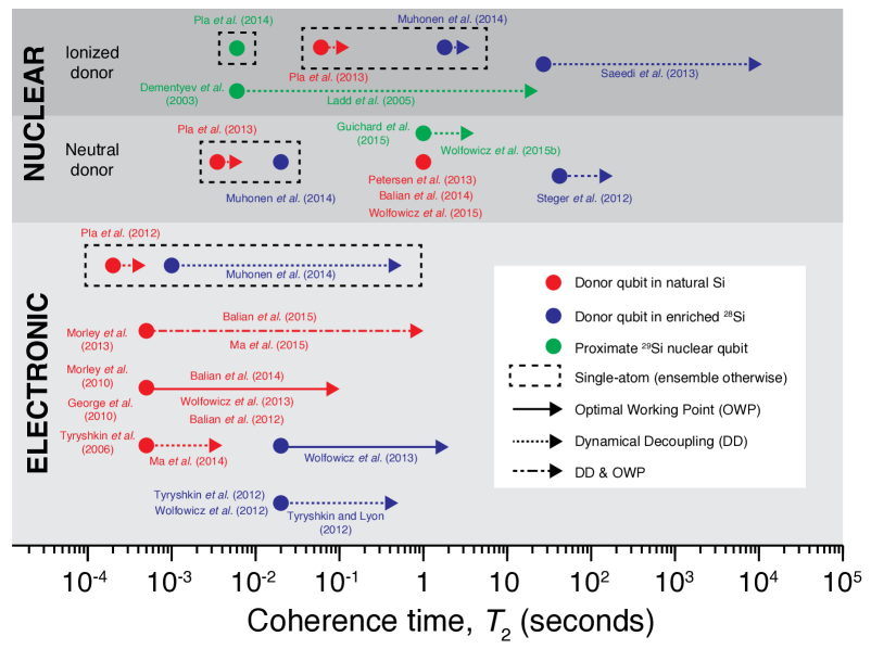
Figure 1.3: Cryogenic ($T\lesssim 15$ K) coherence times $T_{2}$ of donor qubits in natural or isotopically enriched silicon, extended by dynamical decoupling, optimal working points or by combining the two methods. Initial (unenhanced) times are for the Hahn spin echo. Electronic and nuclear spin coherence times correspond to microwave and radio frequency transitions respectively. Both single-atom and ensemble measurements are shown. Coherence times of proximate nuclear qubits are also shown for comparison.

Coherence times for hybrid donor qubits as well as proximate nuclear qubits in silicon are summarized in Figure 1.3. It is clear that the best method of enhancing coherence is by combining dynamical decoupling with operation at OWPs. It can also be seen that ensemble measurements of electronic spin coherence times are in good agreement with measurements in bulk. Nuclear coherence times are expected to exceed those for the electron due to the smaller gyromagnetic ratio of nuclei. Finally, by operating near OWPs in natural silicon (even without dynamical decoupling), coherence times can reach timescales measured in isotopically enriched silicon. We note that dynamical decoupling and operation near OWPs have not yet been investigated in enriched silicon.

1.6 Quantum Theories of Spin Decoherence

It goes without saying that solving for the joint system-bath dynamics as a closed system is a practically impossible task due to the large number of bath spins involved and the exponential complexity of numerical diagonalisation of the Hamiltonian. The framework of open quantum systems (Breuer and Petruccione, 2002) offers good approximations in many systems; however, treating cases with strong system-back action and environment-memory remains extremely challenging within this framework. Another inconvenience is that the usual form of Wick’s theorem is not available for spin degrees of freedom, thus preventing the use of Feynman diagrams in many-body spin dynamics (Witzel and Das Sarma, 2006).

For a long time, theories of spin decoherence were based on stochastic models which were phenomenological in that the noise spectrum of the environment had to be chosen. See, for example, Klauder and Anderson (1962). The ‘cluster expansion’ was the first “no-free-parameter” quantum theory of spin decoherence and was developed much later in 2006 (Witzel et al., 2005; Witzel and Das Sarma, 2006), following a study considering the individual intra-bath interaction rates of independent pairs of bath spins (de Sousa and Das Sarma, 2003b). The ‘pair-correlation approximation’ immediately followed (Yao et al., 2006), which coincides with the cluster expansion to second order; i.e., involving contributions from independent pairs of bath spins. The ‘linked-cluster expansion’ (Saikin et al., 2007) and ‘disjoint cluster’ (Maze et al., 2008) methods followed, and also accounted for many-body effects beyond the pair correlations in Yao et al. (2006). Saikin et al. (2007) also provided a simple diagrammatic representation.

The most general many-body theory is the ‘cluster correlation expansion’ (CCE) (Yang and Liu, 2008a, b, 2009) which we use for our numerical calculations. At its level concerning only correlations from pairs of bath spins, the CCE corresponds to the pair-correlation approximation (Yao et al., 2006). The CCE is equivalent to the original cluster expansion for sufficiently large baths (Witzel and Das Sarma, 2006), and is closely related to the linked cluster expansion (Saikin et al., 2007). The theory has also been developed for calculations of ensembles of central spins (Yang and Liu, 2009) and also modified for the case of the central spin system in a spin bath of the same species (Witzel et al., 2012).

It remains an active area of research to identify situations where the quantum theory of decoherence can be adequately explained in terms of classical or semiclassical noise models (Balian et al., 2014; Witzel et al., 2014b; Ma et al., 2015). The role of $n>2$-body correlations has also been actively studied. It is often the case that such many-body results offer corrections over decoherence driven by the lowest-order contributions (Witzel et al., 2010, 2012; Zhao et al., 2012a; Ma et al., 2014). However, near an OWP, independent pair correlations are almost completely suppressed for low to moderate orders of dynamical decoupling and clusters involving three bath spins dominate the decoherence dynamics (Balian et al., 2015).

1.7 Outline of Thesis

The thesis is structured as follows. In Chapter 2, we summarize the basics of magnetic resonance for quantum information processing and describe in detail the theory of spin bath decoherence. In Chapter 3, the hybrid qubit is introduced as the central spin system, with emphasis on its state mixing and fast quantum control, using bismuth donors in silicon as an example. Chapter 4 contains experimental measurements characterizing the hybrid qubit-silicon spin bath interaction for Si:Bi and a theoretical spectral identification of OWPs. Numerically calculated coherence times of the hybrid qubit in all regimes, including forbidden transitions and OWPs, are presented and compared with experiment in Chapter 5. Also included in Chapter 5 are comparisons between quantum-bath and classical-field decoherence, the suppression of pair correlations, and many-body CCE results. The analytical formula for coherence times of the hybrid qubit in a nuclear spin bath is derived in Chapter 6 and its predictions compared with experiment and numerical calculations. In Chapter 7, dynamical decoupling and operation at OWPs are combined in order to maximise coherence times of the hybrid qubit. Chapter 8 comprises our study of nuclear impurity qubits proximate to the hybrid qubit in the high-field limit (phosphorus-doped silicon). Finally, we conclude and present ideas for future work in Chapter 9.

2  |  Spin Decoherence

This is the first of two consecutive chapters which primarily serve as background for the original work presented in the thesis. We first describe the basic principles behind the experiments with which we compare our theories. We proceed with the basic theory of decoherence driven by quantum spin baths. The discussion also covers the pure dephasing approximation which is used extensively in our work. The next section reviews the particular decoherence mechanism known as spin diffusion, together with all the terms in the spin Hamiltonians involved. Finally, we describe the cluster correlation expansion which is used to solve for the many-body dynamics and hence calculate coherence times of a central spin system under pulse control and interacting with a spin bath with non-zero intra-bath couplings.

2.1 Magnetic Resonance for
Quantum Information Processing

Spins in solids can be manipulated using magnetic resonance. The basic principles of magnetic resonance and more advanced experimental techniques are give in Schweiger and Jeschke (2001). In this section, we introduce the basic principles and describe the experiments with which we motivate and compare our theories.

The energies of a spin system are quantized in a static and uniform magnetic field of strength $B$. By applying a second, time-dependent oscillating field perpendicular to the first and with frequency matching the energy difference between any two of the quantized energy levels $\left|{u}\right\rangle$ and $\left|{l}\right\rangle$ ($u\equiv$‘upper’, $l\equiv$‘lower’), a transition $\left|{u}\right\rangle\to\left|{l}\right\rangle$ is induced between the two levels. This is valid for any complex Hamiltonian, provided the excitation frequency is chosen to match the frequency difference between the desired pair of eigenstates.

If the oscillating field is applied continuously in time, the experiment is classified as ‘continuous wave’ (CW), otherwise the term ‘pulsed’ is used. We are mainly concerned with pulsed magnetic resonance for controlling the general quantum state of a qubit in the basis $\{\left|{0}\right\rangle\equiv\left|{u}\right\rangle,\left|{1}\right\rangle\equiv\left|{l}\right\rangle\}$. In pulsed magnetic resonance experiments, instead of driving the spin between its upper and lower states continuously, sequences of magnetic pulses with specific pulse durations are applied to navigate the quantum state anywhere on the surface of the Bloch sphere (Figure 1.1), or equivalently, to create arbitrary superpositions of the upper and lower states as shown in Equation (1.1).

Choosing the uniform magnetic field $B$ along the $z$-axis, transition amplitudes are proportional to the matrix element $\left\langle{u}\right|\hat{\sigma}^{x}\left|{l}\right\rangle$ (or $\left\langle{u}\right|\hat{\sigma}^{y}\left|{l}\right\rangle$), where $\hat{\sigma}^{x}$ ($\hat{\sigma}^{y}$) is the Pauli-$X$ (-$Y$) operator and the $x$($y$)-axis is along the excitation field. The transition probability is proportional to the modulus squared of this amplitude.

2.1.1 Electron Spin Resonance

Magnetic resonance experiments in which the excitation frequency is in the microwave range (i.e. corresponding to GHz frequencies) are termed electron spin resonance (ESR) experiments. This is because, typically, the spin system being addressed is an electron spin, with an energy splitting of order GHz in a uniform magnetic field. The so-called Zeeman interaction of a spin with a uniform magnetic field is discussed in detail in Section 2.4.1. For a magnetic field of magnitude $B$ quantized along the $z$-axis, the good quantum number is the magnetic quantum number, which for an electron spin takes one of two values $m_{S}=\pm\tfrac{1}{2}$ corresponding to energies proportional to $\pm\tfrac{B}{2}$ (eigenvalues of the $z$-projection of spin $\hat{S}^{z}$). High fidelity single-qubit operations are possible using pulsed ESR (Morton et al., 2005).

The usual ESR selection rule is $|\Delta m_{S}|=1$, implying a single flip of the electron spin. The transition amplitude is proportional to the matrix element $\left\langle{u}\right|\hat{S}^{x}\left|{l}\right\rangle$ involving only the electronic spin. Hence, the intensity of an ESR spectral line is proportional to $|\left\langle{u}\right|\hat{S}^{x}\left|{l}\right\rangle|^{2}$. Finally, it is important to note that because of control under a microwave field, the time taken to manipulate electronic spins by pulsed ESR is often on the order of nanoseconds.

2.1.2 Nuclear Magnetic Resonance

Nuclear spin energy splitting are typically of order MHz. Hence, nuclear magnetic resonance (NMR) requires radio frequencies for resonance. The selection rule involves a single nuclear spin flip and control is much slower than in ESR, typically on microsecond timescales. The matrix element required for calculating transition amplitudes and thus probabilities involves only nuclear $\hat{I}^{x}$ terms.

2.1.3 Electron-Nuclear Double Resonance

Electron-nuclear double resonance (ENDOR) measures radio frequency splittings of ESR transitions. To obtain an ENDOR spectrum, an ESR experiment is performed as a function of a radio frequency excitation. When the radio frequency radiation is resonant with an NMR transition, changes are seen in the ESR signal if the populations of the relevant energy levels change. Thus, associated with an ENDOR spectrum is an ESR transition, with each of the two levels split. If the latter splittings are of order MHz, they are observed in the ENDOR spectrum.

2.1.4 Rabi Oscillations

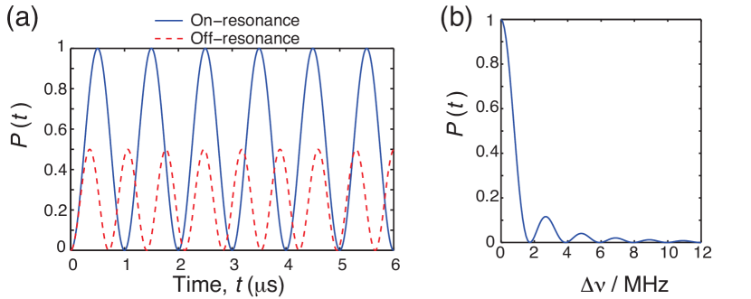
Figure 2.1: (a) Rabi oscillations on- and off-resonance. The vertical axis is the probability $P(t)$ for the electron spin to occupy the higher in energy of its two energy levels and is given by Equation (2.1). The blue line is for the on-resonance case when the excitation and splitting frequencies match ($\nu=\nu_{B}=9\leavevmode\nobreak\ \mathrm{GHz}$). The red line is for off-resonance: $v_{B}$ is increased to $9.001$ GHz. (b) The probability $P(t)$ decays rapidly as a function of the detuning $\Delta\nu\equiv|\nu-\nu_{B}|$. Here, $t$ is fixed to half the time period of on-resonance Rabi osciallations ($0.5\leavevmode\nobreak\ \mu$s).

Coherent quantum control is often demonstrated using a basic CW experiment whereby the qubit is driven between the upper and lower states by continuous excitation and in which so-called Rabi oscillations are observed. For simplicity, we consider an electron initially in the $m_{S}=-1/2$ state. When a sinusoidally oscillating excitation field of frequency $\nu$ is applied, the probability $P(t)$ as a function of time $t$ for the electron to occupy the higher energy state labelled by $m_{S}=+1/2$ is given by

$$P(t)=\left(\frac{\nu_{1}}{\nu_{r}}\right)^{2}\sin^{2}\{\pi\nu_{r}\left(t-t_{0}\right)\},$$ (2.1)

where $\nu_{r}$ is the Rabi frequency:

$$\nu_{r}^{2}=\nu_{1}^{2}+\left(\nu-\nu_{B}\right)^{2},$$ (2.2)

$\nu_{1}$ is the amplitude of the excitation field in frequency units and $\nu_{B}$ is the frequency difference between the two electronic spin states.

The probability $P(t)$ is plotted in Figure 2.1 for an excitation field of amplitude $\nu_{1}=1\leavevmode\nobreak\ \mathrm{MHz}$. Figure 2.1(a) compares the probability for the on-resonance case for which $\nu=\nu_{B}=9\leavevmode\nobreak\ \mathrm{GHz}$ and the case for off-resonance with a finite frequency difference or detuning $\Delta\nu\equiv|\nu-\nu_{B}|=1$ MHz. The probability for the on-resonance case always reaches unity. As the frequency difference $\Delta\nu\equiv|\nu-\nu_{B}|$ is increased, moving away from resonance, the maximum probability drops and the Rabi frequency increases. The sharp drop in the maximum $P(t)$ as we move away from resonance is illustrated in Figure 2.1(b). Whether on- or off-resonance, decoherence damps Rabi oscillations.

2.2 Measuring Coherence Times

The magnetic resonance experiments in which coherence times are measured involve special pulse sequences which we now describe. The simplest of these is the free induction decay (FID), in which a pulse is applied to flip spins in an initially polarised sample to create superpositions of two of the eigenstates. The corresponding polar flip angle from either pole of the Bloch sphere to the equator gives the pulse its name: $\pi/2$-pulse. After the system evolves in time, the $xy$-plane or in-plane magnetisation of the sample is measured and is proportional to the coherence. The Hahn spin echo involves a sequence with one refocusing or $\pi$-pulse and can be classified as the lowest order dynamical decoupling sequence which is applied to extend coherence times before making the measurement to determine $T_{2}$. Higher-order dynamical decoupling sequences apply a train of more than one such refocusing pulses.

2.2.1 Free Induction Decay

The simplest way of measuring the spin coherence time $T_{2}$ is to prepare the desired state of the qubit using an excitation pulse of the correct duration, then leave it to evolve freely in its environment. If the qubit is initially polarised in state $\left|{u}\right\rangle$ or $\left|{l}\right\rangle$, the normalised state after the $\pi/2$-pulse will be the superposition

$$\left|{\psi}\right\rangle=\frac{1}{\sqrt{2}}\left(\left|{u}\right\rangle+e^{i\phi}\left|{l}\right\rangle\right).$$ (2.3)

After a period of free evolution of duration $t$ in the qubit’s environment, the off-diagonal of the (reduced) qubit density matrix is proportional to

$$\left\langle{\hat{\sigma}^{+}}\right\rangle\equiv\left\langle{\hat{\sigma}^{x}}\right\rangle+i\left\langle{\hat{\sigma}^{y}}\right\rangle,$$ (2.4)

in which the expectation values are evaluated in the final state immediately before measurement. The signal in the FID experiment of a single qubit is proportional to this quantity. For measurements on an ensemble of $N$ qubits, the in-plane macroscopic magnetisation vector is the measured quantity:

$${\bf M}_{xy}\propto\sum_{n=1}^{N}\left(\left\langle{\hat{\sigma}^{x}}\right\rangle_{n}\hat{\bf x}+\left\langle{\hat{\sigma}^{y}}\right\rangle_{n}\hat{\bf y}\right)$$ (2.5)

for the uniform magnetic field along $\hat{\bf z}$ as usual. Experimentally, it is possible to distinguish between the $\hat{\bf x}$ and $\hat{\bf y}$ components, but the coherence is often quoted as the magnitude of ${\bf M}_{xy}$. Note that the polarisation of the sample, for example when making a measurement to determine $T_{1}$, is related to ${\bf M}_{z}$. Finally, even for a single qubit, experiments are often repeated and a time average over initial states of the bath is reported.

We are mainly concerned with the single-spin FID which is the intrinsic coherence time of a single central spin system. In measurements of ensembles of such systems, the FID $T_{2}$ time is usually dominated by static inhomogeneous magnetic field broadening from multiple qubits, and is often quoted as $T_{2}^{*}$. The latter coherence time is far shorter than the intrinsic coherence time $T_{2}$.

2.2.2 Hahn Spin Echo

The Hahn spin echo (Hahn, 1950) sequence removes qubit noise originating from static magnetic fields. This includes the inhomogeneous field broadening responsible for the short $T_{2}^{*}$ ensemble coherence time described above. Following a $\pi/2$-pulse, the qubit is allowed to evolve for some time period $\tau$ after which a $\pi$- or refocusing pulse is applied to rotate the state by $180^{\circ}$ about an axis perpendicular to the Bloch vector on the equator. After a further period $\tau$ of free evolution, a spin echo is observed with intensity proportional to the coherence. The pulse sequence is illustrated in Figure 2.2. To measure the coherence time, the sequence is performed for a range of increasing $\tau$, and coherence decay is obtained as a function of $t=2\tau$. The time taken to apply the refocusing times is much shorter than $\tau$, and in most theoretical analyses, the refocusing pulse is assumed to be instantaneous.

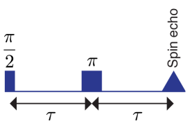
Figure 2.2: The Hahn echo sequence applies a $\pi/2$-pulse followed by free evolution of time duration $\tau$. The refocusing $\pi$-pulse follows and a spin echo is observed after a further time period of $\tau$. To measure the coherence time $T_{2}$, the sequence is repeatedly performed by varying $\tau$ and the in-plane magnetisation observed (at the echo time) as a function of $t=2\tau$.

2.2.3 Carr-Purcell-Meiboom-Gill Sequence

The dynamical decoupling sequence we study is the Carr-Purcell-Meiboom-Gill (CPMG) (Carr and Purcell, 1954; Meiboom and Gill, 1958; Witzel and Das Sarma, 2007a) sequence, which applies a set of $N$ periodically spaced near-instantaneous refocusing pulses (CPMG$N$) as illustrated in Figure 2.3. The Hahn spin echo sequence corresponds to CPMG1. The CPMG sequence is capable of removing noise from time-fluctuating magnetic fields. The frequency of noise removed depends on $N$ or the interval between refocusing pulses $2\tau$. The experiment to measure $T_{2}$ is repeated by varying $\tau$ and decoherence is observed as a function of $t=2\tau N$.

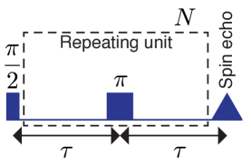
Figure 2.3: The CPMG dynamical decoupling sequence consists of the initial $\pi/2$ pulse, followed by the $-\tau-\pi-\tau-$ sequence repeated $N$ times, after which an echo is observed.

Measured coherence times we compare our theories with are either for the Hahn spin echo or higher-order CPMG sequences on an ensemble of central spin systems. Nevertheless, we also analyse the simpler single-spin FID which is relevant for single-spin experiments (not $T_{2}^{*}$) and compare it with the Hahn echo. We also derive our analytical $T_{2}$ formula for nuclear spin diffusion for the case of the single-spin FID, and numerically account for the effect of the Hahn spin echo.

2.3 Spin Bath Decoherence

The decay in coherence of a central spin system interacting with a bath of other spins can be related to its entanglement with the bath (Breuer and Petruccione, 2002; Witzel et al., 2005; Yao et al., 2006; Liu et al., 2007; Yang and Liu, 2008a). In this section, we describe the problem of central spin decoherence, as illustrated in Figure 2.4.

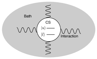
Figure 2.4: Central spin decoherence of a system interacting with a far larger environment or bath. The central system (CS) need not be a spin-1/2 with two energy levels and in general is formed out of two eigenstates of a complex spin Hamiltonian (i.e. a transition between upper and lower levels $\left|{u}\right\rangle\to\left|{l}\right\rangle$).

Consider closed system-bath dynamics governed by total Hamiltonian

$$\hat{H}_{\text{tot}}=\hat{H}_{\text{CS}}+\hat{H}_{\text{int}}+\hat{H}_{\text{bath}}.$$ (2.6)

Here, $\hat{H}_{\text{CS}}$ denotes the central spin (or qubit) Hamiltonian completely isolated from the environment. All system-bath interaction terms are included in $\hat{H}_{\text{int}}$, while the bath degrees of freedom, including intra-bath couplings (essential for decoherence) are contained in $\hat{H}_{\text{bath}}$ (Figure 2.4).

Suppose that at some initial time $t_{0}$ the central system’s state is prepared in a coherent superposition of a pair of its energy eigenstates ($\left|{u}\right\rangle$ and $\left|{l}\right\rangle$). For example, this is the case after applying a $\pi/2$-pulse in a FID or Hahn spin echo experiment. Immediately after preparing the state, we assume that the qubit and bath are in a product state (i.e. unentangled). The combined initial system-bath state is thus

$$\left|{\psi(t_{0})}\right\rangle=\frac{1}{\sqrt{2}}\left(\left|{u}\right\rangle+\left|{l}\right\rangle\right)\otimes\left|{\mathcal{B}(t_{0})}\right\rangle,$$ (2.7)

where the initial bath state is $\left|{\mathcal{B}(t_{0})}\right\rangle$.

Now suppose that the system evolves under $\hat{H}_{\text{tot}}$ (Equation (2.6)) until time $t$ according to the time-dependent Schrödinger equation

$$i\frac{d}{dt}\left|{\psi(t-t_{0})}\right\rangle=\hat{H}_{\text{tot}}\left|{\psi(t-t_{0})}\right\rangle$$ (2.8)

with $\hbar=1$. The formal solution is $\left|{\psi(t-t_{0})}\right\rangle=\hat{U}(t-t_{0})\left|{\psi(t_{0})}\right\rangle$ with the unitary free evolution operator given by

$$\hat{U}(t-t_{0})=e^{-i\hat{H}_{\text{tot}}(t-t_{0})},$$ (2.9)

for time-independent Hamiltonians. The unitary evolution operator $\hat{U}$ may also represent a dynamical decoupling sequence. For example, for the Hahn spin echo we have

$$\hat{U}(t)=e^{-i\hat{H}_{\text{tot}}t/2}\hat{\Pi}e^{-i\hat{H}_{\text{tot}}t/2}.$$ (2.10)

where for simplicity we have chosen $t_{0}=0$. The free evolution, can be written as follows:

$$e^{-i\hat{H}_{\text{tot}}t/2}=\sum_{n}\left|{\phi_{n}}\right\rangle e^{-iE_{n}t/2}\left\langle{\phi_{n}}\right|,$$ (2.11)

after performing the eigendecomposition of the Hamiltonian $\hat{H}_{\text{tot}}$ to obtain the energy eigenbasis $\{\left|{\phi_{n}}\right\rangle\}$ with eigenvalues $\{E_{n}\}$. Assuming the time taken for the $\pi$-pulse is much shorter than $t$, the $\pi$-pulse operator is given by

$$\hat{\Pi}=\left(\hat{\sigma}^{x}+\sum_{n\neq u,l}\left|{n}\right\rangle\left\langle{n}\right|\right)\otimes\hat{\mathds{1}}_{\mathcal{B}},$$ (2.12)

where $\hat{\mathds{1}}_{\mathcal{B}}$ denotes the bath identity and $\hat{\sigma}^{x}$ is the Pauli-$X$ gate $\left|{u}\right\rangle\left\langle{l}\right|+\left|{l}\right\rangle\left\langle{u}\right|$.

After evolution to time $t$, the central system and bath states are in general entangled. Writing the combined system-bath density operator $\hat{\rho}(t)=\left|{\psi(t)}\right\rangle\left\langle{\psi(t)}\right|$, the coherence of the system is characterised by the off-diagonal of its reduced density matrix:

$$\rho_{\text{CS}}^{+-}(t)=\left\langle{u}\right|\text{Tr}_{\mathcal{B}}\left[\hat{\rho}(t)\right]\left|{l}\right\rangle=\left\langle{u}\right|\left(\sum_{k}\left\langle{k}\right|\hat{\rho}(t)\left|{k}\right\rangle\right)\left|{l}\right\rangle,$$ (2.13)

which is obtained by tracing out the bath degrees of freedom; the $\{\left|{k}\right\rangle\}$ here form an orthonormal basis for the bath. The quantity of interest is the off-diagonal

$$\mathcal{L}(t)=\rho_{\text{CS}}^{+-}(t)/\rho_{\text{CS}}^{+-}(0),$$ (2.14)

normalised such that $\mathcal{L}(t=t_{0}=0)\equiv 1$. For this initial time, the phase information contained in the initial state of the system is fully known. The normalization to unity is important for the formulation of the cluster correlation expansion as described in Section 2.5. The coherence $\mathcal{L}(t)$ is proportional to $\left\langle{\hat{\sigma}^{\pm}}\right\rangle\equiv\left\langle{\hat{\sigma}^{x}}\right\rangle\pm i\left\langle{\hat{\sigma}^{y}}\right\rangle$. The density operator is Hermitian, so it does not matter which off-diagonal ($\rho_{\text{CS}}^{+-}\propto\left\langle{\sigma^{+}}\right\rangle$ or $\rho_{\text{CS}}^{-+}\propto\left\langle{\sigma^{-}}\right\rangle$) we consider. Importantly, $|\mathcal{L}(t)|$ is proportional to the signal in an experiment probing the transverse magnetisation.

2.3.1 Initial Bath State

Since nuclear bath energies in a magnetic field $B$ typically exceed intra-bath interaction strengths, we assume a thermal initial state of the bath (unentangled) (Witzel, 2007):

$$\hat{\rho}_{\mathcal{B}}(t_{0})=\sum_{n}P_{n}\left|{\mathcal{B}_{n}(t_{0})}\right\rangle\left\langle{\mathcal{B}_{n}(t_{0})}\right|\simeq\bigotimes_{n}\left(\sum_{m}p_{nm}\left|{b_{nm}}\right\rangle\left\langle{b_{nm}}\right|\right),$$ (2.15)

where $\left|{b_{nm}}\right\rangle$ are eigenstates of the bath Hamiltonian excluding intra-bath interaction terms $\hat{H}^{0}_{\text{bath}}$. For thermal equilibrium,

$$\hat{\rho}_{\mathcal{B}}(t_{0})\approx\exp{\left[-\frac{\hat{H}^{0}_{\text{bath}}}{k_{B}T}\right]},$$ (2.16)

where $k_{B}$ is the Boltzmann constant. Assuming the high-$T$ limit, which is valid for the energies of $\hat{H}^{0}_{\text{bath}}$ and the temperatures we consider, the initial bath density matrix reduces to the identity; i.e. for a given $n$, the states $\left|{b_{nm}}\right\rangle$ occur with equal probability $p_{nm}$.

We note that for small baths, whether for ensemble measurements or single spins, the coherence can be sensitive to sampling from the initial ensemble (Yang and Liu, 2009) and the use of a randomly chosen pure state of the bath is not valid. However, the baths we consider in general consists of a very large number of spins ($\gg 10^{4}$) and for such sufficiently large baths, it is valid to consider a pure initial bath states chosen at random with equal probability amongst the energy eigenstates of $\hat{H}^{0}_{\text{bath}}$. Nevertheless, we consider the case of averaging the complex coherence over such random initial pure states, both for time-averaged measurements and measurements on ensembles of qubits. In the latter case, not only the bath states vary for a single realisation, but also for bath spin positions.

2.3.2 Pure Dephasing

If we assume that during the combined system-bath free evolution the states of the CS remain unchanged, the final state can be written as

$$\left|{\psi(t)}\right\rangle=\frac{1}{\sqrt{2}}\left(e^{-iE_{u}t}\left|{u}\right\rangle\otimes\left|{\mathcal{B}_{u}(t)}\right\rangle+e^{-iE_{l}t}\left|{l}\right\rangle\otimes\left|{\mathcal{B}_{l}(t)}\right\rangle\right).$$ (2.17)

Here, it is clear that the central system and bath are in general entangled and that the bath evolves differently $\left|{\mathcal{B}_{u/l}(t)}\right\rangle$ depending on the state of the system $\left|{u}\right\rangle/\left|{l}\right\rangle$. The phases $e^{-iE_{u/l}t}$ are physically not important as they disappear when we take the modulus of $\mathcal{L}(t)$.

It is easy to show that tracing over the bath and taking the off-diagonal of the resulting reduced density matrix is equivalent to evaluating the overlap between the bath states correlated with the upper and lower system states:

$$\mathcal{L}(t)\propto\langle\mathcal{B}_{u}(t)|\mathcal{B}_{l}(t)\rangle=\langle\mathcal{B}(0)|\hat{T}_{u}^{\dagger}\hat{T}_{l}|\mathcal{B}(0)\rangle.$$ (2.18)

The measured temporal coherence decays can be simulated if one can accurately calculate this overlap. Even for extremely large baths, the initial bath states are the usual thermal states. Thus, the challenge is to evaluate the unitaries $\hat{T}_{u}$ and $\hat{T}_{l}$.

For our systems of interest, the pure dephasing model (i.e. keeping only interaction and bath terms which don’t depolarise the states of the central system) is justified since the energies of the system dominate over typical system-bath and intra-bath couplings. Note that in contrast to the case of an electronic spin-$1/2$ qubit, for the mixed spin qubits which we describe in Chapter 3, if the coherence is evaluated by directly evolving the total Hamiltonian in Equation (2.6), the depolarising terms are not just those involving $\hat{S}^{x}$ and $\hat{S}^{y}$, but also $\hat{S}^{z}$.

2.4 Spin Diffusion

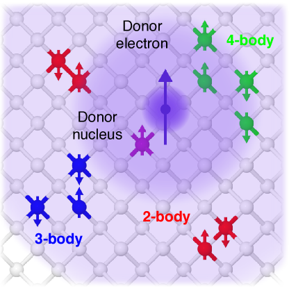
Figure 2.5: Coherences of the central electronic spins are dephased primarily by a surrounding quantum bath of clusters of 2, 3, 4 or more nuclear spin impurities (for natural silicon, pictured) or other donors (for isotopically enriched silicon). Figure adapted from Balian et al. (2015).

We now introduce the mechanism which dominates decoherence in silicon and also in diamond at cryogenic temperatures (i.e. assuming $T$ is small enough such that $T_{1}\gg T_{2}$, which is satisfied when $T<15$ K or so). Nuclear spin diffusion is the process by which a central electronic spin in a solid decoheres due to a nuclear spin bath (de Sousa and Das Sarma, 2003b; Witzel et al., 2005; Yao et al., 2006; Witzel and Das Sarma, 2006). The term spectral diffusion is also used to describe the same process. The problem can be adapted to cases when the central spin and the bath are of the same species and the underlying physics of the process is the same (Witzel et al., 2010, 2012). The following discussion concerns nuclear spin diffusion which is often the case encountered in our decoherence studies, and we use the term spin diffusion to refer to the general problem regardless of the nature of the central system or spin bath.

In nuclear spin diffusion, bath spins are coupled via the magnetic dipole interaction, for example, between ²⁹Si nuclei in silicon or ¹³C nuclei in diamond, both spin-1/2 species. The scenario of a donor qubit in silicon is illustrated in Figure 2.5. In natural silicon, the fractional abundance of ²⁹Si is $f_{\text{natSi}}=0.0467$ (de Sousa and Das Sarma, 2003b). The bath Hamiltonian is a sum over nuclear Zeeman and dipolar Hamiltonians

$$\hat{H}_{\text{bath}} = \hat{H}_{\text{D}}+\hat{H}_{\text{NZ}},$$

$$\hat{H}_{\text{NZ}} = \sum_{n}\hat{H}_{\text{NZ}}^{(n)},\quad\hat{H}_{\text{NZ}}^{(n)}=\gamma_{n}B\hat{I}_{n}^{z},$$

$$\hat{H}_{\text{D}} = \sum_{n<m}\hat{H}_{\text{D}}^{(nm)},\quad\hat{H}_{\text{D}}^{(nm)}=\hat{{\bf I}}_{n}\cdot\mathcal{D}({\bf r}_{nm})\cdot\hat{{\bf I}}_{m},$$ (2.19)

where the bath spins $\hat{{\bf I}}_{n}$ have nuclear gyromagnetic ratios $\gamma_{n}$, $\mathcal{D}$ is the dipolar tensor and ${\bf r}_{nm}$ is the separation vector between localized nuclear spins labelled $n$ and $m$. The Zeeman and dipolar interactions are discussed in Section 2.4.1 and Section 2.4.2 respectively. The central spin system interacts with the bath spins primarily through the electron-nuclear hyperfine interaction:

$$\hat{H}_{\text{int}}=\hat{H}_{\text{HF}}=\sum_{n}\hat{H}_{\text{HF}}^{(n)},\quad\hat{H}_{\text{HF}}^{(n)}=\hat{{\bf S}}\cdot\mathcal{J}({\bf r}_{en})\cdot\hat{{\bf I}}_{n},$$ (2.20)

where $\hat{{\bf S}}$ represents the central electron, $\mathcal{J}$ is the hyperfine tensor described in Section 2.4.3, and ${\bf r}_{en}$ is the electron-nuclear separation. Although anisotropic terms in the interaction Hamiltonian modulate the coherence (Witzel et al., 2007), they have little effect on the $T_{2}$ timescale. Therefore, the isotropic hyperfine interaction can be assumed:

$$\hat{H}_{\text{int}}\simeq\sum_{n}J_{\text{F}}({\bf r}_{n})\hat{{\bf S}}\cdot\hat{{\bf I}}_{n}=\sum_{n}J_{\text{F}}({\bf r}_{n})\left[\hat{S}^{z}\hat{I}_{n}^{z}+\frac{1}{2}(\hat{S}^{+}\hat{I}_{n}^{-}+\hat{S}^{-}\hat{I}_{n}^{+})\right],$$ (2.21)

where $J_{\text{F}}$ is the strength of the Fermi contact interaction which depends on the nuclear position ${\bf r}_{n}$, and is described in Section 2.4.3. We refer to any terms involving a product of two $z$-spin projections as an ‘Ising term’, such as the first term in the square brackets on the R.H.S. of Equation (2.21).

Due to the disparity between the nuclear Zeeman energies and typical dipolar couplings, the dipolar interaction is usually assumed to be secular as described in Section 2.4.2. The secular dipolar interaction includes only terms containing $\hat{I}^{z}_{n}\hat{I}^{z}_{m}$ and $\hat{I}^{+}_{n}\hat{I}^{-}_{m}+\hat{I}^{-}_{n}\hat{I}^{+}_{m}$. The latter term is why the phrase ‘flip-flopping’ spins is used to describe such bath dynamics. Nuclear spin diffusion with an Ising-only hyperfine interaction is further referred to as ‘indirect flip-flops’, to distinguish it from the $T_{1}$-like process of ‘direct flip-flops’ which involves the flip-flop of a bath spin with the central spin (Tyryshkin et al., 2012).

Most of our results are presented for indirect flip-flops in a nuclear spin bath. However, these results are easily generalizable, especially in the context of mitigating decoherence driven by indirect flip-flops in a bath which has the same spin species as the central spin system; for example, in isotopically enriched samples where the abundance of ²⁹Si is reduced (Witzel et al., 2010, 2012; Tyryshkin et al., 2012).

2.4.1 Zeeman Interaction

For simplicity, we begin by describing the Zeeman interaction of a magnetic field with a single electron spin in vacuum (Schweiger and Jeschke, 2001; Weil and Bolton, 2007). Consider an electron in a static and uniform magnetic field $\bm{B}$ which we choose along the $z$-axis. Associated with the electron is the intrinsic angular momentum $\hbar\bm{S}$ called spin. Due to spin and the non-zero electronic charge $e$, the electron possesses a non-zero magnetic dipole moment $\bm{\mu}$ given by

$$\bm{\mu}=\frac{e}{2m_{e}}\hbar\bm{S},$$ (2.22)

where $m_{e}$ is the electronic mass and $\hbar\bm{S}$ is the spin angular momentum vector. The component of $\hbar\bm{S}$ along $z$ is quantized: it can take either one of the values $m_{S}\hbar=\pm\frac{1}{2}\hbar$. Thus, the component of $\bm{\mu}$ along $z$ is

$$\mu_{z}=\gamma_{e}\hbar m_{S},$$ (2.23)

where the constant of proportionality $\gamma_{e}=e/2m_{e}$ is the electron gyromagnetic ratio. Defining the Bohr magneton as $\beta_{e}\equiv|e|\hbar/2m_{e}$ and including the $g$-factor for the free electron $g_{e}$ needed to relate its magnetic moment to an angular momentum in quantum theory, Equation (2.23) becomes

$$\mu_{z}=-g_{e}\beta_{e}m_{S}$$ (2.24)

where the free electron $g$-factor is measured to be $g_{e}=2.0023193043617(15)$ and is well predicted by quantum electrodynamics. Note that this value is for the electron in vacuum and in a solid $g_{e}$ in general is different.

The energy $U$ of a magnetic dipole moment $\bm{\mu}$ in a magnetic field $\bm{B}$ is given by,

$$U=-\bm{\mu}\cdot\bm{B}$$ (2.25)

and for a single electron, this becomes

$$U=-\mu_{z}B=g_{e}\beta_{e}Bm_{S}.$$ (2.26)

The two levels, labelled by $m_{S}=\pm 1/2$, are referred to as the electronic Zeeman energies, and the energy splitting field $\bm{B}$ is sometimes called the Zeeman field. For a transition between the two states, the frequency $\nu$ of an excitation field $\bm{B}_{1}$ inducing the transition must match the energy difference $\Delta U$ between the two states (i.e. $h\nu=\Delta U=g_{e}\beta_{e}B$). By treating the electron as a classical magnetic dipole moment in a static magnetic field, it can be shown that the electron precesses about the field with frequency $\nu_{B}$, a process known as Larmor precession:

$$\nu_{B}=g_{e}\beta_{e}B/h.$$ (2.27)

The Zeeman Hamiltonian describing the response of a general spin $\hat{{\bf S}}$ in ${\bf B}$ is written

$$\hat{H}_{\text{Z}}=\gamma{\bf B}\cdot\hat{{\bf S}},$$ (2.28)

with gyromagnetic ratio $\gamma$ and we have set $\hbar=1$. At this point, we note that all our energies are in angular frequency units of rad s^-1 ($\hat{H}\rightarrow\frac{\hat{H}}{\hbar}$) unless otherwise indicated. In some cases, angular frequency units are scaled by $1/2\pi$, and this is indicated using frequency units Hz.

Choosing ${\bf B}$ along the $z$-axis, $\hat{H}_{\text{Z}}=\gamma B\hat{S}^{z}$. For spin-1/2 species, $\hat{\bf S}=\hat{\bm{\sigma}}/2$, where $\hat{\bm{\sigma}}\equiv(\hat{\sigma}^{x},\hat{\sigma}^{y},\hat{\sigma}^{z})$ is the three-vector of Pauli operators (Appendix B). The gyromagnetic ratios for a donor electron in silicon and a ²⁹Si impurity, both spin-1/2 species, are given in Table 2.1. The nuclear gyromagnetic ratios of Group V donors in silicon are given in Table 3.1. The sign of $\gamma$ determines whether the classical magnetic moment associated with the spin precesses in the clockwise or anticlockwise direction about the magnetic field.

Spin species	$\gamma$ (M rad s-1 T-1)
Electron in silicon	$+1.7591\times 10^{5}$
29Si nucleus	$+53.1903$

Table 2.1: Gyromagnetic ratios $\gamma$ for a donor electron in silicon (Feher, 1959) and a ²⁹Si nucleus (Stone, 2005).

2.4.2 Dipolar Interaction

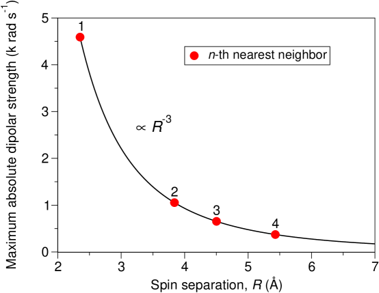
Figure 2.6: The magnitude of the secular dipolar coupling, shown here between two ²⁹Si nuclei with gyromagnetic ratio $\gamma=53.1903$ M rad s^-1 T^-1, falls as the cube of the separation $R$ between the interacting spins. Here, the crystal orientation is such that the direction of the magnetic field is parallel to the line connecting the two spins (i.e. $\theta=0$). The red dots with integer labels mark the strengths for the 1st to 4th nearest neighbor distances in the silicon crystal structure (Appendix C). The nearest neighbor distances are $\tfrac{\sqrt{3}}{4}a_{0}$,$\tfrac{\sqrt{2}}{2}a_{0}$,$\tfrac{\sqrt{11}}{4}a_{0}$ and $a_{0}$ respectively, with lattice parameter $a_{0}=5.43$ Å.

The magnetic dipole interaction (Schweiger and Jeschke, 2001) between two localized spins $\hat{\bf I}_{n}$ and $\hat{\bf I}_{m}$ with gyromagnetic ratios $\gamma_{n}$ and $\gamma_{m}$ is

$$\hat{H}_{\text{D}}^{(nm)}=\hat{{\bf I}}_{n}\cdot\mathcal{D}({\bf r}_{nm})\cdot\hat{{\bf I}}_{m},$$ (2.29)

where ${\bf r}_{nm}$ denotes the relative position vector of the two spins and the components of the dipolar tensor are given by

$$\mathcal{D}_{ij}({\bf r}_{nm})=\frac{\mu_{0}}{4\pi r_{nm}^{3}}\gamma_{n}\gamma_{m}\hbar\left(\delta_{ij}-3\frac{r_{nm}^{(i)}r_{nm}^{(j)}}{r_{nm}^{2}}\right),$$ (2.30)

where $\mu_{0}=4\pi\times 10^{-7}$ NA^-2 is the permeability of free space, $\delta_{ij}$ the Kronecker delta and $i,j=x,y,z$.

In a sufficiently strong and uniform magnetic field, the dipolar interaction can be simplified by keeping only secular or energy conserving terms:

$$\hat{H}_{\text{D}}^{(nm)}\simeq C_{nm}\hat{I}^{z}_{n}\hat{I}^{z}_{m}-\frac{C_{nm}}{4}\left(\hat{I}^{+}_{n}\hat{I}^{-}_{m}+\hat{I}^{-}_{n}\hat{I}^{+}_{m}\right),$$ (2.31)

with strength $C_{nm}$ given by:

$$C_{nm}=\frac{\mu_{0}}{4\pi}\gamma_{n}\gamma_{m}\hbar\frac{(1-3\cos^{2}{\theta_{nm}})}{r_{nm}^{3}}.$$ (2.32)

Here, $\theta_{nm}$ is the angle between the line connecting the spins and the $z$-axis.

For coupling among nuclear spins in the silicon spin bath, the dipolar strength is at most a few k rad s^-1. Since the gyromagnetic ratios of these nuclei are of order tens of M rad s^-1 T^-1, the secular approximation is justified for magnetic field strengths as weak as about 100 mT (Witzel and Das Sarma, 2008).

In order to illustrate the radial dependence of the dipolar interaction, the absolute of the maximum strength (i.e. $|C(\theta=0)|(R)$) is plotted in Figure 2.6 as a function of separation distance $R$ between a pair of ²⁹Si nuclei. For ²⁹Si, the value of $\gamma_{n}$ is given in Table 2.1.

2.4.3 Hyperfine Interaction

Figure 2.7: Isotropic hyperfine couplings (Fermi contact only) for a bismuth donor electron in silicon interacting with a ²⁹Si impurity, as a function of distance between the donor and the impurity. The donor is situated at the origin and the $z=0$ plane is shown. Including spins in the white box is enough for obtaining convergent coherence decays for nuclear spin diffusion using the cluster correlation expansion. The black square (of side length $5.43$ Å) represents the conventional cubic cell of the diamond cubic crystal structure.

The magnetic interaction between an electron $\hat{\bf S}$ and localized nuclei $\hat{\bf I}_{n}$ is essentially given by Equation (2.29). However, due to the spatial extent of the electron wavefunction in a solid, such as in the case of a donor electron, we evaluate

$$\hat{H}_{\text{HF}}^{(n)}=\left\langle{\Psi({\bf r}_{e})}\right|\hat{{\bf I}}_{n}\cdot\mathcal{D}({\bf r}_{en})\cdot\hat{{\bf S}}\left|{\Psi({\bf r}_{e})}\right\rangle=\int d^{3}r_{e}|\Psi({\bf r}_{e})|^{2}\hat{{\bf I}}_{n}\cdot\mathcal{D}({\bf r}_{en})\cdot\hat{{\bf S}},$$ (2.33)

where ${\bf r}_{en}={\bf r}_{e}-{\bf r}_{n}$ is the electron-nuclear separation (de Sousa and Das Sarma, 2003b). In other words, the electron’s position is taken into account by evaluating the expectation value of the interaction in the electron wavefunction $\Psi({\bf r}_{e})$ in real space. This integral has a singularity at ${\bf r}_{en}={\bf 0}$, or when the electron is at the nuclear site. The singularity gives rise to the Fermi contact interaction:

$$J_{\text{F}}({\bf r}_{n})=\frac{2}{3}\gamma_{e}\gamma_{n}\hbar\mu_{0}\left|\Psi({\bf r}_{n})\right|^{2},$$ (2.34)

where $\gamma_{e}$ ($\gamma_{n}$) is the electronic (nuclear) gyromagnetic ratio. Importantly, the Fermi contact interaction only contains the nuclear position ${\bf r}_{n}$ and the origin of the coordinate system is at ${\bf r}_{en}={\bf 0}$. The full interaction is expressed using the hyperfine tensor $\mathcal{J}$ which is decomposed into the Fermi contact and a residual dipolar interaction:

$$\hat{H}_{\text{HF}}^{(n)}=\hat{{\bf I}}_{n}\cdot\mathcal{J}({\bf r}_{en})\cdot\hat{{\bf S}}=J_{\text{F}}({\bf r}_{n})\delta_{ij}+\left\langle\Psi({\bf r}_{e})\left|\mathcal{D}_{ij}({\bf r}_{n})\right|\Psi({\bf r}_{e})\right\rangle.$$ (2.35)

The Fermi interaction is isotropic and the anisotropic dipolar part is effective for nuclei at sufficiently large distances from the origin, where the electron can be assumed localized. Due to the large mismatch between electronic and nuclear gyromagnetic ratios and a sufficiently strong magnetic field, the hyperfine interaction above can be written in secular form and keeping only an Ising term (de Sousa and Das Sarma, 2003b):

$$\hat{H}_{\text{HF}}^{(n)}\simeq\left[J_{\text{F}}({\bf r}_{n})-\frac{\mu_{0}}{4\pi}\gamma_{n}\gamma_{e}\hbar\frac{(1-3\cos^{2}{\theta_{n}})}{r_{n}^{3}}\Theta(r_{n}-r_{0})\right]\hat{S}^{z}\hat{I}_{n}^{z},$$ (2.36)

where $r_{n}\equiv|{\bf r}_{n}|$ and $\Theta(r_{n}-r_{0})$ is the Heaviside step function; i.e. the electron-nuclear residual dipolar interaction is non-zero for $r>r_{0}$ (for donors in silicon, $r_{0}\approx 20$ Å).

The Kohn-Luttinger donor electronic wavefunction (de Sousa and Das Sarma, 2003b) is often employed for the silicon donors, to evaluate the probability density at the nuclear site $|\Psi({\bf r}_{n})|^{2}$. The wavefunction is derived from effective mass theory. It leads to oscillations and near-exponential decay of the hyperfine contact strength according to

$$J_{\text{F}}({\bf r})=\frac{4}{9}\gamma_{e}\gamma_{n}\hbar\mu_{0}\left[F_{1}({\bf r})\cos{(k_{0}x)}+F_{2}({\bf r})\cos{(k_{0}y)}+F_{3}({\bf r})\cos{(k_{0}z)}\right]^{2}$$ (2.37)

where ${\bf r}\equiv{\bf r}_{n}=(x,y,z)$, $k_{0}=(0.85)2\pi/a_{0}$ and $\gamma_{e}$ is the electron gyromagnetic ratio in silicon. The cubic lattice parameter is $a_{0}$ (see Appendix C for the silicon crystal structure) and $\eta$ is the charge density on each crystal site. The relevant envelope functions are:

$$F_{1}({\mathbf{r}})=\frac{\exp{\left[-\sqrt{\frac{x^{2}}{(nb)^{2}}+\frac{y^{2}+z^{2}}{(na)^{2}}}\right]}}{\sqrt{\pi(na)^{2}(nb)}},$$ (2.38)

$$F_{2}({\mathbf{r}})=F_{1}({\mathbf{r}})\text{\leavevmode\nobreak\ with\leavevmode\nobreak\ }\{x\to y,y\to z,z\to x\},$$ (2.39)

$$F_{3}({\mathbf{r}})=F_{1}({\mathbf{r}})\text{\leavevmode\nobreak\ with\leavevmode\nobreak\ }\{x\to z,y\to x,z\to y\},$$ (2.40)

where $a$ and $b$ are lengths characteristic to the donor and $n=\sqrt{0.029\leavevmode\nobreak\ \text{eV}/\epsilon_{i}}$ with the electron ionization energy $\epsilon_{i}$ in eV.

Numerical values for a Group V donor in silicon interacting with ²⁹Si impurities are given in Table 2.2. Calculated couplings using the values in Table 2.2 are plotted in Figure 2.7 as a function of distance from the donor electron. The electronic and nuclear gyromagnetic ratios are given in Table 2.1, the silicon lattice constant is $a_{0}=5.43$ Å and the ionization energies of the Group V donors in silicon are in Table 3.1.

Parameter	Value
Charge density $\eta$	186
Length $a$	$25.09$ Å
Length $b$	$14.43$ Å

Table 2.2: Numerical values for calculating the hyperfine interaction between a donor electron spin in silicon and a ²⁹Si spin impurity (de Sousa and Das Sarma, 2003b).

We note that for our calculations the residual dipolar interaction in Equation (2.35) is assumed to be secular and only becomes effective after a distance of $na$ from the origin. The value of $na$ is about 20 Å for silicon donors.

2.4.4 Hyperfine-Mediated Interaction

The hyperfine-mediated interaction (also known as the RKKY interaction) (Yao et al., 2006; Liu et al., 2007), is a long-range coupling between two nuclear spins mediated by an electron hyperfine-coupled to each of the two nuclei. It results from the flip-flop part of $\hat{\bf I}\cdot\hat{\bf S}$ terms in the hyperfine interaction in Equation (2.35). For a pair of nuclei, using perturbation theory, it can be approximated as

$$\hat{H}_{\text{RKKY}}^{(nm)}\simeq-\frac{J_{\text{F},n}J_{\text{F},m}}{4\gamma_{e}B}\left(\hat{I}_{n}^{+}\hat{I}_{m}^{-}+\hat{I}_{n}^{-}\hat{I}_{m}^{+}\right)\hat{S}_{z}.$$ (2.41)

For decoherence of hybrid qubits, the intra-bath dipolar interaction dominates over the RKKY. Also, for the case of the Hahn echo, it is suppressed. However, the RKKY becomes important when considering nuclear spin decoherence in Chapter 8.

We now proceed to explain the CCE for approximating the many-body dynamics of a central spin system in a spin bath. The CCE has been extensively applied for both nuclear spin diffusion (see e.g. Balian et al. (2014)) and spin diffusion due to an all-dipolar electron spin system (see e.g. Witzel et al. (2012)).

2.5 Cluster Correlation Expansion

As stated in Chapter 1, it is not in practice possible to exactly solve for the dynamics for tens of thousands of bath spins. For spin baths with strong back action with the qubit, cluster expansion methods (Witzel et al., 2005; Witzel and Das Sarma, 2006; Yang and Liu, 2008a, b, 2009; Witzel et al., 2012) have enabled realistic numerical simulations of the joint system-bath dynamics, predicting coherence times in remarkable agreement with experiment (see e.g. Balian et al. (2014) or Ma et al. (2014)). Here we describe the most general of these – the cluster correlation expansion (CCE) (Yang and Liu, 2008a, b, 2009). The CCE also happens to have the simplest formulation which we outline in this section.

In the CCE and analogous formalisms, $\hat{H}_{\text{tot}}$ is diagonalised for sets or ‘clusters’ of bath spins of varying sizes up to some maximum cut-off size and the coherence decay is obtained from a product over all cluster contributions in the bath. Clusters are illustrated for the case of the hybrid qubit in silicon in Figure 2.5.

2.5.1 General Formalism

We first derive the CCE and later discuss its physical motivation. We wish to calculate the complex coherence function $\mathcal{L}(t)$ as a function of time $t$ (regardless of any dynamical decoupling pulses). Let the set of all spins in the bath be denoted by $\mathcal{R}$, and write the exact coherence as $\mathcal{L}_{\mathcal{R}}(t)\equiv\mathcal{L}(t)$. This quantity results from exactly solving the closed system-bath dynamics, then tracing out the entire bath to obtain the off-diagonal of the reduced density matrix of the central system. Even for tens of spins in the bath, this problem is practically impossible on a classical supercomputer.

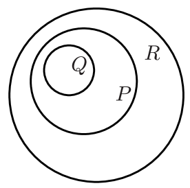
Figure 2.8: The CCE decomposes the set of all bath spins $\mathcal{R}$ into all its subsets or ‘clusters’ of spins: $\dots\subseteq\mathcal{Q}\subseteq\mathcal{P}\subseteq\mathcal{R}$.

We now decompose the bath into all its subsets or clusters $\mathcal{P}$, as illustrated in Figure 2.8, and note that these subsets include $\mathcal{R}$, the entire bath itself. For a given $\mathcal{P}$, the coherence $\mathcal{L}_{\mathcal{P}}(t)$ is evaluated by considering the central system and bath spins contained only in $\mathcal{P}$. This defines the reduced problem for $\mathcal{P}$. In other words, the reduced problem for $\mathcal{P}$ has all bath spins outside of $\mathcal{P}$ completely “frozen”.

We now expand the reduced problem for $\mathcal{L}_{\mathcal{P}}(t)$ as a product of cluster correlation terms $\tilde{\mathcal{L}}_{\mathcal{P}}(t)$:

$$\mathcal{L}_{\mathcal{P}}(t)=\prod_{\mathcal{Q}}\tilde{\mathcal{L}}_{\mathcal{Q}}(t).$$ (2.42)

Equation (2.42) essentially defines the CCE. The cluster correlation or ‘tilde’ terms are defined recursively by re-writing Equation (2.42),

$$\mathcal{L}_{\mathcal{P}}(t) = \prod_{\mathcal{Q}\subseteq\mathcal{P}}\tilde{\mathcal{L}}_{\mathcal{Q}}(t)$$ (2.43)

$$= \tilde{\mathcal{L}}_{\mathcal{P}}(t)\prod_{\mathcal{Q}\subset\mathcal{P}}\tilde{\mathcal{L}}_{\mathcal{Q}}(t),$$

hence,

$$\tilde{\mathcal{L}}_{\mathcal{P}}(t)=\frac{\mathcal{L}_{\mathcal{P}}(t)}{\prod_{\mathcal{Q}\subset\mathcal{P}}\tilde{\mathcal{L}}_{\mathcal{Q}}(t)}.$$ (2.44)

Thus, the cluster correlation term for the cluster of spins $\mathcal{P}$ is given by solving for $\mathcal{L}_{\mathcal{P}}(t)$ and recursively dividing by lower order correlations formed by $\mathcal{Q}$, the proper subsets of $\mathcal{P}$. Once all the cluster correlation terms are obtained, $\mathcal{L}_{\mathcal{R}}(t)\equiv\mathcal{L}(t)$ is exactly recovered using the CCE:

$$\mathcal{L}_{\mathcal{R}}(t)=\prod_{\mathcal{P}}\tilde{\mathcal{L}}_{\mathcal{P}}(t).$$ (2.45)

As it stands, the exact CCE (Equation (2.45)) seems practically useless because the correlation term for $\mathcal{R}$ contains the exact solution $\mathcal{L}_{\mathcal{R}}$. The strength of the CCE method becomes evident when the expansion is truncated to include subsets bound by the number of spins they contain:

$$\mathcal{L}_{[k]}(t)=\prod_{|\mathcal{P}|\leq k}\tilde{\mathcal{L}}_{\mathcal{P}}(t).$$ (2.46)

2.5.2 Convergence and Heuristics

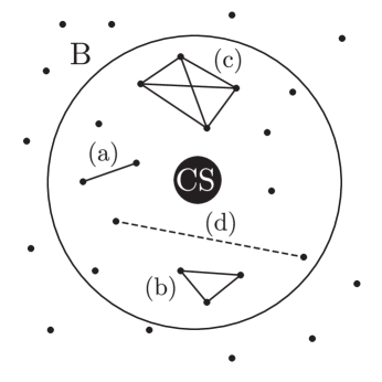
Figure 2.9: ‘CS’ denotes the central spin system or qubit, in its environment, or bath ‘B’ of interacting spins. Clusters of 2 (a), 3 (b) and 4 (c) spins are depicted, with all intra-bath interactions shown as lines connecting the spins. There are no clusters outside the sphere around the qubit, and clusters which include spins far away from one another are excluded (d).

Equation (2.46) is the $k$-th order truncation to the CCE (which we denote by CCE$k$) and includes clusters for no more than $k$ spins in each cluster. The expansion’s success is judged by its convergence with respect to $k$, and also how small $k$ is. The CCE can be said to be converged at $k=k^{\prime}$ when $|\mathcal{L}_{[k^{\prime}]}(t)-\mathcal{L}_{[k^{\prime}+1]}(t)|,|\mathcal{L}_{[k^{\prime}]}(t)-\mathcal{L}_{[k^{\prime}+2]}(t)|,\dots,\ll 1,\forall t$. For example, if there is little difference in the coherence decay for CCE2 and the decays for CCE3 and CCE4, then the CCE is reasonably converged at $k=2$. Also, the practicality of the CCE is limited by the order of convergence.

Whether or not the CCE converges and the order of convergence depend on the relative interaction strengths in the bath and interaction Hamiltonians. Practically, heuristic cut-offs are also imposed. For example, the dipolar interaction decays as the inverse cube of the inter-spin separation. Therefore, only spins separated by some cut-off distance are allowed to form clusters as the contribution from farther away spins is relatively negligible. Also, for nuclear spin diffusion, the extent of the electronic wavefunction imposes a radial cut-off for the superlattice cube or sphere in which clusters are formed. Heuristic cut-offs are illustrated in Figure 2.9.

2.5.3 Physical Motivation

The product of coherences in the CCE is motivated by the fact that for two clusters $\mathcal{A}$ and $\mathcal{B}$ that are sufficiently far apart so that the interactions between spins in $\mathcal{A}$ and those in $\mathcal{B}$ are negligible compared to interactions inside the individual clusters, it can be shown that the combined coherence is well approximated by the product $\mathcal{L}_{\mathcal{AB}}\simeq\mathcal{L}_{\mathcal{A}}\mathcal{L}_{\mathcal{B}}$. The task is to compute the correction $\mathcal{L}_{\text{corr}}$ as the interactions between $\mathcal{A}$ and $\mathcal{B}$ are increased, in order to obtain the exact value of $\mathcal{L}_{\mathcal{AB}}$:

$$\mathcal{L}_{\mathcal{AB}}=\mathcal{L}_{\mathcal{A}}\mathcal{L}_{\mathcal{B}}\mathcal{L}_{\text{corr}}.$$ (2.47)

For simplicity, consider three spins labelled 1, 2 and 3 and assume that the lowest-order contribution to the coherence is pairwise flip-flops, given by $\mathcal{L}_{(1,2)}\mathcal{L}_{(1,3)}\mathcal{L}_{(2,3)}$. The correction required to take into account collective many-body flip-flops is simply

$$\mathcal{L}_{\text{corr}}=\frac{\mathcal{L}_{(1,2,3)}}{\mathcal{L}_{(1,2)}\mathcal{L}_{(1,3)}\mathcal{L}_{(2,3)}}\equiv\tilde{\mathcal{L}}_{(1,2,3)},$$ (2.48)

giving the true or non-factorisable 3-body correlation which we denote using $\tilde{\mathcal{L}}_{(1,2,3)}$. Since the lowest-order correlations in this example are from two-clusters, the true non-factorizable correlation equals the in general factorizable correlation: $\tilde{\mathcal{L}}_{(i,j)}=\mathcal{L}_{(i,j)}$. Thus, for many pairs and triplets in the bath, the coherence is given by

$$\mathcal{L}=\prod_{(i,j)}\tilde{\mathcal{L}}_{(i,j)}\prod_{(i,j,k)}\tilde{\mathcal{L}}_{(i,j,k)}.$$ (2.49)

Equation (2.49) motivates the systematic expansion Equation (2.45), which takes into account $n$-body correlations.

2.5.4 Beyond the Standard CCE

The discussion so far has not made any reference to the initial state of the bath. For a pure product initial state, the reducible correlation terms $\mathcal{L}(t)$ for each cluster are calculated by simply considering a product state of eigenstates of the non-interacting bath $\hat{H}^{0}_{\text{bath}}$. For relatively small baths, the coherence calculated can be highly sensitive to initial state sampling. Also, for a non-factorizable or entangled initial bath states, the CCE described above is not valid. The ensemble-averaged CCE has been developed for these reasons (Yang and Liu, 2009). However, these cases are not encountered in our work and the quantities of interest are largely insensitive to the choice of initial product bath states we use.

Another important modification of the CCE exists (Witzel et al., 2010, 2012) in which Ising interactions with spins external to each cluster are included in addition to the usual interactions within the cluster. In addition, an efficient method of averaging over initial bath states has been developed (Witzel et al., 2012). These modifications were required to speed up convergence and to remove numerical instabilities for the all-dipolar problem of a central electron spin interacting with an electron spin bath.

Finally, we note that the expansion need not formally be a product expansion. In fact, the CCE has been reformulated using sums and differences of correlation terms (Witzel et al., 2014b).

2.5.5 Pair Correlations

The lowest non-trivial CCE order for spin diffusion is $k=2$ or CCE2. This only involves the qubit-bath dynamics involving pairs of spins in the bath – pair correlations.

If a pure dephasing model is assumed, as described in Section 2.3.2, the bath dynamics is governed by effective Hamiltonians depending on the state of the central system. In other words, the total Hamiltonian has a form such that terms depending on the states of the central system are uncoupled. These state-dependent uncoupled Hamiltonians are:

$$\hat{h}_{i}\equiv\left\langle{i}\right|(\hat{H}_{\text{int}}+\hat{H}_{\text{bath}})\left|{i}\right\rangle,$$ (2.50)

written for state $\left|{i}\right\rangle$.

An orthonormal basis for two spin-1/2 particles is $\left|{\uparrow\uparrow}\right\rangle,\left|{\downarrow\downarrow}\right\rangle,\left|{\uparrow\downarrow}\right\rangle,\left|{\downarrow\uparrow}\right\rangle$. Here, $\left|{\uparrow\downarrow}\right\rangle\equiv\left|{\uparrow}\right\rangle\otimes\left|{\downarrow}\right\rangle$, where $\left|{\uparrow/\downarrow}\right\rangle$ denotes spin up/down. Therefore, the state-dependent Hamiltonians above act on this basis. Furthermore, for a secular flip-flop intra-bath interaction, the only matrix elements involved in the interaction are those involving the states $\left|{\uparrow\downarrow}\right\rangle$ and $\left|{\downarrow\uparrow}\right\rangle$. The other two polarised states only contribute a phase factor which disappears when the modulus of the coherence is taken. Note that care must be taken when averaging over initial bath states and coherences of unity in this model must be accounted for the polarised states. The state-dependent Hamiltonians can be written using $2\times 2$ matrices in the basis $\{\left|{\uparrow\downarrow}\right\rangle$ , $\left|{\downarrow\uparrow}\right\rangle\}$:

$$\hat{h}_{i}=a\hat{\mathds{1}}+b\hat{\bm{\sigma}}\cdot{\bf H}_{i},$$ (2.51)

where $\hat{\bm{\sigma}}$ is the three-vector of Pauli operators and ${\bf H}_{i}$ is an effective field about which these so-called ‘pseudospins’ precess. The length of the state-dependent pseudofields gives the pseudospin precession frequency and is obtained by diagonalising Equation (2.51). The identity term in Equation (2.51) is dynamically uninteresting, contributing a constant shift to the pseudospin energies. This central state-dependent dynamics has been applied for a variety of spin problems including quantum dots and NV centres (Yang and Liu, 2008a, b, 2009; Yao et al., 2006, 2007; Liu et al., 2007; Zhao et al., 2012a), the latter involving one-spin cluster dynamics at the lowest non-trivial order.

2.5.6 Many-Body Correlations

We use the term ‘many-body or $n$-body correlations’ to refer to qubit-bath dynamics containing non-negligible contributions from clusters including more than two bath spins ($n>2$). For example, in spin diffusion, collective flip-flops of three bath spins are referred to as to 3-body correlations. It is of fundamental interest to isolate such many-body correlations (Ma et al., 2014; Balian et al., 2015). These are rare occurrences, and most of the decoherence problems in this thesis are described by only considering pair correlations (or CCE2). However, we shall see that near an OWP and for low to moderate pulsed dynamical decoupling, 3-body clusters dominate the dynamics.

2.6 Conclusion

In conclusion, the current chapter primarily serves as a resource for understanding our theoretical results in subsequent chapters dealing with decoherence. The basic principles of magnetic resonance, in particular experiments measuring coherence times were outlined. The problems of central spin decoherence and spin diffusion were introduced and finally, we described the CCE for solving for the many-body qubit-bath dynamics. In summary, here we have described $\hat{H}_{\text{bath}}$ and $\hat{H}_{\text{int}}$. In the next chapter, we discuss $\hat{H}_{\text{CS}}$ for the hybrid qubit.

3  |  The Hybrid Qubit

This chapter primarily concerns the central spin Hamiltonian $\hat{H}_{\text{CS}}$ for our central spin decoherence problem with total Hamiltonian given by Equation (2.6). The central system we consider is in general a mixed electron-nuclear or ‘hybrid’ qubit.

It is often the case that magnetic resonance transitions are between states which are eigenstates of the magnetic field or Zeeman Hamiltonian described in Section 2.4.1. The central Hamiltonian may, for example, contain multiple uncoupled spins. The basis of eigenstates in this case is the product of states labelled by the magnetic quantum numbers (of $z$-projection spin operators) of the non-interacting spin species. The term ‘mixed’ here refers to the case when the eigenstates can no longer be approximated using these Zeeman states, but instead involve their entanglement.

Electronic spin manipulation times are much shorter compared to those of nuclear spins. For the hybrid qubit, however, we show that an NMR transition in the high-field limit can be manipulated on short ESR timescales in the mixing regime. For quantum information applications, the shortest manipulation time and longest coherence time are highly desirable. The coherence times of the hybrid qubit are the topic of Chapter 5 for the Hahn spin echo and Chapter 7 for higher orders of dynamical decoupling.

In what follows, we present the spin Hamiltonian of the hybrid qubit and its eigendecomposition. Examples are the Group V donors in silicon, in particular bismuth donors, due to their exceptionally strong mixing. We then describe fast quantum control of the hybrid qubit, published in Morley et al. (2013). The latter reference also contains numerical simulations of coherence times which we present in Chapter 5, and use to confirm the dominant decoherence mechanism in the experiments of Morley et al. (2013). This study not only demonstrated fast control, but also relatively long coherence times of the hybrid qubit.

3.1 Group V Donors in Silicon

Our hybrid electron-nuclear qubit can be implemented as one of the Group V hydrogenic impurities in silicon. These are phosphorus, arsenic, antimony and bismuth in increasing period of the periodic table. The notation Si:$X$ is used to denote $X$-doped silicon, where $X$ is one of the four donor atoms. Silicon has four valence electrons, thus a Group V impurity donates a single electron which at low enough temperatures is localized at the substitutional site of the donor nucleus (Stoneham, 2001). The host impurity nuclear spin is coupled to the donor electron spin via the isotropic Fermi contact hyperfine interaction (which we describe in detail in Section 2.4.3 for the case of a donor electron and a bath nucleus). Ionization energies of the donors, their nuclear gyromagnetic ratios, nuclear spin quantum numbers and electron-nuclear hyperfine coupling strengths are given in Table 3.1.

Donor $X$	$\epsilon_{i,X}$ (eV)	$\gamma_{X}$ (M rad s-1 T-1)	$I_{X}$	$A_{X}$ (M rad s-1)
Phosphorus 31P	0.044	$-108.41$	1/2	$7.3846\times 10^{2}$
Arsenic 75As	0.049	$-45.95$	3/2	$1.2467\times 10^{3}$
Antimony 121Sb	0.040	$-64.44$	5/2	$1.174\times 10^{3}$
Bismuth 209Bi	0.069	$-43.775$	9/2	$9.2702\times 10^{3}$

Table 3.1: Nuclear gyromagnetic ratios $\gamma_{X}$, donor electron ionization energies $\epsilon_{i,X}$, nuclear spin total quantum numbers $I_{X}$ and isotropic hyperfine coupling strengths $A_{X}$ of the Group V donors in silicon (Si:$X$). Values for $\epsilon_{i,X}$ and $A_{X}$ can be found in Feher (1959) and values for $\gamma_{X}$ and $I_{X}$ in Stone (2005).

3.1.1 Spin Hamiltonian and Eigenspectrum

The effective spin Hamiltonian of a donor in silicon (Si:$X$) in a magnetic field $B$ along the $z$-axis is given by the sum of Zeeman and hyperfine terms (Mohammady et al., 2010, 2012),

$$\hat{H}_{\text{Si:}X}=\omega_{0}\left(\hat{S}^{z}+\delta_{X}\hat{I}^{z}_{X}\right)+A_{X}\hat{{\bf I}}_{X}\cdot\hat{{\bf S}},$$ (3.1)

where the electron Larmor precession frequency is $\omega_{0}=\gamma_{e}B$ and $\gamma_{e}$ is the gyromagnetic ratio of the electron spin in silicon. The hyperfine interaction between the host nuclear and donor electron spins is well-approximated by considering only the isotropic Fermi contact part, here denoted by $A_{X}$, to distinguish it from hyperfine coupling to the bath $J_{\text{F}}$. The nuclear gyromagnetic ratio is contained in $\delta_{X}=\gamma_{X}/\gamma_{e}$, which is much smaller than $\gamma_{e}$ (i.e. $|\delta_{X}|\ll 1$).

For the case of the Zeeman and hyperfine terms having comparable magnitudes ($\omega_{0}\sim A_{X}$), the matrix representation of the Hamiltonian in Equation (3.1) is no longer diagonal in the the Zeeman basis $\left|{m_{S}}\right\rangle\otimes\left|{m_{I}}\right\rangle\equiv\left|{m_{S},m_{I}}\right\rangle$, where $m_{S}=\pm 1/2$ and $m_{I}=-I_{X},-I_{X}+1,\dots,I_{X}$. This competition between the two terms is significant for the donor systems at typical magnetic field strengths for ESR experiments ($B\simeq 0.1-0.6$ T), especially for bismuth which has the largest hyperfine strength.

It is easy to show that the sum of spin $z$-projections commute with the Hamiltonian:

$$\left[\hat{H}_{\text{Si}:X},\hat{S}^{z}+\hat{I}^{z}_{X}\right]=0,$$ (3.2)

and thus a good set of quantum numbers for the eigenbasis of Equation (3.1) are $-|I_{X}+S|,-|I_{X}+S|+1,\dots,I_{X}+S$. These label the mixed or ‘adiabatic’ eigenstates $\left|{\pm,m}\right\rangle$ which mix the Zeeman basis to (at most) doublets of constant $m=m_{S}+m_{I}$ with energies $E^{\pm}_{m}\left(\omega_{0}\right)$. Due to the commutation relation Equation (3.2), the Hamiltonian Equation (3.1) can be divided into two one-dimensional Hamiltonians acting on bases

$$\{\left|{1/2,I_{X}}\right\rangle\},\{\left|{-1/2,-I_{X}}\right\rangle\},$$

and 2$I$ two-dimensional Hamiltonians acting on

$$\{\left|{\pm 1/2,m\mp 1/2}\right\rangle,\left|{\mp 1/2,m\pm 1/2}\right\rangle\},$$

the latter with $|m|\leq I_{X}-1/2$. In other words, in its matrix representation in the Zeeman basis, the Hamiltonian is in block form composed of $2\times 2$ matrices of which there are $2I$ and two $1\times 1$ entries. Eigenstates of the one-dimensional Hamiltonians are those which have $m=\pm|I_{X}+1/2|$ and they remain unmixed at all magnetic field, with energies

$$E_{m=\pm|I_{X}+1/2|}\left(\omega_{0}\right)=\pm\frac{\omega_{0}}{2}(1-2\delta_{X}I_{X})+\frac{A_{X}I_{X}}{2}.$$ (3.3)

The two-dimensional Hamiltonian for each doublet is

$$\hat{H}_{m\neq\pm|I_{X}+1/2|}=\frac{A}{2}\left(R_{m}\cos{\theta_{m}}\hat{\sigma}^{z}+R_{m}\sin{\theta_{m}}\hat{\sigma}^{x}-\epsilon_{m}\hat{\mathds{1}}\right),$$ (3.4)

where

$$\cos\theta_{m} = \frac{\Omega_{m}(\omega_{0})}{R_{m}(\omega_{0})},$$ (3.5)

$$\sin\theta_{m} = \frac{\Delta_{m}}{R_{m}(\omega_{0})},$$ (3.6)

and,

$$R_{m}(\omega_{0})^{2} = \Omega_{m}^{2}(\omega_{0})+\Delta^{2}_{m},$$ (3.7)

$$\Omega_{m}(\omega_{0}) = m+\tilde{\omega}_{0}(1+\delta_{X}),$$ (3.8)

$$\tilde{\omega}_{0} = \frac{\omega_{0}}{A_{X}},$$ (3.9)

$$\Delta^{2}_{m} = (I_{X}+\tfrac{1}{2})^{2}-m^{2},$$ (3.10)

$$\epsilon_{m} = \frac{1}{2}\left(1+4\tilde{\omega_{0}}m\delta_{X}\right).$$ (3.11)

Diagonalising the above Hamiltonian, the eigenstates $\left|{\pm,m}\right\rangle$, mixed in the product Zeeman basis are given by

$$\left|{\pm,m}\right\rangle=a_{m}\left|{m_{S}=\pm\frac{1}{2}}\right\rangle\otimes\left|{m_{I}=m\mp\frac{1}{2}}\right\rangle\pm b_{m}\left|{m_{S}=\mp\frac{1}{2}}\right\rangle\otimes\left|{m_{I}=m\pm\frac{1}{2}}\right\rangle,$$ (3.12)

with amplitudes

$$a_{m} = \cos{\frac{\theta_{m}}{2}},$$ (3.13)

$$b_{m} = \sin{\frac{\theta_{m}}{2}},$$ (3.14)

and corresponding eigenenergies

$$E^{\pm}_{m}\left(\omega_{0}\right)=\frac{A_{X}}{2}\left[-\frac{1}{2}\left(1+4\tilde{\omega}_{0}m\delta_{X}\right)\pm R_{m}(\omega_{0})\right].$$ (3.15)

In the notation $\left|{\pm,m}\right\rangle$, the two unmixed eigenstates are thus $\left|{+,I_{X}+1/2}\right\rangle$ and $\left|{-,-|I_{X}+1/2|}\right\rangle$.

We often write the adiabatic eigenstates using the notation $\left|{i}\right\rangle=1,2,\dots,d$, where $d=(2S+1)(2I_{X}+1)=4I_{X}+2$. The transformations between the two labels $\left|{i}\right\rangle\leftrightarrow\left|{\pm,m}\right\rangle$ are given by,

$$\left|{i}\right\rangle = \left|{{\begin{array}[]{rl}+&\mbox{for $2I_{X}+2\leq i\leq 4I_{X}+2$}\\ -&\mbox{for $1\leq i\leq 2I_{X}+1$}\end{array}},|2I_{X}+1-i|-S-I_{X}}\right\rangle$$ (3.18)

$$\left|{\pm,m}\right\rangle = \left|{{\begin{array}[]{rl}&3I_{X}-S+2+m\\ &S+I_{X}-m\end{array}}}\right\rangle.$$ (3.21)

It is clear that $a_{m}^{2}+b_{m}^{2}=1$ (eigenstates are normalised). The difference $(a_{m}^{2}-b_{m}^{2})$ is proportional to the expectation value of the electron spin $z$-projection,

$$\left\langle{\pm,m}\right|\hat{S}^{z}\left|{\pm,m}\right\rangle=\pm\frac{1}{2}(a_{m}^{2}-b_{m}^{2})=\pm\cos{\theta_{m}}=\frac{\Omega_{m}(\omega_{0})}{R_{m}(\omega_{0})}\equiv\frac{P_{i}(\omega_{0})}{2},$$ (3.22)

half the polarisation $P_{i}(\omega_{0})$ for the $i$-th eigenstate $\left|{i}\right\rangle\equiv\left|{\pm,m}\right\rangle$. For the unmixed system, we take the limit $\omega_{0}\to\infty$ so $R_{m}\to\Omega_{m}$ and the polarisation $\pm 1$ for the bare electron is recovered (i.e. $\langle\hat{S}^{z}\rangle=\pm 1/2$).

3.1.2 Frequency-Field Gradient

Denoting the excitation frequency for the two levels in a transition as $f$, at $df/dB=0$ points, decoherence from classical field noise is significantly reduced (Mohammady et al., 2012). The Hellmann-Feynman theorem (Cohen-Tannoudji et al., 1977) states that the derivative of the energy with respect to some parameter in the Hamiltonian, in this case the magnetic field $B$, is obtained by evaluating the derivative of the expectation value of the Hamiltonian in the corresponding energy eigenstate. Thus,

$$\frac{dE_{i}}{dB} = \left\langle{i}\right|\frac{d\hat{H}_{\text{Si:}X}}{dB}\left|{i}\right\rangle$$ (3.23)

$$= \left\langle{i}\right|\frac{d}{dB}\left(\gamma_{e}B\hat{S}_{z}+\gamma_{X}B\hat{I}^{z}_{X}+A_{X}\hat{{\bf I}}_{X}\cdot\hat{{\bf S}}\right)\left|{i}\right\rangle$$

$$= \gamma_{e}\langle\hat{S}^{z}\rangle_{i}+\gamma_{X}\langle\hat{I}^{z}_{X}\rangle_{i}.$$

The excitation frequency is simply $f=(E_{i=u}-E_{i=l})/2\pi$ for a magnetic resonance transition $\left|{i=u}\right\rangle\to\left|{i=l}\right\rangle$ between an upper ($i=u$) and a lower ($i=l$) level. Therefore, the frequency-field gradient is given by

$$\frac{df}{dB}=\frac{1}{2\pi}\left[\frac{\gamma_{e}}{2}(P_{u}-P_{l})+\gamma_{X}\left(\langle\hat{I}^{z}_{X}\rangle_{u}-\langle\hat{I}^{z}_{X}\rangle_{l}\right)\right],$$ (3.24)

and it can be shown that the $B$ values for which $df/dB=0$, satisfy,

$$0=P_{u}(B)-P_{l}(B)+\frac{\delta_{X}(m_{l}-m_{u})}{1+\delta_{X}},$$ (3.25)

where $m_{u/l}$ are the $m_{S}+m_{I}$ quantum numbers for the two levels.

3.1.3 Cancellation Resonances

When $\Omega_{m}=0$, the polarisation $P_{i}$ vanishes. Also, the $\hat{\sigma}^{z}$ term in Equation (3.4) is zero, and thus the eigenstates become those of $\hat{\sigma}^{x}$:

$$\left|{\Psi^{\pm}}\right\rangle=\frac{1}{\sqrt{2}}\left(\left|{\frac{1}{2},m-\frac{1}{2}}\right\rangle\pm\left|{-\frac{1}{2},m+\frac{1}{2}}\right\rangle\right).$$ (3.26)

Typically, due to the large mismatch between electronic and nuclear gyromagnetic ratios, $\delta_{X}\ll 1$ and hence $\Omega_{m}\simeq m+\tilde{\omega_{0}}$. Thus, the Bell-like eigenstates above occur at magnetic fields corresponding to $\tilde{\omega_{0}}\simeq-m$. For $-(I_{X}-1/2)\leq m\leq 0$, these field values correspond to Landau-Zener (LZ) crossings. The LZ points have OWPs (see below) midway between them in $\theta_{m}$ coordinates. Fields when the doublet Hamiltonian reduces to a sum of $\hat{\sigma}^{z}$ and $\hat{\sigma}^{x}$ with the same coefficients may also be of special interest.

3.1.4 Optimal Working Points

For coupling of the electronic spin to a nuclear spin bath, the OWPs considered in this thesis and discussed in Chapter 5. Chapter 6 and Chapter 7 occur when $P_{u}=P_{l}$ for the transition $\left|{u}\right\rangle\to\left|{l}\right\rangle$. Since typically, $\delta_{X}\ll 1$, some OWP and $df/dB=0$ points (Equation (3.25)), can be extremely close in magnetic field.

3.2 Bismuth Donor

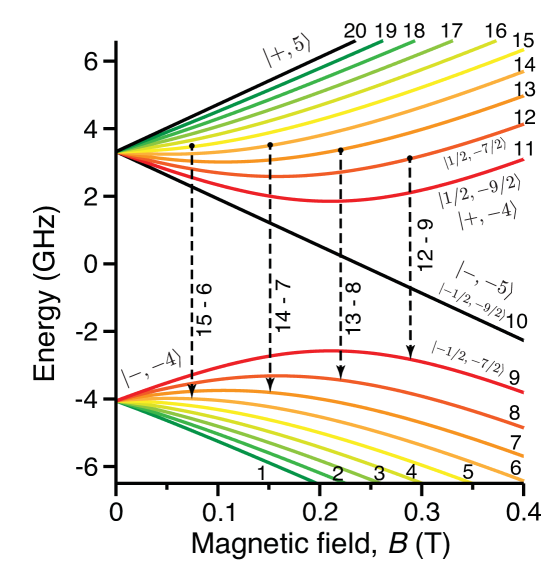
Figure 3.1: The spectra of donor spin systems such as arsenic, antimony or bismuth (pictured) are affected by strong mixing between the electron and host nuclear spin, at magnetic fields $B$ smaller or comparable to the hyperfine coupling $A$, allowing a richer behaviour than unmixed electron spins. The plot shows the eigenspectrum of Si:Bi as a function of magnetic field $B$ labelled in order of increasing energy $\left|{i}\right\rangle$ using integers $1,\dots,20$, in the Zeeman basis $\left|{m_{S}}\right\rangle\otimes\left|{m_{I}}\right\rangle\equiv\left|{m_{S},m_{I}}\right\rangle$ (i.e. as $B\to\infty$) and using the adiabatic basis $\left|{\pm,m}\right\rangle$. Strong mixing of the Zeeman basis is evident in the region $B\simeq 0.1-0.3$ T due to competition between the Zeeman and hyperfine Hamiltonians. At particular field values termed optimal working points (OWPs), decoherence can be strongly suppressed. The arrows indicate the transitions with four of the most significant OWPs. The colours match for the two states in each doublet labelled by $m$. Figure adapted from Mohammady et al. (2010) and Balian et al. (2015).

The bismuth donor is special among the Group V donors in two aspects. First, the hyperfine coupling is the strongest of all the Group V donors (Table 3.1). The large hyperfine value means that there is significant electron-nuclear mixing for fields in the range ‘intermediate ESR field regime’: $B\simeq 0.1-0.6$ T. Second, the bismuth nucleus has the highest dimension of Hilbert space since $I_{\text{Bi}}=9/2$, giving $2(9+1)=20$ energy levels and thus a large number of states for possible manipulation in quantum information applications. The strong hyperfine and large $I_{\text{Bi}}$ lead to the largest number of OWPs among the silicon donors. We note that for an OWP, $I_{X}>1/2$ and hence the Si:P system ($I_{\text{P}}=1/2$) unfortunately does not have any.

3.2.1 Energy Levels and $X$-Band Transitions

The energy spectrum as a function of magnetic field for Si:Bi is shown in Figure 3.1. The eigenstates can be labelled in multiple ways: in order of increasing energy ($\left|{i}\right\rangle$, $i=1,2,\dots,20$), in the Zeeman basis in the high-field limit ($\left|{m_{S},m_{I}}\right\rangle$, $m_{S}=\mp\tfrac{1}{2}$, $m_{I}=-\tfrac{9}{2},-\tfrac{7}{2},\dots,\tfrac{7}{2},\tfrac{9}{2}$), or the adiabatic basis ($\left|{\pm,m}\right\rangle$, $-5\leq m\leq 5$). Since the Zeeman basis is no longer the eigenbasis of the Hamiltonian, the usual ESR and NMR selection rules presented in Chapter 2 do not apply. Nevertheless, we refer to $\left|{\pm,m}\right\rangle\leftrightarrow\left|{\mp,m-1}\right\rangle$ and $\left|{\pm,m}\right\rangle\leftrightarrow\left|{\pm,m-1}\right\rangle$ as ESR-type and NMR-type transitions respectively, noting that $\left|{-,m}\right\rangle\leftrightarrow\left|{+,m-1}\right\rangle$ are dipole forbidden in the high field limit.

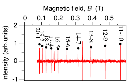
Figure 3.2: Experimental CW ESR spectrum of bismuth-doped silicon at excitation frequency $f=9.7$ GHz (red lines) showing good agreement with the resonance positions predicted by theory (black dots). Ten transitions $\left|{i=u}\right\rangle\to\left|{j=l}\right\rangle$ are observed with $i=11,\dots,20$ and $j=10,\dots,1$ (see horizontal dashed line in Figure 3.3). Figure adapted from Mohammady et al. (2010).

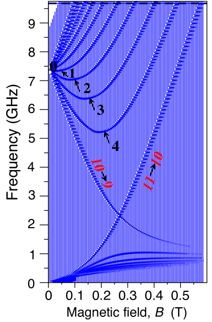
Figure 3.3: ESR excitation frequency $f$ as a function of magnetic field $B$ for bismuth-doped silicon. The $df/dB=0$ extrema correspond to magnetic fields at which classical noise decoherence is significantly reduced. The dashed horizontal line shows the $X$-band excitation frequency at $9.7$ GHz, corresponding to the measured spectrum in Figure 3.2. The labelled transitions are those at $S$-band (4 GHz) and the black integers label the cancellation resonances, where the electronic Zeeman and hyperfine terms cancel in the donor Hamiltonian (Equation (3.1)). Figure adapted from Mohammady et al. (2010).

The CW ESR spectrum for Si:Bi at an excitation frequency of $f=9.7$ GHz ($X$-band) is shown in Figure 3.2 showing 10 spectral lines. This is a region of weak mixing. The resonance positions are in excellent agreement with the analytical expressions for the eigenspectrum described above.

3.2.2 OWPs, CTs and Other Special Fields

The OWPs we consider correspond to suppression of decoherence in quantum spin environments. Si:Bi has four ESR-type and four-NMR type OWPs. These OWPs are all doublets, so there are in fact 16 separate OWP transitions. The OWPs we primarily consider are the ESR-type ones corresponding to states $\left|{12}\right\rangle\to\left|{9}\right\rangle$ and $\left|{14}\right\rangle\to\left|{7}\right\rangle$ occurring at $B\simeq 0.19$ T and $B\simeq 0.08$ T respectively. The transitions corresponding to four ESR-type OWPs are labelled in Figure 3.1, while the other four correspond to forbidden transitions close by. It is important to note that all of these couple two neighbouring avoided crossings. Selection rules are detailed in (Mohammady et al., 2012), but OWP transitions have $\Delta m=\pm 1$ which implies that $\langle u|{\hat{S}}^{z}|l\rangle=0$ meaning that magnetic field fluctuations do not induce bit flips $\left|{u}\right\rangle\leftrightarrow\left|{l}\right\rangle$ (assuming Ising-like coupling to the bath).

An important consequence of the strong mixing in Si:Bi is the existence of multiple $df/dB=0$ maxima and minima in the $f-B$ parameter space. These are shown in Figure 3.3. There are $df/dB=0$ minima for the $|15\rangle\to|6\rangle$, $|14\rangle\to|7\rangle$, $|13\rangle\to|8\rangle$, $|12\rangle\to|9\rangle$, and $|11\rangle\to|8\rangle$ transitions in the frequency range $5-7.5$ GHz and two maxima for $|12\rangle\to|11\rangle$ and $|9\rangle\to|8\rangle$ close to $1$ GHz. The $df/dB=0$ points are referred to as ‘clock transitions’ (CTs) (Wolfowicz et al., 2013) and correspond to where decoherence arising from classical field noise is reduced (Mohammady et al., 2012). They are distinct from the OWP points, albeit in close proximity to them in magnetic field.

One might also consider the possibility of creating a superposition of two states $|u\rangle$ and $|l\rangle$ at a single avoided crossing; for example, the superposition $|11\rangle+|9\rangle$ in Figure 3.1, at the avoided crossing between these states at $B\simeq 0.21$ T. Although the $\left|{11}\right\rangle\to\left|{9}\right\rangle$ transition is never allowed, such a superposition might be created by a two pulse excitation from level $\left|{10}\right\rangle$. Both states are at zero energy gradient ($dE_{u,l}/dB=0$) so coherences are to first order insensitive to dephasing noise; however, as shown in Mohammady et al. (2012), in that case $\langle u|{\hat{S}}^{z}|l\rangle\neq 0$ so magnetic fluctuations couple the states in the superposition and thus coherence is vulnerable to depolarisation by magnetic noise.

The cancellation resonance points are where the hyperfine interaction cancels the Zeeman splitting. They occur for Si:Bi at magnetic fields $\omega_{0}\simeq-mA$ and $m=0,-1,-2,-3,-4$, labelled in Figure 3.3. They correspond to the avoided crossings seen in Figure 3.1. Finally, the field for which $\tilde{\omega_{0}}\simeq 7$ corresponds to $df/dB=0$ maxima CTs and NMR-type OWPs for the $\left|{12}\right\rangle\to\left|{11}\right\rangle$ and $\left|{9}\right\rangle\to\left|{8}\right\rangle$ transitions, and is where the doublet donor Hamiltonian is proportional to $(\hat{\sigma}^{x}+\hat{\sigma}^{z})$.

3.3 Fast Quantum Control

The current section concerns pulsed ESR control of the hybrid qubit on the nanosecond timescale as demonstrated by experiments in Morley et al. (2013). The coherence times for the hybrid qubit for the transitions and magnetic fields at which the experiments were performed are presented in Chapter 5. The experiments presented herein were carried out by Dr. Petra Lueders at ETH Zurich with assistance from Dr. Gavin Morley and Dr. Hamed Mohammady, who are all co-authors of Morley et al. (2013), which is published work co-authored by S.J.B., contributing to the theme of the thesis.

Magnetic resonance involves transitions between doublets adjacent in $m$ (i.e. $m\to m\pm 1$), using the notation of energy states of the hybrid qubit as described above. The usual ESR and NMR selection rules correspond to single electronic and nuclear spin flips respectively as discussed in Section 2.1. These selection rules are in the usual ‘unmixed regime’ or equivalently in the limit of $B\to\infty$. The time taken to manipulate electronic spins by pulsed ESR is often on the order of nanoseconds; much faster than pulsed NMR manipulation of nuclei which typically takes microseconds. This is because the gyromagnetic ratio of the electron is of order GHz T^-1 whereas for nuclei it is on the MHz T^-1 scale. If electrons and nuclei were to be used for quantum information processing, the shortest possible total manipulation time is highly desirable. Importantly, the manipulation time must also be shorter than the coherence time in order to implement quantum error correction protocols.

3.3.1 Forbidden Transitions

An important consequence of the strong mixing for the hybrid qubit (implemented as Si:Bi) is the existence of ESR transitions of its eigenstates which are ESR-forbidden at high fields but can be manipulated using fast ESR pulses in the strong mixing or hybrid regime. Furthermore, as we shall see in Chapter 5, the qubit coherence times in the hybrid regime can be up to five orders of magnitude longer than the manipulation times and are limited by nuclear spin diffusion by a ²⁹Si spin bath. We use the term hybrid because in this regime the electron and nucleus are hybridized (Equation (3.12)) or near 50:50 superpositions of bare electronic and nuclear spin Zeeman states.

3.3.2 $S$-Band Transitions

To access the hybrid regime in Si:Bi, a $4.044$ GHz ESR excitation frequency was used ($S$-band). As can be seen in Figure 3.3, this corresponds to two transitions: $\left|{10}\right\rangle\to\left|{9}\right\rangle$ and $\left|{11}\right\rangle\to\left|{10}\right\rangle$ at $B=145.6$ mT and $B=345.0$ mT respectively. The CW ESR spectrum at this frequency is shown in Figure 3.4, in which the resonance positions are well predicted by analytical diagonalisation (Equation (3.12)) of the donor Hamiltonian (Equation (3.1)).

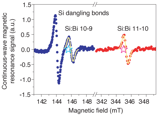
Figure 3.4: Magnetic resonance spectrum of bismuth-doped silicon (Si:Bi) at 4 K with 4.044 GHz CW excitation ($S$-band). The predicted positions of both Si:Bi resonances are shown as stars. The bismuth dopant concentration is about $3\times 10^{15}$ cm^-3 and the magnetic field was perpendicular to the $[111]$ direction of the doped silicon crystal. Figure adapted from Morley et al. (2013).

In the high-field limit at $f\simeq 4$ GHz, the observed transitions are:

$$(\left|{11}\right\rangle\to\left|{10}\right\rangle)_{B\to\infty} \equiv \left|{m_{S}=\frac{1}{2},m_{I}=-\frac{9}{2}}\right\rangle\to\left|{-\frac{1}{2},-\frac{9}{2}}\right\rangle,$$ (3.27)

$$(\left|{10}\right\rangle\to\left|{9}\right\rangle)_{B\to\infty} \equiv \left|{m_{S}=-\frac{1}{2},m_{I}=-\frac{9}{2}}\right\rangle\to\left|{-\frac{1}{2},-\frac{7}{2}}\right\rangle$$ (3.28)

and respect the usual selection rules, the first being an ESR transition and the second an NMR one. Clearly, the second transition violates the ESR selection rule and is not expected to be seen in ESR spectra. This is indeed the case in the high field limit. However, in the hybrid regime, this ESR forbidden transition is observed as shown in Figure 3.4.

The ESR transition amplitudes are given by matrix elements of the electron $x$-spin projection:

$$\left\langle{10}\right|\hat{S}^{x}\left|{9}\right\rangle \propto \sin{\left(\frac{\theta_{-4}}{2}\right)},$$ (3.29)

$$\left\langle{11}\right|\hat{S}^{x}\left|{10}\right\rangle \propto \cos{\left(\frac{\theta_{-4}}{2}\right)}.$$ (3.30)

The states $\left|{11}\right\rangle$ and $\left|{9}\right\rangle$ form the $m=-4$ doublet. For $B=0.15$ T or the $\left|{11}\right\rangle\to\left|{10}\right\rangle$ transition, $\theta_{-4}=0.62\pi$ and for the other transition $\theta_{-4}=0.28\pi$. The ratio of the modulus of the transition amplitudes is therefore

$$\frac{|\left\langle{11}\right|\hat{S}^{x}\left|{10}\right\rangle|}{|\left\langle{10}\right|\hat{S}^{x}\left|{9}\right\rangle|}\simeq 1.1.$$ (3.31)

The Rabi oscillation frequency is proportional to the transition amplitude. Thus, this ratio (in the hybrid regime) predicts the same order of magnitude manipulation for an ESR transition and a (high-field) NMR one. Usually, the Rabi oscillations are 103 times slower for NMR relative to ESR. The transition rate is proportional to the square of the amplitude, hence, this ratio predicts a ratio of magnetic resonance intensities of about $1.1^{2}\approx 1.2$. This calculated value is in agreement with the measured intensities as shown in Figure 3.5.

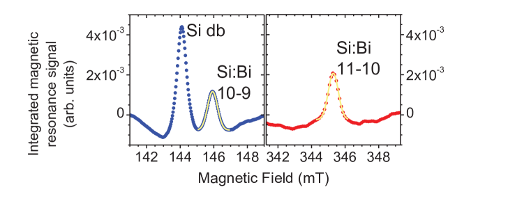
Figure 3.5: The areas under the Gaussians (obtained by integrating the spectra in Figure 3.4) are in the ratio area_11-10/area_10-9 = 1.2, in agreement with calculated values. Figure adapted from Morley et al. (2013).

3.3.3 Rabi oscillations

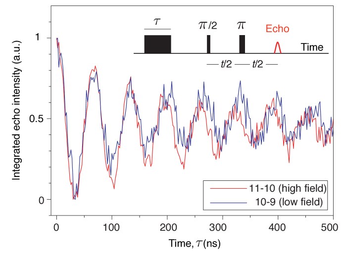
Figure 3.6: Rabi oscillations demonstrate coherent control of both of the 4 GHz hybrid electron-nuclear transitions. At higher magnetic fields, the 11-10 resonance becomes an ESR transition, whereas the 10-9 resonance becomes an NMR transition. Controlling this NMR transition in the past has required $\pi$ pulses of $\geq 4\leavevmode\nobreak\ \mu$s, two orders of magnitude longer than the 32 ns $\pi$ pulses we use here. Figure adapted from Morley et al. (2013).

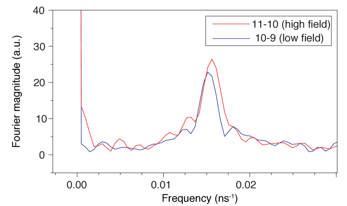
Figure 3.7: . Fourier transforming the Rabi oscillations in Figure 3.6 reveals that the 11-10 transition experiences 10% faster nutation, as expected. Pulsed measurements used 16 ns $\pi/2$ pulses and 32 ns $\pi$ pulses with two-step phase cycling. Figure adapted from Morley et al. (2013).

Rabi oscillations were used to demonstrate coherent control of the hybrid electron-nuclear qubit. The pulse sequence of the experiment is as follows: $\tau-\pi/2-t-\pi-t-\text{echo}$. The experiment varies the first pulse $\tau$, rotating the qubit from the upper towards the lower transition by some polar angle on the Bloch sphere. The lower eigenstate is reached if the angle is $\pi$ and the time taken is the duration of the $\pi$-pulse as described in Chapter 2. The usual Hahn echo experiment follows the first pulse in order to obtain a good signal. The period of Rabi oscillations is simply twice the $\pi$-pulse time. The time taken for the $\pi$-pulse is quoted as the qubit manipulation time.

The Rabi oscillations for the two transitions at 4 GHz are shown in Figure 3.6. The Fourier transformation of the Rabi signal (Figure 3.7) reveals that the inverse of the Rabi frequency is about $1/66$ ns^-1, corresponding to a qubit manipulation time of 32 ns. The ratio of the two Rabi frequencies extracted from the experimental data is about 1.1 and is in agreement with the calculation in Equation (3.31). In the high-field limit, the $\left|{10}\right\rangle\to\left|{9}\right\rangle$ transition would be a pure NMR transition and thus require manipulation times of order microseconds.

3.4 Conclusion

In summary, we introduced the spin Hamiltonian of the hybrid electron-nuclear qubit and analytical expressions for its energies and eigenstates. We then discussed the bismuth donor as a hybrid qubit. The calculated eigendecomposition of the hybrid qubit leads to resonance positions in excellent agreement with experiment at both $X$-band and $S$-band excitation frequencies, commonly used for ESR studies. By accessing ESR-forbidden transitions by operating in the hybrid regime, a factor of $125$ speed-up can be achieved in the qubit manipulation time, from 4 $\mu$s in the high-field limit to 32 ns in the hybrid regime. However, we note that this speed-up is limited by the power of the microwave field driving the transition. The fundamental speed-up, on the other hand, is limited by the ratio of the electronic to host nuclear gyromagnetic ratios, and is a factor of $1/\delta_{\text{Bi}}\approx 4,000$.

4  |  Interaction of Hybrid Qubit
with a Nuclear Spin Bath

The content of this chapter was published in Balian et al. (2012). Here, we present pulsed ENDOR experiments using bismuth-doped silicon which enable us to characterise the coupling between the hybrid qubit and the surrounding spin bath of ²⁹Si impurities. This spin bath provides the dominant decoherence mechanism (nuclear spin diffusion) at low temperatures ($<16$ K) for the hybrid qubit. At magnetic fields corresponding to OWPs, we demonstrate a collapse in the strength of the qubit-bath interaction. This serves as a clear spectroscopic signature of OWPs at which decoherence is suppressed as shown in Chapter 5.

Relevant for decoherence of the hybrid qubit, the experiments suggest that anisotropic hyperfine contributions are comparatively weak, and isotropic couplings dominate; hence anisotropic couplings can be safely neglected in calculating hyperfine couplings for our decoherence simulations. Importantly this means that the form of the suppression of decoherence at OWPs is largely independent of crystal orientation.

The central hybrid qubit is coupled to the ²⁹Si spin bath via the electron-nuclear hyperfine interaction introduced in Section 2.4.3. In general, the hyperfine interaction is in tensor form and includes the effects of both isotropic and anisotropic couplings. Anisotropic couplings depend on the direction of the magnetic field relative to the crystal (or equivalently, the ‘sample orientation’). The crystal structure of silicon is described in Appendix C.

The pulsed ENDOR measurements (as opposed to continuous-wave) also motivate the possibility of addressing nuclear impurity spins for quantum information applications. We present decoherence mechanisms for such spins in Chapter 8.

4.1 Pulsed ENDOR Measurements

The nature of the qubit-bath interaction is investigated by means of pulsed ENDOR (Schweiger and Jeschke, 2001). Previous ENDOR studies of Si:Bi used radio frequencies of at least several hundreds of MHz (Morley et al., 2010; George et al., 2010), and thus could not probe the weak couplings to the nuclear spin bath. In contrast, radio frequencies of a few MHz were used in the work we present. With this approach, we successfully measured the hyperfine couplings of the bismuth donor to ²⁹Si impurities and determined their anisotropy.

The experiments spectroscopically resolve and characterise a set of distinct $\mathcal{J}_{n}$ as defined in Equation (2.35), corresponding to occupancy of inequivalent lattice sites by ²⁹Si impurities, and whether or not these have any anisotropic character.

4.1.1 Experimental Method

Pulsed ENDOR experiments were carried out by Dr. Micha Kunze and Professor Chris Kay at UCL who are co-authors of Balian et al. (2012). The Davies ENDOR pulse sequence was used (Schweiger and Jeschke, 2001), which applies the sequence $\pi_{\text{mw}}-\tau_{1}-\pi_{\text{rf}}-\tau_{2}-\frac{\pi}{2}{\text{\scriptsize mw}}-\tau_{3}-\pi_{\text{mw}}-\tau_{3}-\text{echo}$, where the microwave frequency (mw) is chosen to excite one ESR transition and the radio frequency (rf) is stochastically varied between $2-12$ MHz or $2-7$ MHz to excite all nuclear spin transitions in this region. $256$ ns long $\pi_{\text{mw}}$-pulses and a $128$ ns long $\frac{\pi}{2}{\text{\scriptsize mw}}$-pulse were used. For optimal signal-to-noise ratio and resolution, a $\pi_{\text{rf}}$-pulse of $10\leavevmode\nobreak\ \mu\text{s}$ was used. Pulse delays were set to $\tau_{1}=1\leavevmode\nobreak\ \mu\text{s}$, $\tau_{2}=3\leavevmode\nobreak\ \mu\text{s}$, and $\tau_{3}=1.5\leavevmode\nobreak\ \mu\text{s}$ and a shot repetition time of 1.3 ms was employed to give a good signal-to-noise ratio. All experiments were carried out at 15 K on an E580 pulsed EPR ($\equiv$ESR) spectrometer (Bruker Biospin) equipped with pulsed ENDOR accessory (E560D-P), a dielectric ring ENDOR resonator (EN4118X-MD4), a liquid helium flow cryostat (Oxford CF935), and a radio frequency amplifier (ENI A-500W). The donor concentration of the sample was $3\times 10^{15}$ cm^-3 and the magnetic field was directed perpendicular to the $(111)$ crystal plane.

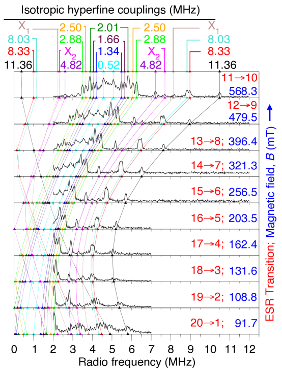
Figure 4.1: Pulsed ENDOR measured for bismuth-doped silicon with frequency 9.8 GHz at which ten ESR lines are observed, the resonance peaks due to interactions of the donor with ²⁹Si nuclei at inequivalent lattice sites. The isotropic hyperfine couplings were extracted from the spectrum at the highest magnetic field. As the field is varied, the smooth lines follow the resonance positions according to Equation (4.10). Solid and dotted lines distinguish between the two peaks observed for each coupling, each corresponding to one of the two donor levels involved in the ESR transition. Only the peaks labelled $X_{1}$ and $X_{2}$, in addition to a third pair not resolved here, were found to show anisotropy from performing ENDOR as a function of crystal orientation. Figure adapted from Balian et al. (2012).

4.1.2 Experimental Results

While not offering the higher frequency resolution attainable with CW ENDOR (Feher, 1959; Hale and Mieher, 1969a, b), the pulsed ENDOR measurements permit us to adequately constrain calculated hyperfine couplings and thus demonstrate the reliability of our numerical simulations of $T_{2}$. In particular, we established that isotropic couplings to the spin bath dominate over anisotropic ones. As mentioned above, a further motivation for pulsed experiments in contrast to CW is to investigate the feasibility of an alternative possibility for QIP: to simultaneously manipulate the ²⁹Si spins as spin-1/2 qubits, along with the donors (Akhtar et al., 2012). Measured ENDOR spectra at ESR excitation frequency $f\simeq 9.755$ GHz are presented in Figure 4.1, together with a list of the extracted qubit-bath hyperfine couplings.

4.2 Calculating Resonance Positions

For the magnetic field range $B\simeq 0.1-0.6$ T in Figure 4.1, there is significant mixing of the high-field Si:Bi energy eigenstates (Figure 3.1). We now proceed to derive an expression for the ENDOR resonance positions, taking into account the effect of the central-state mixing. We note that in Equation (2.35) describing the hyperfine interaction in Section 2.4.3, the Fermi contact part is always isotropic. The remainder of the interaction has both anisotropic and isotropic components. Here, since we are interested in measurements of the interaction, we make no reference to the Fermi contact part of the interaction and instead divide the tensor into isotropic and anisotropic components. Also, since we are measuring the interaction, there is no need to write down the spatial electronic wavefunction.

4.2.1 Hyperfine Tensor

To investigate the qubit-bath interaction, we add to the central spin Hamiltonian the interaction Hamiltonian and a single spin-$1/2$ ²⁹Si nuclear Zeeman term:

$$\hat{H}_{\text{ENDOR}}=\hat{H}_{\text{Si:Bi}}+\gamma_{n}B\hat{I}^{z}+\hat{{\bf I}}\cdot\mathcal{J}\cdot\hat{{\bf S}},$$ (4.1)

where $\mathcal{J}$ here is the hyperfine tensor for coupling to a single ²⁹Si nucleus and $\gamma_{n}$ is the ²⁹Si gyromagnetic ratio given in Table 2.1. The donor Hamiltonian $\hat{H}_{\text{Si:Bi}}$ is given by Equation (3.1). Interactions of ²⁹Si nuclei at different lattice sites with the same donor electron can be treated by summing independent such hyperfine terms:

$$\hat{H}_{\text{int}}=\hat{H}_{\text{Si:Bi}}+\sum_{l}\left(\gamma_{n}B\hat{I}_{l}^{z}+\hat{{\bf I}}_{l}\cdot\mathcal{J}_{l}\cdot\hat{{\bf S}}\right).$$ (4.2)

Nuclear ²⁹Si–²⁹Si and ²⁰⁹Bi–²⁹Si dipolar interactions are much weaker and thus negligible compared to the electron-nuclear hyperfine interaction. This is because the latter involves the product of electronic and nuclear gyromagnetic ratios which is $\sim 1000$ stronger than a product of two nuclear gyromagnetic ratios as seen from Table 2.1 and Table 3.1.

The hyperfine tensor is diagonal in the molecular frame (MF); this coordinate system is one in which the external field direction is collinear with the line connecting the central bismuth and ²⁹Si sites (Schweiger and Jeschke, 2001):

$$\mathcal{J}^{\text{MF}}=\left(\begin{array}[]{ccc}a_{\text{iso}}-T&0&0\\ 0&a_{\text{iso}}-T&0\\ 0&0&a_{\text{iso}}+2T\\ \end{array}\right),$$ (4.3)

where $T$ and $a_{\text{iso}}$ are scalars. Rotating the operator $\left(\hat{{\bf I}}\cdot\mathcal{J}\cdot\hat{{\bf S}}\right)^{\text{MF}}$ by angle $\theta$ towards the laboratory $z$-axis (along $B$), where $\theta$ is the angle between the $z$-axis and the line connecting the ²⁹Si spin and the donor site in the molecular frame, gives $\left(\hat{{\bf I}}\cdot\mathcal{J}\cdot\hat{{\bf S}}\right)$ in the laboratory frame in terms of $T$, $a_{\text{iso}}$ and the rotation angle $\theta$:

$$\hat{H}_{\text{ENDOR}}=\hat{H}_{\text{Si:Bi}}+\gamma_{n}B\hat{I}^{z}+\alpha\hat{I}^{z}\hat{S}^{z}+\beta\hat{I}^{x}\hat{S}^{z},$$ (4.4)

where

$$\alpha = \left[\left(a_{\text{iso}}-T\right)+3T^{2}\cos^{2}\theta\right],$$

$$\beta = 3T\sin\theta\cos\theta,$$ (4.5)

and we have ignored non-secular terms involving $\hat{S}^{x}$ and $\hat{S}^{y}$. This secular approximation which reduces the hyperfine interaction to the simpler form above is motivated by the disparity between the central spin (electronic Zeeman and host hyperfine) and donor-²⁹Si hyperfine energy scales. Non-secular terms lead to transitions between ESR levels. To simulate the ENDOR resonance positions, we wish to describe nuclear transitions (MHz) for each of the two ESR levels (GHz) independently. The Hamiltonian above appears in Schweiger and Jeschke (2001) and the term $\hat{S}^{z}\hat{I}^{y}$ vanishes if we choose the ²⁹Si nucleus to lie in the $xz$-plane.

4.2.2 Expression for Resonance Positions

For a transition between the central spin states $\left|{u}\right\rangle\to\left|{l}\right\rangle$, we choose the basis formed by the states

$$\begin{array}[]{rl}\left|{u}\right\rangle&\otimes\leavevmode\nobreak\ \leavevmode\nobreak\ \left|{\uparrow}\right\rangle,\\ \left|{u}\right\rangle&\otimes\leavevmode\nobreak\ \leavevmode\nobreak\ \left|{\downarrow}\right\rangle,\\ \left|{l}\right\rangle&\otimes\leavevmode\nobreak\ \leavevmode\nobreak\ \left|{\uparrow}\right\rangle,\\ \left|{l}\right\rangle&\otimes\leavevmode\nobreak\ \leavevmode\nobreak\ \left|{\downarrow}\right\rangle,\end{array}$$ (4.6)

where $\left|{\uparrow}\right\rangle$ ($\left|{\downarrow}\right\rangle$) is the spin up (down) eigenstate of the non-interacting ²⁹Si spin-1/2. The matrix representation of the $4\times 4$ Hamiltonian in this basis is

$$\begin{split}{\bf H}_{\text{ENDOR}}&=\left(\begin{array}[]{ccc}{\bf h}_{u}&{\bf 0}\\ {\bf 0}&{\bf h}_{l}\end{array}\right)\\ {\bf h}_{u/l}&=\left(\begin{array}[]{ccc}E_{u/l}+\frac{\gamma_{n}B}{2}+\frac{\alpha P_{u/l}}{4}&\frac{\beta P_{u/l}}{4}\\ \frac{\beta P_{u/l}}{4}&E_{u/l}-\frac{\alpha P_{u/l}}{4}-\frac{\alpha P_{u/l}}{4}\end{array}\right)\end{split}$$ (4.7)

where $E_{u/l}$ are the energies of the central states $\left|{u}\right\rangle/\left|{l}\right\rangle$. Straightforward diagonalisation of ${\bf h}_{u/l}$ gives the expression for the ENDOR resonance frequency at ESR level $\left|{i}\right\rangle,i=u,l$, written in units of Hz:

$$\Delta f^{(i)}=\frac{1}{2\pi}\sqrt{\left(\frac{\gamma_{n}B}{2}\omega_{0}+\frac{\alpha_{\perp}P_{i}(B)}{4}\right)\sin^{2}\theta+\left(\frac{\gamma_{n}B}{2}\omega_{0}+\frac{\alpha_{\parallel}P_{i}(B)}{4}\right)\cos^{2}\theta},$$ (4.8)

with $\alpha_{\parallel}$ and $\alpha_{\perp}$ given by

$$\begin{split}\alpha&=\alpha_{\parallel}\cos^{2}\theta+\alpha_{\perp}\sin^{2}\theta,\\ \alpha_{\parallel}&=a_{\mathrm{iso}}+2T,\\ \alpha_{\perp}&=a_{\mathrm{iso}}-T.\end{split}$$ (4.9)

Note that in the case when there is no angular dependence of an ENDOR line (i.e. $T=0$), Equation (4.9) reduces to

$$\Delta f_{\text{iso},l}^{(i)}(B)=\frac{1}{2\pi}\left|\gamma_{n}B+\frac{a_{\text{iso},l}P_{i}(B)}{2}\right|$$ (4.10)

written for coupling to a single ²⁹Si at site $l$. Equation (4.10) above can also be obtained using first order time-independent perturbation theory with the hyperfine interaction taken as the perturbation Hamiltonian. It is also in perfect agreement with full numerical diagonalisation of the Hamiltonian in Equation (4.7).

4.3 Extracting Qubit-Bath Couplings

The isotropic couplings in Figure 4.1 were extracted from the measured spectra by fitting to the data Gaussians of equal width and using the expression Equation (4.10). The same expression and a single set of couplings gave excellent agreement with data at 10 different magnetic fields (ESR lines). In particular, the observed pattern of half a dozen highest frequency ²⁹Si resonances moving to a minimum at $B\simeq 0.2$ T, then increasing again, is directly attributable to mixing of the states of the bismuth donor: i.e., here $|P_{i}|$ has a minimum.

The following procedures were adopted to extract the central positions of ENDOR peaks. We first deal with those peaks which showed no angular dependence as a function of the crystal orientation (isotropic case). We later discuss the experimental data as a function of crystal orientation.

4.3.1 Isotropic Case

Multiple Gaussians sharing a full width at half maximum (FWHM) of $0.12$ MHz gave a good fit to the $\left|{11}\right\rangle\rightarrow\left|{10}\right\rangle$ experimental spectrum (ESR line 10, counting from low to high field, which is equivalent to the $i$ label for the final state). The central positions of peaks at radio frequencies higher than the ²⁹Si nuclear Zeeman frequency ($\gamma_{n}B\approx 4.8$ MHz) were used to extract hyperfine couplings employing Equation (4.10) rearranged for $a_{\text{iso}}$. We note that this was done only for peaks which showed no angular dependence; the anisotropic case is discussed in the following subsection (Figure 4.2). This set of extracted couplings and Equation (4.10) were then used to predict the resonance positions at frequencies lower than $\gamma_{n}B\approx 4.8$ MHz for the same ESR line (i.e. for the $\left|{11}\right\rangle$ ESR level). The last step was repeated for each of the two ESR states of the other nine Si:Bi ESR lines observed at $X$-band – i.e. as a function of $B$, using Equation (4.10).

The predicted positions for the nine ESR lines are in excellent agreement with the experimental peak positions as seen in Figure 4.1. The appearance and number of multiple sideband peaks at lower fields (e.g. see the lowest-field ESR line) were found to be dependent on the radio frequency pulse length used in the experiment, and thus such peaks were not attributed to ²⁹Si sites.

4.3.2 Anisotropic Case

Ten out of the twelve couplings extracted from data were found to be purely isotropic. The highest-field spectrum was measured for a range of crystal orientations and only three weak-intensity ENDOR peaks showed orientation-dependent frequencies and hence anisotropy. Two are indicated by $X_{1}$ and $X_{2}$ in Figure 4.1: The corresponding two couplings with non-zero anisotropy were found to have ($a_{\text{iso,$X_{1}$}}\simeq 2.8$, $T_{X_{1}}\simeq 2.4$) MHz and ($a_{\text{iso,$X_{2}$}}\simeq 0.4$, $T_{X_{2}}\simeq 2.8$) MHz by fitting the more general form for resonance positions with non-zero $T$, Equation (4.9). A previous ESEEM (electron spin echo envelope modulation) study identified a single anisotropic coupling (Belli et al., 2011), attributed to $E$-shell (nearest neighbor) ²⁹Si. The third line we identify is fitted by coupling constants consistent with the anisotropic coupling in Belli et al. (2011). For most crystal orientations, this line is masked by much higher intensity lines arising from isotropic couplings.

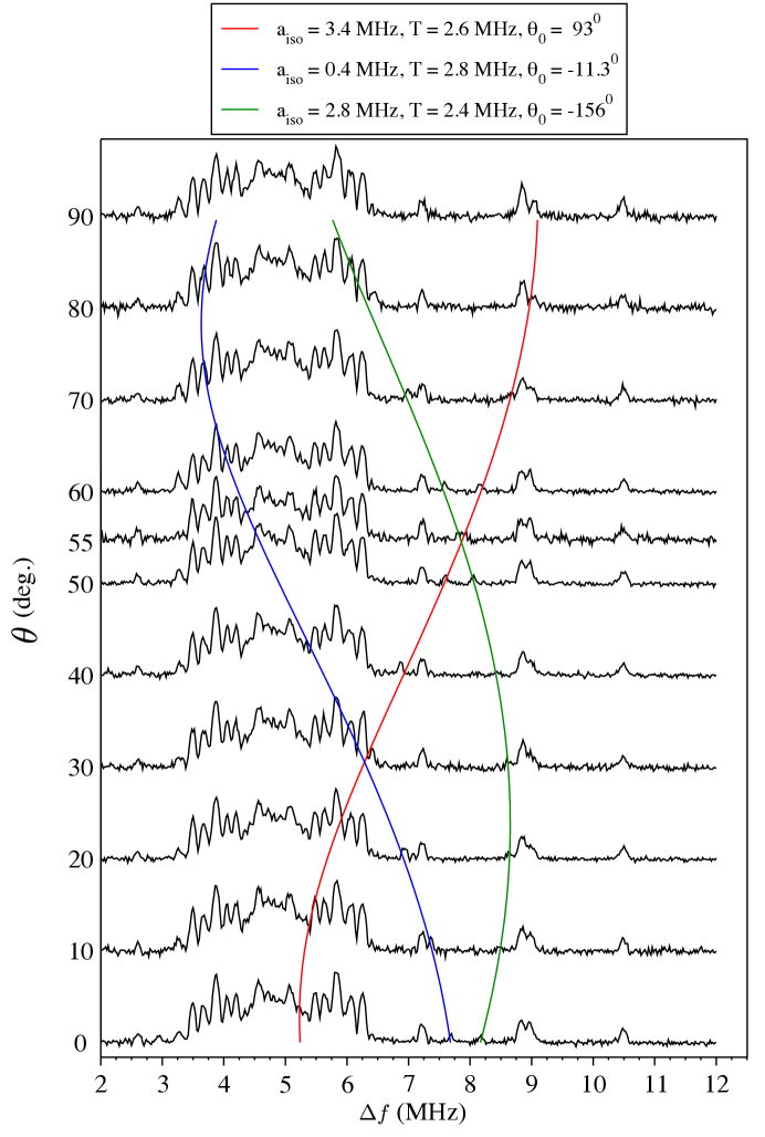
Figure 4.2: Si:Bi ENDOR spectra for the $\left|{11}\right\rangle\to\left|{10}\right\rangle$ ESR transition at 9.75 GHz microwave excitation obtained as a function of $\theta$, where $(\theta-\theta_{0})$ is the angle between the external magnetic field and the $[111]$-direction. The three smooth lines are fits of Equation (4.9), and were used to extract values of the isotropic and anisotropic parts of the hyperfine coupling $a_{\mathrm{iso}}$ and $T$ respectively, as well as the offset angle $\theta_{0}$ which was not known during the experiments.

We now describe the procedure of extracting the three peaks which were found to show $\theta$ dependence. Figure 4.2 shows line 10 spectra obtained for a range of orientation angles between the external field and the $[111]$-direction of the sample crystal. However, the other angle required to fully determine the crystal orientation relative to the magnetic field was unknown in the experiment. Thus, the functional form $\Delta f^{(11)}\left(\theta-\theta_{0},a_{\text{iso}},T\right)$ (Equation (4.9)) was used with free parameters for each peak $a_{\text{iso}}$, $T$ and a constant offset $\theta_{0}$. We managed to fit three curves with this expression to all the spectra as $\theta$ was varied. The peak with $\left(a_{\mathrm{iso}},T\right)\approx\left(3.4,2.6\right)\leavevmode\nobreak\ \mathrm{MHz}$ is consistent with the one previously identified in ESEEM spectra for ESR line 10 [$\left(a_{\mathrm{iso}},T\right)=\left(3.36\pm 0.03,2.56\pm 0.03\right)\leavevmode\nobreak\ \mathrm{MHz}$ (Belli et al., 2011)]. However, this peak is not apparent in Figure 4.1 due to its position and small area at the orientation angle used to perform the measurements in Figure 4.1. The two other couplings were found to have $\left(a_{\mathrm{iso}},T\right)\approx\left(0.4,2.8\right)\leavevmode\nobreak\ \mathrm{MHz}$ and $\left(a_{\mathrm{iso}},T\right)\approx\left(2.8,2.4\right)\leavevmode\nobreak\ \mathrm{MHz}$. It can be seen that for the peaks with non-zero $T$, the difference between theory and experiment can be up to about $0.1$ MHz at low field (see, for example, ESR lines 5 to 2 in Figure 4.1). The deviation is likely due to the experimental uncertainties in the orientation angle $\theta$. In obtaining the rotation spectra in Figure 4.2, the experimental uncertainty in $\theta$ was estimated at $\epsilon_{\theta}\approx\pm 2^{0}$. This leads to a maximum of $\epsilon_{\Delta f}\approx\pm 0.1$ MHz shift in the resonance positions of those peaks for which values of $a_{\mathrm{iso}}$ and $T$ were extracted from the rotation spectra.

4.4 Collapse of Couplings

The magnitude of the polarisation $|P_{i}(\omega_{0})|$ becomes small close to OWPs (Balian et al., 2014) and $df/dB=0$ minima (Mohammady et al., 2010, 2012). Thus, Equation (4.10) tends to the ${}^{29}\text{Si}$ Zeeman frequency $\gamma_{n}B$. This also holds in the anisotropic case (Equation (4.9)). In effect, near these points, the donor might be said to approximately decouple from the bath. For example, for the ESR transition $|12\rangle\to|9\rangle$ $P_{12}(B)=0$ at $B=157.9$ mT and $P_{9}(B)=0$ at $B=210.5$ mT. We note that there is however no $B$-field value where both the upper and lower levels have $|P_{i}(B)=0|$: As we see later, this is not actually essential for complete suppression of spin diffusion. The actual OWP for suppression of decoherence is at $B=188.0$ mT, where $P_{12}=P_{9}$ (Balian et al., 2014). For this transition, the $df/dB=0$ point occurs when

$$P_{12}-P_{9}-\frac{2\delta_{\text{Bi}}}{(1+\delta_{\text{Bi}})}=0.$$ (4.11)

The third term on the left is of order $10^{-4}$ and hence the OWP and frequency-field minimum are very close as discussed earlier.

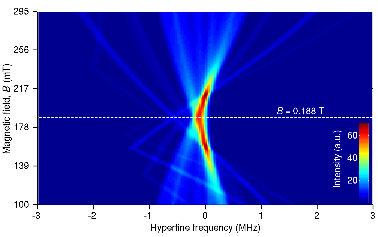
Figure 4.3: Simulated ENDOR as a function of magnetic field $B$, showing collapse of the hyperfine couplings for the $|12\rangle\to|9\rangle$ Si:Bi ESR transition. The OWP is at 0.188 T. Figure adapted from Balian et al. (2012).

4.4.1 Isotropic Case

Figure 4.3 shows a colour map of the qubit-bath hyperfine spectrum for a high density of magnetic fields for the $\left|{12}\right\rangle\to\left|{9}\right\rangle$ Si:Bi ESR line. The spectra were simulated as a function of $B$, using Equation (4.10) and centered about the ²⁹Si nuclear Zeeman frequency. Strikingly, as $B$ approaches the OWP at 0.188 mT, the “comb” of radio frequency hyperfine lines narrows to little more than the width of a single line. This suggests a drastic reduction in the value of the hyperfine couplings, indicating that the bismuth donor has become largely decoupled from the ${}^{29}\text{Si}$ spin bath. Note that as we see in Chapter 5, Chapter 6 and Chapter 7, the enhancement of coherence times involves treatment of the qubit-bath entanglement and the fact that hyperfine couplings are reduced does not fully explain the suppression of decoherence. Nevertheless, this behaviour of collapse in the couplings does provide a spectroscopic signature of OWPs or frequency-field extrema.

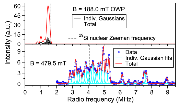
Figure 4.4: Simulated ENDOR at the $B=188.0$ mT OWP (upper panel) and experimental spectrum at 9.755 GHz (lower panel), for the $\left|{12}\right\rangle\to\left|{9}\right\rangle$ Si:Bi ESR transition. Individual Gaussian fits to the data and their sum are also shown in the lower panel. Figure adapted from Balian et al. (2012).

The collapse in the hyperfine couplings is illustrated further in Figure 4.4. The lower panel shows the measured spectrum at 9.755 GHz. Using our experimentally determined hyperfine couplings, the corresponding spectrum at the OWP is shown in the upper panel of Figure 4.4, demonstrating clearly the narrowing of the spectrum [corresponding to the same parameters as Figure 4.3 but at the precise field value of the OWP]. The spectra for a range of magnetic fields is also shown in Figure 4.5, including at the cancellation resonance points. The panels in Figure 4.5 can be thought of as horizontal slices of the high-$B$-density plot in Figure 4.3, rotated to show the intensity on the vertical axis. It can be seen clearly that the most significant suppression of the mostly isotropic couplings occurs near the OWP at $B\simeq 188$ mT.

In constructing the theoretical spectra in Figure 4.3, Figure 4.4 and Figure 4.5, the various areas under Gaussian peaks and the $\text{FWHM}\approx 0.10$ MHz shared by all peaks were extracted from fitting to the $\left|{12}\right\rangle\to\left|{9}\right\rangle$ experimental spectrum. For each coupling, the area of the lower frequency $\left|{12}\right\rangle$ peak was set equal to that of the the higher frequency $\left|{9}\right\rangle$ peak. This was done in order to eliminate to some extent the linear damping in intensity as the radio frequency is lowered in pulsed ENDOR (Schweiger and Jeschke, 2001). Finally, the extracted peak centres were shifted for lower fields according to Equation (4.10).

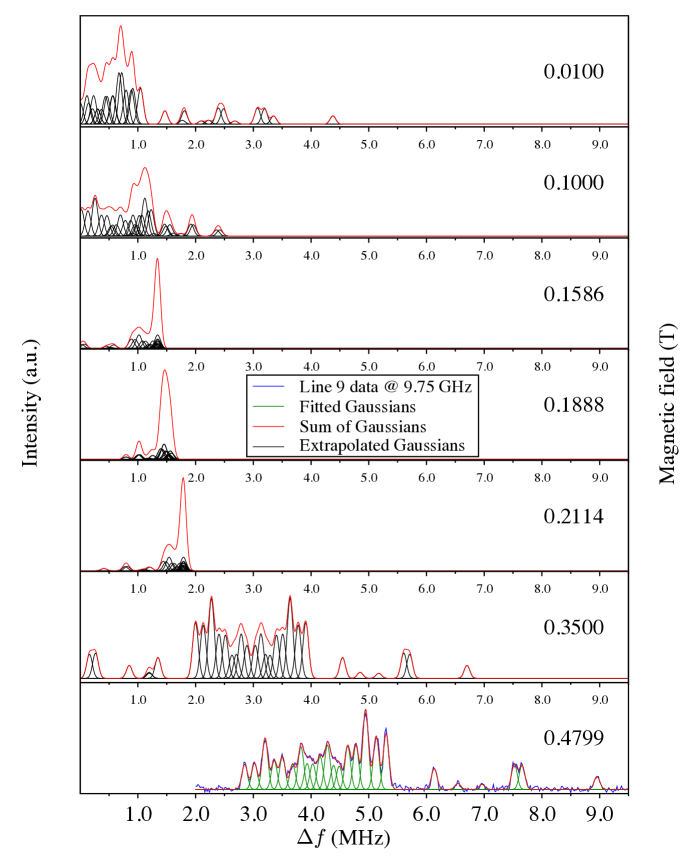
Figure 4.5: Experimental ($B=0.4799$ T, at ESR excitation frequency 9.75 GHz) and extrapolated (simulated) ENDOR spectra for Si:Bi, for the $\left|{12}\right\rangle\to\left|{9}\right\rangle$ ESR transition. Gaussian peaks were fitted to the experimental spectrum. The spectra for $B=0.2114$ T and $B=0.1586$ correspond to the cancellation resonance for levels $\left|{9}\right\rangle$ and $\left|{12}\right\rangle$ respectively. The $B=0.189$ T spectrum is near the OWP. To construct the theoretical spectra, Gaussians peak centres from the experimental spectrum were shifted according to Equation (4.10) as the field $B$ was varied.

It is worth mentioning that near $df/dB=0$ points or OWPs, since $P_{u}\simeq P_{l}$, the ENDOR frequencies for the two ESR levels in the case of isotropic peaks becomes equal (Equation (4.10)), resulting in a single peak in the ENDOR spectrum for each coupling.

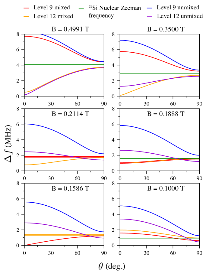
Figure 4.6: Dependence of the $\left(a_{\mathrm{iso}},T\right)=\left(3.36\pm 0.03,2.56\pm 0.03\right)\leavevmode\nobreak\ \mathrm{MHz}$ peak (Belli et al., 2011) on the crystal orientation angle $\theta$ with and without the mixing polarisation terms for the $\left|{12}\right\rangle\to\left|{9}\right\rangle$ ESR transition in Si:Bi. The field $B=0.4799$ T corresponds to 9.75 GHz. Fields $B=0.2114$ T and $B=0.1586$ T are at the cancellation resonance for levels $\left|{9}\right\rangle$ and $\left|{12}\right\rangle$ respectively, and $B=0.1888$ T is near the OWP. The curves were obtained using Equation (4.9) in the case of mixing included. For curves excluding mixing, the polarisation terms were fixed to $\pm$1 at all fields in Equation (4.9).

4.4.2 Anisotropic Case

Figure 4.6 shows the theoretical $\theta$ dependence of the peak with $\left(a_{\text{iso}},T\right)=\left(3.36,2.56\right)$ MHz (Belli et al., 2011) as the field is lowered for the $\left|{12}\right\rangle\to\left|{9}\right\rangle$ transition, for the two cases of allowing $P(B)$ to vary with $B$ (mixing included), and fixing $|P(B)|=1$ (unmixed). This anisotropic peak was identified for the unmixed level $\left|{10}\right\rangle$ (Belli et al., 2011). The results illustrate the significance of the mixing term or polarisation $P(B)$ in causing the suppression of $\theta$ dependence, or equivalently the anisotropic part of the hyperfine coupling at fields close to OWP.

4.5 Conclusion

In conclusion, we presented measurements of the hyperfine couplings between a hybrid qubit (bismuth donor) and a spin bath of ${}^{29}\text{Si}$ impurities which suggest that isotropic couplings dominate. In using pulsed ENDOR as opposed to CW, we demonstrated the feasibility of ²⁹Si nuclei as qubits. The decoherence of ²⁹Si nuclei is the topic of Chapter 8. We further demonstrated the suppression of couplings in both cases of isotropic and anisotropic couplings, serving as a clear signature of OWPs which are discussed in Chapter 5, Chapter 6 and Chapter 7. Our results motivate both spectroscopic and decoherence measurements for the Si:Bi system in the excitation frequency range $5-7.5$ GHz for ESR-type OWPs and around 1 GHz for NMR-type ones (Figure 3.3).

We note that by using much higher-resolution CW ENDOR and by performing experiments which adequately sample all crystal directions, it is possible to map hyperfine couplings to shells of ²⁹Si with known positions from the donor site, as was achieved for the Si:P system in Hale and Mieher (1969a) and Hale and Mieher (1969b). However, this requires considerable experimental effort; also, as we shall see in later chapters, hyperfine couplings calculated using effective mass theory (Section 2.4.3) suffice to give coherence decays in excellent agreement with experiment. Nevertheless, the order of magnitude and range of measured couplings agree with the calculated values, and this give us confidence in using the model described in Section 2.4.3 for our decoherence studies of the hybrid qubit. Later in Chapter 8, for decoherence of ²⁹Si nuclear impurities, we propose a model which relies heavily on symmetries of the electronic wavefunction, and thus would benefit much more from experimental ‘$J\to{\bf r}_{n}$’ mapping offered by CW studies.

5  |  Coherence Times of
Hybrid Qubit

This chapter concerns the decoherence dynamics of the hybrid qubit. We investigate the decoherence mechanism and calculate coherence times using the CCE for the Hahn spin echo and single-spin FID. We also compare our results to experimental coherence measurements. Although the Hahn spin echo is the lowest order CPMG dynamical decoupling sequence, it is often the case that the shortest measured $T_{2}$ times for solid-state systems are reported for this sequence (in order to remove static magnetic field inhomogeneities as discussed in Section 2.2.2). Therefore, we discuss the Hahn echo in the current chapter, and present higher-order dynamical decoupling sequences (CPMG$N$, $N>1$) in the next chapter.

We begin by describing our numerical method of calculating coherence times of the hybrid qubit. We then present calculated coherence times for the hybrid qubit at the forbidden transitions for which fast quantum control was demonstrated as discussed in Chapter 3. These were the first CCE calculations taking into account full quantum state-mixing of the central system for decoherence in a spin bath. The calculations were performed and published in Morley et al. (2013) by S.J.B. with supervision from Dr. Wayne Witzel at Sandia National Laboratories, USA. Prior to these results, only weak state-mixing was investigated for Si:Bi in the unmixed regime by varying an effective gyromagnetic ratio ($\equiv df/dB$) as a function of $B$ (George et al., 2010). This treatment limited access to forbidden transitions. Also, as we shall see below and found in Balian et al. (2014) which partly studies for differences between spin bath and classical noise decoherence, effective gyromagnetic ratio (or equivalently $df/dB$ (Vion et al., 2002)) treatments do not reliable describe decoherence of the hybrid qubit in all regimes.

In Chapter 3, OWPs were introduced as field values corresponding to suppression of decoherence in spin baths. Here, we present the first validation of OWPs as sweet-spots, first published in Balian et al. (2012). We proceed to numerically calculate coherence times across orders of magnitude variation as a function of magnetic field $B$, and find excellent agreement with experiment in nearly all field regimes (published in Balian et al. (2014)).

For the Hahn spin echo near OWPs, we find that in order to simulate coherence times, one must consider clusters of three interacting spins within the many-body quantum bath, since independent pairs do not even give finite $T_{2}$ decay times; i.e. OWPs almost completely suppress decoherence driven by pair correlations. In all regimes except for OWP regions for the Hahn spin echo and moderate CPMG (as we shall see in Chapter 7), the usual independent pairs of flip-flopping spins dominate. This finding formed the first part of our work published in Balian et al. (2015); the other part concerns $N>1$ dynamical decoupling and is the topic of Chapter 7.

5.1 Fitting Coherence Decays

Before presenting coherence calculations and measurements it is important to briefly discuss how $T_{2}$ times are extracted from coherence decays. For high temperatures ($\gtrsim 14$ K), coherence decays for donors in silicon are exponential and limited by the spin-lattice relaxation $T_{1}$. For the lower, cryogenic, temperatures we consider the coherence times are temperature independent and are well-fitted to a combination of exponential and stretched exponential time decays:

$$S=\exp{\left(-\frac{t}{T^{\prime}_{2}}-\left[\frac{t}{T_{2}}\right]^{n}\right).}$$ (5.1)

For the Hahn spin echo case, $t=2\tau$, where $\tau$ is the time either side of the refocusing pulse. The stretched exponential part with time constant $T_{2}$ in Equation (5.1) characterises nuclear spin diffusion, and for this process, the exponent $n$ is known to be about 2 (Witzel et al., 2005), thus resulting in a near-Gaussian decay in coherence. In Equation (5.1), all other decoherence mechanisms, including those arising from donor-donor interactions from measurements on an ensemble of donors, are characterised by $T^{\prime}_{2}$. Clearly, the shortest decoherence time is the limiting one. Note that for a decay of form $\exp{[-(t/T_{2})^{n}]}$, $T_{2}$ is the time taken for the coherence to drop to $1/e$ of its initial value and this holds $\forall\ n$.

5.2 Numerical Method:
CCE with Central State Mixing

The CCE method was described in detail in Section 2.5. It is a well-established method for accurately calculating the coherence decay $\mathcal{L}(t)$ of a central spin system in a quantum spin bath (Yang and Liu, 2008a, b, 2009). The code for our implementation of the CCE is open-source and free to use under the GNU licence (see Appendix A for details and how to cite). Here, we describe the method used to calculated coherence decays of the hybrid qubit in a bath of ²⁹Si impurities, using our implementation of the CCE. We also present results which we use to establish numerical convergence of the coherence decays with respect to heuristic cluster cut-offs.

The CCE was applied for nuclear spin diffusion in a dipolar ²⁹Si bath coupled to the qubit via the hyperfine interaction as described in Chapter 2. Importantly, the central spin Hamiltonian did not include a bare electron with an effective gyromagnetic ratio taking account of mixing as in previous studies (George et al., 2010). Instead, we used the full donor Hamiltonian Equation (3.1) in Chapter 3, including electron-nuclear mixing. We did not include phonon-induced relaxation effects in our simulations, as temperatures were cold enough such that $T_{1}\gg T_{2}$. Also, the donor concentration was much less than that of the ²⁹Si nuclei and hence donor-donor decoherence was expected to be on much longer timescales and hence neglected in our studies.

5.2.1 Initial State

For our simulations, crystal sites of a cubic silicon superlattice (see Appendix C for details) were uniformly populated with ²⁹Si nuclei ($I=1/2$) with the natural fractional abundance of 0.0467 and with equal probability of spin-up ($\left|{\uparrow}\right\rangle$) and spin-down ($\left|{\downarrow}\right\rangle$) forming the pure product initial bath state. The size of the superlattice giving convergent coherence decays was established as we describe below.

We assumed that the bath is not initially entangled with the bismuth donor. The bismuth donor was then put into an equal superposition of the two eigenstates being excited: $\left|{\psi(t_{0})}\right\rangle=\tfrac{1}{\sqrt{2}}\left(\left|{u}\right\rangle+\left|{l}\right\rangle\right)\otimes\left|{\mathcal{B}(t_{0})}\right\rangle$.

5.2.2 Dynamics

For the closed dynamics of each reduced problem (i.e. for the bismuth donor and cluster of bath spins), the total Hamiltonian comprised of nuclear Zeeman and dipolar intra-bath interaction terms given in Equation (2.19) (assuming a secular dipolar interaction (Section 2.4.2)), as well as the isotropic hyperfine interaction in Equation (2.21). Such reduced problem Hamiltonians were decomposed to obtain the free evolution operators $\hat{U}(\tau)$.

Note that in the CCE method, the pure dephasing approximation is not required, and the interaction Hamiltonian in general includes terms which depolarise the states of the central system. Our CCE calculations include the $\hat{S}^{-}\hat{I}^{+}+\hat{S}^{+}\hat{I}^{-}$ terms in the hyperfine interaction Hamiltonian Equation (2.21), but we find that these give small corrections to the case when only $\hat{S}^{z}\hat{I}^{z}$ terms are included. This was expected due to the large mismatch between electronic and nuclear gyromagnetic ratios.

The mixed Zeeman basis of the hybrid qubit was employed as described in Chapter 3. To save computational time, we note that in our implementation, the full 20-dimensional basis was truncated to exclude matrix elements which remain uninvolved in the dynamics for all times. This is because the donor Hamiltonian is in block diagonal form (of at most $2\times 2$ matrices) and only those Zeeman basis states required to fully represent the two energy levels for the transitions are involved in the dynamics. We note however for levels forming doublets, even for the simple Ising-only hyperfine interaction involving only $\hat{S}^{z}$-coupling, since $\left\langle{\pm,m}\right|\hat{S}^{z}\left|{\mp,m}\right\rangle\neq 0$, the Zeeman states for the level with which the transition level forms a doublet are also required. For example, if one of the levels in the transition is $\left|{+,m}\right\rangle$, then the four Zeeman states $\left|{\pm 1/2,m\mp 1/2}\right\rangle,\left|{\mp 1/2,m\pm 1/2}\right\rangle$ are in general needed. Note that for transitions between doublets adjacent in $m$ (and assuming an Ising-only interaction to the bath), four Zeeman states in total are required.

When including the non-Ising terms in the hyperfine interaction, the 20 basis states are strictly required. However, our numerical results show that (i) the effect of the non-Ising term is negligible as mentioned above, and (ii) even if the non-Ising term is included with the truncated basis above, the results are indistinguishable from the case of including the full 20-dimensional basis with non-Ising terms. The latter is indicative of the weakening perturbative effect of the non-Ising terms as an increasing number of spin flips are required to navigate into states far in $m$ from those involved in the transition.

To calculate the electron-bath hyperfine couplings, we use the Kohn-Luttinger electronic wavefunction for the bismuth donor in silicon with an ionization energy of 0.069 eV as described in Section 2.4.3. Calculated qubit-bath couplings were of the same order as those obtained from the data in Chapter 4. The experimental data presented in Chapter 4 suggested that isotropic couplings to the bath dominate; hence anisotropic couplings were neglected and the simulations were largely insensitive to orientation (apart from the orientation dependence in the intra-bath dipolar interaction).

In obtaining the ²⁹Si–²⁹Si dipolar terms it was assumed that the external magnetic field was large enough to conserve the total ²⁹Si Zeeman energy, hence assuming the secular dipolar approximation. The strength of the dipolar interaction was calculated as shown in Section 2.4.2, with the magnetic field direction chosen to match that in experiments with which we compare our calculated decays.

As for dynamical decoupling control (including the 1-pulse Hahn echo), we assumed negligible duration of the $\pi$-pulse compared to the total evolution time and applied instantaneous spin-flip pulse(s). We note that for a spin system with more than a pair of energy eigenstates, the non-resonant states (i.e. $\left|{i\neq u,l}\right\rangle$) must remain unchanged when applying refocusing pulses. Therefore, the $\pi$-pulse operator was taken as $(\left|{u}\right\rangle\left\langle{l}\right|+\left|{l}\right\rangle\left\langle{u}\right|+\sum_{n\neq u,l}\left|{n}\right\rangle\left\langle{n}\right|)\otimes\hat{\mathds{1}}_{\mathcal{B}}$, in which the sum includes the other non-resonant eigenstates which can be formed in the Zeeman representation of $\left|{u}\right\rangle$ and $\left|{l}\right\rangle$.

Finally, the final state is written as a density matrix and the partial trace over the bath computed to recover the reduced density matrix of the central system. The orthonormal basis used to perform the trace operation is formed of all possible product states of the cluster bath. The off-diagonal of the reduced density matrix corresponds to the coherence as described in Chapter 1 and Chapter 2. The resulting reducible coherences are then used in the CCE formalism as described in Section 2.5.

5.2.3 Cluster Heuristics and CCE Convergence

The total size of the spin bath is dictated by the spatial extent of the wavefunction which decays exponentially with distance from the donor site, and a superlattice of side length 160 Å (with $10^{4}$ impurities) gives convergent coherence decays. Figure 5.1 shows convergence of the CCE as we increase the lattice space diagonal. The donor was situated at the centre of a cubic superlattice of side length that was varied from 30 Å to 182 Å. Including spins outside the 160 Å cube had minor effect on the coherence decays.

Due to cubic decay of the dipolar interaction as the distance between a pair of ²⁹Si spins is increased, it is not necessary to include all spin clusters in the calculation. At the lowest non-trivial CCE order (CCE2), spins separated by at most the 4-th nearest neighbor distance in silicon ($\sqrt{11}a_{0}/4$, where $a_{0}=5.43$ Å) are enough to give convergent decays (provided the CCE converges at the two-cluster level with respect to cluster size). Convergence in the separation cut-off as it is increased from the nearest neighbour to the 3rd nearest neighbour distance are shown in Figure 5.2.

To choose three-clusters (i.e. including clusters of three bath spins), we loop over all sites in the crystal and add to each two-cluster only those spins that are at most separated by $\sqrt{11}a_{0}/4$ from any of the two spins in the two-cluster. The same procedure was applied to choose higher-order clusters, by adding spins to clusters one order down. The numbers of 2, 3, 4, and 5-clusters found with these heuristic cut-offs are each of order $\approx 10^{4}$. The total computational time taken to diagonalise all these reduced problems is at most about a day on a desktop machine for a single initial bath state, with the most intensive (CCE5) of our calculations.

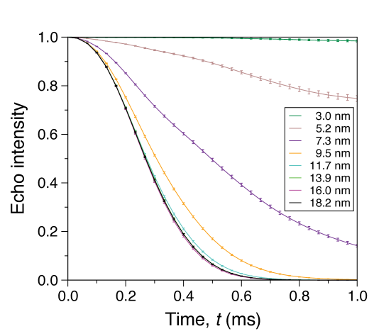
Figure 5.1: Convergence of the two-cluster correlation expansion for spin echo decays in Si:Bi at 4 GHz with respect to the superlattice size. Pairs of ²⁹Si nuclei with separations up to the 3rd nearest neighbour distance in the silicon lattice were included in the calculation. The error bars are the standard deviation of the mean intensity after 100 random spatial and initial state configurations of ²⁹Si nuclei, and the external magnetic field was chosen to be $B=0.3446$ T so the $\left|{11}\right\rangle\to\left|{10}\right\rangle$ Si:Bi transition was excited. Figure adapted from Morley et al. (2013).

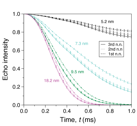
Figure 5.2: Convergence of the two-cluster correlation expansion for spin echo decays in Si:Bi at 4 GHz with respect to the pair-separation cut-off. The maximum distance between paired ²⁹Si nuclei is increased by pairing 1st, 2nd and 3rd nearest neighbours. Convergence is achieved for the 3rd nearest neighbors. The 1st, 2nd and 3rd nearest neighbour separations in the silicon lattice are $\tfrac{\sqrt{3}}{4}a_{0}$, $\tfrac{\sqrt{2}}{2}a_{0}$, and $\tfrac{\sqrt{11}}{4}a_{0}$ respectively, with $a_{0}=5.43$ Å. The results are compared for a range of lattice sizes. The error bars are the standard deviation of the mean intensity after 100 random spatial and initial state configurations of ²⁹Si nuclei, and the external magnetic field was chosen to be $B=0.3446$ T so the $\left|{11}\right\rangle\to\left|{10}\right\rangle$ Si:Bi transition was excited. Figure adapted from Morley et al. (2013).

5.2.4 Initial State Averaging

Finally, in order to simulate multiple experimental runs on the same spatial bath configuration (time-average), the coherence calculated for each reduced problem can be solved for all the non-interacting bath eigenstates in the cluster and the results averaged. This effect can also be simulated by applying the CCE to different random configurations of initial bath state (i.e. random sampling from the thermal ensemble) and obtaining the mean over these results. However, this method takes longer computational time. Also, for measurements on an ensemble of qubits, the results should be averaged over different spatial as well as initial state configurations of the bath. However, we note that the differences in coherence between the different averages are not significant for the large spin baths we consider.

Note that all these averages are over the complex coherence (coherent averaging); the real and imaginary parts of the coherence correspond to orthogonal axes of the in-plane magnetisation. The modulus of the coherence should strictly only be taken at the end of the calculation. Nevertheless, applying the modulus to coherences before averaging (incoherent averaging) does not significantly affect the decays.

Before discussing coherence times near OWPs, we begin by presenting our simulations of $T_{2}$ for the hybrid qubit at $S$-band frequencies, where fast quantum control was experimentally demonstrated in Chapter 3.

5.3 Coherence Times at Forbidden Transitions

In this section, we present calculated coherence times of the hybrid qubit in natural silicon at $S$-band ESR excitation frequency ($f\approx 4$ GHz) where fast Rabi oscillations were demonstrated as described in Chapter 3 for the forbidden transition of Si:Bi.

Importantly, our CCE calculations enabled us to attribute the dominant decoherence mechanism for the hybrid qubit at $S$-band to nuclear spin diffusion from the spin bath of ²⁹Si nuclear impurities. We compare our simulations with experimental data and establish a coherence time which can be up to five orders of magnitude longer than the qubit manipulation time in this regime.

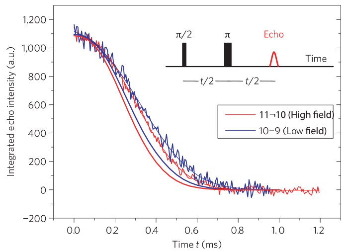
Figure 5.3: Example spin-echo coherence decays measured for both Si:Bi transitions at 4 GHz, with a temperature of 10 K. The echo coherence decay is limited by ²⁹Si nuclear spins, as parameterized by $T_{2}$ in the fitting function $\exp{(-t/T^{\prime}_{2}-t^{n}/T_{2}^{n})}$, where $T^{\prime}_{2}$ is the spin coherence time expected after isotopic enrichment. The exponent $n$ was used as a fitting parameter. The smooth thin lines are these fits whereas the smooth thick lines show a simulation with no free parameters using the cluster correlation expansion. This shows that ²⁹Si impurities dominate the spin decoherence. The thickness of the line is of the order of the standard deviation of the mean intensities after 100 random spatial configurations of ²⁹Si nuclei. As discussed in Chapter 2, the refocusing $\pi$-pulse removes static magnetic field noise from ²⁹Si couplings to the qubit. The magnetic field direction was perpendicular to the $[111]$ crystal direction. Figure adapted from Morley et al. (2013).

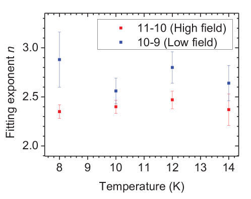
Figure 5.4: Dependence of the fitting exponent $n$ on temperature, showing the expected range of $n\approx 2$ expected for nuclear spin diffusion. Figure adapted from Morley et al. (2013).

5.3.1 Numerical Results

The calculated decays are shown in Figure 5.3 as solid lines. We fitted the decays with the same function as used for fitting to the experimental data (Equation (5.1)), and an effectively infinite $T^{\prime}_{2}$ (over 1018 s) was obtained, indicating the lack of an exponential component (this was expected as donor-donor processes were ignored in our calculations). The values for the exponent $n$ were obtained as 2.25 for the $\left|{10}\right\rangle\to\left|{9}\right\rangle$ transition and 2.28 for the $\left|{11}\right\rangle\to\left|{10}\right\rangle$ transition with standard errors on the fits of $\pm 0.01$; the values of the exponent are in agreement with those obtained for nuclear spin diffusion in previous studies (Witzel et al., 2005). As for the $T_{2}$ values, these were $0.314\pm 0.0005$ ms for $\left|{11}\right\rangle\to\left|{10}\right\rangle$ and $0.340\pm 0.0007$ ms for $\left|{10}\right\rangle\to\left|{9}\right\rangle$(using the standard errors on the fits). The value of $T_{2}$ for the $\left|{11}\right\rangle\to\left|{10}\right\rangle$ transition is slightly shorter than for the $\left|{10}\right\rangle\to\left|{9}\right\rangle$ and we attribute this trend to the smaller gradient $df/dB$ for the $\left|{10}\right\rangle\to\left|{9}\right\rangle$ transition.

5.3.2 Comparison with Experiment

Our CCE decays are shown in Figure 5.3 and compared to experimental Hahn spin echo decays at $S$-band. The CCE simulations had no free parameters extracted from the experiment, thus demonstrating that ²⁹Si impurities dominate the spin echo decay at low temperatures. Values for the exponent from fits to experimental data are shown in Figure 5.4 and are in agreement with the expected nuclear spin diffusion $n$ of near-Gaussian ($n\simeq 2$). The small discrepancies between theory and experiment are expected to be mainly due to ignoring possibly undiscovered sources of decoherence in the simulation and limited knowledge of the donor electron wavefunction. The experimental coherence times also show the expected trend due to $df/dB$.

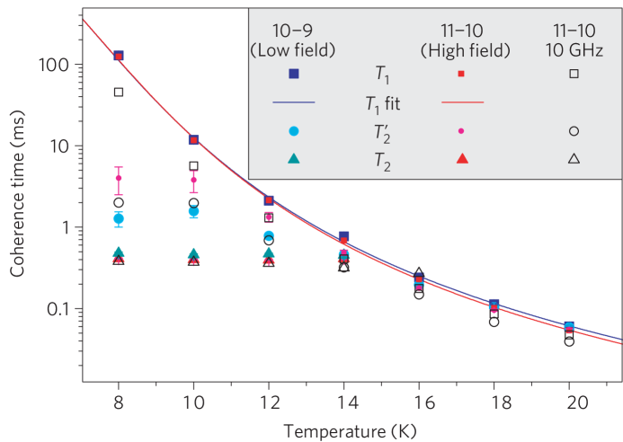
Figure 5.5: Coherence times of hybrid electron-nuclear qubits as a function of temperature for both resonances at 4 GHz with previously published data at 10 GHz (Morley et al., 2010) for comparison. The 4 GHz spin-lattice relaxation rates are $1/T_{1}$. The error bars show the standard errors, which are in many cases smaller than the symbol. Figure adapted from Morley et al. (2013).

5.3.3 Discussion

Measured coherence times in natural silicon, including those extracted from the experimental decay curves in Figure 5.3, are shown in Figure 5.5 as a function of temperature. It can be seen that $T_{2}$ can reach 0.4 ms, in good agreement with the predicted theoretical values above, while $T^{\prime}_{2}$ can be about 4 ms. There are no OWPs in this region for the hybrid qubit, and hence no significant enhancement of $T_{2}$. Therefore, the best strategy possible is to use isotopic enrichment to reach the 4 ms coherence time.

It is important to note that if the hybrid qubit was approximated as a simple spin-1/2 with an effective field-dependent gyromagnetic ratio as in George et al. (2010), it would not be possible to obtain coherence decays for the forbidden transition $\left|{10}\right\rangle\to\left|{9}\right\rangle$.

The $S$-band coherence measurements were performed by Dr. Petra Lueders, Dr. Gavin Morley and Dr. Hamed Mohammady at ETH Zurich.

5.4 Coherence Times at Optimal Working Points

As introduced in Chapter 1, the OWPs of the hybrid qubit we consider are those near where there is suppression of decoherence from spin bath environments. OWPs can be understood by considering the qubit-bath entanglement and the back-action of the qubit on the environment.

5.4.1 Loss of Which-Way Information

OWPs correspond to $B$-field values where the unitaries associated with the upper and lower central qubit states equalise: $\hat{T}_{l}\simeq\hat{T}_{u}$, occurring when $P_{u}\simeq P_{l}$ as found in Balian et al. (2014). This means that the combined qubit-bath state after evolution following a $\pi/2$-pulse (Equation (2.17)) can now be written as

$$\left|{\psi(t)}\right\rangle=\frac{1}{\sqrt{2}}\left(e^{-iE_{u}t}\left|{u}\right\rangle+e^{-iE_{l}t}\left|{l}\right\rangle\right)\otimes\hat{T}_{u}(t)\left|{\mathcal{B}(0)}\right\rangle,$$ (5.2)

with the product form preserved (assuming pure dephasing). Crucially, the state is no longer entangled and the ‘which-way’ information in the environment or the back-action of the central qubit on the environment is minimal. Therefore, entanglement-induced (quantum bath) decoherence is suppressed:

$$|\mathcal{L}(t)|=|\langle\mathcal{B}(0)|\hat{T}_{u}^{\dagger}(t)\hat{T}_{u}(t)|\mathcal{B}(0)\rangle|=|\langle\mathcal{B}(0)|\hat{\mathds{1}}|\mathcal{B}(0)\rangle|=1.$$ (5.3)

In practical realisations, OWPs have become closely associated with field values where the frequency-field gradient $df/dB=0$ (Wolfowicz et al., 2013) or ‘clock transitions’. However, for donor spin systems, the OWP is close to but not exactly at the $df/dB=0$ point, and not all $df/dB=0$ points are OWPs as shown in Balian et al. (2014). In the latter, it was also shown that it is not possible to fit functional forms of $df/dB$ to describe the coherence $T_{2}(B)$ for all $B$.

Figure 5.6: Suppression of spin bath decoherence near OWPs of the hybrid qubit in a nuclear spin bath (^natSi:Bi). Figure was adapted from Balian et al. (2014). Each dot represents the $T_{2}$ extracted from coherence decays obtained using the cluster correlation expansion (CCE). The coherence times are the Hahn spin echo $T_{2}$, and near the OWPs, these were extracted from the short-time behaviour of CCE2 decays, since pair correlations are strongly suppressed on the actual timescale of $T_{2}$ near OWPs. Such short-time $T_{2}$ times are in agreement with those obtained from full decays of the converged CCE3 near OWPs established in Balian et al. (2015) (see Section 5.4.3 for details).

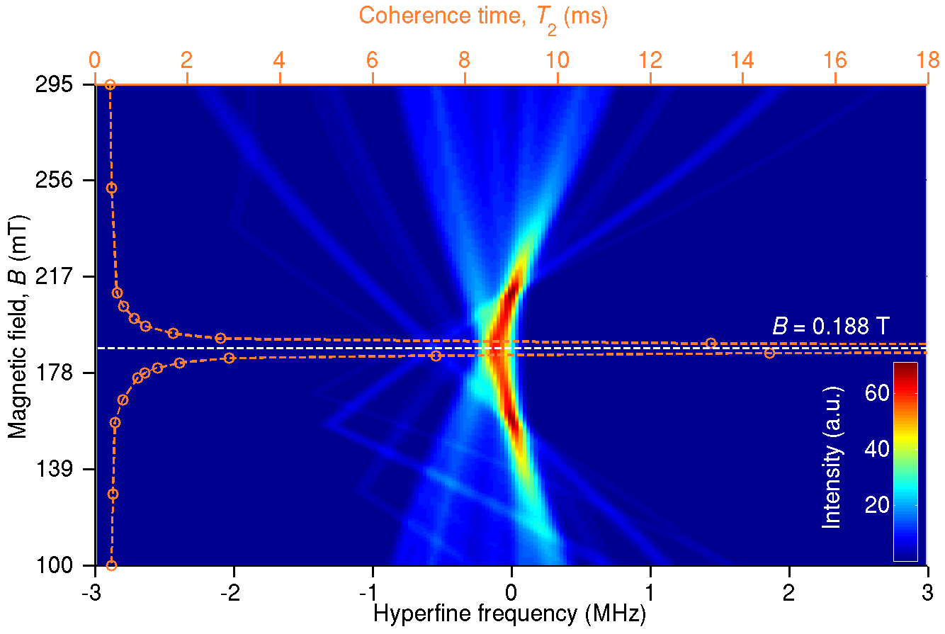
Figure 5.7: Suppression of Bi-${}^{29}\text{Si}$ spin bath decoherence for the $|12\rangle\to|9\rangle$ ESR transition. Simulated ENDOR and nuclear spin diffusion coherence times $T_{2}$ (Hahn echo) as a function of magnetic field $B$, showing collapse of the hyperfine couplings and a sharp increase in $T_{2}$ as the field approaches the $B=188.0$ mT optimal working point (OWP). The dashed line is a fit. Figure adapted from Balian et al. (2012). Coherence times in the OWP region were extracted from the short-time behaviour of CCE2 (Details are given in Section 5.4.3).

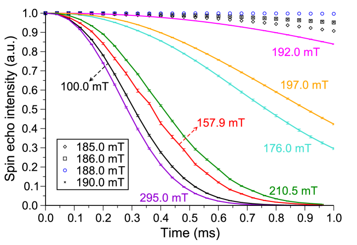
Figure 5.8: Calculated donor Hahn spin echo decays from which coherence times in Figure 5.7 were extracted. Figure adapted from Balian et al. (2012). Decays are for CCE2 (Hahn echo), shown here for short times. For converged decays near the OWP see Section 5.4.3.

5.4.2 Suppression of Nuclear Spin Diffusion

In this section, we present numerical CCE calculations showing enhancement of the spin diffusion coherence time $T_{2}$ at an OWP (Balian et al., 2012, 2014). The orders of magnitude enhancement for coherence times at two OWPs of the hybrid qubit is illustrated in Figure 5.6.

The CCE simulations were performed for the $\left|{12}\right\rangle\to\left|{9}\right\rangle$ and $\left|{12}\right\rangle\to\left|{11}\right\rangle$ Si:Bi transitions. Once again, low temperatures were assumed and hence phonon-induced relaxation effects ignored. We also assumed that the donor concentration was low such that the decoherence was dominated by nuclear spin diffusion from the ²⁹Si spin-1/2 bath and not by donor-donor processes.

Figure 5.7 which shows the behaviour around the $B=188.0$ mT OWP associated with the $|12\rangle\to|9\rangle$ transition, superposed on the colour map of the qubit-bath hyperfine spectrum (Figure 4.3). The behaviour of $T_{2}$ was striking and unexpected: The coherence time predicted by CCE simulations increases asymptotically at the OWP. Away from the OWP, the results agree well with experimentally measured values of approximately 0.7 ms (George et al., 2010). In George et al. (2010), in a regime of weak state-mixing, simulations using an effective gyromagnetic ratio indicated that $T_{2}$ was slightly reduced (by about 5%) in a regime corresponding far from the OWP (but with some weak $df/dB$ variation). These results, on the other hand (which in contrast to George et al. (2010) employed a full treatment of the quantum eigenstate mixing) show rather an effect very sharply peaked about the OWP: Nuclear spin diffusion is predicted to be largely suppressed, but over an extremely narrow magnetic field range.

Figure 5.8 shows a sample of CCE spin echo decays from which the $T_{2}$ times in Figure 5.7 were extracted, and also serves to further illustrate the sharp increase in $T_{2}$. Similar suppression is present for other OWPs in Si:Bi. OWPs are also expected to lead to suppression of decoherence arising from the interaction with a bath of donors (Mohammady et al., 2010).

The calculated coherence decays in Figure 5.7 and Figure 5.8 are the average over 100 initial spatial configurations of ²⁹Si.

5.4.3 Many-Body Correlations

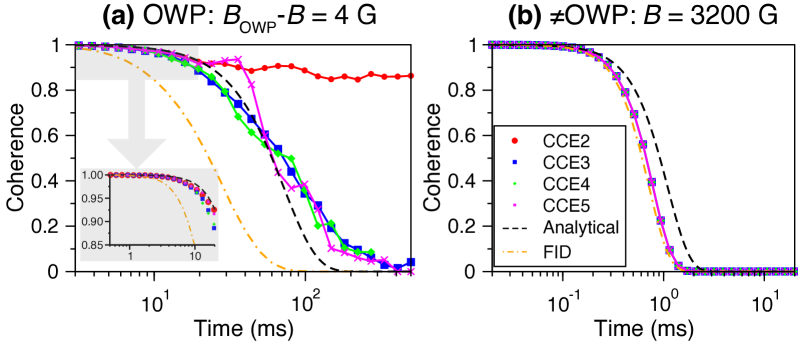
Figure 5.9: Shows quantum many-body calculations of the Hahn spin echo using the cluster correlation expansion (CCE) method. (a) Near OWPs, calculations using a bath of independent spin pairs only (red, CCE2) do not even predict a finite decay time but, surprisingly, calculations with clusters of three spins (blue, CCE3) are already well-converged. The dashed lines used a closed-form equation derived from the short time behaviour, found in Balian et al. (2014) to yield good agreement with experiments; this indicates that three-cluster results too give good agreement with measurements. The formula is discussed in Chapter 6. Higher order CCE can encounter numerical divergences (which can be attenuated by ensemble averaging); this accounts for the discrepancies with CCE5. (b) Far from the OWP, independent pairs (CCE2) already give results in good agreement with CCE3-5 as well as experiments. The single-spin free induction decay (FID) is also shown for comparison. Note that the analytical formula approximates the decay by a pure Gaussian. CCE calculations were performed for a bismuth donor in natural silicon for $B$ along $[100]$ and the $\left|{14}\right\rangle\to\left|{7}\right\rangle$ transition for which $B_{\text{OWP}}=799$ G. In (a), $B=795$ G while for (b), $B=3200$ G. Figure adapted from Balian et al. (2015).

In the high-field regime of the hybrid qubit where the state-mixing is weak, CCE2 or the pair-correlation approximation is a good approximation to the coherence when considering only dipolar interactions in the bath affecting the spin echo, as these are at most a few kHz and hence perturbative compared to the hyperfine interactions in the MHz range involving the donor electron. Experimental Hahn echo decays are well predicted by CCE2 in these regimes or for simple spin-1/2 qubits without OWPs (Witzel and Das Sarma, 2006). However, this argument does not hold in regions close to an OWP as seen in Chapter 4 where the collapse of hyperfine couplings to the bath was demonstrated. In the vicinity of the OWPs (where $P_{u}\simeq P_{l}$), the CCE2 Hahn echo decay fails to converge at all times and no decays can be obtained other than initially, for a short time.

We find that to simulate recently measured Hahn echo decays at OWPs (lowest-order dynamical decoupling), one must consider clusters of three interacting spins, since independent pairs of bath spins (pair correlations) do not even give finite $T_{2}$ decay times. The CCE2 Hahn echo results (for all $t$) are at odds with experiment since they predict infinite coherence times (Balian et al., 2014). As mentioned above, coherences decay initially, then after a short time, the decays stop.

In order to clarify the origin of the measured coherence decays, we employ quantum many-body simulations of the system-bath dynamics using the CCE including contributions from clusters of up to 5 spins (CCE5). The CCE$3-5$ many-body calculations we undertake are significantly more computationally challenging than CCE2 or pair correlation calculations. The converged numerical results are presented in Figure 5.9 both near and far an OWP of Si:Bi for the Hahn spin echo, the latter denoted ‘$\neq$OWP’. We show that including three-spin clusters (CCE3) gives converged results while qubit-bath correlations from only spin pairs (CCE2) give little decay (red line) except at short timescales. The three-spin clusters suffice to give decays in good agreement with experimental results (Wolfowicz et al., 2013). Importantly, it can also be seen that all orders have similar short time behaviour and that the inclusion of the three-clusters in effect recovers the short time behaviour of the pair decays. Hence, the short time behaviour of the pair correlation decay is sufficient to establish an order-of-magnitude estimate of $T_{2}$.

It is worth clarifying the physical meaning of the above-mentioned three-cluster result. It is not a matter of enlarging the quantum bath with additional nuclear spin clusters of the same size. As illustrated in Figure 2.5, a three-spin cluster (blue) can be decomposed into three distinct flip-flopping pairs (each nuclear spin can contribute to more than one flip-flopping pair). Put simply, if all such three-clusters in a given, randomly generated set of impurities in a crystal are decomposed into the constituent flip-flopping pairs, an infinite decay time is obtained. If, however, the exact same configuration of spin impurities are aggregated into the ‘triangle’ structures illustrated in Figure 2.5, the correct experimental behaviour emerges. To our knowledge, there is no other example of a central spin system which so fully eliminates the pair-driven dynamics.

5.4.4 Comparison with Experiments

We compare our CCE simulations (short-time CCE2 Hahn echo) with experiment across a broad range of magnetic fields and transitions in Figure 5.10; for ESR-type transitions in the high-field and OWP regions (filled symbols) and NMR-type transition (empty symbols) where $T_{2}$ varies by orders of magnitude. The measured values are in excellent agreement with the CCE calculations.

Measurements were made at 4.8 K using ESR with a microwave frequency of 9.77 or 7.03 GHz (filled symbols), or electron-nuclear double resonance (ENDOR) between 200 MHz and 1 GHz using the method described in Morton et al. (2008) (empty symbols), at magnetic fields between 100 and 450 mT. The experiments were performed by Dr. Gary Wolfowicz at UCL under supervision from Professor John Morton.

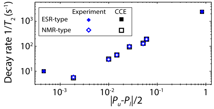
Figure 5.10: Comparison between theoretically predicted and measured $T_{2}$ in ^natSi:Bi for various transitions, showing remarkable agreement across a wide range of mixing regimes – magnetic fields and transitions quantified by $|P_{u}-P_{l}|$. The Bi donor concentration was $\leq 10^{16}$ cm^-3, and decoherence times are limited by ²⁹Si spin diffusion. Figure adapted from Balian et al. (2014).

As shown in Figure 5.6, $T_{2}$ varies sharply with magnetic field over a small region of $B$; especially for ESR-type OWPs (corresponding to an order of magnitude over a few G). Therefore, for direct quantitative comparisons between the calculations and experimental ensemble measurements, inhomogeneous broadening due to ²⁹Si, which has full width at half maximum (FWHM) of about 4 G in natural silicon, might also have to be considered. This effect is not only important for predicting the rate of experimental decays but also their shape. The broadening can be simulated by convolving the calculated decays $\mathcal{L}_{B}(t)$ with a Gaussian magnetic field distribution with standard deviation $w\simeq 2$ G:

$$D_{B}(t)=\frac{1}{w\sqrt{2\pi}}\int{e^{\frac{-\left(B-B^{\prime}\right)^{2}}{2w^{2}}}\mathcal{L}_{B}(t)dB^{\prime}}.$$ (5.4)

The ESR-type OWP point in Figure 5.10 (the first data point where $P_{u}$ is closest to $P_{l}$), is the result of the convolution (with $B=B_{\text{OWP}}$) shown in Figure 5.11, in good agreement with experiment. The long-time discrepancy is probably due to the fact that the individual theoretical decays were obtained using the short-time behaviour of CCE2.

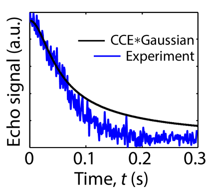
Figure 5.11: Calculations convolved with Gaussian $B$-field distribution of width 0.42 mT (arising from inhomogeneous broadening from the nuclear spin bath) show an excellent fit with the experimental Hahn echo decay around an ESR-type OWP ($B\sim 80$ mT), with no free fit parameters. Figure adapted from Balian et al. (2014) and the experimental data was first published in Wolfowicz et al. (2013).

5.4.5 Angular Dependence

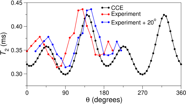
Figure 5.12: Angular dependence of $T_{2}$ for an ESR transition of Si:Bi. Rotation was performed about the $[\overline{1}\overline{1}2]$ axis in the $[\overline{1}10]$ - $[111]$ plane with $\theta$ from $[\overline{1}10]$. The best match to experiment was obtained for a $5^{\circ}$ tilt in the rotation axis and a zero-offset of $20^{\circ}$. Figure adapted from Balian et al. (2014).

The strength of the dipolar interaction $C_{12}$ depends on the angle between the vector joining the interacting spins and the direction of the magnetic field ${\bf B}$ as discussed in Section 2.4.2. As a result, $T_{2}$ varies with the orientation of the crystal sample relative to ${\bf B}$ (de Sousa and Das Sarma, 2003b; Witzel and Das Sarma, 2006; Tyryshkin et al., 2006; George et al., 2010).

$T_{2}$ was measured as a function of crystal orientation as shown in Figure 5.12. X-ray diffraction using the back-reflection Laue technique showed the rotation axis to be close to $[\overline{1}\overline{1}2]$. The external magnetic field is in the rotation plane, defined by the angle $\theta$ such that $\theta=0^{\circ}$ and $\theta=90^{\circ}$ correspond to the field parallel to $[\overline{1}10]$ and $[111]$ respectively. However, there are experimental uncertainties in both the initial angle $\theta=0^{\circ}$ and the position of the rotation axis. In order to determine the best crystal orientation to use in the simulations, CCE calculations as a function of orientation were compared with experimental measurements as shown in Figure 5.12. The best match to experiment was obtained for the rotation axis tilted about $[111]$ by $5^{\circ}$ from $[\overline{1}\overline{1}2]$, and a $20^{\circ}$ shift in $\theta$.

All the points in Figure 5.10 used $\theta=135^{\circ}$, except for the first point corresponding to the ESR-type OWP (smallest polarisation difference). A different sample with the field aligned along $[011]$ was used for the latter point. The bismuth donor concentration of the ESR-type OWP point was also different ($[\text{Bi}]=10^{16}$ cm^-3) from the rest of the points ($[\text{Bi}]=3\times 10^{15}$ cm^-3). The difference in [Bi] is not expected to affect coherence times in the regimes studied, which are not dominated by donor-donor effects.

5.4.6 Quantum Bath vs. Classical Noise

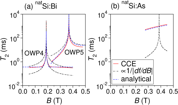
Figure 5.13: Shows that the hybrid qubit coherence time as a function of magnetic field ($T_{2}(B)$) is not necessarily inversely proportional to the frequency-field gradient $df/dB$. Red solid line is $T_{2}$ calculated using the cluster correlation expansion (CCE); black dotted-dashed line is $T_{2}\propto 1/(df/dB)$. (a) $T_{2}(B)$ around a typical ESR-type ‘optimal working point’ (OWP) of Si:Bi cannot be fitted by $df/dB$, except locally. The $df/dB$ lines have been rescaled to fit either the OWP region or the asymptotic regions; they cannot fit both. The blue dashed lines are calculated using the closed-form formula described in Chapter 6. (b) The single NMR-type ‘clock transition’ (CT) of Si:As at $B\simeq 0.39$ T (where $df/dB=0$), exemplifies a CT which is not an OWP (i.e. there is no enhancement in $T_{2}$). Si:Bi also has such CTs. Calculations were performed for the natural abundance of ²⁹Si (4.67%). Figure adapted from an earlier version of Balian et al. (2014) (arXiv:1302.1709v3 [cond-mat.mes-hall] (2013) ).

Classical noise models relate coherence times as a function of $B$ to various orders and powers of $df/dB$ (Vion et al., 2002; Ithier et al., 2005; Martinis et al., 2003; Mohammady et al., 2012; Wolfowicz et al., 2012, 2013):

$$(T_{2}(B))^{-1}=C\left\{\frac{df(B)}{dB},\left(\frac{df(B)}{dB}\right)^{2},\dots,\frac{d^{2}f(B)}{dB^{2}},\left(\frac{d^{2}f(B)}{dB^{2}}\right)^{2},\dots\right\},$$ (5.5)

where $C$ is a field-independent constant which in general depends on the central spin, bath and interaction Hamiltonians. The simplest of these is $T_{2}\propto 1/(df/dB)$. This treatment provides an intuitive interpretation of sweet-spots where $df/dB\simeq 0$; changes in the central-state splitting $\Delta f$ are insensitive to changes in magnetic field fluctuations $\Delta B$ and hence the initial superposition of the qubit has enhanced protection from noise. This argument is valid for random classical noise such as instrument noise. However, for the case of $\Delta B$ arising from a quantum spin environment, we find that $df/dB$ cannot account for the global $B$ dependence of $T_{2}$. This is illustrated for Si:Bi in Figure 5.13(a). It is only possible to fit $1/(df/dB)$ locally (for some $B$ range, but not all $B$) to CCE $T_{2}(B)$ curves.

Also shown in Figure 5.13 is that while some of the OWPs are coincident with CTs where $df/dB\rightarrow 0$, others (in particular the NMR-type OWPs) are not; such as the CT for Si:As in Figure 5.13(b). The reason for this deviation is that $\hat{H}_{\text{int}}$ differs from a magnetic field-type term ($\propto(S^{z}+\delta_{X}I_{X}^{z})$). In other words, while $\hat{H}_{\text{int}}$ determines the form of the interaction between the central spin system and the bath, it is $\hat{H}_{\text{CS}}$ which determines $df/dB$. If $\hat{H}_{\text{int}}$ and $\hat{H}_{\text{CS}}$ are of different form, then clock transitions are not OWPs. In the case of nuclear spin diffusion for Si:Bi systems, for $B\sim 1$ T, there is still sufficient mixing between the electronic and nuclear degrees of freedom so that it is the contact hyperfine interaction ($\propto S^{z}$ and not $\propto(S^{z}+\delta_{X}I_{X}^{z})$) which dominates the effect of $\hat{H}_{\text{int}}$, thus we may neglect the interaction between the bismuth nuclear spin and the bath, even for NMR-type transitions. However, in this range, the nuclear Zeeman term contributes significantly to $df/dB$ for NMR-type transitions (see Equation (3.24) for an exact expression for $df/dB$).

5.5 Conclusion

In summary, we presented coherence times of the hybrid qubit in the natural silicon spin bath, calculated using the CCE, and in numerous parameter regimes; these are for magnetic fields near and far from OWPs (the latter in the unmixed regime), both for ESR-type and NMR-type transitions (Balian et al., 2014, 2015), and also for ESR-forbidden transitions (Morley et al., 2013). In all cases, our numerical calculations are in good agreement with experiments.

The coherence times we reported for the hybrid qubit at $S$-band forbidden transitions (Morley et al., 2013) can be longer than those of the pure electron but are shorter than for the case of a nucleus. The coherence times are five orders of magnitude longer than the timescale for manipulation (32 ns manipulation time as described in Chapter 3). Without OWPs, the relevant coherence time for quantum computation with the hybrid qubit is the shortest one; that of the pure electron spin. The longest qubit manipulation time is that of the pure nucleus and dominates the time taken for a quantum computation. Thus, the hybrid qubit at $S$-band offers the possibility of preventing the ‘worst of both worlds’: the limiting coherence time is at least as long while the manipulation time is enhanced by orders of magnitude.

We further presented the first demonstration of suppression of spin bath decoherence at OWPs (Balian et al., 2012), later verified by experiments (Wolfowicz et al., 2013; Balian et al., 2014). Near an ESR-type OWP, coherence times of the hybrid qubit in natural silicon are increased from about 0.5 ms to 100 ms. Here, quantum control can also be achieved with fast ns pulses, as the transition matrix element is primarily electronic.

An underlying question of physical interest is when decoherence is the result of the magnetic noise from independently flip-flopping pairs of spins and when consideration of the many-body nature of the quantum bath is important. The answer is also of use for practical reasons. For one, if decoherence is due to flip-flopping pairs, there are widely used models (such as the analytical pseudospin expressions in Chapter 6) which can be used to accurately calculate decays. Otherwise, more complex many-body numerics become essential to simulate and fully understand experimental behaviours. The clear result is that for the Hahn spin echo (and also for low to moderate pulsed dynamical decoupling as will be seen in Chapter 7), the elimination of correlations from independent pairs is so drastic at OWPs, that many-body numerics (CCE3) is almost indispensable for full understanding and accuracy (Balian et al., 2015).

In summary, for the FID and Hahn spin echo, the latter in regions away from OWPs, pair correlations give converged coherence decays and hence a reliable $T_{2}$ can be extracted. Near OWPs, the Hahn echo only decays for an initial time period much shorter than the timescale of $T_{2}$, however, extrapolating the short-time behaviour for long times gives the correct timescale. The experiments we compare to are all for the Hahn echo, and the short-time pair correlations give the correct $T_{2}$. We find that up to three spin clusters are needed to achieve converged CCE Hahn echo decays near OWPs. These higher-order CCE results are in agreement with our pair correlation results for the short-time Hahn (and the analytical formula described in Chapter 6).

Finally, we illustrated the significant differences between decoherence from classical field noise and quantum bath decoherence by comparing our CCE calculations to $df/dB$ models (Balian et al., 2014). The content we present in the next chapter further illustrates such differences and clear signatures of quantum bath decoherence, by analysing pair correlations and deriving a closed-form $T_{2}$ formula for the hybrid qubit in a nuclear spin bath.

6  |  Hybrid Pseudospins
and $T_{2}$ Formula

In this chapter, we present a derivation for a closed-form $T_{2}$ formula for nuclear spin diffusion of the hybrid qubit, first published in Balian et al. (2014). The formula also clarifies significant differences between decoherence driven by classical field noise and quantum bath decoherence. In order to obtain the formula, we analyse the pair correlations for the single-spin FID case. We then numerically establish the relationship between the Hahn spin echo and single-spin FID, scaling the formula to account for the Hahn spin echo case and compare its predictions with experiments for the Hahn spin echo.

The formula also clearly exposes qualitative differences between decoherence driven by a quantum spin bath and decoherence due to classical magnetic field fluctuations. We derive the formula by showing that the spin dynamics separate naturally into terms acting on very different timescales. The formula is valid for the hybrid qubit in both the mixed and unmixed regimes, the latter corresponding to a bare electron spin. The coherence time is given as a function of the polarisation (for each level and as described in Chapter 3) which quantifies the mixing as a simple analytical function of $B$. The formula is

$$T^{u\to l}_{2}(B,\theta)\simeq\overline{C}(\theta)\frac{|P_{u}(B)|+|P_{l}(B)|}{\left|P_{u}(B)-P_{l}(B)\right|},$$ (6.1)

written for a transition $\left|{u}\right\rangle\to\left|{l}\right\rangle$ at magnetic field $B$. The constant, $\overline{C}(\theta)$, depends only on magnetic field orientation, the density of nuclear spin impurities and their gyromagnetic ratio. Equation (6.1) is shown to give excellent agreement with CCE numerics and experimental data for both ESR-type and NMR-type transitions near and far from OWP regimes.

6.1 Hybrid Pseudospins

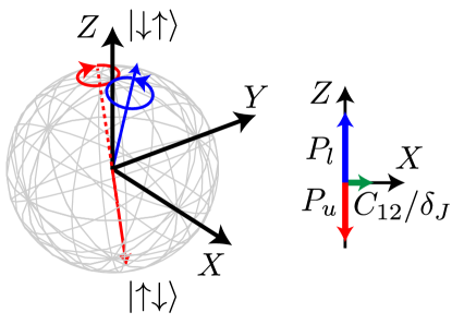
Figure 6.1: Illustration of the evolution of the bath states in the Hilbert space spanned by $\{\left|{\uparrow\downarrow}\right\rangle,\left|{\downarrow\uparrow}\right\rangle\}$ under the influence of their dipole coupling ($C_{12}$) and their mutual detuning $\delta_{J}$ caused by interaction with the central spin. Figure adapted from Balian et al. (2014).

In order to investigate the suppression of decoherence at OWPs and also for fields and transitions far from OWPs, here we analyse only pair correlations which can be treated as independent pseudospins as explained in Section 2.5.5. For the case of the FID at all magnetic fields and in unmixed regimes far from OWPs for both the FID and Hahn spin echo, CCE2 gives convergent decays and so an analysis based on pseudospins is fully justified. Near OWPs however, the Hahn spin echo only decays for some initial time and higher-order numerics are needed for converged decays as was shown in Chapter 5. However, the initial decay of the Hahn echo gives a good indication of the $T_{2}$ timescale. All our pseudospin results agree with experimental measurements of $T_{2}$ for the Hahn echo near OWPs in this early-decay approximation.

6.1.1 Interaction and Bath Hamiltonians

For donors spin qubits in silicon, one may assume $H_{\text{CS}}\gg H_{\text{bath}}$ and thus ignore non-secular terms in $\hat{H}_{\text{int}}$. The interaction Hamiltonian Equation (2.21) for the $n$-th pair reduces to Ising form:

$$\hat{H}^{(n)}_{\text{int}}=\sum_{a=1,2}J^{(n)}_{a}\hat{S}^{z}\hat{I}^{z}_{i},$$ (6.2)

with Fermi contact hyperfine coupling strengths $J^{(n)}_{a}$. For the two interacting spin-1/2 bath spins, assuming a large magnetic field and thus keeping only energy conserving terms, the dipolar interaction in Equation (2.19) simplifies to

$$\hat{H}^{(n)}_{\text{bath}}=C^{(n)}_{12}\hat{I}_{1}^{z}\hat{I}_{2}^{z}-\tfrac{C^{(n)}_{12}}{4}(\hat{I}_{1}^{+}\hat{I}_{2}^{-}+\hat{I}_{1}^{-}\hat{I}_{2}^{+})$$ (6.3)

where $C^{(n)}_{12}$ is the strength of the dipolar coupling between the two bath spins for pair $n$. Zeeman terms are also excluded from $\hat{H}^{(n)}_{\text{bath}}$ as these do not contribute to decoherence. Neglecting the effect of $\hat{H}_{\text{int}}$ on the mixing of the central spin states, the dynamics is governed by $\hat{h}^{(n)}_{i}$ (conditional on the state of the central spin):

$$\hat{h}^{(n)}_{i}\equiv\left\langle{i}\right|(\hat{H}_{\text{int}}^{(n)}+\hat{H}_{\text{bath}}^{(n)})\left|{i}\right\rangle=-\tfrac{C_{12}}{4}\hat{\mathds{1}}-\tfrac{1}{4}\hat{\bm{\sigma}}\cdot{\bf H}^{(n)}_{i},$$ (6.4)

where the effective field is ${\bf H}^{(n)}_{i}=[C^{(n)}_{12},0,P_{i}\delta_{J}^{(n)}]$. Here, $\delta_{J}^{(n)}\equiv(J^{(n)}_{1}-J^{(n)}_{2})$ is the difference in hyperfine couplings to the bath while $\hat{\bm{\sigma}}$ is the vector of Pauli matrices acting on the bath basis $\{\left|{\downarrow\uparrow}\right\rangle\equiv\left|{\downarrow}\right\rangle\otimes\left|{\uparrow}\right\rangle,\left|{\uparrow\downarrow}\right\rangle\equiv\left|{\uparrow}\right\rangle\otimes\left|{\downarrow}\right\rangle\}$ and $\left|{\uparrow}\right\rangle$ and $\left|{\downarrow}\right\rangle$ denote the nuclear spin-1/2 Zeeman states. The identity term is dynamically uninteresting; the dynamics can in fact be considered simply as a precession about ${\bf H}_{i}^{(n)}$. Diagonalising the Hamiltonians in Equation (6.4) gives the pseudospin precession rates

$$\omega_{i}^{(n)}=\frac{1}{4}\sqrt{(C_{12}^{(n)})^{2}+(P_{i}\delta_{J}^{(n)})^{2}},$$ (6.5)

while the angle of ${\bf H}_{i}^{(n)}$ from the $z$-axis is

$$\theta_{i}^{(n)}=\tan^{-1}{[C_{12}^{(n)}/(P_{i}\delta_{J}^{(n)})]}.$$ (6.6)

The pseudospins are illustrated in Figure 6.1.

For the hybrid qubit, the pseudospin dynamics is in most respects, quite similar to those investigated previously for electron (unmixed) qubits (Yang and Liu, 2008a, b, 2009; Yao et al., 2006, 2007; Liu et al., 2007; Zhao et al., 2012a). However, the main difference is that for our case, the hybrid pseudospins have the electron $z$-projection $\hat{S}^{z}$ replaced by the polarisation term $P_{i}\equiv 2\left\langle{i}\right|\hat{S}^{z}\left|{i}\right\rangle$. While for an electron, $P_{i}=\pm 1$ is a constant, for mixed systems the $P_{i}(B)$ are strongly field-dependent. The pseudospin analysis is framed in the pure dephasing approximation and hence requires that the interaction Hamiltonian has negligible effect on the mixing of the central spin states themselves, i.e. on $P_{i}$. Since $H_{\text{CS}}\gg H_{\text{int}}$, this is the case except extremely close to OWPs, where $T_{2}$ becomes extremely sensitive to small fluctuations in $P_{i}$.

6.2 Derivation of $T_{2}$ Formula

We employ an analysis of the hybrid pseudospins and a range of other approximations described below to derive the formula. The analysis also provides an intuitive picture of the system-bath dynamics, especially with respect to the magnetic field approaching an OWP and far from it, and also for NMR-type and ESR-type transitions.

6.2.1 Short-Time Behaviour

The $n$-th cluster decay for a single spin pair $n$ has been investigated analytically for both the FID and Hahn echo case (Yao et al., 2006; Zhao et al., 2012a; Witzel et al., 2005). We emphasize that this is the single-spin FID without inhomogeneous broadening. In experiment, $T_{2}$ is normally measured using a Hahn echo pulse sequence, in order to remove strong enhancements in decoherence arising from static inhomogeneities. Although the Hahn echo can suppress some effects of the dynamics, the FID and Hahn $T_{2}$ times are of the same order, differing by at most a factor of $\approx 2$ even at OWPs, so we focus our analysis on the simpler FID expressions.

Although analytical forms for the time decays $\mathcal{L}_{n}^{u\to l}(t)$ from spin pairs are known (Yao et al., 2007; Zhao et al., 2012a), a closed form for $T_{2}$, sufficiently accurate for experimental analysis is more difficult. Each $\mathcal{L}^{u\to l}_{n}(t)$ is an oscillatory function, with frequencies given in terms of $\omega_{u}^{(n)}$ and $\omega_{l}^{(n)}$ and the full decays combines hundreds or thousands of spin pair contributions.

A usual approach is to expand the decay as a power series $|\mathcal{L}_{n}^{u\to l}(t)|=1-\sum_{p=1}a^{(n)}_{2p}t^{2p}$ and to infer the order of magnitude of $T_{2}$ from the early time behaviour. However, for important cases like spin diffusion, $a_{2}^{(n)}=0$ while $a^{(n)}_{4}\neq 0$, predicting a $\exp[-a^{(n)}_{4}t^{4}]$ decay to leading order (Witzel et al., 2005; Yao et al., 2006, 2007), in contrast to the observed decays of $\sim\exp[-a^{(n)}_{2}t^{2}]$ for typical spin systems, where the Taylor coefficient $a^{(n)}_{2}$ is identified as $1/T_{2}^{2}$ . Thus it appears that in that case, one cannot infer the character of the decay on timescales $t\sim T_{2}$ from the short time behaviour (i.e. on timescales $t\sim\omega_{i}^{-1}$).

The observed exponential-quadratic (Gaussian) character of the coherence decay has been demonstrated numerically for both Hahn echo decay and FID from cluster expansion or linked-cluster expansion simulations (Witzel and Das Sarma, 2006; Saikin et al., 2007). For the FID case specifically, a crossover from the exponential-quartic to Gaussian behaviour was found on the microsecond timescale, arising from the combined effect of many pair cluster contributions (Saikin et al., 2007). For spin donors in silicon, $T_{2}$ times are on the millisecond to second timescales, thus the exponential-quartic regime is not relevant (though it may be appropriate for GaAs quantum dots, which have shorter $T_{2}$ times).

Below, we shall see that $T_{2}$ times sufficiently reliable for experimental analysis are obtainable analytically if we consider, separately, the different frequency terms involved in the pair correlation which act on very different timescales. Thus, we propose a very different explanation for the observed decay form crossover in the FID which does not require one to combine large numbers of cluster contributions. We show that in fact the crossover originates naturally from a single pair correlation term.

6.2.2 Bath State Overlap

As discussed in Chapter 2, the decay in coherence of the central spin can be related to its entanglement with the bath. We assume an initial state such that the qubit and bath are unentangled, and the qubit is prepared in a coherent superposition of its upper ($\left|{i=u}\right\rangle$) and lower ($\left|{i=l}\right\rangle$) states. The coherence for the FID in pure dephasing for the $n$-th spin pair is given by

$$|\mathcal{L}^{u\to l}_{\text{FID},n}(|\mathcal{B}^{(n)}(0),t)\rangle|=|\langle\mathcal{B}^{(n)}_{u}(t)|\mathcal{B}^{(n)}_{l}(t)|=\langle\mathcal{B}^{(n)}_{l}(0)|\hat{T}^{(n)\dagger}_{u}\hat{T}^{(n)}_{l}|\mathcal{B}^{(n)}_{u}(0)\rangle|,$$ (6.7)

which involves calculating the time-dependent overlap between bath states correlated with the upper and the lower central spin states.

For simplicity, we drop the pair label $n$ in what will follow until summing the contribution from all spin pairs. The evolution of the bath during the FID of the central spin follows $\bm{\mathcal{B}}_{i}(t)={\bf R}_{y}(\theta_{i}){\bf R}_{z}(2\omega_{i}t){\bf R}_{y}^{\intercal}(\theta_{i})\bm{\mathcal{B}}(0)$ in the matrix representation, where ${\bf R}_{y}$ and ${\bf R}_{z}$ represent the usual rotation matrices (Nielsen and Chuang, 2010) and $\bm{\mathcal{B}}(0)$ is the initial bath state in the basis $\{{(0\ 1)}^{\intercal}:\left|{\uparrow\downarrow}\right\rangle,{(1\ 0)}^{\intercal}:\left|{\downarrow\uparrow}\right\rangle\}$ and in general can be a superposition of $\left|{\uparrow\downarrow}\right\rangle$ and $\left|{\downarrow\uparrow}\right\rangle$. We can combine the unitaries for the upper and lower state in one matrix and thus the bath overlap can be written as

$$\mathcal{L}_{\text{FID}}^{u\to l}(t)=\bm{\mathcal{B}}^{\intercal}(0){\bf T}^{*}_{ul}(\omega^{-},\omega^{+},t)\bm{\mathcal{B}}(0);$$

$${\bf T}^{*}_{ul}(\omega^{-},\omega^{+},t)=$$ (6.8)

$${\bf R}_{y}(\theta_{u})\left(\begin{array}[]{cc}e^{i\omega^{-}t}\cos{\theta^{-}}&e^{i\omega^{+}t}\sin{\theta^{-}}\\ -e^{-i\omega^{+}t}\sin{\theta^{-}}&e^{-i\omega^{-}t}\cos{\theta^{-}}\end{array}\right){\bf R}_{y}^{\intercal}(\theta_{l})$$ (6.11)

where $\theta^{\pm}=\frac{1}{2}(\theta_{u}\pm\theta_{l})$ and $\omega^{\pm}=\omega_{u}\pm\omega_{l}$. We see that expressions for the decays arise naturally in terms of $\omega^{\pm}$ rather than $\omega_{u}$ and $\omega_{l}$ as is usual.

For the initial state $\bm{\mathcal{B}}(0)^{\intercal}={(0\ 1)}$ or ${(1\ 0)}$, the time decay for FID is given by

$$|\mathcal{L}^{u\to l}_{\text{FID}}(\left|{\uparrow\downarrow}\right\rangle,t)| =|\{{\bf T}^{*}_{ul}(\omega^{-},\omega^{+},t)\}_{11}|$$

$$=\left|D^{+}e^{-i\omega^{-}t}+D^{-}e^{+i\omega^{-}t}\leavevmode\nobreak\ \leavevmode\nobreak\ +R^{+}e^{-i\omega^{+}t}+R^{-}e^{+i\omega^{+}t}\right|,$$ (6.12)

where $R^{\pm}=\frac{1}{2}\sin\theta^{-}(\sin\theta^{-}\mp\sin\theta^{+})$ while $D^{\pm}=\frac{1}{2}\cos\theta^{-}(\cos\theta^{-}\pm\cos\theta^{+})$.

6.2.3 $T_{2}$ Weights from Pairs

We now consider the contributions to the coherence which dominate the spin pair correlation in different regimes and timescales. We consider Equation (6.12) in three principal limits:

1. For an ESR-type transition in the high-field regime in which the states are not mixed. This corresponds to $P_{u}\simeq-P_{l}$.

2. For an NMR-type transition in the high-field regime, or for any transition near an OWP. Here, $P_{u}\simeq P_{l}$.

3. For an intermediate regime corresponding to a Landau-Zener crossing (Mohammady et al., 2010) or cancellation resonance, where one of the $P_{i}\simeq 0$.

The pseudospin evolutions for the first two regimes are illustrated in Figure 6.2

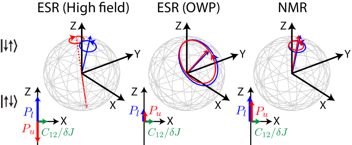
Figure 6.2: Illustration of the evolution of the bath states in the Hilbert space spanned by $\{\left|{\uparrow\downarrow}\right\rangle,\left|{\downarrow\uparrow}\right\rangle\}$ under the influence of their dipole coupling ($C_{12}$) and their mutual detuning caused by interaction with the central spin. At both OWPs and NMR-type transitions, bath trajectories correlated with the upper and lower central spin states follow similar trajectories and hence decoherence is suppressed compared to ESR-type transitions. However, at ESR-type OWPs, $|P_{u,l}|\simeq 0.1$ leads to a larger trajectory and proportionately shorter $T_{2}$ values relative to NMR-type transitions. Figure adapted from Balian et al. (2014).

For either (i) or (ii), since $|P_{u}|\simeq|P_{l}|$ then $\omega_{u}\simeq\omega_{l}$ and thus $\omega^{+}/\omega^{-}\gg 1$. Hence, we infer that the $R^{\pm}$ terms act on very different timescales from the terms proportional to $D^{\pm}$. We consider the $R^{\pm}$ and $D^{\pm}$ terms separately. If we set $\omega^{-}=0$, we obtain the fast oscillating contribution:

$$|\mathcal{L}^{u\to l}_{\text{FID}}(\left|{\uparrow\downarrow}\right\rangle,t)|^{2}\simeq 1-4\left(D^{+}+D^{-}\right)\left(R^{+}+R^{-}\right)\sin^{2}\tfrac{\omega^{+}t}{2}-4R^{+}R^{-}\sin^{2}(\omega^{+}t).$$ (6.13)

We now extract the contribution of each cluster to the total decoherence by means of a power expansion; for short times we obtain

$$|\mathcal{L}_{\text{FID}}^{u\to l}(\left|{\uparrow\downarrow}\right\rangle,t)|^{2}\approx 1-\frac{t^{2}}{T_{2}^{2}}\approx\exp{\left[-\left(\frac{t}{T_{2}}\right)^{2}\right]},$$ (6.14)

yielding the $n$-th cluster contribution to $T_{2}$:

$$\left(T^{(n)}_{2}\right)^{-2}\approx\left[\left(D^{+}+D^{-}\right)\left(R^{+}+R^{-}\right)+4R^{+}R^{-}\right]\left(\omega^{+}\right)^{2}.$$ (6.15)

We now perform the incoherent averaging over initial bath states, $\left\langle\mathcal{L}^{u\to l}_{\text{FID}}(t)\right\rangle\approx\tfrac{1}{2}+\tfrac{1}{2}|\mathcal{L}^{u\to l}_{\text{FID}}(\left|{\uparrow\downarrow}\right\rangle,t)|$ to allow for the fact that approximately half the bath spins are in $\left|{\uparrow\uparrow}\right\rangle$ and $\left|{\downarrow\downarrow}\right\rangle$ states which cannot flip-flop and obtain:

$$\frac{1}{T_{2}^{(n)}}\simeq\frac{1}{2}\left|\sin\theta_{u}-\sin\theta_{l}\right|\frac{\omega^{+}}{2},$$ (6.16)

noting that the first term is the difference in precession radii of the pseudospins, while the second term denotes the average precession rate. In terms of the usual flip-flop models, we note that a larger precession radius corresponds to a larger flip-flop amplitude, while a larger precession frequency corresponds to a higher flip-flop frequency.

6.2.4 Separation of Timescales

We now distinguish between the two regimes (i) and (ii). For (i), for timescales $\ll(\omega^{+})^{-1}$, as discussed above, we neglect the slow oscillations (i.e. those in $\omega^{-}$) in Equation (6.12), which contribute only on very long timescales. We obtain the $n$-th cluster contribution to $T_{2}$ (Equation (6.16)) by Taylor expanding the decay with $\omega^{-}$ set to zero, i.e. using only the fast terms. For (ii), $\omega^{+}/\omega^{-}\gg 1$ is still valid but $|D^{\pm}|\gg|R^{\pm}|$ in Equation (6.12), and the slow oscillations dominate for timescales $1/\omega^{+}\lesssim t\lesssim 1/\omega^{-}$. However, expanding these slow oscillations gives precisely the same form as Equation (6.16).

Using Equation (6.16) in all cases, we can estimate a total $T_{2}$ using

$$\frac{1}{T_{2}^{2}}=\sum_{n=1}^{n=N}\left(\frac{1}{T_{2}^{(n)}}\right)^{2},$$ (6.17)

where for the converged CCE2 spin bath in natural silicon, $N\simeq 10^{4}$.

Importantly, including both fast ($\omega^{+}$) and slow ($\omega^{-}$) terms the power series (i.e. expanding the full decay Equation (6.12)), the quadratic contributions cancel and the pair correlation result simply gives an exponential-quartic dependence (not observed in experiment) at leading order. Separation of the $\omega^{\pm}$ timescales is useful not only here, but also potentially in the unmixed ESR regimes of other spin systems. We proceed to discuss the importance of separating timescales further.

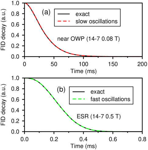
Figure 6.3: Shows that OWP regimes are dominated by slow oscillating terms while ESR regimes are dominated by fast oscillating terms in Equation (6.12). (a) Compares decays obtained from Equation (6.12) (exact) with decays obtained from Equation (6.18) (slow oscillations only). (b) Compares decays obtained from Equation (6.12) (exact) with decays obtained from Equation (6.13) (fast oscillations only). Figure adapted from Balian et al. (2014).

As mentioned above, care is needed when considering the (ii) regimes (OWP and NMR) since here, $P_{u}\simeq P_{l}$ and $\theta_{u}\simeq\theta_{l}$ and thus $D^{\pm}\gg R^{\pm}$. Here, $D^{+}+D^{-}\to 1$ while $R^{\pm}\to 0$. Decay timescales become long and comparable to $1/\omega^{-}$ while the $R^{\pm}$ amplitudes are negligible and thus the slow oscillating components are important. In that case, we would, in contrast to Equation (6.13), neglect the fast oscillations. Then we obtain,

$$|\mathcal{L}^{u\to l}_{\text{FID}}(\left|{\uparrow\downarrow}\right\rangle,t)|^{2}\simeq 1-4D^{+}D^{-}\sin^{2}\omega^{-}t.$$ (6.18)

In this case, $(T_{2}^{(n)})^{-2}\approx D^{+}D^{-}\left(\omega^{-}\right)^{2}$. However, since

$$\left[\left(D^{+}+D^{-}\right)\left(R^{+}+R^{-}\right)+4R^{+}R^{-}\right]\left(\omega^{+}\right)^{2}\to D^{+}D^{-}\left(\omega^{-}\right)^{2}$$ (6.19)

as $P_{u}\to P_{l}$, the contribution to $1/T_{2}^{2}$ from each cluster, in fact, still has the same form as Equation (6.15). In other words, the relative weights obtained from the slow, high-amplitude contributions are quite similar to those obtained by considering the faster, lower oscillations and thus the $T_{2}$ expression we derive below is still valid.

In Figure 6.3, we show the full temporal decay for all pairs

$$\mathcal{L}_{\text{FID}}^{u\to l}(\left|{\uparrow\downarrow}\right\rangle,t)=\prod_{n}^{N\simeq 10^{4}}\mathcal{L}^{u\to l}_{\text{FID},n}(\left|{\uparrow\downarrow}\right\rangle,t),$$ (6.20)

where $\mathcal{L}^{u\to l}_{\text{FID},n}(\left|{\uparrow\downarrow}\right\rangle,t)$ are given by Equation (6.12) and compare with the slow terms in an OWP regime (Figure 6.3(a)) where $\mathcal{L}^{u\to l}_{\text{FID},n}(\left|{\uparrow\downarrow}\right\rangle,t)$ are given by Equation (6.18) and the fast terms in the ESR regime (Figure 6.3(b)) where $\mathcal{L}^{u\to l}_{\text{FID},n}(\left|{\uparrow\downarrow}\right\rangle,t)$ are given by Equation (6.13). Figure 6.3 shows that while the fast terms completely dominate coherence decay in the ESR regime, the slow terms completely dominate the decays in the OWP/NMR regime yet the form of the weights in the power expansion is similar: if added, the two contributions thus cancel (albeit briefly) yielding the quartic-exponential decay. This decay is of course valid on extremely short timescales $t\ll(\omega^{+})^{-1}$ but not on the $T_{2}$ timescale.

In fact, the fast oscillation behaviour is not entirely straightforward. For the slow oscillations, Equation (6.18) involves a single frequency and an approximate $\exp{[-(t/T_{2})^{2}]}$ decay is straightforwardly inferred. For the fast oscillations however, Equation (6.13) may be rewritten as follows for each spin pair:

$$|\mathcal{L}^{u\to l}_{\text{FID}}(\left|{\uparrow\downarrow}\right\rangle,t)|^{2} \simeq 1-\sin^{2}\theta^{-}\cos^{2}\theta^{+}\sin^{2}(\omega^{+}t)$$

$$- \sin^{2}2\theta^{-}\sin^{2}\tfrac{\omega^{+}t}{2}$$

$$- \frac{1}{4}\sin^{2}2\theta^{-}\sin^{2}(\omega^{+}t)$$

$$= 1-L_{s}(t)-\left(L_{l1}(t)-L_{l2}(t)\right).$$

We see that it combines three separate interfering terms, where $L_{l1}$ oscillates at half the frequency of the others. In fact, a power expansion of either one of the individual terms $L_{s}(t)$, $L_{l1}(t)$ and $L_{l2}(t)$ would yield the same weights expression Equation (6.16). It is the ubiquitous nature of this $\left(\sin\theta_{u}-\sin\theta_{l}\right)^{2}\left(\omega^{+}\right)^{2}$ term which underlies the robustness of the field dependence of our $T_{2}$ expression derived below.

We note that it is in fact the term $L_{s}(t)=\frac{1}{4}\left(\sin\theta_{u}-\sin\theta_{l}\right)^{2}(\omega^{+})^{2}$ which yields a quadratic dependence at short times. However, numerics show that it is the $1-(L_{l1}(t)+L_{l2}(t))$ terms which overwhelmingly determine the decay on longer $T_{2}$ timescales (but actually make little contribution on the $t\ll(\omega^{+})^{-1}$ timescale, where there is once again a brief cancellation of these near equal amplitude oscillations).

Finally we consider regimes (iii), or the Landau-Zener regimes (there are four such regions for Si:Bi). These do not fit the above analysis, which assumed $|P_{u}|\simeq|P_{l}|$. For the LZ points either $P_{u}\simeq 0$ or $P_{l}\simeq 0$. Thus, assuming $P_{u}\simeq 0$ we obtain,

$$|\mathcal{L}^{u\to l}_{\text{FID}}(\left|{\uparrow\downarrow}\right\rangle,t)|^{2}\simeq 1-\sin^{2}\theta_{u}\sin^{2}\omega_{u}t,$$ (6.22)

and hence for $t\ll(\omega_{u})^{-1}$, we have simply

$$|\mathcal{L}^{u\to l}_{\text{FID}}(\left|{\uparrow\downarrow}\right\rangle t)|^{2}\simeq 1-C_{12}^{2}t^{2}.$$ (6.23)

6.2.5 Strong Coupling Approximation

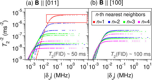
Figure 6.4: The individual contribution of each spin pair in the bath to the total $(1/T_{2})^{2}$ near OWPs, from Equation (6.16). Data are shown for two magnetic field orientations. For large $|\delta_{J}|$, coherence times become nearly independent of $|\delta_{J}|$. The scale of $T_{2}$ is set by a comparatively small $N\sim 10^{2}$ set of strongly-coupled spins ($|P_{i}\delta_{J}|\gg|C_{12}|$), illustrated in the red box. $B=79.8$ mT (about $0.1$ mT offset from the OWP) and $P_{i}\simeq 0.1$. $\gamma_{N}=8.465$ MHz/T for ²⁹Si and hyperfine coupling strengths were calculated using the Kohn-Luttinger electronic wavefunction with an ionization energy of $0.069$ eV for the bismuth electron (de Sousa and Das Sarma, 2003b). Figure adapted from Balian et al. (2014).

In Figure 6.4, we use Equation (6.16) to evaluate the strength of each ${}^{29}\text{Si}$ spin pair’s individual contributions to decoherence of a bismuth donor spin in silicon. We plot $1/(T_{2})^{2}$ for each cluster, as a function of $|\delta_{J}|$, in regime (ii) i.e. close to OWPs and NMR-type transitions. Strikingly, the spins are grouped into lines of constant $C_{12}$, corresponding to $n$-th nearest neighbor spins. Furthermore, for the spin pairs most active in driving decoherence, $1/(T_{2})^{2}$ is only very weakly dependent on $|\delta_{J}|$. The origin of this behaviour is clear from Equation (6.16): for large $|P_{i}\delta_{J}|\gg|C_{12}|$, the term $|\sin\theta_{u}-\sin\theta_{l}|\propto|\delta_{J}^{-1}|$ while $\omega^{+}\propto|\delta_{J}|$, eliminating the dependence on the hyperfine coupling between the central spin and bath spins.

The insensitivity of the decoherence to the coupling between the central spin and the bath might at first seem counter-intuitive. However, the physical origin of this effect is thus: increasing the hyperfine detuning $\propto|\delta_{J}^{-1}|$ damps the flip-flopping amplitudes; however within this model, the decrease in amplitude is exactly compensated by a corresponding increase in flip-flop frequency. We note that without separation of timescales, the exponential-quartic decay constants which prevail at times $t\ll\omega_{i}$ are dependent on $\delta_{J}^{2}$ (Yao et al., 2007). In contrast, our model predicts that a comparatively small number of strongly coupled spins will dominate the decoherence, and that their individual contributions to $1/T_{2}^{2}$ are approximately equal, although the individual coupling strengths $|\delta_{J}^{-1}|$ vary by orders of magnitude, ranging from $\sim 0.01$ to $10$ MHz.

To test the validity of this result at $t\sim T_{2}$ timescales, we ran CCE2 calculations for various field orientations. The dipolar coupling, $C_{12}$ is a function of the orientation $\theta$ of the magnetic field and hence the $T_{2}$ values vary accordingly. For $B\parallel\left\langle 011\right\rangle$, for example, the $N\sim 10^{2}$ strongest coupled spin pairs suffice to set the scale of $T_{2}$. We have tested our model by running a CCE2 calculation with just 120 nearest-neighbor (NN) spin pairs (e.g. for $B\parallel\left\langle 011\right\rangle$, $C_{12}^{\text{NN}}=2.4$ kHz) which satisfy $|P_{i}\delta_{J}|\gg|C_{12}|$, and confirming the calculated $T_{2}$ is approximately equal to that considering all $\approx 10^{4}$ spin pairs.

If we make the strong coupling approximation, the weights in Equation (6.16) can also be written as:

$$\frac{1}{(T_{2}^{(n)})^{2}}\simeq\frac{(\theta_{u}-\theta_{l})^{2}}{4^{2}}(\omega^{+})^{2}.$$ (6.24)

Then, noting $\theta_{i}\approx C_{12}/\omega_{i}$ and $\omega^{+}\approx\delta_{J}(|P_{u}|+|P_{l}|)$ we easily obtain $\frac{1}{T_{2}^{(n)}}\propto\frac{|P_{u}-P_{l}|}{|P_{u}|-|P_{l}|}$, for the cases (i) and (ii) when $|P_{u}|\simeq|P_{l}|$, which include both the unmixed ESR limit as well as the NMR and OWP limits. Summing the $T_{2}$ contributions according to Equation (6.17), our final $T_{2}$ expression is given by Equation (6.1): $T_{2}\simeq\overline{C}(\theta)\tfrac{|P_{u}|+|P_{l}|}{\left|P_{u}-P_{l}\right|}.$ For most orientations, $\overline{C}(\theta)\approx 4/(C_{12}^{\text{NN}}\sqrt{N})$. However, as the magnetic field orientation approaches $B\parallel\left\langle 100\right\rangle$, the contribution of nearest-neighbor ²⁹Si spin pairs vanishes, while 2nd and 3rd nearest neighbors contribute similarly. We discuss further details of the orientation dependence of $T_{2}$ in the next section.

Approaching the high magnetic field limit, ESR-type transitions occur between states where $P_{u}\simeq-P_{l}$, such that $T_{2}\simeq\overline{C}(\theta)$, while for NMR-type transitions as well as OWPs, $P_{u}\simeq P_{l}$, and decoherence by the nuclear spin bath is suppressed. Finally, for the third regime (iii) where one of the $P_{i}$ is zero, and hence the assumptions made to obtain Equation (6.1) are not valid. Nevertheless, starting from Equation (6.12) we obtain Equation (6.23) and after the usual bath average and sum over clusters, we find $T_{2}\sim\overline{C}(\theta)$ in this regime, and hence Equation (6.1) remains a reasonable approximation here.

6.3 Angular Dependence

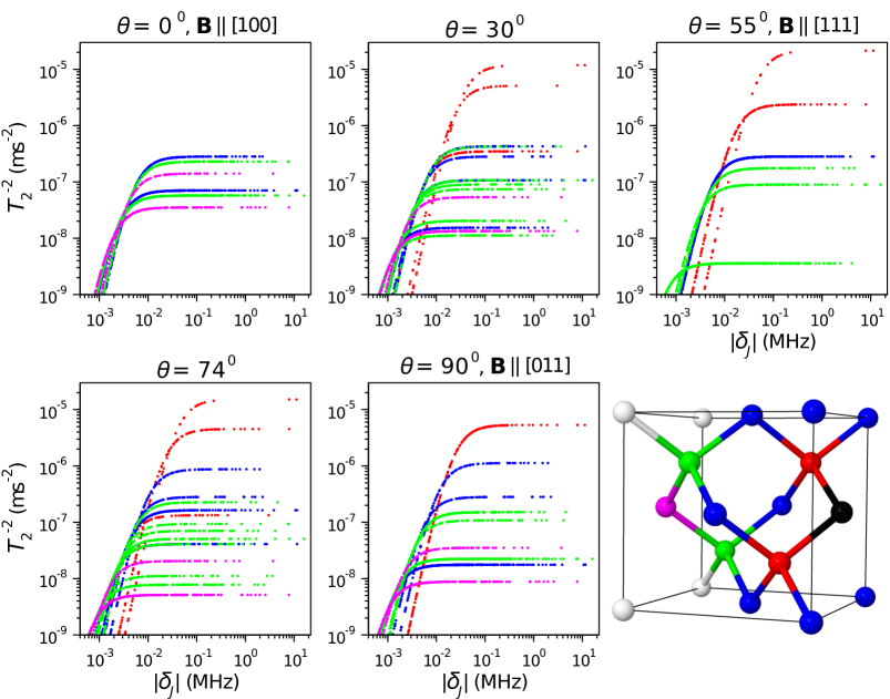
Figure 6.5: Theoretical contributions of spin pairs to $T_{2}(\text{Hahn})$, coloured according to $n$-th nearest neighbors relative to the black nucleus as illustrated in the last panel. First nearest neighbors dominate decoherence for rotation angles $\theta\gtrapprox 30^{\circ}$. At $\theta=0^{\circ}$, first nearest neighbor contributions are diminished and second and third nearest neighbors contribute the most to $T_{2}$. Rotation is performed about $\left[01\bar{1}\right]$ in the $\left[011\right]-\left[100\right]$ plane, with $\theta$ from $\left[100\right]$. Figure adapted from Balian et al. (2014). Details of the silicon crystal structure are given in Appendix C.

Rotation angle $\theta$	1-NN contribution to $\overline{C}(\theta)$	Numerical $\overline{C}(\theta)$
(degrees)	(ms)	(ms)
$90$	$0.37$	0.40
$74$	$0.35$	0.39
$55$	$0.32$	0.37
$30$	$0.41$	0.45
$0$	None. 2–NN, 3–NN contributions: $0.97$	$1.1$

Table 6.1: Numerical values of the dipolar prefactor $\overline{C}(\theta)$ compared to $\overline{C}(\theta)$ when including only nearest neighbor spin pairs, demonstrating that first nearest neighbors set the scale of $T_{2}$ for rotation angles $\theta\gtrapprox 30^{\circ}$. For $\theta=0^{\circ}$, 1–NNs do not contribute at all and 2,3–NNs largely determine $T_{2}$. The total number of strongest spin pairs for each orientation was chosen such that the $T_{2}$ obtained was about $70-80\%$ of the total $T_{2}$ when including all spin pairs in the bath. Rotation is performed about $\left[01\bar{1}\right]$ in the $\left[011\right]-\left[100\right]$ plane, with $\theta$ from $\left[100\right]$. Table adapted from Balian et al. (2014).

Due to angular dependence of the dipolar interaction, $T_{2}$ varies with the orientation of the crystal sample relative to ${\bf B}$ (de Sousa and Das Sarma, 2003b; Witzel and Das Sarma, 2006; Tyryshkin et al., 2006; George et al., 2010). The dipolar prefactor $\overline{C}(\theta)$ in our analytical $T_{2}$ formula (Equation (6.1)) depends on $C_{12}$ and is thus a function of crystal orientation. The prefactor is defined as

$$\overline{C}(\theta)=\frac{4}{\sqrt{\sum_{s}{N_{s}\left(C_{12}^{(s)}\right)^{2}}}},$$ (6.25)

where $s$ labels a unique value of spin pair dipolar strength $C_{12}^{(s)}$, or “shell”, which occurs $N_{s}$ times. We see below that including shells up to $s=3$ gives a good estimate of $\overline{C}(\theta)$, although for most angles $s=1$ suffices.

We now proceed to determine the full angular dependence of $\overline{C}(\theta)$. The various $1/T_{2}^{2}$ contributions of ²⁹Si spin pairs as a function of crystal rotation angle are shown in Figure 6.5. The data in Figure 6.5 was generated from Equation (6.16) near the ESR-type OWP (for rotation around the $\left[01\bar{1}\right]$ crystal direction) of Si:Bi in natural silicon, however, our results are independent of $B$ and the central donor species, up to a scaling factor on 1/$T_{2}^{2}$ contributions.

In Figure 6.5, the different shells are labelled according to whether the interacting spins are first, second, third or fourth nearest neighbors (1–, 2–, 3–, 4–NNs). The total $T_{2}$ is obtained by summing $1/T_{2}^{2}$ contributions from all spin pairs in the bath. We pick the strongest $N$ spin pairs (i.e., those with the largest $1/T_{2}^{2}$ contribution) such that the sum over $1/T_{2}^{2}$ is about $70-80\%$ of the total $T_{2}$, and find that $N\simeq 270$ for $\theta=0^{\circ}$ and $N\simeq 100$ for all the other rotations considered. Contributions from 1–NNs are dominant for $\theta\gtrapprox 30^{\circ}$. In Table 6.1, we show that 1–NNs suffice to set the scale of $T_{2}$ for $\theta\gtrapprox 30^{\circ}$ by comparing $\overline{C}(\theta)$ obtained from only 1–NNs to $\overline{C}(\theta)$ extracted from numerical CCE2 $T_{2}$ and using Equation (6.1). For $\theta=0^{\circ}$, 2–NNs and 3–NNs contribute the most, without any 1–NNs being involved in setting the scale of $T_{2}$. Including only the strongest 2–NN and 3-NN contributions, for $\theta=0^{\circ}$ we find $\overline{C}(0^{\circ})\simeq 0.97$ ms, compared to $\overline{C}(0^{\circ})=1.1$ ms obtained using the numerical $T_{2}$. Thus, using the estimated $\overline{C}(\theta)$ values in the first column of Table 6.1 provides a reasonable estimate of the dipolar prefactor $\overline{C}(\theta)$ as a function of crystal rotation.

6.4 Relating Hahn Spin Echo to FID

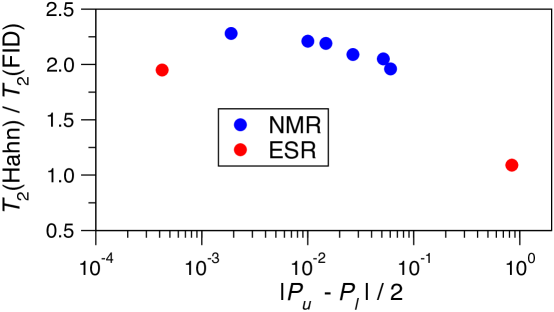
Figure 6.6: Comparison of calculated $T_{2}(\text{Hahn})$ and $T_{2}(\text{FID})$ for the various ESR-type and NMR-type transitions of Si:Bi for which $T_{2}$ was measured (Figure 6.8) covering a wide magnetic field range. Near OWPs (where $\left|P_{u}-P_{l}\right|\ll 1$), $T_{2}(\text{Hahn})/T_{2}(\text{FID})\simeq 2$. Figure adapted from Balian et al. (2014).

For the Hahn echo case, $\mathcal{L}^{u\to l}_{\text{Hahn}}(2t)=\bm{\mathcal{B}}(0)^{\intercal}{\bf T}^{*}_{ul}(\omega^{+},\omega^{-},t){\bf T}_{ul}(\omega^{+},\omega^{-},t)\bm{\mathcal{B}}(0)$, noting the exchange in order of $\omega^{\pm}$ relative to the FID case in Equation (6.11). The analysis for the Hahn case is less straightforward, but nevertheless for (ii), we estimate, using numerical CCE2 results at short-times, that near NMR-type transitions and OWPs, $T_{2}(\text{Hahn})\approx 2\times T_{2}(\text{FID})$, while $T_{2}(\text{Hahn})\approx T_{2}(\text{FID})$ elsewhere.

While FID and Hahn echo decays are generally of the same order, within about $5$ mT of an OWP, our calculated CCE2 Hahn echo (pair correlations) shows non-decaying behaviour at timescales beyond a few ms – as seen in Chapter 5. In contrast, the FID shows converged, near-Gaussian decays to zero intensity for all timescales and magnetic fields. Nevertheless, there is always a period of initial near-Gaussian decay for the Hahn echo near OWPs from which we extract $T_{2}(\text{Hahn})$. This initial period of convergence is extended to longer times as higher order cluster contributions are taken into account as shown in Chapter 5. We estimate numerically the ratio $T_{2}(\text{Hahn})/T_{2}(\text{FID})$ as shown in Figure 6.6 and find that

$$T_{2}(\text{Hahn})/T_{2}(\text{FID})\approx 2,$$ (6.26)

near OWPs (where $\left|P_{u}-P_{l}\right|\ll 1$). Far from OWPs, the coherence times are to within 10% as can be seen for the last ESR point in Figure 6.6 near $P_{u}-P_{l}\simeq 2$. In the previous chapter, we saw that fully-converged higher-order CCE calculations are in agreement with Equation (6.1) (with the factor of 2 scaling) and the short-time CCE2 results near OWPs.

6.5 Comparison with Frequency-Field Gradient

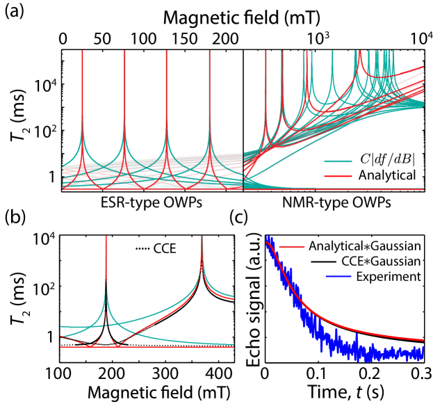
Figure 6.7: (a) The predicted $T_{2}$ values as a function of magnetic field for a variety of allowed transitions in Si:Bi, using Equation (6.1) derived in the text (labelled ‘analytical’), show eight OWPs where decoherence is suppressed. We also plot the magnetic field-frequency gradient ($df/dB$); though scaled by an arbitrary constant in order to match the range of estimated $T_{2}$ values, the discrepancies with Equation (6.1) are evident. In the left panel, transitions with no OWP are shown only faintly. (b) The analytical expression Equation (6.1) derived in the text is in good quantitative agreement with CCE2 numerics, but $df/dB$ is not. (c) Calculations convolved with Gaussian $B$-field distribution of width 0.42 mT (arising from inhomogeneous broadening from the nuclear spin bath) show an excellent fit with the experimental Hahn echo decay around an ESR-type OWP ($B\sim 80$ mT) (Wolfowicz et al., 2013), with no free fit parameters. Figure adapted from Balian et al. (2014).

We recall that the important mixing parameters $P_{i}$ in the $T_{2}$ formula (Equation (6.1)) may be evaluated analytically for an arbitrary donor species, for all field values. Also, the formula is perfectly valid for the case of a simple electronic spin (unmixed regime). In this section, we investigate deviations of our formula from the $T_{2}\sim df/dB$ dependence that one might expect from classical noise models. We also compare the predictions of the formula with numerical CCE calculations, and in the next section present comparisons with experiments. Also, we use the sensitivity of $T_{2}$ on magnetic field in the vicinity of OWPs (Balian et al., 2012) as a test of Equation (6.1). The parameters we use are for the bismuth donor in the ²⁹Si nuclear spin bath (in both mixed and unmixed regimes).

In Figure 6.7, we plot Equation (6.1) for Si:Bi for allowed ESR-type and NMR-type transitions across a range of magnetic fields. It shows close agreement with numerical CCE calculations including the effect of $\hat{H}_{\text{int}}$ on $P_{i}$ (i.e. with non-secular terms in $\hat{H}_{\text{int}}$ included). Both Equation (6.1) and CCE have distinctly different signatures from a curve proportional to $df/dB$, which would be expected in the case of classical field noise; and they cannot be fitted (except locally) by powers of $df/dB$. A comparison of Equation (6.1) with experiment is shown in Figure 6.7(c).

Figure 6.7(a) illustrates eight OWPs where $T_{2}\rightarrow\infty$: four ESR-type and four-NMR type transitions (these OWPs are all doublets, so there are in fact 16 separate OWP transitions). The form of Equation (6.1) clarifies the origin of these discrepancies. For low fields, ($B\lesssim 1$ T) the denominator of Equation (6.1) is $|P_{u}-P_{l}|\approx df/dB$. Thus, it is the numerator ($|P_{u}|+|P_{l}|$), which accounts largely for the deviation from the form expected for analogous classical noise ($T_{2}\propto 1/(df/dB)$).

At higher fields (left panel of Figure 6.7(a)), we see that the formula does not coincide with the ‘false positives’ of CTs (where $df/dB\rightarrow 0$). The reason of such false predictions of suppression of decoherence by CTs was given in Chapter 5. In Figure 5.13(b), it can be seen that the formula is in agreement with CCE (no suppression), while $df/dB$ predicts suppression of decoherence.

In summary, in Equation (6.1), it is the denominator ($|P_{u}-P_{l}|$) which sets the position of the OWPs: at these points the bath evolution becomes independent of the state ($\left|{u}\right\rangle$ or $\left|{l}\right\rangle$) of the central spin, and so the system-bath entanglement is zero (Figure 6.2). However it is the numerator (which can vary by an order of magnitude in the range $0\leq B\leq 1$ T) which provides the most distinct signature of the “back-action” between the quantum bath and central spin.

6.6 Comparison with Experiments

In this section the formula is compared with the experimental data already presented in Chapter 5 for the hybrid qubit near and far from OWPs and for both ESR-type and NMR-type transitions (Figure 5.10), obtained for Si:Bi in natural silicon. The experimental data was collected by Dr. Gary Wolfowicz and Professor John Morton at UCL.

Figure 6.8 shows $T_{2}$ measurements of ESR-type transitions towards the high-field regime, where $|P_{u}-P_{l}|\simeq 2$, and $T_{2}$ for a variety of different NMR-type transitions where $|P_{u}-P_{l}|$ varies by two orders of magnitude. It can be seen that the formula gives excellent agreement with the measured values. The primary variation in $T_{2}$ is due to the $|P_{u}-P_{l}|$ term; this is divided out in the lower panel of Figure 6.8, where the additional variations due to $|P_{u}|+|P_{l}|$ are apparent in the experiment.

As discussed in Chapter 5, the donor ESR line is inhomogeneously broadened by unresolved coupling to ²⁹Si, leading to an effective Gaussian magnetic field variation across the ensemble (FWHM of $0.42$ mT for Si:Bi in natural silicon). Therefore, to predict the measured $T_{2}$ at an ESR-type OWP, we convolve Equation (6.1) with the corresponding Gaussian magnetic field profile – Equation (5.4) with $\mathcal{L}_{B}(t)$ replaced by $e^{-\left(t/T_{2}\right)^{2}}$, where $T_{2}$ is given by Equation (6.1) and $B=B_{\text{OWP}}$. The convolution $D(t)$ is found to give a non-Gaussian decay, and reaches its $e^{-1}$ value at $100$ ms as shown in Figure 6.7(c), in close agreement with the experimental value of $93$ ms for the Si:Bi $\left|{14}\right\rangle\to\left|{7}\right\rangle$ OWP (Wolfowicz et al., 2013). The convolution sums $T_{2}(B)$ contributions which vary over orders of magnitude and thus represents a sensitive test of Equation (6.1) around an ESR-type OWP.

Equation (6.1) gives divergent $T_{2}$ values at the OWP; comparison with CCE indicates that it becomes unreliable within $\sim 0.01$ mT of the OWP and non-secular terms cap the maximum $T_{2}\lesssim 10$ s. However, the inhomogeneous broadening enables us to use Equation (6.1) to predict the measured (finite) $T_{2}$ at an ESR-type OWP by the convolution described above.

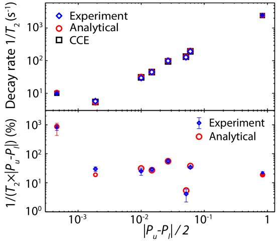
Figure 6.8: Comparison between theoretically predicted and measured $T_{2}$ in ^natSi:Bi for various transitions, showing remarkable agreement across a wide range of mixing regimes $|P_{u}-P_{l}|$. The label ‘analytical’ refers to Equation (6.1). Measurements were made at 4.8 K using ESR with a microwave frequency of 9.77 or 7.03 GHz (filled symbols), or electron-nuclear double resonance (ENDOR) between 200 MHz and 1 GHz using the method described in Morton et al. (2008) (empty symbols), at magnetic fields between 100 and 450 mT. These parameters are all in the regime where $|P_{u}-P_{l}|\approx df/dB$. The Bi donor concentration was $\leq 10^{16}$ cm^-3, and coherence times are limited by ²⁹Si spin diffusion. The theoretical points are based on a predicted value for $\overline{C}(\theta)=0.42$ ms. In the lower panel, the decay rates are normalised by $|P_{u}-P_{l}|$ to highlight the effect of $|P_{u}|+|P_{l}|$, and shown relative to the case when $|P_{u}|=|P_{l}|$. Figure adapted from Balian et al. (2014).

The experimental data was obtained for $\theta=135^{\circ}$ as described in Chapter 5, and this corresponds to $\overline{C}(135^{\circ})\simeq 0.4$ ms using Table 6.1.

We emphasize that the derivation of Equation (6.1) involves a range of approximations. Assumptions have been made regarding the strong coupling approximations, the importance of certain spins and the numerically estimated FID to Hahn scaling – $T_{2}$ times from the FID formula are doubled when comparing with experiments near OWPs. Thus, while one might expect agreement with experiment within a factor of two, the agreement with data we obtain over such a large range is remarkable and indicates that the form of $T_{2}$ predicted by Equation (6.1) persists even for the higher-order CCE calculations presented in Chapter 5.

6.7 Conclusion

In summary, we have shown that a field dependence given by $T_{2}(B)\propto\left(|P_{u}|+|P_{l}|\right)\times\left(|P_{u}-P_{l}|\right)^{-1}$, distinctly different from classical field noise which yields $T_{2}(B)\propto 1/(df/dB)$, is a generic and robust feature of mixed electron-nuclear spin systems, valid over a broad range of ESR-type and NMR-type transitions both close to and far from OWPs. The range also includes the unmixed case in the limit $P_{u}=-P_{l}$.

By inspection of the short-time behaviour of the form of single-central spin FID decays (which can be given analytically for each pair cluster), the simple closed-form equation gave remarkable and accurate quantitative agreement with experiment in all regimes. Although only based on pair correlations, the agreement was excellent in regimes spanning orders of magnitude changes in $T_{2}$, whether in the unmixed limit of a spin-$1/2$ or at OWPs. The universal validity of Equation (6.1) is worthy of discussion. Farther than about $100$ G from the OWP, and where CCE is converged at the pair correlation level, there is little difference between single-spin FID and Hahn echo decays; thus, it is not surprising that an equation obtained by considering the pair contribution to FID can accurately model the Hahn echo experiments. Its validity within the OWP regions, however, is not yet fully understood. In particular, it remains unclear why a single $\overline{C}(\theta)$ prefactor suffices to accurately estimate experimental $T_{2}$, whether very far or very close to OWPs; and to describe different OWP regions (of which there are 16 for Si:Bi, with $P_{u,l}$ values varying by close to an order of magnitude). This is especially surprising as the underlying cluster dynamics (CCE2 or CCE3) is not unchanging. While not providing an explanation, Figure 5.9 further demonstrates the validity of Equation (6.1) by comparing to higher-order CCE in regimes where the CCE has not converged at the pair correlation level (i.e. near OWPs).

The divergence of Equation (6.1) at the exact OWP point (where $P_{u}=P_{l}$) is not physically significant. In full quantum results, whether FID or converged Hahn, non-Ising terms suppress the divergence and in experiments, line broadening due to ²⁹Si prevents $B=B_{\text{OWP}}$. In any case, depending on the donor concentration, for $T_{2}\gtrsim 0.2-2$ s, other mechanisms arising from donor-donor flip-flops contribute significantly to decoherence.

In addition to use of an OWP, decoherence by nuclear spin diffusion can be suppressed by enrichment of the host using a spin-zero isotope (e.g. using enriched ²⁸Si) (Tyryshkin et al., 2012). The effect of reducing the nuclear spin concentration on $T_{2}$ is explicit in the $\overline{C}(\theta)$ term, but it also causes narrowing of the ESR linewidth and hence reduces the effective magnetic field distribution to a narrower range around the OWP. As the nuclear spin concentration becomes negligible, other decoherence processes become dominant, including couplings to other (e.g. donor) spins which can similarly be analysed for a quantum-correlated bath.

The next chapter investigates the application of dynamical decoupling sequences by operating near OWPs, partly to determine the best strategy of maximizing $T_{2}$ for the hybrid qubit.

7  |  Dynamical Decoupling of
Hybrid Qubit

In this chapter, by means of quantum many-body calculations, we investigate the effects of dynamical decoupling pulse sequences far from and near OWPs for the hybrid qubit subject to decoherence from the silicon nuclear spin bath (Balian et al., 2015). One of our aims is to clarify where and to what extent, the independent pair contributions dominate for a quantum bath. Another aim is to establish the best strategy for maximising coherence times of the hybrid qubit.

7.1 Maximizing $T_{2}$

As mentioned in Chapter 1, one way of extending coherence times $T_{2}$ in silicon is to employ isotopically enriched silicon (with no nuclear impurities). However, the nuclear spin bath has technological advantages, which is the topic of Chapter 8. It is thus important to understand whether dynamical decoupling and OWP techniques may be advantageously combined for a quantum bath of nuclear spins, without having to resort to isotopic enrichment. For donor electronic qubits in silicon, it was shown that due to inhomogeneous broadening from naturally-occurring ²⁹Si spin isotopes, there is a significant gap between the $T_{2}\sim 100$ ms in natural silicon near an OWP (Wolfowicz et al., 2013; Balian et al., 2014) and the $T_{2}\sim 2$ s in isotopically enriched ²⁸Si with a low donor concentration at the same OWP (Wolfowicz et al., 2013). Also, dynamical decoupling may be useful when it is convenient to operate with the magnetic field close to but not exactly at the OWP.

We employ up to CCE5 and compare coherence decays at an OWP with regimes far from an OWP (denoted by ‘$\neq$OWP’). We find that while operating near OWPs, dynamical decoupling sequences require hundreds of pulses for a single order of magnitude enhancement of $T_{2}$, in contrast to regimes far from OWPs, where only about ten pulses are required.

7.2 Many-body Correlations

We also show that for low to moderate numbers of pulses ($N\approx 1-16$), not unlike the Hahn spin echo in Chapter 5, decoherence at OWPs is no longer fully driven by non-interacting pairs of bath spins, but instead involves the dynamics of clusters of at least three interacting bath spins coupled to the qubit. In contrast, for $\neq$OWP regimes, Hahn decays are well described by CCE2 (Witzel and Das Sarma, 2006). A recent analysis based on the linked-cluster expansion method indicated that, for even $N$, there is full suppression of the contribution from independent pairs (Ma et al., 2014). In fact, in this work we find that the independent pairs, using CCE2, give $T_{2}$ in the correct experimental timescale regardless of $N$, although for modest (even) numbers of pulses $N=2,4,6,8$ there can be a significant discrepancy between CCE2 and CCE4. For larger $N$, we find that CCE numerics including only independent pairs (CCE2) once again gives converged decays in all regimes whether in OWP or $\neq$OWP regimes, so many-body calculations become progressively less important as $N\to\infty$. Hence, the only case of complete suppression of pair correlations occurs near the OWP, for the Hahn spin echo and $N\lesssim 16$ pulse dynamical decoupling.

7.3 Correlation Time vs. Quantum Treatment

It is well established that for dynamical decoupling to be effective, the pulse spacing $\tau=t/2N$ for a sequence of $N$ control pulses (where $t$ is the total evolution time) cannot exceed the correlation time of the bath noise. But the relevant correlation time, in turn, is an emergent property of the underlying microscopic quantum bath, comprised of typically $\sim 10^{4}-10^{5}$ significant clusters of spins of different coupling strengths, different sizes and subject to varying degrees of back-action from the central qubit. Therefore, to quantitatively simulate the response to dynamical decoupling, a realistic simulation of the combined system-bath dynamics at the microscopic level is important.

We also present an analysis involving hybrid pseudospins to understand the degree of suppression of the usually dominant contribution from independent pairs of flip-flopping spins within the many-body quantum bath. Simple analytical expressions for the behaviour of independent bath pairs coupled to the qubit aid understanding in all the regimes we consider.

For our dynamical decoupling calculations, we have chosen the CPMG sequence which applies a set of $N$ periodically spaced near-instantaneous pulses (CPMG$N$) as described in Section 2.2.3. The OWP we investigate is for the $\left|{14}\right\rangle\to\left|{7}\right\rangle$ transition of Si:Bi. The pulse sequence and OWP are illustrated in Figure 7.1.

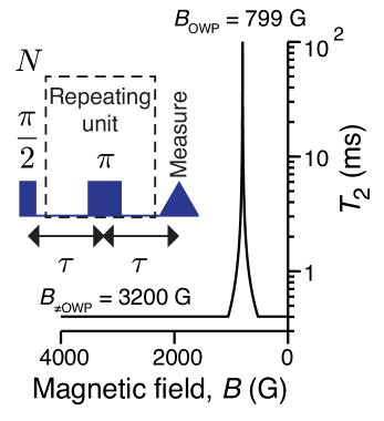
Figure 7.1: Illustrates coherence enhancement as $B\to B_{\textrm{OWP}}$ (the Hahn spin echo time $T^{(1)}_{2}$ is plotted). The OWP is for a bismuth donor in natural silicon, investigated experimentally in Wolfowicz et al. (2013) and Balian et al. (2014). The OWP curve was calculated using the analytical formula Equation (6.1). OWP results are for the $\left|{14}\right\rangle\to\left|{7}\right\rangle$ transition for which $B_{\textrm{OWP}}=799$ G. Inset: The CPMG dynamical decoupling sequence consists of the initial $\pi/2$ pulse, followed by the $-\tau-\pi-\tau-$echo sequence repeated $N$ times, as described in Section 2.2.3. Figure adapted from Balian et al. (2015).

7.4 Low and Moderate Pulsed CPMG

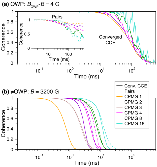
Figure 7.2: Shows dependence of the coherence on the number of dynamical decoupling pulses $N$, (a) near an optimal working point (OWP) and (b) far from an OWP, for modest numbers of $N$. (a) For $B$ close to $B_{\textrm{OWP}}$, the $T_{2}$ times show comparatively little response to dynamical decoupling. Further, even though the initial coherence is extended with increasing $N$, the decays become ever more oscillatory. For low $N$, the independent pairs contribution is largely eliminated. Inset of (a): Showing complete suppression of the independent pairs contribution near an OWP; but showing also its gradual revival as $N$ increases. (b) In contrast, far from the OWP, substantial (order of magnitude) enhancement of the $T_{2}$ time by dynamical decoupling is achieved with a moderate (preferably even) number of pulses. Decays for independent pair contributions (dashed lines, CCE2) and the converged quantum many-body numerics (solid lines, CCE4) are also compared, indicating that as $N\gtrsim 10$, once again, the independent pair contribution is sufficient. CCE calculations were performed for CPMG$N$ on a bismuth donor in natural silicon for $B$ along $[100]$ and for the $\left|{14}\right\rangle\to\left|{7}\right\rangle$ transition for which $B_{\text{OWP}}=799$ G. In (a), $B=795$ G while for (b), $B=3200$ G. The converged CCE in (a) corresponds to CCE3. Figure adapted from Balian et al. (2015).

Details of the CCE simulations are the same as described in Chapter 5, but for the CPMG sequence. The results shown are for the same single realisation of bath spin positions and the same initial product bath state. In this section we discuss CPMG$N$ with $N=1-16$ and present higher-order CPMG in a later section below.

The coherence decays for the Hahn spin echo ($N=1$) were presented in Chapter 5. In Figure 7.2, these are plotted together with CPMG for $N$ up to 16, both near (Figure 7.2(a)) and far (Figure 7.2(b)) from OWPs, the decays corresponding to converged CCE, and also pair correlations for the case close to OWPs (inset of Figure 7.2(a)). One notable feature of the comparison near and far from OWPs is the insensitivity of OWP behaviour to low numbers of pulses, in sharp contrast to the $\neq$OWP regime where there is a factor of 3 “jump” in $T_{2}$ from CPMG1 to CPMG2; while for larger $N$, we find $T_{2}\sim N$. However, OWPs are extremely effective at suppressing decoherence: for the point shown near the OWP, $T_{2}\simeq 100$ ms already at CPMG1, while away from the OWP, to obtain comparable values, $N\simeq 100$ pulses are required as will be shown later. Previous studies, including the recent study in Ma et al. (2014) of the ESR dynamics of a phosphorus donor at $X$-band frequencies (a system without OWPs for electron qubit decoherence and which is comparable to our $\neq$OWP regime), observed a sharp increase in the coherence time between CPMG1 and CPMG2. Analysis with the linked-cluster expansion method suggested that spin-pair contributions were fully suppressed (Ma et al., 2014). But we show CCE2 in $\neq$OWP regimes to still give a reasonable approximation to the magnitude of the observed $T_{2}$ time, for both CPMG1 and CPMG2. In the case away from an OWP, the FID is very similar to CPMG1. This is in contrast to the OWP, where CCE2 gives no decay at all, while the FID gave decay curves comparable to converged CCE3 (and Equation (6.1)). Thus, there is a drastic change from FID to CPMG1 at OWPs; in contrast, for regimes away from an OWP, there is little change between FID and CPMG1, but a strong enhancement for CPMG$N$ with $N>1$.

We find that three-spin clusters not only restore the CCE2 short-time decay, but in fact suffice to give results converged with respect to the many-body dynamics (i.e. there is little difference between CCE3 and CCE5) for both Hahn echo decays and modest $N\lesssim 20$ pulse numbers. For larger $N$, we find that CCE2 once again gives converged decays.

For any kind of spin diffusion, whereby the magnetic noise arises from flip-flopping (e.g. dipolar-coupled) spins in the bath (i.e. “indirect flip-flops”), the noise from non-interacting pairs of bath spins provides a reasonable estimate for the $T_{2}$ timescale of measured echo decays. For the case of isotopically-enriched samples, where donor-donor dynamics replaces the nuclear bath, larger spin clusters (CCE3 to CCE6) represent a quantitative correction (Witzel et al., 2010, 2012). In our case, unlike in Ma et al. (2014), CPMG$N$ with small $N$ eliminates pair dynamics in the sense that CCE2 (using only clusters of two bath spins) does not even give a finite $T_{2}$ time. Such complete suppression, and also in the absence of any higher order $N>1$ dynamical decoupling is quite exceptional.

The quantum numerics do evidence a clear dependence of the pair contribution on pulse number $N$. For example, in the inset of Figure 7.2(a), we have shown that, for a given field $B$ in the vicinity of the OWP, as $N$ increases to $N\simeq 16$, the pair contribution once again gives significant decay. To suppress decay for $N=16$ one must choose a value of $B$ even closer to the OWP. In fact this was one of our main findings: whether at OWPs or far from OWPs, our comparisons between many-body CCE3-5 and calculations involving only pairs show that increasing $N$ gradually restores the importance of the pair contribution, relative to $N=1$ or $N=2$, where many-body effects are seen to make the dominant contribution.

7.5 Pseudospin Analysis

We now proceed to analyse correlations from independent pairs in order to obtain insight on the effect of dynamical decoupling near and far from OWPs. We employ the well-established pseudospin model of the system-bath dynamics as was used for the single-spin FID in Chapter 6.

After preparing the initial qubit superposition, the CPMG$N$ pulse sequence can be summarized as $[\hat{T}(\tau)-\pi-\hat{T}(\tau)]^{N}$, with final evolution time $t=2N\tau$. The unitaries $\hat{T}(\tau)$ represents free evolution and $\pi$ denotes the refocusing pulse which flips between $\left|{u}\right\rangle$ and $\left|{l}\right\rangle$: $\left|{u}\right\rangle\left\langle{l}\right|+\left|{l}\right\rangle\left\langle{u}\right|$ but leaves all other central states and the bath unperturbed. Note that for the case of the numerical CCE calculations of any order (including central state depolarising terms), $\hat{T}(\tau)$ represents free evolution under the total Hamiltonian in Equation (2.6). For the case of pseudospins, the pure dephasing approximation must hold.

In the pair correlation approximation or CCE2, the coherence decay is simply given by

$$\mathcal{L}(t)=\prod_{k}|\mathcal{L}_{k}^{[N]}(t)|,$$ (7.1)

where $|\mathcal{L}_{k}^{[N]}|$ is the decay contribution from the $k$-th spin pair for CPMG$N$ and the product is over all spin pairs in the bath. The analysis below considers the individual pair decay envelopes $|\mathcal{L}_{k}^{[N]}|$ of which there are $\approx 10^{4}$ in the bath and we have dropped the label $k$ for clarity.

In order to evaluate the bath state overlap (Equation (2.18)) or equivalently the decoherence $\mathcal{L}^{[N]}(t)$ as described in Chapter 2, we must first evaluate

$$\left|{\mathcal{B}_{u,l}(t)}\right\rangle=\hat{T}^{[N]}_{u,l}\left|{\mathcal{B}(0)}\right\rangle,$$ (7.2)

where the unitaries $\hat{T}^{[N]}_{u,l}$ for CPMG$N$ are given by a product sequence of $\hat{T}^{[0]}_{u}$ and $\hat{T}^{[0]}_{l}$, which correspond to evolutions under the pseudospin Hamiltonians $\hat{h}_{u,l}$ (Equation (6.4)): $\hat{T}^{[0]}_{u,l}=\exp{[-i\hat{h}_{u,l}]}$. Refocusing pulses simply switch between $u$ and $l$ in applying the unitaries. For example, for the simple case of the Hahn spin echo (i.e. CPMG1), the unitaries are given by $\hat{T}^{[1]}_{u,l}=\hat{T}_{u,l}^{[0]}\hat{T}_{l,u}^{[0]}$ (note the order of $u$ and $l$).

We first diagonalise $\hat{h}_{u,l}$. We can now write, for the Hahn echo ($N=1$)

$$\hat{T}^{[1]}_{u,l}=A_{0}\hat{\mathds{1}}-i{\bf{A}}_{u,l}\cdot\hat{\bm{\sigma}},$$ (7.3)

where ${\bf A}_{u}=(A_{x},A_{y},A_{z})$ and $\hat{\bm{\sigma}}$ is the vector of Pauli matrices acting on the bath basis: $\{\left|{\downarrow\uparrow}\right\rangle,\left|{\uparrow\downarrow}\right\rangle\}$. The ${\bf A}_{u,l}$ components depend on time and can easily be given explicitly in terms of the pseudospin parameters (Lang et al., 2015):

$$A_{0}(\tau) =\cos(\omega_{u}\tau)\cos(\omega_{l}\tau)-\sin(\omega_{u}\tau)\sin(\omega_{l}\tau)\cos(\theta_{u}-\theta_{l}),$$

$$A_{x}(\tau) =\sin(\omega_{l}\tau)\cos(\omega_{u}\tau)\sin(\theta_{l})+\cos(\omega_{l}\tau)\sin(\omega_{u}\tau)\sin(\theta_{u}),$$

$$A_{y}(\tau) =-\sin(\omega_{u}\tau)\sin(\omega_{l}\tau)\sin(\theta_{u}-\theta_{l}),$$

$$A_{z}(\tau) =\sin(\omega_{l}\tau)\cos(\omega_{u}\tau)\cos(\theta_{l})+\cos(\omega_{l}\tau)\sin(\omega_{u}\tau)\cos(\theta_{u}),$$ (7.4)

where $\theta_{i}$ and $\omega_{i}$ are the pseudofield angles and pseudospin frequencies respectively (see Chapter 6 for details and the pseudospin Hamiltonian). The only term which is not invariant with respect to the exchange $u\leftrightarrow l$ is $A_{y}$ and thus ${\bf A}_{l}=(A_{x},-A_{y},A_{z})$.

The coherence envelope for each spin pair $|\mathcal{L}^{[N]}(t)|\propto|\langle\mathcal{B}(0)|\hat{T}^{\dagger[N]}_{l}\hat{T}^{[N]}_{u}|\mathcal{B}(0)\rangle|$ is obtained simply from $\hat{{L}}^{[N]}(t)\equiv\hat{T}^{\dagger[N]}_{l}\hat{T}^{[N]}_{u}$. For both CPMG1 and CPMG2, the unitarity of the evolution of upper relative to lower states is broken by a term proportional to $A_{y}$. For CPMG1,

$$\hat{L}^{[1]}(t)=\hat{\mathds{1}}-2iA_{y}\hat{\sigma}_{y}\hat{T}^{[1]}_{u}.$$ (7.5)

We can consider higher sequences; since $\hat{T}^{[2]}_{u}=\hat{T}^{[1]}_{u}\hat{T}^{[1]}_{l}$ and $\hat{T}^{[2]}_{l}=\hat{T}^{[1]}_{l}\hat{T}^{[1]}_{u}$, we obtain for CPMG2:

$$\hat{L}^{[2]}(t)=\hat{\mathds{1}}-4iA_{y}(A_{z}\hat{\sigma}_{x}-A_{x}\hat{\sigma}_{z})\hat{T}^{[2]}_{u}.$$ (7.6)

Both the above general expressions apply equally to either OWP or the $\neq$OWP regimes. The only important difference between these regimes is that $\theta_{u}\to\theta_{l}$ for the approach to an OWP and $\theta_{u}=\pi-\theta_{l}$ for the spin away from the OWP. Alternatively, from the explicit expressions for the components of ${\bf A}_{u,l}$, we see that the OWP condition is $A_{y}\to 0$; since $A_{y}$ is the prefactor to both the above expressions, CPMG1 and CPMG2 are equally suppressed at OWPs.

For the thermal initial bath states $\left|{\downarrow\uparrow}\right\rangle$ or $\left|{\downarrow\uparrow}\right\rangle$, the temporal coherence decay for the bath spin pair is $|\mathcal{L}^{[N]}(t)|=|\left\langle{\downarrow\uparrow}\right|\hat{L}^{[N]}(t)\left|{\downarrow\uparrow}\right\rangle|=|\left\langle{\uparrow\downarrow}\right|\hat{L}^{[N]}(t)\left|{\uparrow\downarrow}\right\rangle|$ (the states $\left|{\downarrow\downarrow}\right\rangle$ and $\left|{\uparrow\uparrow}\right\rangle$ are not involved in pure dephasing decoherence).

We can easily obtain the coherence decay envelopes for CPMG1 in general, assuming pulse interval $\tau$:

$$|\mathcal{L}^{[1]}(t=2\tau)|^{2}=1-4A_{y}^{2}A_{0}^{2},$$ (7.7)

emphasising that $A_{0}\equiv A_{0}(\tau)$, ${\bf A}_{u,l}\equiv{\bf A}_{u,l}(\tau)$. For arbitrary even numbers of pulses, CPMG$N$ such that $N/2$ is an integer,

$$\mathcal{L}^{[N]}(t=2N\tau)=1-\frac{2A_{y}^{2}}{A_{y}^{2}+A_{0}^{2}}\sin^{2}\left[\frac{N\phi(\tau)}{2}\right],$$ (7.8)

where $\cos\phi(\tau)=A_{0}(2\tau)$. An equivalent expression was obtained in Zhao et al. (2012a). Both expressions Equation (7.7) and Equation (7.8) are equally valid for both regimes (OWP and $\neq$OWP).

7.5.1 Near Optimal Working Points

The only important difference between these regimes is that $\theta_{u}\to\theta_{l}$ for the approach to an OWP and $\theta_{u}=\pi-\theta_{l}$ for the spin away from the OWP. Alternatively, from the explicit expressions for the components of ${\bf A}_{u,l}$, we see that the OWP condition is $|A_{y}|\to 0$. Thus, the suppression of qubit-bath correlations from pairs for OWPs is of the same order for CPMG1, CPMG2 or any other even-pulsed CPMG: for all bath spin pairs equally, the decay due to correlations from each independent pair uniformly tends to zero as $(A_{y})^{2}\to 0$ as $B\to B_{\textrm{OWP}}$.

The dependence on $N$ is entirely contained in the $\sin^{2}[N\phi(\tau)/2]$ term. If $N\phi(\tau)\ll 1$ then increasing $N$ has a strong amplifying effect on the signal, while if $N\phi(\tau)\gg 1$, increasing $N$ simply results in oscillatory behaviour. Near OWPs, from the expression for $A_{0}(2\tau)$, we see that if $\theta_{u}=\theta_{l}$, $\phi(\tau)/2\simeq(\omega_{u}+\omega_{l})\tau$. Hence we only expect a response to dynamical decoupling if $\tau$ is sufficiently small (i.e. if $\tau\lesssim(\omega_{u}+\omega_{l})^{-1}$).

7.5.2 Far from Optimal Working Points

In contrast, for CPMG away from an OWP, the $A_{y}^{2}$ prefactor is still there, but is not small. The origin of the suppression of correlations from independent pairs for small numbers of pulses is more subtle to analyse with the pseudospin model. For CPMG2 in the $\neq$OWP limit, we obtain

$$|\mathcal{L}^{[2]}(t)|^{2}=1-64A_{y}^{2}A_{0}^{2}A_{x}^{4}.$$ (7.9)

The large jump in $T_{2}$ from CPMG1 to CPMG2 was also analysed in Ma et al. (2014). In the notation of Ma et al. (2014), we see that for CPMG1, the decay envelope is of order $n_{x}^{2}$, while for CPMG2 it is of order $n_{x}^{6}n_{z}^{2}$, where $n_{x}=\sin{\theta_{u}}=\sin{\theta_{l}}$ while $n_{z}=\cos{\theta_{u}}=-\cos{\theta_{l}}$. Since the bath spans all angles $|\theta_{u,l}|=[0,\pi/2]$ one cannot a priori assume $\sin{\theta_{u,l}}$ is small. However, previous numerical studies support the idea that those spin pairs which have $|J_{1}-J_{2}|\gg|C_{12}|$ (i.e. are strongly coupled to the central system) and therefore small pseudospin angles, dominate the Hahn echo contribution (Balian et al., 2014) (see strong coupling approximation Chapter 6). For CPMG2, such strong-coupled spin pairs are strongly suppressed, and so $T_{2}$ becomes dominated by more weakly coupled spin pairs which are less effective in decohering the qubit.

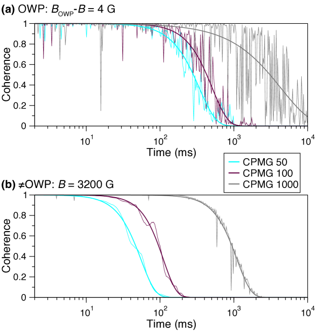
Figure 7.3: Shows coherence decays for large numbers ($N$) of dynamical decoupling pulses (a) near and (b) far from OWPs; as shown in the inset of Figure 7.2(a), for such high $N$, correlations from independent pairs once again dominate the decays in all regimes so CCE2 is converged and plotted. The behaviour at OWPs is now sensitive to $N$ but the decays here become increasingly oscillatory as $N$ and $T_{2}$ both become large; we attribute this to large numbers of bath spin-pair frequencies becoming resonant with the pulse spacing. It indicates the behaviour one might expect in a single-shot single spin study. The smooth lines are fits to the decays and indicate the expected coherence decay after ensemble averaging. CCE calculations were performed for a bismuth donor in natural silicon for $B$ along $[100]$ and $B_{\text{OWP}}=799$ G. Figure adapted from Balian et al. (2015).

7.6 High Order CPMG

We now investigate CPMG$N$, with $50\leq N\leq 1000$ pulses. For such large $N$, decays from independent pairs only (CCE2) are restored as well as the sensitivity to dynamical decoupling at OWPs. Even for $N=16$ (Figure 7.2) we see that the initial period of no decay $\mathcal{L}(t)\sim 1$ is prolonged. For larger $N$ (Figure 7.3), the enhancement of coherence even at OWPs is clear, but however, the decays become extremely noisy. The noise can be attributed to the timescales of individual nearby spin clusters and the time interval between pulses. For these long coherence times ($T_{2}\sim 1$ s) there are very large numbers of resonances. The CPMG sequence provides a means of amplifying noise from nearby clusters whenever pulse intervals become resonant with the characteristic cluster frequency. While this makes CPMG a valuable technique for spin detection (Zhao et al., 2012b), large numbers of such resonances are undesirable if the aim is to protect qubit coherence. In contrast, far from OWPs, the decays for high $N$ remain relatively smooth. While the noise at OWPs can be mitigated by ensemble averaging, this is likely to introduce a considerable disadvantage in terms of single-shot operation of a single hybrid qubit.

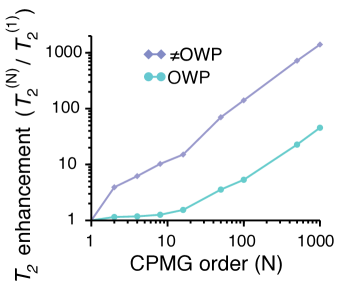
Figure 7.4: Effect of dynamical decoupling (CPMG with even pulse numbers $N$) as $N\to\infty$. Plots $T^{[N]}_{2}/T_{2}^{[1]}$ showing enhancement of the electron spin coherence time $T_{2}$ as a function of pulse number $N$, relative to the $N=1$ Hahn echo value. We find that while dynamical decoupling far from the OWP enhances $T_{2}$ by an order of magnitude with about 10 pulses, in contrast, close to an OWP, enhancement is marginal for dynamical decoupling with low $N$. For high $N$, enhancements near and far from OWPs become comparable. Even-pulsed CPMG is shown as it is more effective than CPMG with odd numbers of pulses. The coherence times are when the CPMG decays in Figure 7.2 and the fits to the decays in Figure 7.3 have fallen to $1/e$. Results are for Si:Bi in natural silicon for the $\left|{14}\right\rangle\to\left|{7}\right\rangle$ transition for which $B_{\textrm{OWP}}=799$ G. For the field value near the OWP ($B=795$ G), $T_{2}^{[1]}\simeq 96$ ms while $T_{2}^{[1]}\simeq 0.79$ ms in the $\neq$OWP regime ($B=3200$ G). Figure adapted from Balian et al. (2015).

7.7 Summary of Coherence Times

In sum, we have seen that a key difference between OWP and $\neq$OWP behaviours arises from the $A_{y}^{2}\propto\sin^{2}({\theta_{u}-\theta_{l}})$ prefactor which globally suppresses all independent pair contributions on the approach to an OWP, and accounts for the drastic effect at OWPs, but which is independent of $N$ and has little effect far from OWPs. However, to analyse decays resulting from dynamical decoupling one must consider the remainder of the expression in Equation (7.8), which reflects the dependence on $N$.

The ineffectiveness of dynamical decoupling near OWPs for small $N$ can also be understood with an intuitive picture considering the relevant timescales of the system. For dynamical decoupling to be effective, the time interval between pulses ($t/2N$) must be shorter than to the correlation time of the bath $\tau_{c}$. Since typical intra-bath interactions are at most a few kHz, $\tau_{c}\sim 1$ ms. Near the OWP, $\omega_{u}\simeq\omega_{l}$ and $\theta_{u}\simeq\theta_{l}$, so the frequency of the bath noise spectrum ($\sim\omega_{u,l}$) is appreciably higher than $1/\tau_{c}$ and thus dynamical decoupling becomes ineffective in extending the coherence time $T_{2}\gg\tau_{c}$. At short times and for high $N$ however ($t/2N<\tau_{C}$), dynamical decoupling does protect the central system as evidenced for CPMG16 in Figure 7.2(a) and higher $N$ in Figure 7.3. In contrast, dynamical decoupling is far more effective in extending $T_{2}$ away from the OWP and for relatively small $N$ (Figure 7.2(b)); although the pseudospin frequencies are comparable, the pseudospin fields are in opposing directions ($\theta_{u}\simeq\pi-\theta_{l}$), thus, the frequency of noise is much slower and becomes comparable to $1/\tau_{c}\sim 1/T_{2}$.

The enhancement of coherence times relative to the Hahn spin echo is shown for increasing $N$ in Figure 7.4. As an OWP is approached, dynamical decoupling gives little enhancement in $T_{2}$ with increasing $N$ for the first 100 or so pulses, in sharp contrast to regimes far from an OWP, where $T_{2}$ scales roughly as $N$ and there is a substantial enhancement already between $N=1$ and $N=2$.

7.8 Inhomogeneous Broadening

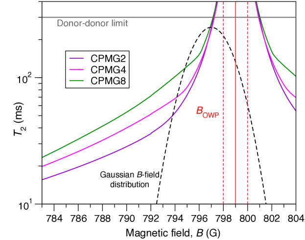
Figure 7.5: Sharp $B$-field dependence of $T_{2}$ for various CPMG orders near an OWP. Inhomogeneous broadening from ²⁹Si nuclei can be incorporated by convolving the decays with a Gaussian $B$-field distribution centred about $B$ (here centred about $797$ G) and with standard deviation $w\simeq 2$ G (dashed line). For a donor concentration of $3\times 10^{15}$ cm^-3, $T_{2}$ is limited by donor-donor processes at about $300$ ms (Wolfowicz et al., 2013). The $T_{2}$ lines were calculated for bismuth donors in natural silicon using the CCE up to 3rd order and for $B\parallel[\bar{1}10]$. The OWP under investigation is shown in red at $799$ G. Figure adapted from Balian et al. (2015).

Finally, it is important to note that for direct quantitative comparisons between our dynamical decoupling calculations and experimental ensemble measurements, inhomogeneous broadening due to ²⁹Si nuclei might also have to be factored in. This is because there is a sharp $B$ dependence of $T_{2}$ near an OWP over a narrow $B$ region.

The sharp variation of $T_{2}$ with $B$ over a few G near an OWP is shown in Figure 7.5 for various orders of CPMG. Inhomogeneous broadening of $B$ due to ²⁹Si impurities has a FWHM of about $4$ G in natural silicon. As described in Chapter 5 and Chapter 6, the broadening can be simulated by convolving the decays with a Gaussian $B$-field distribution according to Equation (5.4).

Depending on the donor concentration, donor-donor processes may also need to be included. For example, for a donor concentration of $3\times 10^{15}$ cm^-3, $T_{2}$ near an OWP is limited by direct flip-flops of the central donor with other donors in the ensemble (Wolfowicz et al., 2013). The measured $T_{2}$ in isotopically enriched samples ranges from $0.2-2$ s ($T_{2}$ for a donor concentration of $3\times 10^{15}$ cm^-3 is 300 ms). Therefore, care should be taken to include donor-donor processes very near the OWP (within about 1 G), where nuclear spin diffusion coherence times are comparable to those of donor-donor processes.

7.9 Conclusion

Understanding the interplay between OWPs and dynamical decoupling involves understanding of the quantum behaviour as a function of the two limits $B\to B_{\textrm{OWP}}$ and $N\to\infty$ corresponding to approaching an OWP and simultaneously increasing the number of dynamical decoupling pulses.

For the Hahn spin echo case (Chapter 5) and for low to moderate pulsed dynamical decoupling, pair correlations are drastically suppressed and 3-body CCE is essential for predicting and understanding decays near OWPs. Even away from OWPs, it was shown that many-body effects make an appreciable contribution for $N\lesssim 10$. However, once $N\to\infty$ there is little difference between pair correlation and higher-CCE results in all regimes.

For practical applications, one can hope to identify the best strategy for enhancing the coherence of donor qubits whilst still keeping the nuclear spin bath of naturally occurring silicon for its potential technological use. We note that the magnetic field in Figure 7.2(a) and Figure 7.3(a) is about 4 G from the actual OWP. Although in a theoretical calculation one can obtain a longer $T_{2}$ at a point closer to the OWP without dynamical decoupling, the ESR linewidth due to ²⁹Si impurities restricts the measured value at the OWP.

By operating near OWPs without dynamical decoupling, the maximum achievable $T_{2}$ is 0.1 s due to inhomogeneous broadening from the environmental nuclei (Wolfowicz et al., 2013; Balian et al., 2014). For isotopically enriched samples in which the nuclear spin bath is nearly eliminated, $T_{2}$ at the OWP was measured to be about 1 s and is limited by decoherence mechanisms involving donor-donor interactions (Wolfowicz et al., 2013). Therefore, to bridge this single order of magnitude difference in $T_{2}$ for an ensemble at OWPs without resorting to isotopic enrichment, dynamical decoupling should be applied with at least a few hundred pulses. The effect of dynamical decoupling in extending coherence times near an OWP is marginal with a moderate number of pulses (up to $N\sim 16$) in contrast to the usual regimes far from OWPs. For high donor concentrations, the timescale of donor-donor decoherence is comparable to the $T_{2}$ obtained in a nuclear spin bath, hence one might also want to investigate suppressing those mechanisms with dynamical decoupling.

However, combining dynamical decoupling with OWPs is not without its drawbacks. As $T_{2}$ and $N\to\infty$, individual few-spin clusters in a silicon bath may become resonant with the dynamical decoupling pulse spacing, resulting in very noisy decays in single central spin realisations. Although ensemble measurements are unaffected by this noise, this means that for single-qubit operations, if OWPs can be exploited, their extraordinary potential for coherence suppression (which has no noisy decay behaviour without dynamical decoupling) may be sufficient.

At the time of writing, Ma et al. (2015) (with experiments by Dr. Gary Wolfowicz and Professor John Morton) reported $T_{2}\simeq 1$ s near an OWP with 128 dynamical decoupling pulses in natural silicon. This is in broad agreement with our predictions as can be seen in Figure 7.3 where we predict $T_{2}\simeq 0.5$ s with 100 pulses with $B$ shifted by 4 G from the OWP; the measurements were made 1.5 G from the OWP and for 28 more pulses (Ma et al., 2015).

8  |  Decoherence of Nuclear Spins
Proximate to Hybrid Qubit

The content of this chapter differs from the rest in that the decoherence dynamics studied is for nuclear spins; specifically, for a ²⁹Si spin-1/2 (Guichard et al., 2015). Hyperfine couplings of proximate ²⁹Si sites in an ensemble have been spectroscopically resolved by CW ENDOR (Hale and Mieher, 1969a, b) and also pulsed ENDOR techniques (Morton et al., 2008; Balian et al., 2012; Wolfowicz et al., 2015b) as described in Chapter 4. The pulsed experiments in Chapter 4 demonstrate the feasibility of quantum control of such ²⁹Si spins. Their coherence may also be investigated by pulsed ENDOR. As mentioned in Chapter 1, the Hahn echo coherence time for a ²⁹Si qubit in a spin bath formed of other ²⁹Si spins is about 5 ms (Dementyev et al., 2003). Recently, Pla et al. (2014) measured $T_{2}$ of a single ²⁹Si spin to be 6.4 ms, close to the measured bulk value reported in Dementyev et al. (2003).

Here, we investigate the situation of a nucleus in close proximity to the hybrid qubit (or proximate nuclear spin). We show that in this case, coherence times can reach the second timescale (Guichard et al., 2015), in agreement with ensemble measurements (Wolfowicz et al., 2015b). Thus, the hybrid qubit in a sense enhances the coherence of proximate nuclear spins. In this scenario, one can imagine a long-lived quantum register (memory) implemented as the nuclear spin, while processing is carried out on the donor qubit. As of now, there is no $T_{2}$ measurement of a single proximate nuclear spin in the presence of the donor. This parameter is of interest to potential future realisations using nuclear spin registers in combination with electronic qubits in silicon, analogous to the situation involving NV centres and ¹³C nuclei in diamond (Cappellaro et al., 2009; Waldherr et al., 2014; Taminiau et al., 2014).

The theoretical work in this chapter was motivated by experiments measuring coherence times of proximate nuclear spins by Dr. Gary Wolfowicz, Dr. Pierre Mortemousque and Professor John Morton. The measurements were performed on Si:P in the high-field limit. Hence, the hybrid qubit we study here is in the unmixed ESR limit, implemented as Si:P which is equivalent to Si:Bi in the limit $B\to\infty$ for our purposes; i.e. a simple electronic spin-1/2. The theoretical analysis was published in Guichard et al. (2015) and the experimental measurements were very recently reported in Wolfowicz et al. (2015b).

In short, we investigate the decoherence mechanism of a proximate nuclear impurity spin in the quantum bath formed of other impurity spins. We propose two models of decoherence which give coherence times on the same timescale. Both are spin diffusion models, analogous to the case of decoherence for the hybrid qubit discussed in Chapter 5, Chapter 6 and Chapter 7; however, they differ from usual spin diffusion problems in terms of the properties of clusters which dominate the decoherence dynamics. The first is a very large nuclear spin bath far from the nuclear qubit, comprising $\gtrsim 10^{8}$ weakly contributing spin pairs. The second involves decoherence driven by pairs of symmetrically sited nuclear spin pairs, due to symmetries of the donor electron wavefunction. There are only of order $10^{2}$ such “equivalent pairs”. In previous studies (i.e. for decoherence of donor spins or non-proximate nuclear spins), both models produce negligible contributions to coherence decays as will be explained below. Both models give $T_{2}$ times of order 1 s in agreement with measured proximate nuclear spin coherence times, confirming the suitability of proximate nuclei in silicon as very long-lived spin qubits. We also note that if equivalent pairs represent a measurable source of decoherence, nuclear coherence decays could provide sensitive probes of the symmetries of electronic wavefunctions.

8.1 The Frozen Core

Figure 8.1: Decoherence of electronic spin qubits (or equivalently hybrid qubit in the unmixed limit with the two levels separated by ESR frequencies) by a flip-flopping nuclear spin bath in natural silicon. The background plots the spatial electronic wavefunction; blue denotes the strong-detuning region, where the energy cost of a bath spin flip $\Delta_{e}^{\pm}\propto\pm(J_{1}-J_{2})$ exceeds the strongest intra-bath coupling $C_{12}$; it thus corresponds to the usual definition of the “frozen-core” region. However, electronic spin decoherence is dominated by an active zone (purple colour) of pairs of nuclear spins which are actually within the blue strongly detuned region, with $|\Delta_{e}^{\pm}/C_{12}|=|(J_{1}-J_{2})/C_{12}|\sim 10$ for Si:P (see Chapter 6 for details). The reason is that, while for large $|\Delta_{e}^{\pm}|$ flip-flop amplitudes are strongly damped, qubit state-dependence of the quantum bath evolution, essential for the entanglement between the electronic spin and bath which produces decoherence, is also proportional to $\Delta_{e}^{\pm}$. Spin pairs for which $J_{1}=J_{2}$ (equivalent pairs) have no effect on electronic decoherence and were not considered in previous studies. Figure adapted from Guichard et al. (2015).

Proximate spins lie within a so-called “frozen core” region, where the donor electronic hyperfine interaction strongly suppresses nuclear dynamics. This is partly the reason for the lack of understanding of the decoherence dynamics of proximate nuclear spins in silicon. A pair of proximate nuclear spins can interact not only via direct dipolar coupling (Section 2.4.2), but also via the long-range interaction mediated by the central donor electronic spin (Section 2.4.4). In both cases, the two spins may flip-flop and this results in decoherence of either an electronic or nuclear qubit, whichever is coupled to the flip-flopping pair. However, in the case of strong hyperfine coupling between the nuclear impurity pair and the electron spin, the resulting energy detuning on each of the two members of the pair overwhelms the dipolar coupling, suppressing the flip-flop dynamics and in turn suppressing decoherence within the frozen core region.

The idea of the frozen core is well-established in the ESR community (Khutsishvili, 1967; Wald et al., 1992; George et al., 2010), but more recently there has been interest in utilizing it as a reservoir of protected qubits (Mildren and Rabeau, 2013) for the reasons outlined above. Therefore, it is of interest to determine coherence times of proximate nuclear spins in the frozen core. The boundary radius $R_{\text{FC}}$ of the frozen core is commonly set as the distance at which hyperfine coupling strengths have decreased to values comparable to the dipolar interactions between neighbouring nuclear spins (Mildren and Rabeau, 2013). Representative values of the latter may be inferred from measured linewidths; for example, the $127$ Hz linewidth of ²⁹Si in natural silicon (Hayashi et al., 2008) corresponds to an estimated $R_{\text{FC}}\approx 80$ Å for Si:P. As mentioned above, coherence times of proximate nuclear spins far outside the frozen core, are a few ms.

The argument that large energy detunings in the frozen core drastically suppress nuclear dynamics is not new. However, spin bath decoherence in terms of entanglement between the qubit (whether electronic or nuclear) and the environment has not been previously investigated in the frozen core. Before discussing nuclear-qubit spin decoherence, it is useful to summarise decoherence of the hybrid qubit with reference to the frozen core, in terms of detuned flip-flop nuclear bath dynamics – Figure 8.1 (see Chapter 5 and Chapter 6 for a comprehensive account). The large detunings in the frozen core lead to clear differences between decoherence of hybrid (or electronic) and proximate qubits, even when in both cases the same nuclear bath drives decoherence. Below, we take a more careful look at what is meant by the frozen core and where, precisely, its boundaries lie. For example, for the electronic qubits, decoherence is in fact dominated by impurities which lie within the usual definition of the frozen core as was shown in Balian et al. (2014) (see Chapter 6 for details), and as illustrated in Figure 8.1, since the detuning fully contributes to qubit-bath entanglement. Decoherence of proximate qubits, discussed in detail for the rest of this chapter, is summarised in Figure 8.2 and Figure 8.4.

8.2 Decoherence Dynamics of Nuclear Qubits

The two models we consider for proximate qubit decoherence in silicon arise from the usual pairwise flip-flops of nuclear impurities, but under extreme conditions, not encountered in previous decoherence studies such as that presented in Chapter 5 and Chapter 6.

As described in Chapter 2 and Chapter 5, it is not necessary to include all combinatorially allowed spin clusters; within $350$ Å of the donor site, there are in total $\sim 10^{10}$ ²⁹Si spin pairs. The smaller fraction of significantly contributing clusters are found by numerical search of each randomly populated lattice realisation by restricting the selection to, for instance, pairs within a certain distance and hyperfine coupling strength as explained in Chapter 2. However, inside the frozen core, applying the normal distance (or coupling strengths) thresholds turned out to be unreliable. Also, there is a drastic difference between the choice of spin clusters which must be included in the quantum bath for each of our two models; a few dozen for the equivalent pairs model, $\sim 10^{8}$ for the far bath model.

Regardless of the choice of spin clusters, the basic decoherence dynamics of proximate qubits is of the same physical origin as for the hybrid qubit in the unmixed limit – pairwise flip-flops are predominately responsible for dephasing. The process is equivalent to the usual CCE2 (pair correlations) but with detuning from the donor electron spin. Before proceeding, we note that since the central and bath spins are of the same species and higher correlations arising from larger clusters may be required for high accuracy (Witzel et al., 2010, 2012), but in both our models would represent only a minor quantitative correction, unlike the case encountered for the hybrid qubits near OWPs, where there was complete suppression of the pair correlation (as seen in Chapter 5). We summarise the basic decoherence mechanism of spin diffusion below, but including the suppressive effect of state-independent detuning provided by the electron spin, and emphasising the importance of state-dependent detuning which drives decoherence.

For the nuclear qubit ($I=1/2$), we use the notation $\left|{\pm}\right\rangle$ to represent the upper (spin-up; $+$) and lower (spin-down; $-$) states. The initial state after a $\pi$-pulse is

$$\left|\psi(t=0)\right\rangle=\frac{1}{\sqrt{2}}\left(\left|+\right\rangle+\left|-\right\rangle\right)\otimes\left|\mathcal{B}(0)\right\rangle\otimes\left|\phi(0)\right\rangle$$ (8.1)

where $\left|\phi(0)\right\rangle$ denotes the initial spin state of the effective donor electronic spin-1/2 which is not resonant with the external control pulses.

8.2.1 Spin Hamiltonian

The central spin Hamiltonian is simply a sum of Zeeman terms

$$\hat{H}_{\text{CS}}=\gamma_{e}B\hat{S}^{z}+\gamma_{n}B\hat{I}^{z}_{A},$$ (8.2)

where the qubit is labelled $A$ and the high-field limit is assumed for the coupled electron-nuclear donor at an ESR-type transition (i.e. no host donor nuclear spin terms). Written for a pair of nuclear bath spins labelled by $\hat{\bf I}_{l}$ ($l=1,2$), the interaction Hamiltonian is

$$\hat{H}_{\textrm{int}}=\sum_{l=1,2}\left(\hat{\bf S}\cdot\mathcal{J}_{l}+\hat{\bf I}_{A}\cdot\mathcal{D}_{l}\right)\cdot\hat{\bf I}_{l},$$ (8.3)

whereby the qubit is coupled to the electron spin via the hyperfine interaction ($\mathcal{J}$; Equation (2.35)) and to the bath spins via the dipolar interaction ($\mathcal{D}$; Equation (2.29)), which we take to be of secular form (Equation (2.31)). Because of the high-field limit and the large mismatch between electronic and nuclear gyromagnetic ratios, the hyperfine interaction can be approximated to include only Ising terms as given in Equation (2.36), with the residual electron-nuclear dipolar interaction becoming effective farther than about 20 Å from the donor site for Si:P. The long-range effect of non-Ising terms in the hyperfine interaction (RKKY; Section 2.4.4) are added as a correction to the intra-bath dipolar interaction as described in the following subsection below. Note that for simplicity, we do not include explicitly the hyperfine term coupling the electron to the resonant nuclear qubit $A$ ($J_{A}$), which is only significant in the specific (but minor) contribution from direct flip-flopping processes.

Finally, the bath Hamiltonian is given by a sum of two nuclear Zeeman terms and the secular dipolar interaction (Equation (2.31)):

$$\hat{H}_{\text{bath}}=\gamma_{n}B(\hat{I}^{z}_{1}+\hat{I}^{z}_{2})+C_{12}\hat{I}^{z}_{1}\hat{I}_{2}^{z}-\frac{C_{12}}{4}(\hat{I}^{+}_{1}\hat{I}_{2}^{-}+\hat{I}^{-}_{1}\hat{I}_{2}^{+}).$$ (8.4)

8.2.2 Nuclear Pseudospins

Under the action of the total Hamiltonian, the initial product state in Equation (8.1) evolves into an entangled state:

$$\left|{\psi(t)}\right\rangle=\frac{1}{\sqrt{2}}\left(\left[\left|{+}\right\rangle\otimes\left|{\mathcal{B}_{+}(t)}\right\rangle+\left|{-}\right\rangle\otimes\left|{\mathcal{B}_{-}(t)}\right\rangle\right]\otimes\left|{\phi(t)}\right\rangle\right),$$ (8.5)

where we have omitted the central-state phases as we take the modulus of the coherence below. As before, the coherence is given by the bath state overlap $|\mathcal{L}(t)|\propto|\left\langle{\mathcal{B}_{+}(t)}|{\mathcal{B}_{-}(t)}\right\rangle|$ and in the pair correlation approximation $\mathcal{L}(t)=\prod_{n}\mathcal{L}^{(n)}(t)$, where $\mathcal{L}^{(n)}(t)$ is the contribution from the $n$-th spin pair. To apply the pseudospin model as was done in earlier chapters, the pure dephasing approximation is required (perturbative corrections due to state depolarisation are possible to implement later in the formulation). We have already assumed an Ising form for the hyperfine interaction. As for the dipolar interaction of the qubit $A$ to the bath spins, we numerically find that the non-Ising terms (direct flip-flops) give negligible contribution to decoherence for both models. Neglecting such terms, the pseudpospin Hamiltonians for the nuclear qubit in a bath of two flip-flopping nuclei are written

$$\hat{h}_{\pm}=\frac{1}{4}(\Delta^{\pm}\hat{\sigma}_{z}+C_{12}\hat{\sigma}_{x})$$ (8.6)

where we have omitted the identity term which does not contribute to pseudospin coherence decays. The Pauli operators act on the basis $\{\left|{\downarrow\uparrow}\right\rangle,\left|{\uparrow\downarrow}\right\rangle\}$ of the two-spin-1/2 bath.

Crucially, the detuning is $\Delta^{\pm}=\Delta_{e}\pm(C_{1A}-C_{2A})$ for the proximate nuclear qubit, where $C_{1A}$ and $C_{2A}$ are the dipolar coupling strengths between each bath nucleus and the qubit. In this case, the electronic detuning $\Delta_{e}\equiv|J_{1}-J_{2}|$ represents a potentially large contribution which is not sensitive to the qubit state. For the Hahn echo case the coherence decay is given by:

$$|\mathcal{L}^{(n)}(t)|\simeq\left|1-2\alpha^{(n)}(\alpha^{(n)}+i\beta^{(n)})\right|,$$ (8.7)

where

$$\alpha =\sin(\omega_{+}t)\sin(\omega_{-}t)\sin{(\theta_{+}-\theta_{-})},$$

$$\beta =\sin(\omega_{+}t)\cos(\omega_{-}t)\sin\theta_{+}+\sin(\omega_{-}t)\cos(\omega_{+}t)\sin\theta_{-},$$ (8.8)

while $\theta_{\pm}=\tan^{-1}\left(C_{12}/\Delta^{\pm}\right)$, the eigenvalues $\omega_{\pm}=\dfrac{1}{4}\sqrt{(\Delta^{\pm})^{2}+(C_{12})^{2}}$, and we have dropped the pair label $n$ for convenience. The larger $\theta_{\pm}$, the larger the amplitudes of the flip-flopping of nuclear spin-pairs which drives the decoherence.

When considering the contribution of flip-flopping pairs that are within the frozen core, we obtained excellent agreement between the pseudospin equations above and numerical CCE2 provided that the well-known perturbative correction for the non-Ising hyperfine terms, i.e. the RKKY interaction (Section 2.4.4), was added to the dipolar coupling when using Equation (8.7). The RKKY interaction was included by adding to $C_{12}$ the term $(J_{1}J_{2})/{\gamma_{e}B}$. Note that for a numerical CCE calculation, the long-ranged interaction emerges naturally if the hyperfine interaction with non-Ising terms is included and the above-mentioned correction should not be applied.

For pairs in the frozen core with different hyperfine couplings to the electron spin, $|\Delta^{\pm}|\simeq\Delta_{e}\gg|C_{12}|$, thus $\theta_{\pm}\simeq 0$ and flip-flops become too strongly suppressed. The qubit state sensitivity enters in Equation (8.7) mainly via the $\sin{(\theta_{+}-\theta_{-})}$ prefactor and is also suppressed by $\Delta_{e}$. This imposes the further condition $|\Delta^{\pm}_{n}|=|(C_{1}^{A}-C_{2}^{A})|\gtrsim\Delta_{e}$ for a single individual pair to contribute appreciably to the decay. Central to our modelling is the identification of spin clusters within the frozen core which can contribute non-negligibly to the decoherence of a proximate spin. We now consider two models and apply them to the particular case of natural Si:P.

8.3 Far Bath Model

Figure 8.2: Decoherence of a proximate nuclear spin qubit (labelled “A”) by a quantum bath of nuclear spin pairs outside the frozen core. In contrast to electron spin decoherence (for which the detuning is fully state-dependent, see Figure 8.1), the detuning is now $\Delta_{e}+\Delta_{n}^{\pm}$: there is now potentially a very large state-independent component $\Delta_{e}\propto(J_{1}-J_{2})$ which simply damps the bath noise, in addition to a state-dependent component $\Delta_{n}^{\pm}\propto\pm(C_{1A}-C_{2A})$ which leads to qubit-bath entanglement and thus decoherence. For large $R$ (distance from donor site), the bath spin interaction with both the electron spin and nuclear qubit is dipolar, thus $|\Delta_{n}^{\pm}/\Delta_{e}|\sim 10^{-4}$ so very weak contributions from an extremely large bath of $10^{8}$ pairs for $50\lesssim R\lesssim 350$ Å must be combined to obtain a converged decay. Figure adapted from Guichard et al. (2015).

In this far bath model, we consider the decoherence from distant nuclear spin pairs, which are outside the frozen core and thus can flip-flop appreciably. We show that the typical contribution is so weak that we must include of order $10^{8}$ flip-flopping pairs outside the frozen core, at distances $R=50-350$ Å from the donor site, in order to obtain results converged with respect to bath size. In contrast, typical quantum-bath calculations of electronic spin decoherence require $\sim 10^{3}-10^{4}$ pairs to obtain convergence. The far bath model is illustrated in Figure 8.2.

From numerical simulations with a very large spin bath, we find that distant spin pairs outside the frozen core radius $R_{\textrm{FC}}$ individually make an extremely small contribution to decoherence: the $\alpha\propto\sin{(\theta_{+}-\theta_{-})}$ prefactor scales the coherence decays in Equation (8.7), since $|\mathcal{L}(t)|\sim 1-\alpha^{2}(\dots)$. We can also show that the approximate weight of the $n$-th pair, is of order $(1/T_{2}^{(n)})^{2}\propto\sin^{2}{(\theta^{(n)}_{+}-\theta^{(n)}_{-})}$ (Balian et al., 2014) (similar to the FID case in Chapter 6), assuming also the temporal character of the associated magnetic noise is relevant: in other words, flip-flop frequencies $\omega_{\pm}$ for the given pair cannot be orders of magnitude different from $\sim 1/T_{2}$. For a non-negligible contribution we would expect that $N_{p}\sin^{2}{(\theta_{+}-\theta_{-})}\sim 1$ where $N_{p}$ is a representative number of contributing spin pairs.

8.3.1 Convergence

Before presenting numerical convergence tests, we first give a heuristic argument in order to establish the size of the convergent far bath. From the pseudospin model (leaving out the $n$ labels),

$$\sin{(\theta_{+}-\theta_{-})}\simeq\frac{2C_{12}}{\omega}\ \frac{C_{1A}-C_{2A}}{\omega},$$ (8.9)

since $\omega_{\pm}\simeq\omega=\tfrac{1}{4}\sqrt{\Delta_{e}^{2}+C_{12}^{2}}$. Above, the factor $2C_{12}/\omega$ determines whether the pair can flip-flop appreciably and is significant if $|C_{12}/\Delta_{e}|\sim 1$. The second factor, $(C_{1A}-C_{2A})/\omega$ determines state distinguishability. For the far spins, the hyperfine mediated correction plays little role since $J_{1}$ and $J_{2}$ are small. For distances $R\gtrsim 100$ Å, where the Fermi contact component of the hyperfine interaction becomes small, the residual dipolar hyperfine interaction still makes a contribution to the detuning which is much larger than $(C_{1A}-C_{2A})$. Here,

$$\frac{(C_{1A}-C_{2A})}{\omega}\sim\frac{(C_{1A}-C_{2A})}{J_{1}-J_{2}}\sim\frac{\gamma_{n}}{\gamma_{e}}\simeq 10^{-4}.$$ (8.10)

Thus, the contribution of each such far bath spin pair is $\left(\tfrac{\gamma_{n}}{\gamma_{e}}\right)^{2}\sim 10^{-8}$, so only a far bath with $N_{p}\sim 10^{8}$ contributing spin pairs can produce significant decay. At very large $R$, however, $(C_{1A}-C_{2A})/\omega\to(C_{1A}-C_{2A})/C_{12}$ . But there is a minimum value of the interaction $C_{12}\equiv C^{\text{min}}_{12}$ where $(C^{\text{min}}_{12})^{-1}$ sets a timescale below which the bath noise is too slow to contribute. As $R\to\infty$, then $(C_{1A}-C_{2A})/C^{\text{min}}_{12}\to 0$, so there is a maximum radius $R_{\text{max}}$ beyond which the far bath does not contribute significantly to decoherence.

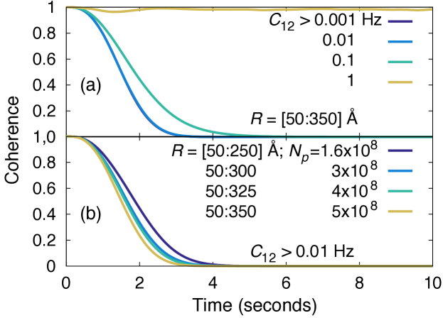
Figure 8.3: Convergence of large bath model with respect to intra-bath dipolar coupling (a) and with respect to bath size (b). The figure indicates that decoherence is dominated by spins with $C_{12}\sim 0.01-1$ Hz and a bath of spins within $R\lesssim 350$ Å  of the origin, combining the contributions from $5\times 10^{8}$ spin pairs. Calculations were performed for the case of Si:P, for $X$-band and magnetic field orientation $B_{0}=[100]$, yielding a $T_{2n}$ of 2 s for a single nuclear ²⁹Si spin sited at the origin. This represents an estimate for the upper bound for the coherence time if the far bath is the dominant process. Due to the large nuclear spin bath, the coherence decays are insensitive to the choice of random spatial realisation of the bath. Figure adapted from Guichard et al. (2015).

The analysis above was tested numerically by means of CCE2 calculations using a very large bath of nuclear spin pairs (excluding contributions from the second model we present below) and testing the effect on coherence decays of increasing the size of the bath. Figure 8.3 shows convergence with respect to bath size for Hahn echo decays, for a nuclear spin at the origin (thus expected to give an upper bound on the coherence). The $C_{12}\equiv C^{\text{min}}_{12}\sim 0.01-0.1$ Hz bound indicates that the pairs are within $40-50$ Å of each other and the calculation is converged with respect to bath size if we include $5\times 10^{8}$ spin pairs within $R_{\text{max}}\lesssim 350$ Å of the origin. The scale of the bath is remarkable, in comparison with comparable electronic spin or hybrid qubit decoherence calculations with $\sim 10^{4}$ pairs.

Although it is computationally feasible to solve for a bath of this magnitude by CCE2 or analytical pseudospin methods, the uniformity of the bath means that it is reliable to evaluate $\mathcal{L}$ in a smaller but geometrically representative sample of the bath. In addition, no averaging over bath realisations (bath spin positions) was required; the results are insensitive to whether one has a single spin or an ensemble.

Figure 8.4: Decoherence of a proximate nuclear spin qubit (labelled “A”) by a quantum bath of nuclear spin pairs inside the frozen core. See also Figure 8.2 for a comparison with decoherence outside the frozen core. The detuning on flip-flopping bath pairs is $\Delta_{e}+\Delta_{n}^{\pm}$; i.e., a sum of a potentially very large state-independent component $\Delta_{e}\propto(J_{1}-J_{2})$, which damps decoherence in addition to a state-dependent one $\Delta_{n}^{\pm}\propto\pm(C_{1A}-C_{2A})$ which drives decoherence. In the frozen core there are comparatively few spin impurities. For equivalent pairs however, $J_{1}=J_{2}\equiv J$ so $\Delta_{e}\simeq 0$. Their density is determined by the symmetry of the electronic wavefunction. The requirement for strong state-selective detuning implies also that one member of the pair must be close enough to the qubit to allow appreciable direct dipolar coupling (as opposed to long-range coupling between nuclear spins mediated by the electron spin). Pairs which also satisfy this requirement (exemplified by the upper, but not the lower, equivalent pair) are rare but even a few dozen suffice to exceed the contribution of the $\sim 10^{8}$ far-bath spin pairs shown in Figure 8.2. Figure adapted from Guichard et al. (2015).

8.4 Equivalent Pairs Model

In our second “equivalent pairs” (EP) model, the dephasing noise arises from a few dozen nuclear spin pairs, well within the frozen core, for which:

1. The members of the pair are symmetrically sited relative to the central spin and thus have equivalent values of the hyperfine detuning.

2. At least one member is sufficiently close to the nuclear qubit to have a significant dipolar interaction, while the other can be remote. The nuclear spins interact via the long-ranged hyperfine interaction mediated by the electron.

The indirect flip-flopping of these EPs is found to be most significant, but we include also the rarer contribution of direct flip-flops between the nuclear central spin and any equivalent partner it might have. We obtain $T_{2}$ values in the seconds timescale both for individual realisations (relevant to single donor experiments) and also for ensemble averages over many realisations. The EP model is illustrated in Figure 8.4.

8.4.1 Counting Equivalent Sites

The isotropic part of the hyperfine interaction is modeled using the Kohn-Luttinger wavefunction as described in Section 2.4.3. For phosphorus donors, the ionization energy is $0.044$ eV (Table 3.1). We can estimate the local densities of suitable EPs in the isotropic case before considering effects from any anisotropies in the hyperfine coupling arising from the residual electron-nuclear dipolar coupling.

In our simulations, the full lattice size ranges over $[-N,N]$ cubic cells of diamond cubic for each dimension, resulting in $8N^{3}$ unit cells and hence $64N^{3}$ total atomic sites (see Appendix C for details of the diamond cubic crystal structure). Equivalent sites are those with the same hyperfine interaction obtained using the Kohn-Luttinger wavefunction. We begin by considering the allowed coordinates of the impurities in the crystal. Owing to the symmetry of the system, each site possesses several potential equivalent partners, for which positions can be deduced from any allowed permutations of $(\pm n_{1},\pm n_{2},\pm n_{3})$ and which lie on the surface of shells of radius $R=\frac{a_{0}}{4}\sqrt{n_{1}^{2}+n_{2}^{2}+n_{3}^{2}}$, where ${\bf n}=(n_{1},n_{2},n_{3})$ is the integer vector for an atomic site and $a_{0}$ is the cubic lattice parameter. By consideration of the symmetries of the wavefunction, we can assign each vector $\bf{n}$ to a shell $s$ comprising $n_{s}=$ 48, 24, 12, 8, 6 or 4 partners and we first obtain $\mathcal{N}_{n_{s}}(N)$, the number of shells comprising $n_{s}$ partners within a radius of $R=Na_{0}$ from the center.

The ranges are adjusted to ensure summation over complete shells as follows. First, we divide site vectors into three classes as shown in Table 8.1. Summations must range between $[-N,N]$ for the 2 coordinates and $[-N,N-1]$ for the 0 coordinate of class 1 sites giving $4N^{2}(2N+1)$ number of sites; between $[-N,N]$ for class 2 giving $(2N+1)^{3}$ number of sites; and finally between $[-N,N-1]$ for class 3 giving $8N^{3}$ number of sites.

Class 1	Class 2	Class 3
(0,2,2)	(0,0,0)	(3,3,3)
(2,0,2)		(3,1,1)
(2,2,0)		(1,3,1)
		(1,1,3)

Table 8.1: The 8-site basis of the diamond cubic crystal structure (Appendix C) grouped into three classes. Class $X$ site vectors are obtained by modulo 4 translations of class $X$ basis vectors.

For each class, the contribution to a shell comprising $n_{s}$ partners within a radius of $R=Na_{0}$ of the center as a function of $N$ is summarized in Table 8.2. Additionally, class 2 contributes as $8N$ to $n_{s}=8$ and as $6N$ to $n_{s}=6$ and class 3 contributes as $8N$ to $n_{s}=4$.

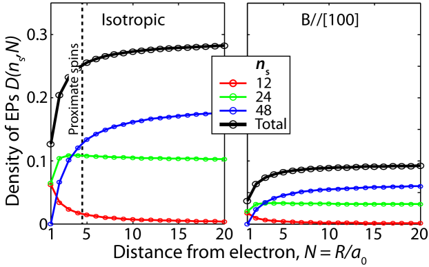
Figure 8.5: Density of equivalent pairs (EPs) as a function of distance from the donor site. The separate contributions from different types of shells is shown, as well as the total density, assuming a purely isotropic contact interaction (left) or a correction for anisotropic behaviour (right). The density of EPs is approximately constant for $R\gtrsim 10$ Å, but the innermost proximate spins typically interact with fewer EPs. Figure adapted from Guichard et al. (2015).

$n_{s}$	48	24	12
Class
1	$24N^{2}(N-1)$	$12N(3N-1)$	$12N$
2	$8N(N-1)(N-2)$	$36N(N-1)$	$12N$
3	–	$16N(N-1)(2N-1)$	$24N(2N-1)$

Table 8.2: Class contribution to the equivalent sites group as a function of $N$. Table adapted from Guichard et al. (2015).

We can now obtain estimates for $\mathcal{N}_{n_{s}}(N)$:

$$\mathcal{N}_{12}(N) = 4N^{2}$$

$$\mathcal{N}_{24}(N) = \frac{4}{3}N(N^{2}-1)+N^{2},$$

$$\mathcal{N}_{48}(N) = \frac{2}{3}N^{3}-N^{2}+\frac{N}{3},$$ (8.11)

while $\mathcal{N}_{8}(N)=\mathcal{N}_{6}(N)=N,\mathcal{N}_{4}(N)=2N$. Then assuming a binomial distribution, taking an abundance of $p=0.0467$ for nuclear spin impurities in natural silicon, the estimated average number of significant EP in each shell is:

$$\overline{\zeta}_{n_{s}}\simeq\sum_{k}\binom{n_{s}}{k}p^{k}(1-p)^{n_{s}-k}\ \frac{k(k-1)}{2},$$ (8.12)

where $\binom{n}{k}=\frac{n!}{k!(n-k)!}$ is the binomial coefficient. For the two dominant shells $\overline{\zeta}_{48}\sim 2.3$ and $\overline{\zeta}_{24}\simeq 0.6$. In these cases, it is quite likely that any impurity spin has an equivalent partner somewhere, albeit remotely located. Nevertheless, due to the long-range electron-mediated coupling, a $C_{12}$ of about tens of Hz is present. Within a sphere of radius $N$ cubic cells, we expect the total number of EP to be simply:

$$\mathcal{N}_{\textrm{EP}}\simeq\sum_{s}\overline{\zeta}_{n_{s}}\mathcal{N}_{n_{s}}(N).$$ (8.13)

For instance, within a radius of $R=100$ Å, we find $\mathcal{N}_{\textrm{EP}}\simeq 19,000$. For a proximate nucleus however, one member of the pair must be dipolar-coupled to the resonant spin (see caption of Figure 8.4) which is relevant within about $m\sim 3$ cubic cells. Each nuclear qubit thus interacts with other nuclei in the neighbouring $(2m)^{3}\sim 200$ cells. We can define a density of spin pairs:

$$D(n_{s},N=R/a_{0})=\frac{\overline{\zeta}_{n_{s}}\mathcal{N}_{n_{s}}(N)}{(2N)^{3}},$$ (8.14)

which gives the mean number of EPs in each cubic cell as a function of distance, $R=Na_{0}$ from the electron. We see in Figure 8.5 (left panel) that the mean number for large $R$ is about $0.2-0.3$ pairs per cubic cell, thus each nuclear qubit interacts with $\sim 50$ potential EPs if anisotropy (right panel of Figure 8.5) is neglected.

8.4.2 Effect of Anisotropy

For the numerical calculations of the echo decays, we carried out a careful search, retaining about 500 equivalent spin pairs and averaging over 100 realisations of a randomly generated lattice population with $4.67\%$ of sites occupied by ²⁹Si spins. Two sets of calculations of the Hahn echo decays were carried out. The first employed only the isotropic contact interaction and neglected anisotropic components of the hyperfine interaction. These calculations provide a lower bound for the $T_{2}$ and predicted decay rates $T_{2}\sim 0.2-0.3$ s for different values of the proximate qubit-electron hyperfine coupling $J_{A}$.

A second set of calculations attempts to account for the anisotropy, which is less easy to calculate reliably. We assumed that any degree of anisotropy detunes spin pairs so much that their contribution became negligible. In effect, this model provides an upper bound for the expected $T_{2}$ as not all shells are affected by anisotropy. Thus to remain an equivalent pair we required that spins have the same $(\hat{\bf{n}}_{B}\cdot{\bf n})^{2}$, where $\hat{\bf{n}}_{B}$ is the direction of the magnetic field. The effect is to reduce the symmetries but to increase the number of shells, i.e. for $\hat{\bf{n}}_{B}=[1,0,0]$ and the main shells with $n_{s}=48,24,12$ partners, we have $n_{s}\to n_{s}/3$ and therefore $\mathcal{N}_{n_{s}}\to 3\mathcal{N}_{n_{s}}$ (see right panel of Figure 8.5). The two sets of calculations are compared in Figure 8.6.

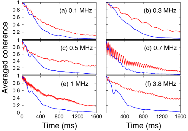
Figure 8.6: Simulations of coherence decays of a set of proximate nuclear qubits corresponding to a range of electron-qubit hyperfine couplings $J_{A}$ in MHz. The blue lines correspond to isotropic electron-bath coupling only and yield $T_{2}\approx 0.2-0.3$ s; red lines show the effect of symmetry reduction due to the anisotropy of couplings: we compare the effect of desymmetrisation if we constrain EPs to have in addition the same orientation condition (i.e. same $(\hat{\bf{n}}_{B}\cdot{\bf n})^{2}$). The effect is to produce $T_{2}$ in the seconds timescale. Figure adapted from Guichard et al. (2015).

8.5 Coherence Times

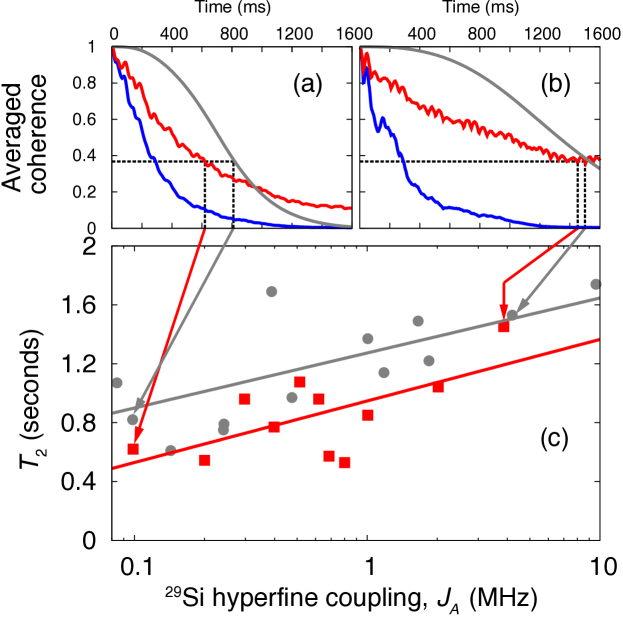
Figure 8.7: Top panels: Calculated Hahn echo decays for proximate spins in a Si:P system in natural silicon for (a) $J_{A}=0.1$ MHz and (b) $J_{A}=3.8$ MHz, where $J_{A}$ is the hyperfine coupling between the proximate spin and the donor electron. Red or blue correspond to decoherence driven by equivalent pairs (EP) while grey corresponds to far bath decoherence. The blue lines include only the isotropic part of the electron-bath hyperfine interaction, while the red lines include both isotropic and anisotropic contributions. Bottom panel (c): Calculated $T_{2}$ values from both models (red dots for EP model and grey dots for far bath). There is a weak trend for $T_{2}$ to increase as the hyperfine coupling increases (red line is a fit), possibly indicative of the decreasing density of EPs as the distance from the donor site $R\to 0$. In the far bath model, the slight increase in decoherence with lower $J_{A}$ (grey line) reflects the fact that the lower $J_{A}$ proximate spins are slightly closer to the far bath. Coherence times were obtained from decays averaged over 100 spatial realisations of the bath, but typical single realisations gave the same timescale of decoherence. Figure adapted from Guichard et al. (2015).

Coherence times from calculated coherence decays employing each model and for a representative set of proximate nuclear spins (quantified by $J_{A}$) are shown in Figure 8.7. Example coherence decays are also shown in Figure 8.7. In both cases, $T_{2}$ is of order 1 s with a weak dependence on $J_{A}$ – the coherence times tend to increase with larger $J_{A}$, a trend also seen in the experiments in Wolfowicz et al. (2015b).

For the EP model, we treat the anisotropic correction simply as a symmetry lowering effect (see top panel of Figure 8.7). This is plausible as the resultant detuning would be extremely large. Presently, it is not possible to fully include anisotropy using the Kohn-Luttinger wavefunction. The dipolar correction within this framework was included with a Heaviside function (Section 2.4.3), and is thus neglected for $R\lesssim 20$ Å. Given other uncertainties, the two EP calculations (with and without the anisotropy correction) in the top panels of Figure 8.7 provide an upper and a lower bound to $T_{2}$. As both results are on the seconds timescales, they suffice for the practical aim of establishing the proximate nuclear spins as useful qubits.

If the actual Si:P wavefunction exhibits a degree of spatial symmetry comparable with the Kohn-Luttinger wavefunction, then the EPs could be the dominant mechanism, albeit only slightly. However, it is likely that such symmetries are at least partly broken; in that case, the far bath would limit $T_{2}$. Given the uncertainties in the wavefunction model, at present it is not possible to determine accurately the contributions of EPs relative to the far bath, but fortuitously as the timescales are comparable, one can still conclude that the resulting $T_{2}$ is about 1 s.

To facilitate comparison with ensemble experiments, the EP results are averaged over many realisations (the far bath model coherence decays are almost completely insensitive to ensemble averaging). In the EP model, decoherence is primarily due to the indirect flip-flop process and this arises from only several dozen such EPs. Thus, although results from single donors fluctuate between realisations, the corresponding order of magnitude for $T_{2}$ remains on the 1 s timescale, whether ensemble averaging is carried out or not. The exception is the atypical realisation where the central spin happens to have an equivalent site it can directly flip-flop with. For proximate central spins, which occur usually in inner shells with $n_{s}=4,8,12$, this is unlikely. We find that the small subset of such realisations decohere rapidly. They contribute little to the ensemble averaged $T_{2}\sim 1$ s values but would clearly be unsuitable as qubit registers unless some strategy to exploit the degeneracy is envisaged. Finally and surprisingly, although the decay curves have a different shape, the $T_{2}$ values from both models are comparable.

8.6 Conclusion

Here we investigated the coherence of nuclear spins lying within the so-called “frozen core” surrounding the hybrid qubit in silicon, within a quantum bath framework. We also calculated the coherence using a very large far bath of spins lying outside the frozen core. We introduced a previously unstudied model, based on equivalent pairs (EPs) deep within the frozen core, which we argue would limit the coherence of proximate nuclear spins – provided the electronic wavefunction has the symmetries of the Kohn-Luttinger wavefunction (or even an alternative model with comparable levels of symmetry). Within the EP model, decoherence is primarily due to an indirect flip-flop process arising from a few dozen such EPs. Given the importance of carefully locating the few dozen or so most important EPs which can be quite widely separated, distance or coupling strength thresholds which are usually applied for spin bath decoherence are not reliable. The EP model of dephasing is quite generic: equivalent sites may play a role in any solid state qubit system with a sufficiently dense nuclear spin bath. Our quantitative results, however, are at best indicative. A more refined investigation could consider improved wavefunctions (Pica et al., 2014) and more detailed inclusion of the effect of anisotropy. Experimental investigations including dependence on symmetry-breaking mechanisms (such as crystal orientation and strain) will be useful to test our proposal of the EP model.

In summary, we considered two decoherence models for proximate nuclear qubits, either of which, given certain assumptions, might contribute. Both models predict ²⁹Si nuclear spin coherence times of order 1 s (using only a Hahn spin echo and no higher dynamical decoupling), which is consistent with recent experimental measurements (Wolfowicz et al., 2015b) showing such spins could be useful as potential qubits. If electronic symmetries are important, then a strategy for breaking such symmetries with external fields might be considered to obtain an even longer $T_{2}$; if the far bath is dominant, partial isotopic enrichment might be more useful (consideration of ²⁹Si nuclear spin registers in the present study naturally precludes full enrichment). We note that below 5 K, the electronic relaxation time $T_{1}$ is also above 1 s and would not limit the nuclear spin coherence.

9  |  Conclusions

The work presented in this thesis is the first theoretical study of decoherence of hybrid electron-nuclear spin qubits driven by a quantum spin bath, and also of nuclear qubits proximate to the hybrid qubit. By considering the full quantum state-mixing of the hybrid qubit in many-body calculations of coherence decays using the cluster correlation expansion (CCE), we obtain coherence times in perfect agreement with experiment across orders of magnitude variation with applied magnetic field and for an extensive set of resonant transitions. We also propose two decoherence mechanisms for proximate nuclear qubits: the equivalent pair and the far bath models, but expect the far bath to dominate experimental coherence decays because equivalent pair decoherence relies heavily on the symmetries of an approximate theoretical model for the donor wavefunction.

The physical system we use to implement the hybrid qubit is the mixed donor in silicon, focusing in particular on bismuth donors due to their atypically strong state-mixing. As for the quantum bath, we consider the natural spin-1/2 bath of silicon. However, we expect our theoretical methods to be applicable to other solid-state systems such as quantum dots or nitrogen vacancy centres in diamond. Our numerical CCE implementation is capable of handling any complex multi-spin central and bath Hamiltonians (see Appendix A for details of the code).

Of interest to the experimental quantum information processing community, we provide the theoretical means for reliable calculations of coherence times of hybrid qubits in all magnetic field regimes, including the case of the simple unmixed qubit. We also demonstrate how to enhance coherence times using operation at optimal working points (OWPs), by employing dynamical decoupling pulse sequences, or by combining the two methods. We derive a closed-form formula for coherence times which gives remarkably accurate predictions and is simple to use despite capturing the qubit-bath back-action without the need for a detailed numerical many-body calculation. The first pulsed magnetic resonance (ENDOR) experiments were presented for bismuth donors in the silicon spin bath, using which we find clear spectroscopic signatures of OWPs and characterise the hybrid qubit-nuclear spin bath interaction Hamiltonian. The pulsed experiments also demonstrate the feasibility of controlling proximate nuclear impurity spins.

When it comes to addressing more fundamental issues such as the extent to which classical magnetic field fluctuations are valid for describing decoherence driven by quantum baths or the role of many-body correlations in qubit-bath dynamics, we demonstrate that the hybrid qubit in a nuclear spin bath presents a good test bed for investigating such issues. In particular, we demonstrate that near OWP regions, a classical noise model based on frequency-field gradients does not reliably reproduce coherence times. The formula for coherence times also identifies clear differences between the classical and quantum bath models. In addition, we present the only case where the usual qubit-bath correlations from pairs of bath spins are almost entirely diminished and clusters of three spins in the many-body bath are required for converged coherence decays. This occurs near OWPs and for low to moderate orders of dynamical decoupling.

Throughout our presentation, we have compared most of our theoretical results with experimental measurements, finding excellent agreement in nearly all cases. In particular, theory-experiment comparisons were made for coherence calculations of the hybrid qubit for forbidden transitions, ESR-type and NMR-type transitions, near and far from OWPs and by combining OWPs with dynamical decoupling. Our predicted timescale of decoherence for proximate nuclear qubits also agrees with experiment.

A brief summary of the main outcomes of the work was also given in Section 1.2. For the rest of this chapter, we focus on the potential of the hybrid qubit (or a mixed electron-nuclear spin system) for quantum information applications, and discuss other future work motivated by our results, including a proposal for isolating increasing orders of many-body correlations.

It is clear that the hybrid qubit offers significant advantages for quantum computing and memory applications compared to the case of uncoupled electronic or nuclear spins. We focus on three aspects: fast quantum control at forbidden transitions, operation at OWPs, and coherence enhancement of proximate nuclear spins.

First, operating at ESR-forbidden transitions in the hybrid regime gives a factor of 125 speed-up of quantum control relative to the high-field regime albeit at the expense of shorter coherence times; if longer (pure nuclear) coherence times are required (i.e. for memory rather than processing), the magnetic field may be ramped up to the high-field regime. Nevertheless, qubit manipulation times are five orders of magnitude shorter than coherence times in the hybrid regime. We established that in this forbidden transition regime of proven fast control, coherence times are limited by nuclear spin diffusion. Unfortunately, this 4 GHz excitation frequency region does not correspond to an OWP region. Thus, coherence times here could be extended by isotopic enrichment or dynamical decoupling. Second, for transitions with OWPs, two orders of magnitude enhancement in coherence times are achievable without the need for any isotopic enrichment or multi-pulse dynamical decoupling control. Fast microwave-pulsed quantum control is also achievable for ESR-type OWPs. Further enhancement of coherence at OWPs in natural silicon is possible, but requires a large number of dynamical decoupling pulses – of order hundreds for a single order of magnitude enhancement. Third, the hybrid qubit (in the unmixed regime) features a frozen core, protecting proximate nuclear spins from quantum bath noise and leading to almost three orders of magnitude nuclear coherence time enhancement, thus making proximate nuclei ideal for use as quantum registers, while the hybrid qubit is employed for processing. Finally, we note that a universal set of quantum gates using the hybrid qubit are detailed in Mohammady et al. (2012).

9.1 Future Work

As mentioned above, methods similar to those presented herein may be applicable to other spin systems. For OWPs in donors, a host nuclear spin quantum number exceeding $I=1/2$ is required. Hence, all silicon donors except for phosphorus can implement the hybrid qubit. To date, all single-donor measurements have been made on phosphorus donors and all OWP experiments on ensembles of bismuth donors. Systems of interest in quantum information processing which warrant modification or extension of our methods include quantum dots (Webster et al., 2014), especially coupled dots (Weiss et al., 2012, 2013) and also nitrogen vacancy centres in diamond (Zhao et al., 2012a). Also, some materials have a rich variety of nuclear impurities; hence, heteronuclear spin baths become relevant.

Better knowledge of the donor electron wavefunction is expected to improve our results for both the hybrid qubit and proximate qubits. More accurate models than the standard Kohn-Luttinger model exist, such as the model presented in Pica et al. (2014). First, it is expected that limitations of the Kohn-Luttinger wavefunction contribute to the small deviations between calculated and measured coherence decays, whether for proximate nuclear or hybrid qubit decoherence. More importantly, the equivalent pair model relies heavily on symmetries of the wavefunction. One way of gaining more information about the wavefunction is to better characterise the nuclear spin bath by performing continuous wave magnetic resonance which offers higher resolution than pulsed methods and which can be used to assign hyperfine couplings of the donor electron spin to nuclear spin impurity positions or shells (Hale and Mieher, 1969a, b). We note that if the equivalent pair model is confirmed by some other means, it could be used to test the validity of symmetries in wavefunction models. Also, in characterising the interaction to the spin bath, a future improvement is thorough assessment of the errors in obtaining the anisotropic hyperfine couplings from rotation spectra, for which data with higher angular resolution and knowledge of all relevant crystal directions are needed. Finally, understanding the dependence of sidebands in ENDOR spectra on the radio frequency pulse length should lead to an improved comparison between calculated and measured peak positions at low field.

The validity of the analytical formula for coherence times near OWPs remains partially understood. The field-independent prefactor in the formula was derived from pair correlations. The short time approximation was also used. However, it is not entirely clear how the formula is successful for longer times. In fact, the convolution of decays predicted by the formula near OWPs does show significant discrepancy with experiment at longer times (beyond $T_{2}$) as seen in Figure 5.11. Three-clusters are essential for coherence decays as a function of time reaching zero-coherence near OWPs. More remarkable is that the formula gives accurate predictions for a range of OWPs (where the pair of polarisations vary by about an order of magnitude) and with large variations in coherence time regardless of the fact that the derivation is based on an analysis of only pair correlations. One thing that is clear is that the field-dependent component of the formula is a robust feature in all regimes. Also, more work is needed to understand the factor of about 2 to 3 difference between the Hahn spin echo and FID coherence times near OWPs, and the reduction of this factor to about 1.1 as the field is set far from the OWP.

As for comparing classical and quantum bath decoherence, very recently it was reported that the nuclear spin bath is of “semi-classical” nature near OWPs (Ma et al., 2015). This seems to contradict a main result in this thesis. However, a closer look at the study reveals that a quantum many-body calculation (CCE) is in fact carried out to determine the correlation function of the bath which includes a back-action term ($|P_{u}|+|P_{l}|$). Nevertheless, at the start of the thesis, we state that qubit-bath back-action (or central state dependence of the bath evolution) is a defining characteristic of what we mean by a quantum bath, and we compare to previous classical models involving only a property of the qubit (frequency-field gradient). Hence, the conflict between our work and the study in Ma et al. (2015) is simply resolved by the fact that we use a different definition of classicality than the one in Ma et al. (2015).

For isotopically enriched samples, where the nuclear spin bath is effectively eliminated, decoherence is driven by donor-donor processes. The same spin system, a donor spin, constitutes both the central system and bath. Decoherence is driven by either spin diffusion from a flip-flopping bath of donors coupled to the central donor (indirect flip-flops) or flip-flops between the central donor and a bath donor (a relaxation-type process involving single-spin bath clusters and known as direct flip-flops). Indirect flip-flops are similar to the nuclear spin diffusion process and are expected to be suppressed near OWPs. However, it is not clear if there are any practically accessible sweet-spots for suppressing direct flip-flops (see for example, Monteiro (2014)), which limit coherence times in enriched silicon at OWPs. If refocusing pulses are applied on the all-dipolar donor system, decoherence is introduced as a process known as instantaneous diffusion (Tyryshkin et al., 2012) which reduces coherence times from seconds to the millisecond timescale. Again, it is not entirely understood whether or not special magnetic field regions are experimentally feasible for the hybrid qubit for suppressing this process (Monteiro, 2014). In order to obtain accurate coherence decays for donor-donor decoherence, a modified CCE with external cluster awareness is needed for good accuracy (Witzel et al., 2012). Note that near OWPs, coherence times from donor-donor processes can be comparable to nuclear bath coherence times in natural silicon, provided the donor concentration is high enough. Also, dynamical decoupling for donor-donor processes should be investigated, as well as in combination with OWPs. Finally, it has been previously demonstrated for phosphorus-doped silicon that line-broadening effects caused by nuclear impurity spins in the bath suppress donor-donor flip-flops (Witzel et al., 2010), thus future studies must consider partial isotopic enrichment and a mixture of donor-donor and impurity-related decoherence mechanisms; i.e., what is the ideal donor and impurity concentration for maximizing coherence times?

The width of spectral lines in a spin impurity environment presents a limit to how closely the magnetic field can be adjusted towards the OWP. By investigating partial enrichment, the best compromise between coherence times of the hybrid qubit and the density of proximate nuclear spins could be established. As for proximate nuclear qubits, we note that there is no $T_{2}$ measurement of a single proximate spin. Coherence decays from single realisations may show oscillations due to the few equivalent pairs. Also, studies on wavefunction symmetry-breaking mechanisms could provide a good test of our equivalent pairs model.

It should be mentioned that as an OWP is approached, the likelihood of numerical divergences for high-order CCE increases. This is especially true for four-clusters and surprisingly less so for five-clusters. The reason is not fully understood but the divergences depend on the choice of bath realisations, are mitigated by averaging over many realisations and most likely result numerically from divisions by near-zeros.

Finally, additional work is needed to establish the many-body nature of the silicon spin bath at OWPs. The 3-body correlations can have their origin in three-clusters containing three flip-flopping spins or renormalised flip-flopping pairs; i.e. two-clusters with detuning from frozen external spins. The possibility of isolating many-body correlations of increasing order (i.e. 3-body, 4-body, …) as the field approaches closer to an OWP should also be investigated. Since the linewidth in natural silicon limits how close to an OWP the magnetic field can be set, many-body correlations should be studied for increasingly sparse spin baths with reduced impurity concentrations.

Appendix A SpinDec Library

A.1 Overview

SpinDec is a C++ library for spin decoherence calculations written by S.J.B.. It is free to use and can be downloaded from Bitbucket or CCPForge:

https://bitbucket.org/sbalian/spindec

https://ccpforge.cse.rl.ac.uk/gf/project/spindec/

It should be cited as it appears in the thesis bibliography (see reference Balian (2015) and Section A.5 for its BibTeX entry).

The code solves for the many-body dynamics of a central spin system coupled to an interacting spin bath. It supports any complex multi-spin Hamiltonian for both the central and bath Hamiltonians. Spin Hamiltonians can be constructed by creating abstract spin interaction graphs and defining edges for interactions among single spin vertices.

The cluster correlation expansion is implemented, special methods for donors in silicon are available and methods are included for CPMG control. The repository also includes an executable for calculating CPMG dephasing of donors in silicon interacting with a ²⁹Si nuclear spin bath. Special methods for quantum dots and heteronuclear spin baths are under development.

This appendix includes installation and usage instructions for SpinDec.

A.2 Installation

The code has been tested on Linux and Mac OS X. Installation requirements are as follows:

• Eigen (free): For linear algebra.

  http://eigen.tuxfamily.org

• CMake (free): For building and installing.

  http://www.cmake.org/

• boost (free): For program options. Only required for executable.

  http://www.boost.org/

• Optional: Intel MKL optimization for Eigen.

  https://software.intel.com/en-us/intel-mkl/

The following installation instructions are for a Unix-like environment without root privileges. It also assumes you have Mercurial (hg) installed.

To get the code, type in a terminal with bash,

⬇

mkdir spindec

cd spindec

hg clone http://www.bitbucket.org/sbalian/spindec .

Now let’s build it.

⬇

mkdir build

cd build

cmake .. -DCMAKE_INSTALL_PREFIX=/home/myusrname

make -j4 all

make install

The argument to cmake defines the installation location (here set to ‘myusrname’, which you should change to your user name). If you invoke cmake without specifying the location, it will install to your default system prefix (requires root). The -j4 option to make parallelises the build process using 4 cores. Make sure this number does not exceed the number of cores for your machine.

If all went well, you should now have the static library and executables. The library, headers and executables should be located in the following directories respectively: /home/myusrname/lib, /home/myusrname/include, /home/myusrname/bin.

Optionally, to enable MKL optimization in Eigen, pass -DSPINDEC_USE_MKL=ON to cmake. Obviously, you will need the proprietary MKL libraries for this step. For further customization, see the included file CMakeLists.txt (you will need to understand cmake).

A.3 Usage

Documentation generated with doxygen is available, detailing the structure of the code and explaining its use. To use SpinDec, just include the SpinDec/base.h header in your source and link with libspindec. Also, the executable for nuclear spin diffusion spindec-dsnsd has a ---help option.

Help can also be found directly in header files (.h extension in include/SpinDec). Source files (.cpp extension in src/) may contain more information, usually geared more towards implementation. See Section A.4 for examples of usage.

A.4 Examples

First, follow the instructions under “Installation” (Section A.2). Then, open the file spindec/tests/spindec-test-cce.cpp to see the source with comments on the example problem. Using the cluster correlation expansion up to 3rd order, it calculates the Hahn spin echo decay of a central donor spin in silicon for a nuclear spin bath (spin-1/2 ²⁹Si with a natural abundance of 4.7%). To see the decay, run spindec-test-cce. The test executable is not installed, so run it in the build directory. The source for spindec-dsnsd (src/spindec-dsnsd.cpp) should also serve as a good example.

A.5 License and How to Cite

SpinDec is free to use under the GNU General Public License. See LICENSE file for more details. If you use any part of the code in a publication, please cite it as follows:

S. J. Balian, Spindec: C++ Library for Spin Decoherence, http://www.bitbucket.org/sbalian/spindec (2011-2015).

Below is the BibTeX entry:

⬇

@misc{SpinDec,

title = {SpinDec: C++ Library for Spin Decoherence},

author = {Balian, Setrak J.},

howpublished = {http://www.bitbucket.org/sbalian/spindec},

year = {2011--2015}

}

A.6 Version and History

As of June 15, 2015 the version number is 0.9 (late-stage beta - debugged, tested, profiled, optimized and checked for memory leaks). SpinDec is based on bits and pieces of code for certain spin baths and central spin systems. These were written by S.J.B. starting in 2011. Methods used to efficiently fill Hamiltonian matrix elements were originally written in Fortran by Professor Tania Monteiro. Development for SpinDec as an open-source project started in May 2013.

Appendix B Pauli Operators

Any two-level observable can be described by linear combinations of the Pauli operators $\hat{\sigma}_{k}$, $k=1,2,3$ (Audretsch, 2007) and the $2\times 2$ identity. The operators act on the 2-dimensional Hilbert space and satisfy

$$\hat{\sigma}^{i}\hat{\sigma}^{j}=\delta_{ij}\hat{\mathds{1}}+i\sum_{k=1}^{3}\epsilon_{ijk}\hat{\sigma}^{k},$$ (B.1)

where $i,j=1,2,3$, $\delta_{ij}$ is the Kronecker delta ($\delta_{ij}=1$ for $i=j$, $\delta_{ij}=0$ for $i\neq j$), $\hat{\mathds{1}}$ is the identity operator and the tensor $\epsilon_{ijk}$ is totally antisymmetric in all indices with $\epsilon_{123}=1$. Equivalently, the condition in Equation (B.1) can be written in terms of the commutators and anti-commutators

$$\left[\hat{\sigma}^{i},\hat{\sigma}^{j}\right]=2i\sum_{k=1}^{3}\epsilon_{ijk}\hat{\sigma}^{k},$$ (B.2)

$$\left\{\hat{\sigma}^{i},\hat{\sigma}^{j}\right\}=2\delta_{ij}\hat{\mathds{1}}.$$ (B.3)

The Pauli vector in the Cartesian basis $\hat{\bm{\sigma}}=(\hat{\sigma}_{x},\hat{\sigma}_{y},\hat{\sigma}_{z})$ is often used to refer to the operators. The operators are Hermitian ($(\hat{\sigma}^{k})^{\dagger}=\hat{\sigma}^{k}$), unitary ($(\hat{\sigma}^{k})^{\dagger}=(\hat{\sigma}^{k})^{-1}$) and traceless ($\text{Tr}[\hat{\sigma}^{k}]=0$), and have eigenvalues $+1$ and $-1$. Taking the orthonormal basis of eigenvectors of $\hat{\sigma}_{z}$ as $\{\left|{0}\right\rangle,\left|{1}\right\rangle\}$, the matrix representations of the operators in this basis are the Pauli matrices:

$$\bm{\sigma}^{x}=\left(\begin{array}[]{cc}0&1\\ 1&0\end{array}\right), \bm{\sigma}^{y}=\left(\begin{array}[]{cc}0&-i\\ i&0\end{array}\right), \bm{\sigma}^{z}=\left(\begin{array}[]{cc}1&0\\ 0&-1\end{array}\right).$$ (B.10)

The electron has a total spin quantum number $S=1/2$ and its spin angular momentum operators are related to the Pauli operators according to $\hat{\bf S}=(\hat{S}^{x},\hat{S}^{y},\hat{S}^{z})=\hat{\bm{\sigma}}/2$. For a nuclear spin-1/2, we write $I=1/2$ and $\hat{\bf I}=\hat{\bm{\sigma}}/2$.

In quantum computing, the Pauli operators represent simple single-qubit gates. For example, the Pauli-$X$ gate ($\left|{0}\right\rangle\left\langle{1}\right|+\left|{1}\right\rangle\left|{0}\right\rangle$) flips $\left|{0}\right\rangle$ ($\left|{1}\right\rangle$) to $\left|{1}\right\rangle$ ($\left|{0}\right\rangle$) (Nielsen and Chuang, 2010).

Appendix C Silicon Crystal Structure

Silicon forms the diamond cubic crystal structure (Kittel, 1996). The diamond cubic is two face-centred cubic (FCC) lattices, one displaced from the other by a distance of $\frac{1}{4}a_{0}$ along the body diagonals, where $a_{0}$ is the conventional cubic cell lattice parameter (i.e. side length of the cubic cell). For silicon, $a_{0}=5.43$ Å. The conventional cubic cell of the diamond cubic is illustrated in Figure C.1.

Figure C.1: Conventional cubic cell of the diamond cubic crystal structure. The nearest neighbors distances (illustrated relative to the black atom) are $\tfrac{\sqrt{3}}{4}a_{0}$ (red), $\tfrac{\sqrt{2}}{2}a_{0}$ (blue), $\tfrac{\sqrt{11}}{4}a_{0}$ (green) and $a_{0}$ (purple), where $a_{0}$ is the lattice parameter. In Miller index notation (Kittel, 1996), [100], [010] and [001] correspond to the directions along $\hat{\bf x}$, $\hat{\bf y}$ and $\hat{\bf z}$ respectively. For example, [111] is along the body diagonal. Figure adapted from Balian et al. (2014).

The crystal structure can also be described by a simple cubic lattice and an 8-site basis. We represent all atomic sites (the crystal structure) by an integer vector ${\bf n}=(n_{1},n_{2},n_{3})$, the integers obtained from modulo 4 translations in all directions of the 8 basis vectors. The 8 basis vectors are: (0,0,0), (0,2,2), (2,0,2), (2,2,0), (1,1,3), (1,3,1), (3,1,1), and (3,3,3). The transformation to convert from integer to real space ${\bf R}$ is

$${\bf R}_{(n_{1},n_{2},n_{3})}=\frac{a_{0}}{4}\left(n_{1}\hat{\bf x}+n_{2}\hat{\bf y}+n_{3}\hat{\bf z}\right),$$ (C.1)

in Cartesian coordinates, where the axes are parallel to those of the conventional cubic cell.

References

- Abe et al. (2004) Abe, E., K. M. Itoh, J. Isoya, and S. Yamasaki (2004), Phys. Rev. B 70, 033204.
- Abe et al. (2010) Abe, E., A. M. Tyryshkin, S. Tojo, J. J. L. Morton, W. M. Witzel, A. Fujimoto, J. W. Ager, E. E. Haller, J. Isoya, S. A. Lyon, M. L. W. Thewalt, and K. M. Itoh (2010), Phys. Rev. B 82, 121201.
- Akhtar et al. (2012) Akhtar, W., V. Filidou, T. Sekiguchi, E. Kawakami, T. Itahashi, L. Vlasenko, J. J. L. Morton, and K. M. Itoh (2012), Phys. Rev. Lett. 108, 097601.
- Audretsch (2007) Audretsch, J. (2007), Entangled Systems, New Directions in Quantum Physics (Wiley-VCH, Weinheim, Germany).
- Balian (2015) Balian, S. J. (2011–2015), “SpinDec: C++ Library for Spin Decoherence,” http://www.bitbucket.org/sbalian/spindec.
- Balian et al. (2012) Balian, S. J., M. B. A. Kunze, M. H. Mohammady, G. W. Morley, W. M. Witzel, C. W. M. Kay, and T. S. Monteiro (2012), Phys. Rev. B 86, 104428.
- Balian et al. (2015) Balian, S. J., R.-B. Liu, and T. S. Monteiro (2015), Phys. Rev. B 91, 245416.
- Balian et al. (2014) Balian, S. J., G. Wolfowicz, J. J. L. Morton, and T. S. Monteiro (2014), Phys. Rev. B 89, 045403.
- Bar-Gill et al. (2012) Bar-Gill, N., L. Pham, C. Belthangady, D. Le Sage, P. Cappellaro, J. Maze, M. Lukin, A. Yacoby, and R. Walsworth (2012), Nat. Commun. 3, 858.
- Bar-Gill et al. (2013) Bar-Gill, N., L. M. Pham, A. Jarmola, D. Budker, and R. L. Walsworth (2013), Nat. Commun. 4, 1743.
- Belli et al. (2011) Belli, M., M. Fanciulli, and N. V. Abrosimov (2011), Phys. Rev. B 83, 235204.
- Bernien et al. (2013) Bernien, H., B. Hensen, W. Pfaff, G. Koolstra, M. Blok, L. Robledo, T. Taminiau, M. Markham, D. Twitchen, L. Childress, and R. Hanson (2013), Nature (London) 497, 86.
- Biercuk et al. (2009) Biercuk, M. J., H. Uys, A. P. VanDevender, N. Shiga, W. M. Itano, and J. J. Bollinger (2009), Nature (London) 458, 996.
- Breuer and Petruccione (2002) Breuer, H., and F. Petruccione (2002), The Theory of Open Quantum Systems (Oxford University Press, Oxford).
- Cappellaro et al. (2009) Cappellaro, P., L. Jiang, J. S. Hodges, and M. D. Lukin (2009), Phys. Rev. Lett. 102, 210502.
- Carr and Purcell (1954) Carr, H. Y., and E. M. Purcell (1954), Phys. Rev. 94, 630.
- Chekhovich et al. (2015) Chekhovich, E., M. Hopkinson, M. Skolnick, and A. Tartakovskii (2015), Nat. Commun. 6, 6348.
- Cohen-Tannoudji et al. (1977) Cohen-Tannoudji, C., B. Diu, and F. Laloe (1977), Quantum Mechanics Volume 2 (Wiley-VCH).
- Dementyev et al. (2003) Dementyev, A. E., D. Li, K. MacLean, and S. E. Barrett (2003), Phys. Rev. B 68, 153302.
- Dreher et al. (2012) Dreher, L., F. Hoehne, M. Stutzmann, and M. S. Brandt (2012), Phys. Rev. Lett. 108, 027602.
- Du et al. (2009) Du, J., X. Rong, N. Zhao, Y. Wang, J. Yang, and R. B. Liu (2009), Nature (London) 461, 1265.
- Falci et al. (2005) Falci, G., A. D’Arrigo, A. Mastellone, and E. Paladino (2005), Phys. Rev. Lett. 94, 167002.
- Feher (1959) Feher, G. (1959), Phys. Rev. 114, 1219.
- Fraval et al. (2005) Fraval, E., M. J. Sellars, and J. J. Longdell (2005), Phys. Rev. Lett. 95, 030506.
- Fu et al. (2004) Fu, K.-M. C., T. D. Ladd, C. Santori, and Y. Yamamoto (2004), Phys. Rev. B 69, 125306.
- Fuechsle et al. (2012) Fuechsle, M., J. A. Miwa, S. Mahapatra, H. Ryu, S. Lee, O. Warschkow, L. C. L. Hollenberg, G. Klimeck, and M. Y. Simmons (2012), Nature Nanotech. 7 (4), 242.
- Gaebel et al. (2006) Gaebel, T., M. Domhan, I. Popa, C. Wittmann, P. Neumann, F. Jelezko, J. R. Rabeau, N. Stavrias, A. D. Greentree, S. Prawer, J. Meijer, J. Twamley, P. R. Hemmer, and J. Wrachtrup (2006), Nat. Phys. 2, 408.
- George et al. (2013) George, R. E., J. P. Edwards, and A. Ardavan (2013), Phys. Rev. Lett. 110, 027601.
- George et al. (2010) George, R. E., W. Witzel, H. Riemann, N. V. Abrosimov, N. Nötzel, M. L. W. Thewalt, and J. J. L. Morton (2010), Phys. Rev. Lett. 105, 067601.
- Greenland et al. (2010) Greenland, P. T., S. A. Lynch, A. F. G. van der Meer, B. N. Murdin, C. R. Pidgeon, B. Redlich, N. Q. Vinh, and G. Aeppli (2010), Nature (London) 465 (7301), 1057.
- Guichard et al. (2015) Guichard, R., S. J. Balian, G. Wolfowicz, P. A. Mortemousque, and T. S. Monteiro (2015), Phys. Rev. B 91, 214303.
- Hahn (1950) Hahn, E. L. (1950), Phys. Rev. 80, 580.
- Hale and Mieher (1969a) Hale, E. B., and R. L. Mieher (1969a), Phys. Rev. 184, 739.
- Hale and Mieher (1969b) Hale, E. B., and R. L. Mieher (1969b), Phys. Rev. 184, 751.
- Hayashi et al. (2008) Hayashi, H., K. M. Itoh, and L. S. Vlasenko (2008), Phys. Rev. B 78, 153201.
- Ithier et al. (2005) Ithier, G., E. Collin, P. Joyez, P. J. Meeson, D. Vion, D. Esteve, F. Chiarello, A. Shnirman, Y. Makhlin, J. Schriefl, and G. Schön (2005), Phys. Rev. B 72, 134519.
- Kane (1998) Kane, B. E. (1998), Nature (London) 393, 133.
- Kawakami et al. (2014) Kawakami, E., P. Scarlino, D. Ward, F. Braakman, D. Savage, M. Lagally, M. Friesen, S. Coppersmith, M. Eriksson, and L. Vandersypen (2014), Nature Nanotech. 9, 666.
- Khutsishvili (1967) Khutsishvili, G. R. (1967), Sov. Phys. – JETP 25, 1050.
- Kittel (1996) Kittel, C. (1996), Introduction to Solid State Physics, Seventh Edition (Wiley, New Jersey).
- Klauder and Anderson (1962) Klauder, J. R., and P. W. Anderson (1962), Phys. Rev. 125, 912.
- Koehl et al. (2011) Koehl, W. F., B. B. Buckley, F. J. Heremans, G. Calusine, and D. D. Awschalom (2011), Nature (London) 479 (7371), 84.
- Kolkowitz et al. (2012) Kolkowitz, S., Q. P. Unterreithmeier, S. D. Bennett, and M. D. Lukin (2012), Phys. Rev. Lett. 109, 137601.
- Koppens et al. (2008) Koppens, F. H. L., K. C. Nowack, and L. M. K. Vandersypen (2008), Phys. Rev. Lett. 100, 236802.
- Ladd et al. (2002) Ladd, T. D., J. R. Goldman, F. Yamaguchi, Y. Yamamoto, E. Abe, and K. M. Itoh (2002), Phys. Rev. Lett. 89, 017901.
- Ladd et al. (2005) Ladd, T. D., D. Maryenko, Y. Yamamoto, E. Abe, and K. M. Itoh (2005), Phys. Rev. B 71, 014401.
- Lang et al. (2015) Lang, J. E., R.-B. Liu, and T. S. Monteiro (2015), ArXiv:1502.07960.
- de Lange et al. (2012) de Lange, G., T. van der Sar, M. Blok, Z.-H. Wang, V. Dobrovitski, and R. Hanson (2012), Sci. Rep. 2.
- de Lange et al. (2010) de Lange, G., Z. H. Wang, D. Riste, V. V. Dobrovitski, and R. Hanson (2010), Science 330, 60.
- Latta et al. (2011) Latta, C., A. Srivastava, and A. Imamoğlu (2011), Phys. Rev. Lett. 107, 167401.
- Lee et al. (2008) Lee, B., W. M. Witzel, and S. Das Sarma (2008), Phys. Rev. Lett. 100, 160505.
- Liu et al. (2007) Liu, R.-B., W. Yao, and L. J. Sham (2007), New Journal of Physics 9 (7), 226.
- Ma et al. (2015) Ma, W.-L., G. Wolfowicz, S.-S. Li, J. J. L. Morton, and R.-B. Liu (2015), ArXiv:1505.01604.
- Ma et al. (2014) Ma, W.-L., G. Wolfowicz, N. Zhan, S.-S. Li, J. J. L. Morton, and R.-B. Liu (2014), Nat. Commun. 5, 4822.
- Makhlin et al. (2004) Makhlin, Y., G. Schon, and A. Shnirman (2004), Chemical Physics 296 (2–3), 315.
- Makhlin and Shnirman (2004) Makhlin, Y., and A. Shnirman (2004), Phys. Rev. Lett. 92, 178301.
- Maniscalco and Petruccione (2006) Maniscalco, S., and F. Petruccione (2006), Phys. Rev. A 73, 012111.
- Martinis et al. (2003) Martinis, J. M., S. Nam, J. Aumentado, K. M. Lang, and C. Urbina (2003), Phys. Rev. B 67, 094510.
- Maze et al. (2008) Maze, J. R., J. M. Taylor, and M. D. Lukin (2008), Phys. Rev. B 78, 094303.
- Mazzola et al. (2012) Mazzola, L., C. A. Rodríguez-Rosario, K. Modi, and M. Paternostro (2012), Phys. Rev. A 86, 010102.
- McCamey et al. (2010) McCamey, D., J. Van Tol, G. Morley, and C. Boehme (2010), Science 330, 1652.
- Meiboom and Gill (1958) Meiboom, S., and D. Gill (1958), Review of Scientific Instruments 29, 688.
- Mildren and Rabeau (2013) Mildren, R., and J. Rabeau (2013), Optical Engineering of Diamond, First Edition (Wiley-VCH) ch. 9, p. 292.
- Mohammady et al. (2010) Mohammady, M. H., G. W. Morley, and T. S. Monteiro (2010), Phys. Rev. Lett. 105, 067602.
- Mohammady et al. (2012) Mohammady, M. H., G. W. Morley, A. Nazir, and T. S. Monteiro (2012), Phys. Rev. B 85, 094404.
- Monteiro (2014) Monteiro, T. S. (2014), ArXiv:1412.2645.
- Morello et al. (2010) Morello, A., J. J. Pla, F. A. Zwanenburg, K. W. Chan, K. Y. Tan, H. Huebl, M. Mottonen, C. D. Nugroho, C. Yang, J. A. van Donkelaar, A. D. C. Alves, D. N. Jamieson, C. C. Escott, L. C. L. Hollenberg, R. G. Clark, and A. S. Dzurak (2010), Nature (London) 467, 687.
- Morley (2015) Morley, G. W. (2015), in Electron Paramagnetic Resonance, Vol. 24 (The Royal Society of Chemistry) pp. 62–76.
- Morley et al. (2013) Morley, G. W., P. Lueders, M. Hamed Mohammady, S. J. Balian, G. Aeppli, C. W. M. Kay, W. M. Witzel, G. Jeschke, and T. S. Monteiro (2013), Nature Mater. 12, 103.
- Morley et al. (2008) Morley, G. W., D. R. McCamey, H. A. Seipel, L.-C. Brunel, J. van Tol, and C. Boehme (2008), Phys. Rev. Lett. 101, 207602.
- Morley et al. (2010) Morley, G. W., M. Warner, A. M. Stoneham, P. T. Greenland, J. van Tol, C. W. M. Kay, and G. Aeppli (2010), Nature Mater. 9 (9), 725.
- Morton et al. (2006) Morton, J. J., A. M. Tyryshkin, A. Ardavan, S. C. Benjamin, K. Porfyrakis, S. Lyon, and G. A. D. Briggs (2006), Nature Physics 2, 40.
- Morton et al. (2005) Morton, J. J. L., A. M. Tyryshkin, A. Ardavan, K. Porfyrakis, S. A. Lyon, and G. A. D. Briggs (2005), Phys. Rev. Lett. 95, 200501.
- Morton et al. (2008) Morton, J. J. L., A. M. Tyryshkin, R. M. Brown, S. Shankar, B. W. Lovett, A. Ardavan, T. Schenkel, E. E. Haller, J. W. Ager, and S. A. Lyon (2008), Nature (London) 455, 1085.
- Muhonen et al. (2014) Muhonen, J. T., J. P. Dehollain, A. Laucht, F. E. Hudson, R. Kalra, T. Sekiguchi, K. M. Itoh, D. N. Jamieson, J. C. McCallum, A. S. Dzurak, and A. Morello (2014), Nature Nanotech. 9, 986.
- Müller et al. (2014) Müller, C., X. Kong, J.-M. Cai, K. Melentijević, A. Stacey, M. Markham, D. Twitchen, J. Isoya, S. Pezzagna, J. Meijer, J. F. Du, M. B. Plenio, B. Naydenov, L. P. McGuinness, and F. Jelezko (2014), Nat. Commun. 5, 4703.
- Cywiński (2014) Cywiński, L. (2014), Phys. Rev. A 90, 042307.
- Ng et al. (2011) Ng, H. K., D. A. Lidar, and J. Preskill (2011), Phys. Rev. A 84, 012305.
- Nielsen and Chuang (2010) Nielsen, M., and I. Chuang (2010), Quantum Computation and Quantum Information (Cambridge University Press, Cambridge).
- Peng et al. (2011) Peng, X., D. Suter, and D. A. Lidar (2011), Journal of Physics B: Atomic, Molecular and Optical Physics 44, 154003.
- Petersen et al. (2013) Petersen, E. S., A. M. Tyryshkin, S. A. Lyon, J. J. L. Morton, K. M. Itoh, and M. L. W. Thewalt (2013), in APS Meeting Abstracts, p. 26004.
- Pham et al. (2012) Pham, L. M., N. Bar-Gill, C. Belthangady, D. Le Sage, P. Cappellaro, M. D. Lukin, A. Yacoby, and R. L. Walsworth (2012), Phys. Rev. B 86, 045214.
- Pica et al. (2014) Pica, G., B. W. Lovett, R. N. Bhatt, and S. A. Lyon (2014), Phys. Rev. B 89, 235306.
- Pla et al. (2014) Pla, J. J., F. A. Mohiyaddin, K. Y. Tan, J. P. Dehollain, R. Rahman, G. Klimeck, D. N. Jamieson, A. S. Dzurak, and A. Morello (2014), Phys. Rev. Lett. 113, 246801.
- Pla et al. (2013) Pla, J. J., K. Y. Tan, J. P. Dehollain, W. H. Lim, J. J. Morton, F. A. Zwanenburg, D. N. Jamieson, A. S. Dzurak, and A. Morello (2013), Nature (London) 496, 334.
- Pla et al. (2012) Pla, J. J., K. Y. Tan, J. P. Dehollain, W. H. Lim, J. J. L. Morton, D. N. Jamieson, A. S. Dzurak, and A. Morello (2012), Nature (London) 489, 541.
- Reinhard et al. (2012) Reinhard, F., F. Shi, N. Zhao, F. Rempp, B. Naydenov, J. Meijer, L. T. Hall, L. Hollenberg, J. Du, R.-B. Liu, and J. Wrachtrup (2012), Phys. Rev. Lett. 108, 200402.
- Robledo et al. (2011) Robledo, L., L. Childress, H. Bernien, B. Hensen, P. F. Alkemade, and R. Hanson (2011), Nature (London) 477, 574.
- Saeedi et al. (2013) Saeedi, K., S. Simmons, J. Z. Salvail, P. Dluhy, H. Riemann, N. V. Abrosimov, P. Becker, H.-J. Pohl, J. J. L. Morton, and M. L. W. Thewalt (2013), Science 342, 830.
- Saikin et al. (2007) Saikin, S. K., W. Yao, and L. J. Sham (2007), Phys. Rev. B 75, 125314.
- Schliemann et al. (2002) Schliemann, J., A. V. Khaetskii, and D. Loss (2002), Phys. Rev. B 66, 245303.
- Schofield et al. (2003) Schofield, S. R., N. J. Curson, M. Y. Simmons, F. J. Rueß, T. Hallam, L. Oberbeck, and R. G. Clark (2003), Phys. Rev. Lett. 91, 136104.
- Schweiger and Jeschke (2001) Schweiger, A., and G. Jeschke (2001), Principles of pulse electron paramagnetic resonance spectroscopy (Oxford University Press, Oxford).
- Sekiguchi et al. (2010) Sekiguchi, T., M. Steger, K. Saeedi, M. L. W. Thewalt, H. Riemann, N. V. Abrosimov, and N. Nötzel (2010), Phys. Rev. Lett. 104, 137402.
- Shor (1996) Shor, P. W. (1996), in Foundations of Computer Science, 1996. Proceedings., 37th Annual Symposium on (IEEE) pp. 56–65.
- Simmons et al. (2011) Simmons, S., R. M. Brown, H. Riemann, N. V. Abrosimov, P. Becker, H.-J. Pohl, M. L. W. Thewalt, K. M. Itoh, and J. J. L. Morton (2011), Nature (London) 470, 69.
- Simon et al. (2010) Simon, C., M. Afzelius, J. Appel, A. Boyer de la Giroday, S. J. Dewhurst, N. Gisin, C. Y. Hu, F. Jelezko, S. Kroll, J. H. Muller, J. Nunn, E. S. Polzik, J. G. Rarity, H. De Riedmatten, W. Rosenfeld, A. J. Shields, N. Skold, R. M. Stevenson, R. Thew, I. A. Walmsley, M. C. Weber, H. Weinfurter, J. Wrachtrup, and R. J. Young (2010), The European Physical Journal D 58, 1.
- de Sousa and Das Sarma (2003a) de Sousa, R., and S. Das Sarma (2003a), Phys. Rev. B 67, 033301.
- de Sousa and Das Sarma (2003b) de Sousa, R., and S. Das Sarma (2003b), Phys. Rev. B 68, 115322.
- Steger et al. (2012) Steger, M., K. Saeedi, M. L. W. Thewalt, J. J. L. Morton, H. Riemann, N. V. Abrosimov, P. Becker, and H.-J. Pohl (2012), Science 336, 1280.
- Steger et al. (2011) Steger, M., T. Sekiguchi, A. Yang, K. Saeedi, M. E. Hayden, M. L. W. Thewalt, K. M. Itoh, H. Riemann, N. V. Abrosimov, P. Becker, and H.-J. Pohl (2011), J. Appl. Phys. 109, 102411.
- Stone (2005) Stone, N. J. (2005), Atomic Data and Nuclear Data Tables 90, 75.
- Stoneham (2001) Stoneham, A. (2001), Theory of Defects in Solids: Electronic Structure of Defects in Insulators and Semiconductors (Clarendon Press, Oxford).
- Stoneham et al. (2003) Stoneham, A. M., A. J. Fisher, and P. T. Greenland (2003), J. Phys.: Condens. Matter 15, L447.
- Takahashi et al. (2008) Takahashi, S., R. Hanson, J. van Tol, M. S. Sherwin, and D. D. Awschalom (2008), Phys. Rev. Lett. 101, 047601.
- Taminiau et al. (2014) Taminiau, T. H., J. Cramer, T. van der Sar, V. V. Dobrovitski, and R. Hanson (2014), Nature Nanotech. 9, 171.
- Taminiau et al. (2012) Taminiau, T. H., J. J. T. Wagenaar, T. van der Sar, F. Jelezko, V. V. Dobrovitski, and R. Hanson (2012), Phys. Rev. Lett. 109, 137602.
- Tyryshkin and Lyon (2012) Tyryshkin, A. M., and S. Lyon (2012), in APS Meeting Abstracts, p. 29011.
- Tyryshkin et al. (2003) Tyryshkin, A. M., S. A. Lyon, A. V. Astashkin, and A. M. Raitsimring (2003), Phys. Rev. B 68, 193207.
- Tyryshkin et al. (2006) Tyryshkin, A. M., J. J. L. Morton, S. C. Benjamin, A. Ardavan, G. A. D. Briggs, J. W. Ager, and S. A. Lyon (2006), J. Phys.: Condens. Matter 18, S783.
- Tyryshkin et al. (2012) Tyryshkin, A. M., S. Tojo, J. J. L. Morton, H. Riemann, N. V. Abrosimov, P. Becker, H.-J. Pohl, T. Schenkel, M. L. W. Thewalt, K. M. Itoh, and S. A. Lyon (2012), Nature Mater. 11, 143.
- Tyryshkin et al. (2010) Tyryshkin, A. M., Z.-H. Wang, W. Zhang, E. E. Haller, J. W. Ager, V. V. Dobrovitski, and S. A. Lyon (2010), ArXiv:1011.1903.
- Uhrig (2007) Uhrig, G. S. (2007), Phys. Rev. Lett. 98, 100504.
- Veldhorst et al. (2014) Veldhorst, M., J. Hwang, C. Yang, A. Leenstra, B. de Ronde, J. Dehollain, J. Muhonen, F. Hudson, K. Itoh, A. Morello, and A. Dzurak (2014), Nature Nanotech. 9, 981.
- Viola et al. (1999) Viola, L., E. Knill, and S. Lloyd (1999), Phys. Rev. Lett. 82, 2417.
- Viola and Lloyd (1998) Viola, L., and S. Lloyd (1998), Phys. Rev. A 58, 2733.
- Vion et al. (2002) Vion, D., A. Aassime, A. Cottet, P. Joyez, H. Pothier, C. Urbina, D. Esteve, and M. H. Devoret (2002), Science 296, 886.
- Wald et al. (1992) Wald, L. L., M. Lukac, and E. L. Hahn (1992), J. Opt. Soc. Am. B 9, 789.
- Waldherr et al. (2014) Waldherr, G., Y. Wang, S. Zaiser, M. Jamali, T. Schulte-Herbruggen, H. Abe, T. Ohshima, J. Isoya, J. F. Du, P. Neumann, and J. Wrachtrup (2014), Nature (London) 506, 204.
- Wang and Dobrovitski (2011) Wang, Z.-H., and V. V. Dobrovitski (2011), Journal of Physics B: Atomic, Molecular and Optical Physics 44, 154004.
- Wang et al. (2012a) Wang, Z.-H., G. de Lange, D. Ristè, R. Hanson, and V. V. Dobrovitski (2012a), Phys. Rev. B 85, 155204.
- Wang et al. (2012b) Wang, Z.-H., W. Zhang, A. M. Tyryshkin, S. A. Lyon, J. W. Ager, E. E. Haller, and V. V. Dobrovitski (2012b), Phys. Rev. B 85, 085206.
- Webster et al. (2014) Webster, L. A., K. Truex, L.-M. Duan, D. G. Steel, A. S. Bracker, D. Gammon, and L. J. Sham (2014), Phys. Rev. Lett. 112, 126801.
- Weil and Bolton (2007) Weil, J. A., and J. R. Bolton (2007), Electron Paramagnetic Resonance: Elementary Theory and Practical Applications, 2nd Edition (Wiley, New Jersey, USA).
- Weis et al. (2012) Weis, C. D., C. C. Lo, V. Lang, A. M. Tyryshkin, R. E. George, K. M. Yu, J. Bokor, S. A. Lyon, J. J. L. Morton, and T. Schenkel (2012), Appl. Phys. Lett. 100, 172104.
- Weiss et al. (2013) Weiss, K., J. Miguel-Sanchez, and J. Elzerman (2013), Scientific Reports 3, 3121.
- Weiss et al. (2012) Weiss, K. M., J. M. Elzerman, Y. L. Delley, J. Miguel-Sanchez, and A. Imamoğlu (2012), Phys. Rev. Lett. 109, 107401.
- Witzel (2007) Witzel, W. M. (2007), Decoherence and dynamical decoupling in solid-state spin qubits, Ph.D. thesis (University of Maryland, College Park), http://hdl.handle.net/1903/6889.
- Witzel et al. (2010) Witzel, W. M., M. S. Carroll, A. Morello, L. Cywiński, and S. Das Sarma (2010), Phys. Rev. Lett. 105, 187602.
- Witzel et al. (2012) Witzel, W. M., M. S. Carroll, L. Cywiński, and S. Das Sarma (2012), Phys. Rev. B 86, 035452.
- Witzel and Das Sarma (2006) Witzel, W. M., and S. Das Sarma (2006), Phys. Rev. B 74, 035322.
- Witzel and Das Sarma (2007a) Witzel, W. M., and S. Das Sarma (2007a), Phys. Rev. Lett. 98, 077601.
- Witzel and Das Sarma (2007b) Witzel, W. M., and S. Das Sarma (2007b), Phys. Rev. B 76, 045218.
- Witzel and Das Sarma (2008) Witzel, W. M., and S. Das Sarma (2008), Phys. Rev. B 77, 165319.
- Witzel et al. (2007) Witzel, W. M., X. Hu, and S. Das Sarma (2007), Phys. Rev. B 76, 035212.
- Witzel et al. (2014a) Witzel, W. M., R. P. Muller, and M. S. Carroll (2014a), ArXiv:1410.2245.
- Witzel et al. (2005) Witzel, W. M., R. de Sousa, and S. Das Sarma (2005), Phys. Rev. B 72, 161306.
- Witzel et al. (2014b) Witzel, W. M., K. Young, and S. Das Sarma (2014b), Phys. Rev. B 90, 115431.
- Wolfowicz et al. (2015a) Wolfowicz, G., H. Maier-Flaig, R. Marino, A. Ferrier, H. Vezin, J. J. L. Morton, and P. Goldner (2015a), Phys. Rev. Lett. 114, 170503.
- Wolfowicz et al. (2015b) Wolfowicz, G., P.-A. Mortemousque, R. Guichard, S. Simmons, M. L. W. Thewalt, K. M. Itoh, and J. J. L. Morton (2015b), ArXiv:1505.02057.
- Wolfowicz et al. (2012) Wolfowicz, G., S. Simmons, A. M. Tyryshkin, R. E. George, H. Riemann, N. V. Abrosimov, P. Becker, H.-J. Pohl, S. A. Lyon, M. L. W. Thewalt, and J. J. L. Morton (2012), Phys. Rev. B 86, 245301.
- Wolfowicz et al. (2013) Wolfowicz, G., A. M. Tyryshkin, R. E. George, H. Riemann, N. V. Abrosimov, P. Becker, H.-J. Pohl, M. L. W. Thewalt, S. A. Lyon, and J. J. L. Morton (2013), Nature Nanotech. 8, 561.
- Yang et al. (2014) Yang, L.-P., C. Burk, M. Widmann, S.-Y. Lee, J. Wrachtrup, and N. Zhao (2014), Phys. Rev. B 90, 241203.
- Yang and Liu (2008a) Yang, W., and R.-B. Liu (2008a), Phys. Rev. B 78, 085315.
- Yang and Liu (2008b) Yang, W., and R.-B. Liu (2008b), Phys. Rev. B 78, 129901.
- Yang and Liu (2008c) Yang, W., and R.-B. Liu (2008c), Phys. Rev. Lett. 101, 180403.
- Yang and Liu (2009) Yang, W., and R.-B. Liu (2009), Phys. Rev. B 79, 115320.
- Yao et al. (2006) Yao, W., R.-B. Liu, and L. J. Sham (2006), Phys. Rev. B 74, 195301.
- Yao et al. (2007) Yao, W., R.-B. Liu, and L. J. Sham (2007), Phys. Rev. Lett. 98, 077602.
- Zhang et al. (2008) Zhang, W., N. P. Konstantinidis, V. V. Dobrovitski, B. N. Harmon, L. F. Santos, and L. Viola (2008), Phys. Rev. B 77, 125336.
- Zhao et al. (2012a) Zhao, N., S.-W. Ho, and R.-B. Liu (2012a), Phys. Rev. B 85, 115303.
- Zhao et al. (2012b) Zhao, N., J. Honert, B. Schmid, M. Klas, J. Isoya, M. Markham, D. Twitchen, F. Jelezko, R.-B. Liu, H. Fedder, and J. Wrachtrup (2012b), Nature Nanotech. 7, 657.
- Zhao et al. (2011a) Zhao, N., J.-L. Hu, S.-W. Ho, J. T. Wan, and R. Liu (2011a), Nature Nanotech. 6, 242.
- Zhao et al. (2011b) Zhao, N., Z.-Y. Wang, and R.-B. Liu (2011b), Phys. Rev. Lett. 106, 217205.
- Zhong et al. (2015) Zhong, M., M. P. Hedges, R. L. Ahlefeldt, J. G. Bartholomew, S. E. Beavan, S. M. Wittig, J. J. Longdell, and M. J. Sellars (2015), Nature (London) 517, 177.
- Zurek (2003) Zurek, W. H. (2003), Rev. Mod. Phys. 75, 715.
- Zwanenburg et al. (2013) Zwanenburg, F. A., A. S. Dzurak, A. Morello, M. Y. Simmons, L. C. L. Hollenberg, G. Klimeck, S. Rogge, S. N. Coppersmith, and M. A. Eriksson (2013), Rev. Mod. Phys. 85, 961.