Static black holes with axial symmetry
in asymptotically AdS₄ spacetime

Abstract

The known static electro-vacuum black holes in a globally AdS₄ background have an event horizon which is geometrically a round sphere. In this work we argue that the situation is different in models with matter fields possessing an explicit dependence on the azimuthal angle $\varphi$, which, however, does not manifest at the level of the energy-momentum tensor. As a result, the full solutions are axially symmetric only, possessing a single (timelike) Killing vector field. Explicit examples of such static black holes are constructed in Einstein–(complex) scalar field and Einstein–Yang-Mills theories. The basic properties of these solutions are discussed, looking for generic features. For example, we notice that the horizon has an oblate spheroidal shape for solutions with a scalar field and a prolate one for black holes with Yang-Mills fields. The deviation from sphericity of the horizon geometry manifests itself in the holographic stress-tensor. Finally, based on the results obtained in the probe limit, we conjecture the existence in Einstein-Maxwell theory of static black holes with axial symmetry only.

1 Introduction

The asymptotically flat black holes (BHs) in $d=4$ spacetime dimensions are rather special objects. In the electro-vacuum case, the spectrum of physically interesting solutions is strongly constrained by the uniqueness theorems [1]. Moreover, the topology of a spatial section of the event horizon of a stationary BH is necessarily that of a two-sphere, $S^{2}$ [2, 3]. However, the situation changes when allowing for a negative cosmological constant $\Lambda<0$, in which case the natural background of a gravity theory corresponds to anti-de Sitter (AdS) spacetime. First, to our best knowledge, the uniqueness of the BHs in the electro-vacuum theory has not been rigorously established. Moreover, for AdS BHs, the topology of a spatial section of the event horizon is no longer restricted to be $S^{2}$, solutions replacing the two-sphere by a two-dimensional space of negative or vanishing curvature being considered by many authors, see $e.g.$ Ref. [4]. These ‘topological BHs’ approach asymptotically a $locally$ AdS background, being seminal to recent developments in BH physics, in particular in the context of the AdS/CFT conjecture [5, 6].

However, the picture can be more complicated also for solutions with a spherical horizon topology, which approach at infinity a globally AdS background. As argued in this work, when allowing for a sufficiently general matter content, one finds BHs which are static and axially symmetric only. This is achieved by allowing for matter fields that do not share the symmetries with the spacetime they live in [7]. More specifically, the matter fields depend on the azimuthal angle $\varphi$, a dependence which, however, does not manifest at the level of the energy-momentum tensor. As a result, the configurations are no longer spherically symmetric, and the full solutions (geometry $+$ matter fields) possess a single Killing vector $\partial/\partial t$ (with $t$ the time coordinate). For $\Lambda=0$ ($i.e.$ for configurations in a Minkowski spacetime background), the existence of BHs with a single Killing vector field was studied some time ago for matter fields of Yang-Mills type [8], whereas more recently models with scalar fields only attracted attention, as discussed $e.g.$ in [9]. In particular, there are also spinning BHs, which possess a single Killing vector, like the spinning BHs with Yang-Mills hair [10]. In the case of scalar fields, as first realized in [11] (based on an Ansatz proposed in [12]), these BHs may possess a single $helical$ Killing vector [13, 14].

The main purpose of this work is to investigate static BHs with axial symmetry in asymptotically AdS₄ spacetime. As expected, such solutions retain many of the properties of their $\Lambda=0$ counterparts. In particular, they possess a topologically $S^{2}$ horizon, which, however, is not a round sphere. But the asymptotically AdS₄ BHs possess new features as well.

The paper starts by proposing in Section 2 a general framework to describe the general properties of such configurations. In Section 3 we employ this formalism and consider two explicit examples of static axially symmetric BHs, namely in Einstein–(complex) scalar field and Einstein–Yang-Mills (EYM) theories. There we do not aim at a systematic study of these solutions, looking instead for generic properties induced by a static non-spherical horizon. For example, rather unexpectedly, the horizon deformation of the solutions is different in these two cases, the event horizon having an oblate spheroid shape for Einstein–scalar field BHs and a prolate one for EYM BHs. Moreover, the deviation from sphericity is manifesting also in the holographic stress-tensor.

The general results are compiled in Section 4, together with possible avenues for future research. There we also speculate about the possible existence of static BHs with axial symmetry only in the Einstein-Maxwell theory. This conjecture is based on the results found in the Appendix for Maxwell fields in a fixed Schwarzschild-AdS (SAdS) BH background. The Appendix proposes a discussion of the solutions of different types of matter field equations in the probe limit. There, apart from the Maxwell case, we show the existence of static solutions for (non-linear–)Klein-Gordon and Yang-Mills equations in a SAdS background. In both cases, the basic properties of the matter fields in the presence of backreaction are already present.

2 A general framework

2.1 The problem and basic setup

We consider a general model describing Einstein gravity with a cosmological constant $\Lambda=-3/L^{2}$ coupled with a set of matter fields $\Psi$ with a Lagrangean density ${\cal L}_{m}(\Psi)$:

$$S=\int_{\cal M}d^{4}x\sqrt{-g}\left(\frac{1}{16\pi G}(R+\frac{6}{L^{2}})+{\cal L}_{m}(\Psi)\right).$$ (2.1)

The Einstein equations are found from the variation of (2.1) with respect to the metric,

$$R_{\mu\nu}=-\Lambda g_{\mu\nu}+8\pi G(T_{\mu\nu}-\frac{1}{2}Tg_{\mu\nu})~{},$$ (2.2)

with the energy-momentum tensor of the matter fields

$$T_{\mu\nu}=-\frac{2}{\sqrt{-g}}\frac{\delta(\sqrt{-g}{\cal L}_{m})}{\delta g^{\mu\nu}}~{}.$$ (2.3)

Apart from (2.2), one should also consider the matter field equations, which are found from the variation of the action with respect to $\Psi$.

The solutions in this work approach asymptotically an AdS₄ background, which is written in global coordinates as

$$ds^{2}=\frac{dr^{2}}{N(r)}+r^{2}(d\theta^{2}+\sin^{2}\theta d\varphi^{2})-N(r)dt^{2},~{}~{}{\rm with}~{}~{}N(r)=1+\frac{r^{2}}{L^{2}}.$$ (2.4)

In the above relations, $(r,t)$ are the radial and time coordinates, respectively (with $0\leq r<\infty$ and $-\infty<t<\infty$), while $\theta$ and $\varphi$ are angular coordinates with the usual range, parametrizing the two dimensional sphere $S^{2}$.

Our choice in this work in solving the eqs. (2.2) was to employ the Einstein-De Turck (EDT) approach. This approach has been proposed in [15, 16, 17], and has become recently a standard tool in the treatment of numerical problems in general relativity which result in partial differential equations. This scheme has the advantage of not fixing $apriori$ a metric gauge, yielding elliptic partial differential equations (for a review, see the recent reference [18]).

In the EDT approach, instead of the Einstein eqs. (2.2), one solves the so-called EDT equations

$$R_{\mu\nu}-\nabla_{(\mu}\xi_{\nu)}=-\Lambda g_{\mu\nu}+8\pi G(T_{\mu\nu}-\frac{1}{2}Tg_{\mu\nu})~{},~{}~{}{\rm with}~{}~{}\xi^{\mu}=g^{\nu\rho}(\Gamma_{\nu\rho}^{\mu}-\bar{\Gamma}_{\nu\rho}^{\mu}),$$ (2.5)

where $\Gamma_{\nu\rho}^{\mu}$ is the Levi-Civita connection associated to $g_{\mu\nu}$; also, a reference metric $\bar{g}$ is introduced (with the same boundary conditions as the metric $g$), $\bar{\Gamma}_{\nu\rho}^{\mu}$ being the corresponding Levi-Civita connection [17]. Solutions to (2.5) solve the Einstein equations iff $\xi^{\mu}\equiv 0$ everywhere on ${\cal M}$, a condition which is verified from the numerical output.

The configurations we are interested are static and axially symmetric, being constructed within the following metric Ansatz:

$$ds^{2}=f_{1}(r,\theta)\frac{dr^{2}}{N(r)}+S_{1}(r,\theta)(g(r)d\theta+S_{2}(r,\theta)dr)^{2}+f_{2}(r,\theta)g(r)^{2}\sin^{2}\theta d\varphi^{2}-\frac{r^{2}}{g(r)^{2}}f_{0}(r,\theta)N(r)dt^{2},$$ (2.6)

with five unknown functions $f_{0},~{}f_{1},~{}f_{2},~{}S_{1},~{}S_{2}$ and two background functions $N(r),g(r)$ which are fixed by the choice of the reference metric $\bar{g}$.

A sufficiently general choice for the reference metric which is used in this paper is the one corresponding to a Reissner-Nordström-AdS (RNAdS) spacetime with

$$S_{1}=f_{1}=f_{2}=f_{0}=1,~{}S_{2}=0,~{}~{}{}$$

$$g(r)=\sqrt{r^{2}+r_{H}^{2}},~{}~{}N(r)=\frac{g(r)}{g(r)+r_{H}}\left(1+\frac{1}{L^{2}}(r^{2}+r_{H}(2r_{H}+g(r))-\frac{Q^{2}}{g(r)r_{H}}\right).$$

Apart from the AdS length scale $L$, this reference metric contains two other input constants, $r_{H}\geq 0$ and $Q^{2}\geq 0$.

2.2 The boundary conditions for the metric functions

The behaviour of the metric potentials $g_{\mu\nu}$ on the boundaries of the domain of integration is universal, being recovered for any matter content. All solutions in this work possess a nonextremal horizon located at $r=0$, the following boundary conditions being imposed there

$$\partial_{r}f_{1}\big{|}_{r=0}=\partial_{r}f_{2}\big{|}_{r=0}=\partial_{r}f_{0}\big{|}_{r=0}=\partial_{r}S_{1}\big{|}_{r=0}=S_{2}\big{|}_{r=0}=0.$$ (2.7)

There are also the supplementary conditions

$$f_{1}\big{|}_{r=0}=f_{0}\big{|}_{r=0},~{}~{}\partial_{r}S_{2}\big{|}_{r=0}=0,$$

which are used to verify the accuracy of solutions. At infinity we impose

$$f_{1}\big{|}_{r=\infty}=f_{2}\big{|}_{{r=\infty}}=f_{0}\big{|}_{r=\infty}=S_{1}\big{|}_{r=\infty}=1,~{}S_{2}\big{|}_{r=\infty}=0,$$ (2.8)

such that the global AdS₄ background (2.4) is approached. More precisely, the matter fields considered in this work decay fast enough at infinity, such that the far field behaviour of the unknown functions which enter the line element (2.6) is

$$f_{0}=1+\frac{f_{03}(\theta)}{r^{3}}+O(1/r^{4}),~{}~{}f_{1}=O(1/r^{4}),~{}~{}f_{2}=1+\frac{f_{23}(\theta)}{r^{3}}+O(1/r^{4}),$$

$$S_{1}=1+\frac{s_{13}(\theta)}{r^{3}}+O(1/r^{4}),~{}~{}S_{2}=O(1/r^{5}),$$ (2.9)

with $f_{03}(\theta)$, $f_{23}(\theta)$, $s_{13}(\theta)$ functions fixed by the numerics. These functions satisfy the relations

$$f_{03}+f_{23}+s_{13}=0,~{}~{}\cos\theta(s_{13}-f_{23})=\sin\theta\frac{d}{d\theta}(f_{03}+f_{23}-s_{13}).$$

The boundary conditions on the symmetry axis, $\theta=0,\pi$ are

$$\partial_{\theta}f_{1}\big{|}_{\theta=0,\pi}=\partial_{\theta}f_{2}\big{|}_{\theta=0,\pi}=\partial_{\theta}f_{0}\big{|}_{\theta=0,\pi}=\partial_{\theta}S_{1}\big{|}_{\theta=0,\pi}=S_{2}\big{|}_{\theta=0,\pi}=0.$$ (2.10)

Moreover, all configurations in this work are symmetric $w.r.t.$ a reflection in the equatorial plane, which implies

$$\partial_{\theta}f_{1}\big{|}_{\theta=\pi/2}=\partial_{\theta}f_{2}\big{|}_{\theta=\pi/2}=\partial_{\theta}f_{0}\big{|}_{\theta=\pi/2}=\partial_{\theta}S_{1}\big{|}_{\theta=\pi/2}=S_{2}\big{|}_{\theta=\pi/2}=0,$$

such that we need to consider the solutions only in the region $0\leq\theta\leq\pi/2$.

2.3 Quantities of interest

2.3.1 Horizon properties

Starting with the horizon quantities, we note that the solutions have an event horizon of spherical topology, which, for our formulation of the problem is located at $r=0$. The induced metric on a spatial section of the event horizon is

$$d\sigma^{2}=r_{H}^{2}\big{(}S_{1}(0,\theta)d\theta^{2}+f_{2}(0,\theta)\sin^{2}\theta d\varphi^{2}\big{)},$$ (2.11)

with $S_{1}(0,\theta)$, $f_{2}(0,\theta)$ strictly positive functions. Geometrically, however, the horizon is a squashed sphere. This can be seen by evaluating the circumference of the horizon along the equator,

$$L_{e}=2\pi r_{H}\sqrt{f_{2}(0,\pi/2)}\ ,$$ (2.12)

and comparing it with the circumference of the horizon along the poles,

$$L_{p}=2r_{H}\int_{0}^{\pi}d\theta\sqrt{S_{1}(0,\theta)}\ .$$ (2.13)

Then we can define an ‘excentricity’ of the solutions,

$$\epsilon=\frac{L_{e}}{L_{p}},$$ (2.14)

with $\epsilon>1$ in the oblate case, $\epsilon<1$ for a prolate horizon and $\epsilon=1$ in the spherical limit.

Futher insight on the horizon properties is found by considering its isometric embedding in a three dimensional flat space, with $d\sigma_{3}^{2}=dx^{2}+dy^{2}+dz^{2}$. This is achieved by taking $x=F(\theta)\cos\varphi$, $y=F(\theta)\sin\varphi$, $z=G(\theta)$, where $F(\theta)=r_{H}\sin\theta\sqrt{f_{2}}|_{r=0}$ and $G^{\prime}(\theta)=r_{H}\sqrt{S_{1}-\frac{1}{4f_{2}}(2\cos\theta f_{2}+\sin\theta\frac{\partial f_{2}}{\partial\theta})^{2}}\big{|}_{r=0}$. Based on that, one can define an equator radius $R_{e}=f(\pi/2)$ and a polar one $R_{p}=g(0)$. We have found that the ratio $R_{e}/R_{p}$ has the same behaviour as $L_{e}/L_{p}$; in particular, it takes close (but not equal) values to it.

The horizon area of a BH is given by

$$A_{H}=2\pi r_{H}^{2}\int_{0}^{\pi}d\theta\sin\theta\sqrt{f_{2}(0,\theta)S_{1}(0,\theta)},$$ (2.15)

with the entropy $S=A_{H}/(4G)$. Finally, the Hawking temperature $T_{H}={\kappa}/({2\pi})$ (where $\kappa$ is the surface gravity) is given by

$$T_{H}=\frac{1}{4\pi r_{H}}\left(1-\frac{Q^{2}}{r_{H}^{2}}+\frac{3r_{H}^{2}}{L^{2}}\right).$$ (2.16)

2.3.2 The mass and the holographic stress tensor

There are also a number of quantities defined in the far field. The mass of the solutions with the asymptotics (2.9), as computed according to both the quasilocal prescription in [19] and the Ashtekar-Das one [20] is given by

$$M=\frac{1}{8G}\int_{0}^{\pi}d\theta\left(\frac{3}{L^{2}}(f_{23}(\theta)+s_{13}(\theta))+2(\frac{Q^{2}}{r_{H}}+r_{H}+\frac{r_{H}^{3}}{L^{2}})\right)\sin\theta,$$

with $f_{23}(\theta)$, $s_{13}(\theta)$ the functions which enter the large-$r$ asympotics (2.9).

It is also of interest to evaluate the holographic stress tensor. In order to extract it, we first transform the (asymptotic metric) into Fefferman–Graham coordinates, by using a new radial coordinate $z$, with

$$r=\frac{L^{2}}{z}-\frac{2r_{H}^{2}+L^{2}}{4L^{2}}z+\frac{r_{H}^{4}+(Q^{2}+r_{H}^{2})L^{2}}{6r_{H}L^{4}}z^{2}.$$ (2.17)

In these coordinates, the line element can be expanded around $z=0$ ($i.e.$ as $r\to\infty$) in the standard form

$$ds^{2}=\frac{L^{2}}{z^{2}}\bigg{[}dz^{2}+\big{(}g_{(0)}+z^{2}g_{(2)}+z^{3}g_{(3)}+O(z^{4})\big{)}_{ij}dx^{i}dx^{j}\bigg{]},$$ (2.18)

where $x^{i}=(\theta,\varphi,t)$ and

$$\big{(}g_{(0)}+z^{2}g_{(2)}\big{)}_{ij}dx^{i}dx^{j}=(L^{2}-\frac{z^{2}}{2})(d\theta^{2}+\sin^{2}\theta d\varphi^{2})-(1+\frac{z^{2}}{2L^{2}})dt^{2}.$$ (2.19)

Then the background metric upon which the dual field theory resides is $d\sigma^{2}=g_{(0)ij}dx^{i}dx^{j}=-dt^{2}+L^{2}(d\theta^{2}+\sin^{2}\theta d\varphi^{2})$, which corresponds to a static Einstein universe in $(2+1)$ dimensions.

From (2.18) one can read the $v.e.v.$ of the holographic stress tensor [21]:

$$<\tau_{ij}>=\frac{3L^{2}}{16\pi G}g_{(3)ij}=<\tau_{ij}^{(0)}>+<\tau_{ij}^{(s)}>,$$ (2.20)

being expressed as the sum of a background part plus a matter contribution (which possesses a nontrivial $\theta-$dependence),

$$<\tau_{ij}^{(0)}>dx^{i}dx^{j}=\frac{1}{16\pi G}\left(\frac{r_{H}^{3}}{L^{2}}+\frac{Q^{2}+r_{H}^{2}}{r_{H}}\right)\left(d\theta^{2}+\sin^{2}\theta d\varphi^{2}+\frac{2}{L^{2}}dt^{2}\right),$$ (2.21)

$$<\tau_{ij}^{(s)}>dx^{i}dx^{j}=\frac{3}{16\pi G}\frac{1}{L^{2}}\left(s_{13}(\theta)d\theta^{2}+f_{23}(\theta)\sin^{2}\theta d\varphi^{2}-\frac{1}{L^{2}}f_{03}(\theta)dt^{2}\right).$$ (2.22)

As expected, this stress-tensor is finite, traceless and covariantly conserved.

2.3.3 The numerical approach

In our numerical scheme, one starts by choosing a suitable combination of the EDT equations together with the matter field(s) equations, such that the differential equations for the metric and matter function(s) are diagonal in the second derivatives with respect to $r$. Then the radial coordinate $r$ is compactified according to $r=\frac{x}{1-x},$ with $0\leq x\leq 1$. All numerical calculations are performed by using a professional package based on the iterative Newton-Raphson method [22]. The typical numerical error for the solutions reported in this work is estimated to be of the order of $10^{-4}$, with smaller values for the norm of the $\xi$-field. Further details on the numerical scheme can be found in [23].

In the numerical calculations, we use units set by the AdS length scale $L$ ($e.g.$ we define a scaled radial coordinate, $r\to r/L$). In practice, this reduces to setting $\Lambda=-3$ in the field equations, and solving the EDT equations with

$$R_{\mu\nu}-\nabla_{(\mu}\xi_{\nu)}=-3g_{\mu\nu}+2\alpha^{2}(T_{\mu\nu}-\frac{1}{2}Tg_{\mu\nu}),~{}~{}{\rm with}~{}~{}\alpha=\frac{\sqrt{4\pi G}}{L}.$$ (2.23)

In this approach, $\alpha$ is an input parameter which describes the coupling to gravity; the probe limit of the specific models, which is discussed in Appendix A, has $\alpha=0$, $i.e.$ a fixed BH geometry.

3 Static, axially symmetric black holes

3.1 Einstein–scalar field solutions

3.1.1 The model

The simplest static BH solutions with a single Killing vector field are found in a model with a single complex scalar field, $\Psi\equiv\Phi$, possessing a Lagrangean density

$${\cal L}_{m}=-\frac{1}{2}g^{\mu\nu}\left(\Phi_{,\,\mu}^{*}\Phi_{,\,\nu}+\Phi_{,\,\nu}^{*}\Phi_{,\,\mu}\right)-U(\left|\Phi\right|)~{},$$ (3.1)

where $U$ is the scalar field potential. The scalar field is a solution of the Klein-Gordon equation

$$\frac{1}{\sqrt{-g}}\partial_{\mu}\big{(}\sqrt{-g}\partial^{\mu}\Phi\big{)}=\frac{\partial U}{\partial\left|\Phi\right|^{2}}\Phi,$$ (3.2)

with $g_{\mu\nu}$ given by the line-element (2.6), and possesses a stress-energy tensor

$$T_{\mu\nu}=\Phi_{,\,\mu}^{*}\Phi_{,\,\nu}+\Phi_{,\,\nu}^{*}\Phi_{,\,\mu}-g_{\mu\nu}\left[\frac{1}{2}g^{\alpha\beta}\left(\Phi_{,\,\alpha}^{*}\Phi_{,\,\beta}+\Phi_{,\,\beta}^{*}\Phi_{,\,\alpha}\right)+U(\left|\Phi\right|)\right]\ ,$$ (3.3)

which enters the EDT equations (2.5).

The scalar field is complex, with a phase depending on the azimuthal angle $\varphi$ only,

$$\Phi=Z(r,\theta)e^{in\varphi},$$ (3.4)

with $n$ a winding number, $n=\pm 1,\pm 2,\dots$. This allows the energy momentum tensor to be $\varphi$-independent, even though the scalar field is not; hence the ansatz (3.4) is compatible with the symmetries of the geometry (2.6).

The value $n=0$ corresponds to the spherically symmetric case with a single real scalar field, $\Phi\equiv Z(r)$. In this limit, the Einstein-scalar field system is known to possess BH solutions with AdS asymptotics, which were extensively discussed in the literature, see $e.g.$ [25]. A necessary condition for the existence of these BHs is that scalar field potential $U$ is not strictly positive, which allows for negative energy densities.

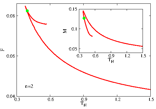
Figure 1: Left panel: The free energy $F=M-T_{H}S$ and the mass $M$ are shown as functions of the Hawking temperature for a set of static axially symmetric black holes in Einstein-scalar field theory with the input parameters $\lambda=-9$, $\mu=0$ and $\alpha=0.1$. Right panel: The horizon excentricity $\epsilon=L_{e}/L_{p}$ is shown as a function of horizon area for the same solutions. Note that in all plots in this work, the quantities are expressed in units of $L$, the cosmological length scale.

Figure 2: The scalar field (left) and the energy density (right) on the horizon are shown for an $n=2$ static axially symmetric black hole in Einstein-scalar field theory marked with a green dot in Figure 1.

However, as we shall argue, the same mechanism holds for the more general scalar Ansatz (3.4). In this work we consider a simple potential allowing for $U<0$,

$$U=\mu^{2}|\Phi|^{2}-\lambda|\Phi|^{4},$$ (3.5)

where $\lambda$ is a strictly positive parameter and $\mu$ is the scalar field mass. The constants $\mu$ and $L$ fix the behaviour of the scalar field as $r\to\infty$, with

$$Z\sim\frac{c_{+}(\theta)}{r^{\Delta_{+}}}+\frac{c_{-}(\theta)}{r^{\Delta_{-}}},~{}{\rm with}~{}~{}\Delta_{\pm}=\frac{3}{2}\left(1\pm\sqrt{1+\frac{4}{9}\mu^{2}L^{2}}\right),$$ (3.6)

$c_{\pm}(\theta)$ being two functions that label the different boundary conditions.

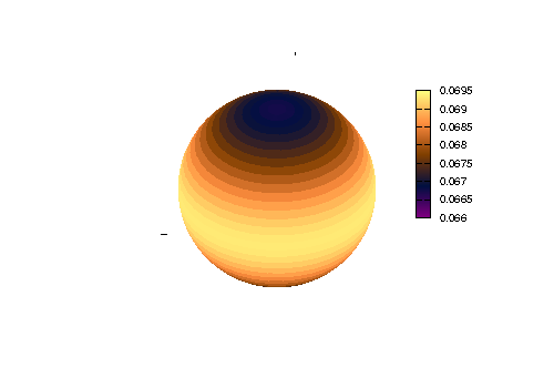
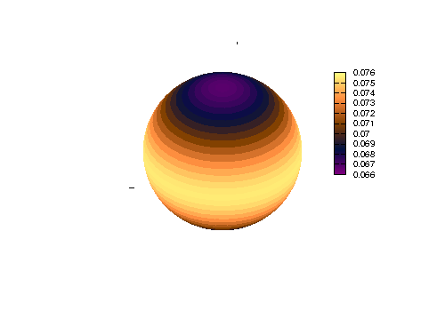
Figure 3: The $<\tau_{\theta}^{\theta}>$ (left) and $<\tau_{\varphi}^{\varphi}>$ (right) components of the holographic stress tensor are shown for the solution in Fig. 2.

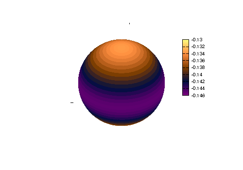
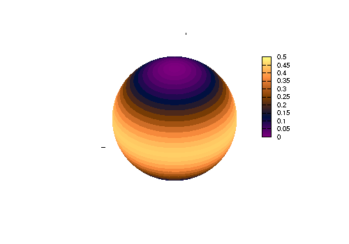
Figure 4: The $<\tau_{t}^{t}>$ component of the holographic stress tensor (left) and the function $c_{+}(\theta)$ which enters the asymptotics (3.6) (right) are shown for the Einstein-scalar field solution in Fig. 2.

3.1.2 The results

The recent work [9] has shown the existence of both BH and soliton solutions of this model for the $\Lambda=0$ limiting case, for the same scalar potential (3.5).

As expected, those configurations survive in the presence of a negative cosmological constant. The discussion in this case should start with the observation that the eq. (3.2) possesses solutions already in the probe limit, $i.e.$ when neglecting the backreaction on the spacetime geometry. This case is discussed in Appendix A1, where we give numerical arguments for the existence of $n>0$ finite mass, regular solutions of the (nonlinear) Klein-Gordon eq. (3.2) in the background of a SAdS BH. There we notice first the existence of a non-trivial zero horizon size limit, which describes a static, non-spherically symmetric soliton in a fixed AdS background. Second, the solutions do not exist for arbitrarly large SAdS BHs, with the emergence of a critical horizon radius and a secondary branch extending backwards in $r_{H}$.

As expected, these solutions survive when taking into account the backreaction on the spacetime geometry. In the numerics, we scale $Z\to Z/L$; moreover, to simplify the problem, we consider the case $\mu=0$ only. Then the system possesses an extra scaling symmetry $r\to rc$, $L\to Lc$ and $\lambda\to\lambda/c^{2}$ (with $c>0$ an arbitrary constant) which can be used to fix the value of $\lambda$ in (3.5). Also, for all solutions, the scalar field is invariant under a reflection in the equatorial plane. Finally, we impose $c_{-}=0$ in the asymptotic expression (3.6) such that the scalar field decays as $1/r^{3}$ as $r\to\infty$.

In Figure 1 we give some results of the numerical integration for a set of $n=2$ solutions with $\Lambda=-3$, $\lambda=-9$, $\mu=0$ and $\alpha=0.1$. In the numerics, the control parameter is $r_{H}$ which fixes the size of the event horizon, with $A_{H}\to 0$ and $T_{H}\to\infty$ as $r_{H}\to 0$, a limit which corresponds to a gravitating scalar soliton. As $r_{H}$ increases, both the mass and the event horizon area increase while the temperature decreases.

These BHs cannot be arbitrarly large, and we notice the emergence of a secondary branch of BHs for a critical configuration, extending backward in $r_{H}$, towards $r_{H}\to 0$. However, the numerics becomes increasingly challenging on the 2nd branch and clarifying this limiting behaviour remains a task beyond the purposes of this paper. Here we only note that the solutions on the first branch minimize the free energy $F=M-T_{H}S$ and are thermodynamically favoured.

An interesting feature of the solutions studied so far is that they always possess an oblate horizon, $\epsilon=L_{e}/L_{p}>1$, as seen in Figure 1 (right) (although the deviation from sphericity is rather small). Also, both the scalar field $Z$ and the energy density $\rho=-T_{t}^{t}$ do not vanish on the horizon, possessing a strong angular dependence, as seen in Figure 2. The shape of the scalar field and the energy density in the bulk are rather similar to those shown in Appendix A1 for the probe limit, and we shall not display them here.

As seen in Figures 3, 4, the deviation from sphericity of the bulk reflects itself in the holographic stress tensor $<\tau_{i}^{j}>$. One can see that as expected $<\tau_{t}^{t}>$ is negative, while, in contrast to the spherically symmetric case, $<\tau_{\theta}^{\theta}>\neq<\tau_{\varphi}^{\varphi}>$. Moreover, the function $c_{+}(\theta)$ which enters the asymptotics (3.6) of the scalar field possesses also a strong $\theta$-dependence, as seen in Figure 4 (right).

3.2 Einstein–Yang-Mills solutions

3.2.1 The model

In order to test the generality of the results above, it is necessary to consider static axially symmetric BHs with other matter fields. For $\Lambda=0$, the first (and still the best known) example of such solutions has been found in a model with Yang-Mills-SU(2) gauge fields [8]. In this case, the matter Lagrangean reads

$${\cal L}_{m}=-\frac{1}{2}{\rm Tr}\big{\{}F_{\mu\nu}F^{\mu\nu}\big{\}},$$ (3.7)

with the field strength tensor

$$F_{\mu\nu}=\partial_{\mu}A_{\nu}-\partial_{\nu}A_{\mu}+i[A_{\mu},A_{\nu}]\ ,$$ (3.8)

and the gauge potential

$$A_{\mu}=\frac{1}{2}\tau_{a}A_{\mu}^{a},$$ (3.9)

$\tau_{a}$ being SU(2) matrices. Variation of (3.7) with respect to the gauge field $A_{\mu}$ leads to the YM equations

$$\nabla_{\mu}F^{\mu\nu}+i[A_{\mu},F^{\mu\nu}]=0,$$ (3.10)

while the variation with respect to the metric $g_{\mu\nu}$ yields the energy-momentum tensor of the YM fields

$$T_{\mu\nu}^{(YM)}=2{\rm Tr}\big{\{}F_{\mu\alpha}F_{\nu\beta}g^{\alpha\beta}-\frac{1}{4}g_{\mu\nu}F_{\alpha\beta}F^{\alpha\beta}\big{\}}\ .$$ (3.11)

As discussed in Appendix A2, similar to the scalar field case discussed above, the axially symmetric YM Ansatz contains an azimuthal winding number $n$, as seen in eqs. (A.5)-(A.6). This Ansatz is parametrized by four functions $H_{i}(r,\theta)$, the explicit dependence on $\varphi$ being factorized in the expression of the SU(2) basis, such that, in the chosen gauge, $\partial/\partial\varphi$ is not a Killing vector of the full EYM system. However, similar to the scalar case, the components of the energy-momentum tensor depend on $(r,\theta)$ only.

A fundamental solution here is the (embedded-U(1)) Reissner-Nordström-anti-de Sitter (RNAdS) BH, which has vanishing potentials, $H_{i}=0$ and a net magnetic charge $Q_{M}=n$. Apart from that, there are also genuine non-Abelian BHs, which in the simplest case are spherically symmetric, with $n=1$ and nontrivial potentials $H_{2}=H_{4}=w(r)$ while $H_{1}=H_{3}=0$. Different from the (embedded) Abelian case, these configurations may carry a zero net magnetic charge, $Q_{M}=0$. An overview of their properties is given in [26] for $\Lambda=0$. An interesting supersymmetric extension of these solutions can be found in [27].

As discussed in [8], the $\Lambda=0$ BHs possess static axially symmetric generalizations, which are found by taking a value $n>1$ for the azimuthal winding number in the YM ansatz (A.5). They possess an event horizon of spherical topology, which, however, is not a round sphere, and approach asymptotically a Minkowski spacetime background. These results have been generalized in [30] by a YM Ansatz containing a further integer, $m>0$, related to the polar angle $\theta$. In the present formulation of the problem, this integer enters the boundary conditions at infinity of the gauge potentials, as seen in eqs. (A.9) and (A.10).

3.2.2 The results

We have found that all known $\Lambda=0$ static axially symmetric EYM BHs possess generalizations with AdS asymptotics. Moreover, new sets of configurations without asymptotically flat counterparts do also occur. The existence of the new solutions can be traced back to the peculiar properties of the YM system in AdS spacetime. In this case, the confining properties of the AdS geometry (effectively) play the role of a Higgs field, leading to a much richer set of possible boundary conditions at infinity, as compared to the case $\Lambda=0$. These boundary conditions are given in Appendix A2, where we provide an overview of the axially symmetric solutions of the YM equations in a SAdS background, for several values of the integers $(m,n)$ introduced above. Note that for an (S)AdS background, the boundary conditions satisfied by the YM potentials at infinity contain an extra-parameter $w_{0}$, which fixes the magnetic charge, as seen in eq. (A.11). This parameter is not fixed apriori, such that YM solutions with a non-integer magnetic charge are allowed [28, 29, 23].

As expected, these YM configurations survive when taking into account the backreaction on the spacetime geometry. The boundary conditions satisfied by the gauge potentials $H_{i}$ at infinity, on the horizon and on the symmetry axis are similar to those used in the probe limit, as stated in Appendix A2.

An interesting feature shared by all EYM axially symmetric BHs studied so far, is that in contrast to the solutions with a scalar field, they possess a prolate horizon, $\epsilon=L_{e}/L_{p}<1$, although the horizon’s deviation from sphericity remains small, as seen in Figure 5 (left). However, as shown in Figures 5, 8 (right panels), the holographic stress tensor exhibits a strong $\theta$-dependence, with $<\tau_{t}^{t}>$ always strictly negative. Also, the energy density shows a strong angular dependence, as seen in Figure 6; in particular its value on the horizon varies with $\theta$.

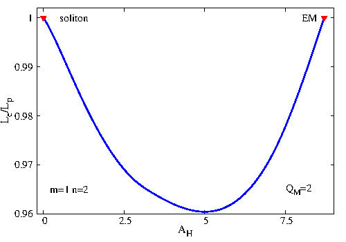
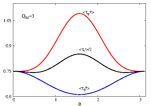
Figure 5: Left panel: The ratio $L_{e}/L_{p}$ (which gives a measure of the horizon deformation) is shown as a function of the horizon area for a set of $m=1,~{}n=2$ Einstein–Yang-Mills (EYM) solutions with $\alpha=0.5$ and magnetic charge $Q_{M}=2$. These configurations interpolate between a horizonless EYM soliton and a critical Reissner-Nordström-AdS black hole, see Figure 7 (left). Right panel: The holographic stress tensor is shown for a typical EYM static axially symmetric solution with the input parameters $m=1,n=3$, $\alpha=0.5$, $r_{H}=0.4$ and $Q_{M}=3$.

Figure 6: The energy density is shown for typical $m=1$ (left) and $m=3$ (right) static axially symmetric solutions with vanishing net magnetic charge in Einstein–Yang-Mills theory. The $m=1$ solution has the input parameters $n=2$, $\alpha=0.15$ and $r_{H}=0.05$, while the one with $m=3$ has $n=1$, $\alpha=0.1$ and $r_{H}=0.05$. The axes here are $\rho=\bar{r}\sin\theta$, $z=\bar{r}\cos\theta$, with $\bar{r}=\sqrt{r^{2}+r_{H}^{2}}$.

Concerning further properties of the solutions, the results can be summarized as follows. First, we have found that all YM configurations in a fixed SAdS background possess gravitating generalizations. The backreaction is taken into account by slowly increasing the value of the parameter $\alpha=\sqrt{4\pi G}/{L}$. As the coupling constant $\alpha$ increases, the spacetime geometry is more and more deformed. However, $\alpha$ cannot be arbitrarily large. The solutions stop to exist at a critical value which, for a given $Q_{M}$, depends on both integers $(m,n)$ and on the size of the horizon, as specified by $r_{H}$. There, a second branch of solutions emerges, which extends backward towards $\alpha\to 0$. Indeed, this limit can be approached in two ways: (i) for the Newton constant $G\to 0$, or, (ii) for $L\to\infty$ (or, equivalently, $\Lambda\to 0$). In the former case one recovers the YM solutions in a fixed SAdS background, while the latter case (with $Q_{M}=0$) corresponds to the known EYM hairy BH in the asymptotically flat spacetime [8, 30]. In contrast, the configurations with $Q_{M}\neq 0$ do not possess a well-defined asymptotically flat limit.

Second, all configurations possess a nontrivial horizonless, particle-like limit, which is approached as the horizon size shrinks to zero. The corresponding solitonic solutions have been extensively studied in [23] (and their asymptotically flat counterparts in [33, 30]). The most interesting feature found there is the existence for $m>1$ of balanced, regular composite configurations, with several distinct components. Our results show that, as expected, all these solutions survive when including a horizon at their center of symmetry.

Figure 7: The free energy $F=M-T_{H}S$ is shown as a function of the Hawking temperature for several sets of static axially symmetric black holes in Einstein–Yang-Mills (EYM) theory, together with the Einstein-Maxwell (EM) solutions with the same magnetic charge. These solutions possess a net magnetic charge $Q_{M}=n$.

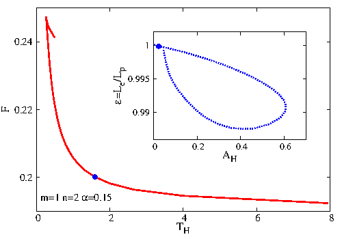
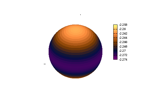
Figure 8: Left panel: The free energy $F=M-T_{H}S$ is shown as a function of the Hawking temperature for a set of Einstein–Yang-Mills static axially symmetric black holes with a vanishing net magnetic charge, $Q_{M}=0$. The inset shows the ratio $L_{e}/L_{p}$ (which gives a measure of the horizon deformation) as a function of horizon area for the same set of black holes. Right panel: The $<\tau_{t}^{t}>$ component of the holographic stress tensor is shown for a solution marked with a dot on the left panel.

In our study we have paid special attention to (possibly) the most interesting case, corresponding to configurations whose YM far field asymptotics describe a gauge transformed charge$-n$ Abelian (multi)monopole. Then, to leading order, the far field asymptotics of the EYM solutions are identical to those of an embedded RNAdS BH with a magnetic charge $Q_{M}=n$.

These solutions have a number of interesting thermodynamical features, whose systematic study is, however, beyond the purposes of this work. Here we mention only that the existing results suggest that the picture found in [35] for $m=n=1$ spherically symmetric solutions can be generalized to the axially symmetric case. That is, for a given $\alpha$, the branches of solutions possessing a net integer magnetic charge bifurcate from some critical RNAdS configuration with the same $(Q_{M},\alpha)$. Also, for all configurations, there exists an (embedded-Abelian) charge$-n$ RNAdS solution which is thermodynamically favoured over the non-Abelian ones, as seen in Figure 7.

We have studied also several sets of $m=1$ and $m=3$ solutions with a vanishing net magnetic flux $Q_{M}=0$. (Note, however, that the bulk magnetic charge density is nonzero.) The simplest solutions here have $m=1,n=1$, being spherically symmetric [28, 29]. (These configurations can be considered as the natural counterparts of the $\Lambda=0$ EYM BHs [26].) Axially symmetric generalizations of the $m=1$ BHs are found by taking $n\geq 2$ in the YM ansatz (A.5). The configurations with $m=3$ do not possess a spherically symmetric limit. Some of the basic properties of these solutions are different as compared to the case with a net magnetic charge $Q_{M}\neq 0$ above. For example, they do not emerge as perturbations of an embedded Abelian solution. Then the geometry of the (zero charge) SAdS BH is approached (to leading orders) in the asymptotic region only. The thermodynamics of the solutions is also different as compared to the magnetically charged case, our results suggesting that the picture found in the recent work [35] for $m=1,n=1$ BHs remains valid in the axially symmetric case. For example, in a free energy-temperature diagram, one finds two branches of solutions, which form a cusp for some minimal value of $T_{H}$, as seen in Figure 8 (left panel).

Finally, let us also mention the existence of configurations with a non-integer (and non-vanishing) magnetic charge. Although we did not attempt to investigate these solutions in a systematic way, we confirm that such EYM BHs also possess a prolate event horizon.

4 Further remarks. Static axially symmetric black holes in Einstein-Maxwell-AdS theory?

The main purpose of this paper was to show the existence of asymptotically AdS₄ static BHs which are axially symmetric only. As explicit examples, we have considered first the case of Einstein-(complex) scalar field theory, followed by a study of static axially symmetric BHs in Einstein–Yang-Mills theory.

In both cases the mechanism which allowed for the existence of such BHs was the symmetry non-inheritance of the matter fields [7]. That is, the matter fields possess a dependence on the azimuthal angle $\varphi$, which, however, does not manifest at the level of the energy-momentum tensor. Similar solutions should exist in various other models with this feature, $e.g.$ Einstein-Skyrme or Einstein–Yang-Mills–Higgs.

There are a number of common features for both types of solutions discussed in this work. For example, they possess a smooth particle-like horizonless limit; as such, both classes of BHs follow the paradigm of ‘event horizons inside classical lumps’ [36]. They can also be considered as ‘bound states of an ordinary black hole and a soliton’ [37]. Moreover, the size of such BHs cannot be arbitrarily large, with the occurrence of a secondary branch of solutions for a critical configuration which maximizes the horizon area. We also note that some of their basic features can be derived based on the results obtained in the probe limit ($i.e.$ matter field(s) in a fixed BH background).

Perhaps the most unexpected feature of the solutions in this work is that the excentricity of the horizon (as measured by $\epsilon=L_{e}/L_{p}$), changes from oblate to prolate when considering BHs in Einstein–scalar field theory and EYM theory. Thus, the internal (matter field(s)) interactions lead to a different shape of the horizon. A better understanding of this feature will require a study of static axially symmetric solutions with a more general matter content. In particular, it will be interesting to consider systems containing gauged scalars. Let us also mention that this kind of configurations (including those in this work) should allow for spinning generalizations, which would possess a single $helical$ Killing vector.

Another possible direction would be the construction of static solitons and BHs with AdS asymptotics, which possess discrete symmetries only. The existence of such solutions is suggested by the results in the literature obtained for a Minkowski spacetime background, the case of Einstein-Skyrme theory being possibly the simplest example [41].(A different example is given in [42].)

One interesting question to ask here is whether the symmetry non-inheritance of the matter fields is the only mechanism leading to static BHs which are axially symmetric only. As argued below, the answer to this question is likely to be negative. For this purpose, in the remainder of this Section, we now discuss the possible existence of static axially symmetric BH solutions in Einstein-Maxwell (EM) theory. Different from the cases in Section 3, the matter field ($i.e.$ the U(1) potential) inherits the spacetime symmetries. Then the possible existence of such EM configurations would be anchored this time in the confining properties of the AdS spacetime.

The starting point here is the study of a more general asymptotical behavior of the YM fields in an AdS background as compared to the one considered in Appendix A2. Another hint comes from the results in the recent paper [43]. There it was shown that the Maxwell equations in a fixed AdS background possess everywhere regular solutions, with finite energy, for every electric multipole moment except for the monopole. Let us briefly review this result. It is well-known that a static axially symmetric charge distribution in a flat spacetime background possesses a multipolar expansion for the electrostatic potential of the form

$$V(r,\theta)=\sum_{\ell\geq 0}R_{\ell}(r)\mathcal{P}_{\ell}(\cos\theta),~{}{\rm with}~{}~{}R_{\ell}(r)=c_{1}R_{\ell}^{(1)}(r)+c_{2}R_{\ell}^{(2)}(r),~{}{\rm and}~{}R_{\ell}^{(1)}(r)=r^{\ell},~{}~{}R_{\ell}^{(2)}(r)=\frac{1}{r^{\ell+1}},~{}$$ (4.1)

(with $c_{1}$, $c_{2}$ arbitrary constants and $\mathcal{P}_{\ell}$ the Legendre polynomial of degree $\ell$) such that any solution diverges either at $r=0$ or for $r\to\infty$. However, as explicitly shown in [43], the situation is different for an AdS background, which regularizes the (far field) divergence in $R_{\ell}^{(1)}(r)$ (with $\ell\geq 1$), which now approaches a constant value as $r\to\infty$. As usual, the existence of such solutions in the probe limit is taken as a strong indication that the full Einstein-Maxwell system possess nontrivial gravitating configurations. Indeed, Ref. [43] has computed the first order perturbation induced in the AdS geometry by a regular electric dipole and found an exact solution showing that all metric functions remain smooth.

However, some of the results in [43] hold also when replacing the AdS background with a SAdS BH. Starting again with a general axially symmetric electrostatic potential $V(r,\theta)=\sum_{\ell\geq 0}R_{\ell}(r)\mathcal{P}_{\ell}(\cos\theta)$, we show in the Appendix A3 that for $\ell\geq 1$ and given $r_{H}\geq 0$, the Maxwell equations possess a solution which is smooth, with finite energy. Unfortunately, this solution cannot be found in closed form (except for $r_{H}=0$ $i.e.$ a globally AdS background); however, it can easily be constructed numerically.

We expect these configurations to survive when including the backreaction on the spacetime geometry (as seen in this work, this was the case for both scalar and YM fields). Thus it is natural to conjecture that ‘the Reissner-Nordström-AdS solution is not the unique static BH in Einstein-Maxwell theory with a negative cosmological constant, with the existence of a different type of AdS BHs which are static and axially symmetric only’.

Acknowledgements.–  We would like to thank C. Herdeiro and B. Kleihaus for relevant discussions. We gratefully acknowledge support by the DFG Research Training Group 1620 ‘Models of Gravity’, by the Alexander von Humboldt Foundation in the framework of the Institutes Linkage Programme, and by FP7, Marie Curie Actions, People, International Research Staff Exchange Scheme (IRSES-606096). E.R. gratefully acknowledges support from the FCT-IF programme.

Appendix A The probe limit

In this Appendix we consider static solutions for several different models in a SAdS background given by

$$ds^{2}=\frac{d\bar{r}^{2}}{N(\bar{r})}+\bar{r}^{2}(d\theta^{2}+\sin^{2}\theta d\varphi^{2})-N(\bar{r})dt^{2},$$ (A.1)

where

$$N(\bar{r})=\left(1-\frac{r_{H}}{\bar{r}}\right)\left(1+\frac{\bar{r}^{2}}{L^{2}}+\frac{r_{H}(r_{H}+\bar{r})}{L^{2}}\right).$$ (A.2)

This geometry possesses a (non-extremal) event horizon at $\bar{r}=r_{H}>0$, the BH mass being $M=\frac{r_{H}}{2}(1+\frac{r^{2}_{H}}{L^{2}})$.

The energy density of a given field configuration, $\rho$, as measured by a static observer with 4-velocity $U^{\mu}\propto\delta^{\mu}_{t}$, is $\rho=-T_{t}^{t}$. The corresponding total mass-energy of the solutions is

$$M=-\int d^{3}x\sqrt{-g}\,T_{t}^{t}=-2\pi\int_{r_{H}}^{\infty}d\bar{r}\int_{0}^{\pi}d\theta~{}\sin\theta~{}\bar{r}^{2}T_{t}^{t}.$$ (A.3)

We solve the matter field equations in the region outside the event horizon only, $\bar{r}\geq r_{H}$. In our numerical approach for both scalar and Yang-Mills fields, a new radial coordinate is introduced, $r=\sqrt{\bar{r}^{2}-r_{H}^{2}}$, with $0\leq r<\infty$, such that the horizon is located at $r=0$. This leads to a simple near horizon expression of the matter fields and, subsequently, to a simple set of boundary conditions there, which are Neumann or Dirichlet only.

A.1 The scalar field in a SAdS background

The matter Lagrangean and the scalar field ansatz are given in Section 3.1, by the relations (3.1) and (3.4), respectively, with $\Phi=Z(r,\theta)e^{in\varphi}$ and $n=1,2,\dots$. The scalar amplitude $Z$ satisfies the following boundary conditions:

$$\partial_{r}Z|_{r=0}=0,~{}~{}Z|_{r=\infty}=0,~{}~{}Z|_{\theta=0,\pi}=0.$$ (A.4)

Figure 9: The mass (divided by the winding number $n$) of the static axially symmetric scalar bound states in a Schwarzschild-AdS background is shown as a function of the event horizon radius.

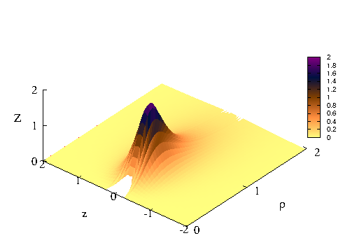
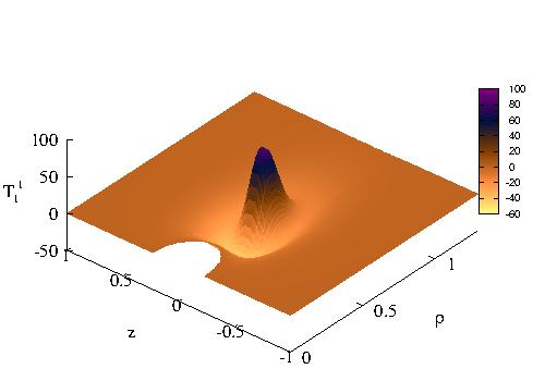
Figure 10: The profile of the scalar field amplitude $Z$ and the $T_{t}^{t}$ component of the energy-momentum tensor are shown for an $n=2$ solution of the non-linear Klein-Gordon equation in a Schwarzschild-AdS background (A.1) with $r_{H}=0.23$, $L=1$. The axes here are $\rho=\bar{r}\sin\theta$, $z=\bar{r}\cos\theta$.

The results of the numerical integration of the nonlinear KG equation (3.2) are shown in Figure 9. (All results in this Subsection have the parameters in the scalar potential $\mu=0$, $\lambda=10$.) Here we exhibit the total mass $vs.$ the horizon size as given by the parameter $r_{H}$, for several values of the winding number $n$. One can notice the existence of two branches of solutions, which form a cusp for some critical $r_{H}$, whose value increases with $n$. The first branch of solutions emerges from the solitonic configurations (which have $r_{H}=0$, $i.e.$ an AdS background). The total mass-energy of the second branch of solutions appears to diverge as $r_{H}\to 0$. A typical solution is shown in Figure 10, where we display both the scalar amplitude $Z$ and the energy density.

A.2 The YM fields in a SAdS background

The YM model has been introduced in Section 3.2, see the relations (3.7)-(3.11). The corresponding axially symmetric Ansatz is more complicated as compared to the scalar field case, and we shall briefly discuss it here. Following the work [8], we choose a gauge potential $A$ containing four gauge field functions $H_{i}$ which depend on $r$ and $\theta$ only; however, it depends also on the azimuthal coordinate $\varphi$, with

$$A_{\mu}dx^{\mu}=\left(\frac{H_{1}}{r}dr+(1-H_{2})d\theta\right)\frac{u_{\varphi}^{(n)}}{2}-n\sin\theta\left(H_{3}\frac{u_{r}^{(n)}}{2}+(1-H_{4})\frac{u_{\theta}^{(n)}}{2}\right)d\varphi.$$ (A.5)

$u_{a}^{(n)}$ are SU(2) matrices which factorize the dependence on the azimuthal coordinate $\varphi$, with

$$u_{r}^{(n)} = \sin\theta(\cos n\varphi~{}\tau_{x}+\sin n\varphi~{}\tau_{y})+\cos\theta~{}\tau_{z},$$

$$u_{\theta}^{(n)} = \cos\theta(\cos n\varphi~{}\tau_{x}+\sin n\varphi~{}\tau_{y})-\sin\theta~{}\tau_{z},$$ (A.6)

$$u_{\varphi}^{(n)} = -\sin n\varphi~{}\tau_{x}+\cos n\varphi~{}\tau_{y},$$

where $\tau_{x},\tau_{y},\tau_{z}$ are the Pauli matrices. The positive integer $n$ represents the azimuthal winding number of the solutions. This ansatz is axially symmetric in the sense that a rotation around the symmetry axis can be compensated by a gauge rotation, $\partial_{\varphi}A_{\mu}=D_{\mu}\bar{\Psi}$ [44, 45, 46], with $\bar{\Psi}$ being a Lie-algebra valued gauge function and $D_{\mu}$ the gauge covariant derivative. The corresponding expression of the field strength tensor can be found $e.g.$ in Ref. [23]. (Note that $F_{\mu\nu}$ also depends on $\varphi$.)

As usually, in order to fix the residual $U(1)$ gauge invariance of the Ansatz (A.5), we impose the gauge fixing condition $r\partial_{r}H_{1}-\partial_{\theta}H_{2}=0$ [8].

Figure 11: The mass-energy $M$ is shown as a function of the horizon radius $r_{H}$ for different sets of YM solutions in a Schwarzschild-AdS background.

The magnetic potentials $H_{i}(r,\theta)$ satisfy a suitable set of boundary conditions at the horizon, at infinity and on the symmetry axis imposed by finite energy, regularity and symmetry requirements. At the horizon ($r=0$) we impose

$$H_{1}|_{r=0}=\partial_{r}H_{2}|_{r=0}=\partial_{r}H_{3}|_{r=0}=\partial_{r}H_{4}|_{r=0}=0,$$ (A.7)

while the boundary conditions on the symmetry axis are

$$H_{1}|_{\theta=0,\pi}=H_{3}|_{\theta=0,\pi}=0,~{}~{}\partial_{\theta}H_{2}|_{\theta=0,\pi}=\partial_{\theta}H_{4}|_{\theta=0,\pi}=0.$$ (A.8)

At infinity, the gauge potentials are required to satisfy a set of boundary conditions originally proposed in [23]. The data there contains a new positive integer, $m$, which is interpreted as a polar winding number solutions. Namely, for odd values of $m$, one imposes

$$H_{1}|_{r=\infty}=0,~{}~{}H_{2}|_{r=\infty}=1-m+w_{0},$$

$$H_{3}|_{r=\infty}=\frac{\cos\theta}{\sin\theta}\bigg{(}\cos((m-1)\theta)-1\bigg{)}+w_{0}\sin((m-1)\theta),$$ (A.9)

$$H_{4}|_{r=\infty}=-\frac{\cos\theta}{\sin\theta}\sin((m-1)\theta)+w_{0}\cos((m-1)\theta),$$

while for even values of $m$ one imposes instead

$$H_{1}|_{r=\infty}=0,~{}~{}H_{2}|_{r=\infty}=1-m-w_{0},~{}~{}$$

$$H_{3}|_{r=\infty}=w_{0}\frac{\cos((m-1)\theta)-\cos\theta}{\sin\theta},~{}~{}$$ (A.10)

$$H_{4}|_{r=\infty}=1-w_{0}-w_{0}\frac{\sin((m-1)\theta)}{\sin\theta},$$

The parameter $w_{0}$ which enters the above relations in an arbitrary constant which fixes the magnetic charge of the solutions [23]. One finds

$$Q_{M}=n|1-w_{0}^{2}|~{}~{}{\rm for~{}odd~{}}m,~{}~{}{\rm and}~{}~{}Q_{M}=\frac{mn}{2}|w_{0}(1-w_{0})|~{}~{}{\rm for~{}even~{}}m.$$ (A.11)

Ref. [23] has given an extensive discussion of the YM solutions in a fixed AdS background, within this general framework. As expected, all those solutions can be generalized by replacing the regular origin with a BH horizon. First, we have solved the YM equations for a large set of $(m,n)$ integers and several (fixed) values of the constant $w_{0}$ in (A.9)-(A.10). Some results in this case are shown in Figure 11, where we exhibit the total mass of the solutions as functions of the size of the BH as given by the horizon radius $r_{H}$. One can notice the existence of two branches of solutions. The lower branch starts with the solution in a fixed AdS background and merges for a critical $r_{H}$ with a secondary branch. This secondary branch extends backward in $r_{H}$, the mass increasing with decreasing the horizon radius. Also, we have found that the maximal value of the horizon radius increases with decreasing $|w_{0}|$.

We have also studied, for given sets of $(m,n)$, solutions in a SAdS background with fixed horizon radius and a varying $w_{0}$ in the asymptotic boundary conditions (A.9)-(A.10) ($i.e.$ the magnetic charge). A general feature here is that solutions exist for a limited range of $w_{0}$ only, and possess a rather complicated branch structure. Thus, for a given horizon size, one cannot find YM configurations with an arbitrarily large (non-Abelian) magnetic charge.

A.3 Maxwell field multipoles in SAdS background

The Lagrangean for a Maxwell field reads

$${\cal L}_{m}=-\frac{1}{4}F_{\mu\nu}F^{\mu\nu},$$ (A.12)

where $F_{\mu\nu}=\partial_{\mu}A_{\nu}-\partial_{\nu}A_{\mu}$ is the $U(1)$ field strength. The four-potential $A_{\mu}$ satisfies the Maxwell equations

$$\nabla_{\mu}F^{\mu\nu}=0,$$ (A.13)

with a line element given by (A.1). (Note that in order to simplify the relations we take $\bar{r}\to r$ in what follows.) The corresponding energy-momentum tensor is

$$T_{\mu\nu}=F_{\mu\alpha}F_{\nu\beta}g^{\alpha\beta}-\frac{1}{4}g_{\mu\nu}F^{2}~{}.$$ (A.14)

Following [43], we consider first a purely electric $U(1)$ potential $A$ which possesses axial symmetry only

$$A_{\mu}dx^{\mu}=V(r,\theta)dt=R_{\ell}(r)\mathcal{P}_{\ell}(\cos\theta)dt\ ,$$ (A.15)

where $\mathcal{P}_{\ell}$ is a Legendre polynomial of degree $\ell$, with $\ell=0,1,\dots$.

From (A.13) it follows that the radial function $R_{\ell}(r)$ is a solution of the equation

$$\frac{d}{dr}\left(r^{2}\frac{dR_{\ell}(r)}{dr}\right)=\frac{\ell(\ell+1)}{N(r)}R_{\ell},$$ (A.16)

with $N(r)$ given by (A.2). Unfortunately, this equation cannot be solved in closed form for a SAdS background, except for $\ell=0$, with $R_{0}=c_{0}-c_{1}/r$. However, ( A.16) can easily be solved numerically for any $\ell\geq 1$; one can also construct an approximate solution at the limits of the $r-$interval. The radial function vanishes on the horizon; the solution there can be written as a power series in $(r-r_{H})$, the first terms being

$$R_{\ell}(r)=r_{1}(r-r_{H})+\frac{r_{1}\left((\ell-1)(\ell+2)-\frac{6r_{H}^{2}}{L^{2}}\right)}{2r_{H}(1+\frac{3r_{H}^{2}}{L^{2}})}(r-r_{H})^{2}+O(r-r_{H})^{3},$$ (A.17)

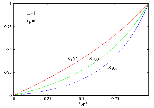
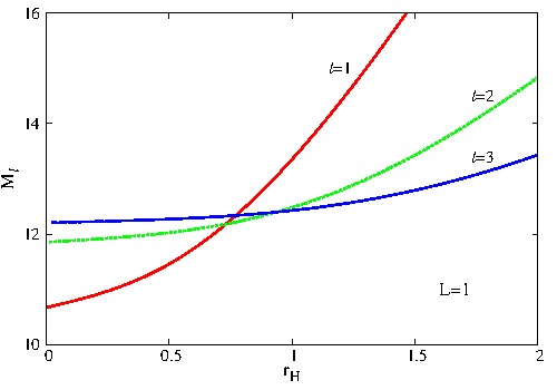
Figure 12: Left panel: The radial function $R_{\ell}$ (with $\ell=1,2,3$) is shown in terms of a compactified coordinate $1-r_{H}/r$ for Maxwell field solutions in a fixed Schwarzschild-AdS background. Right panel: The total mass-energy for families of $\ell=1,2,3$ solutions is shown as a function of the event horizon radius. In both plots, we consider a normalization $R_{\ell}\to 1$ asymptotically.

where $r_{1}$ is a parameter which results from the numerics.

As $r\to\infty$, the solution reads

$$R_{\ell}(r)=1-c_{1}^{(\ell)}\frac{L}{r}+\frac{1}{2}\ell(\ell+1)\frac{L^{2}}{r^{2}}+\dots,$$ (A.18)

where we normalized it such that $R_{\ell}(r)\to 1$ asymptotically. For $r_{H}=0$, one finds $c_{1}^{(\ell)}=\frac{2\Gamma\left(\frac{1+\ell}{2}\right)\Gamma\left(\frac{3+\ell}{2}\right)}{\Gamma\left(1+\frac{\ell}{2}\right)\Gamma\left(\frac{\ell}{2}\right)}$; in a BH background, its value is found numerically.

In Figure 12 (left) we exhibit the radial function $R_{\ell}$ for a SAdS background with a fixed horizon radius $r_{H}=1$ and $\ell=1,2,3$. The dependence of the total mass-energy of the $\ell=1,2,3$ solutions as a function of the event horizon radius is shown in Figure 12 (right). Note that in both plots we take an AdS length scale $L=1$.

Finally, let us mention that given the electric-magnetic duality, for any electric configuration (A.15), one can construct directly the dual magnetic solution. This has (with $\ell>1$):

$$A=\Phi(r,\theta)d\varphi,~{}~{}{\rm with}~{}~{}~{}\Phi_{\ell}(r,\theta)=P_{\ell}(r)U_{\ell}(\theta),$$ (A.19)

where

$$P_{\ell}(r)=r^{2}\frac{dR_{\ell}(r)}{dr},~{}~{}U_{\ell}(\theta)=\sin\theta\frac{d}{d\theta}\mathcal{P}_{\ell}(\cos\theta).$$ (A.20)

References

- [1] P. T. Chrusciel, J. L. Costa and M. Heusler, Living Rev. Rel. 15 (2012) 7 [arXiv:1205.6112 [gr-qc]].
- [2] S. W. Hawking, G. F. R. Ellis, The Large Scale Structure of Space-Time , Cambridge Monographs on Mathematical Physics (1973).
-
[3]
J. L. Friedman, K. Schleich and D. M. Witt,
Phys. Rev. Lett. 71 (1993) 1486
[Phys. Rev. Lett. 75 (1995) 1872]
[gr-qc/9305017];
P. T. Chrusciel and R. M. Wald, Class. Quant. Grav. 11 (1994) L147 [gr-qc/9410004]. -
[4]
R. B. Mann,
Annals Israel Phys. Soc. 13 (1997) 311
[gr-qc/9709039];
L. Vanzo, Phys. Rev. D 56 (1997) 6475 [gr-qc/9705004];
D. Birmingham, Class. Quant. Grav. 16 (1999) 1197 [hep-th/9808032];
R. Aros, R. Troncoso and J. Zanelli, Phys. Rev. D 63 (2001) 084015 [hep-th/0011097]. - [5] J. M. Maldacena, Adv. Theor. Math. Phys. 2 (1998) 231 [Int. J. Theor. Phys. 38 (1999) 1113] [arXiv:hep-th/9711200].
- [6] E. Witten, Adv. Theor. Math. Phys. 2 (1998) 253 [arXiv:hep-th/9802150].
- [7] I. Smolić, Class. Quant. Grav. 32 (2015) 14, 145010 [arXiv:1501.04967 [gr-qc]].
-
[8]
B. Kleihaus and J. Kunz,
Phys. Rev. Lett. 79 (1997) 1595
[gr-qc/9704060];
B. Kleihaus and J. Kunz, Phys. Rev. D 57 (1998) 6138 [gr-qc/9712086]. - [9] B. Kleihaus, J. Kunz, E. Radu and B. Subagyo, Phys. Lett. B 725 (2013) 489 [arXiv:1306.4616 [gr-qc]].
-
[10]
B. Kleihaus and J. Kunz,
Phys. Rev. Lett. 86 (2001) 3704
[gr-qc/0012081];
B. Kleihaus, J. Kunz and F. Navarro-Lerida, Phys. Rev. D 69 (2004) 064028 [gr-qc/0306058]. - [11] O. J. C. Dias, G. T. Horowitz and J. E. Santos, JHEP 1107 (2011) 115 [arXiv:1105.4167 [hep-th]].
- [12] B. Hartmann, B. Kleihaus, J. Kunz and M. List, Phys. Rev. D 82 (2010) 084022 [arXiv:1008.3137 [gr-qc]].
-
[13]
C. A. R. Herdeiro and E. Radu,
Phys. Rev. Lett. 112 (2014) 221101
[arXiv:1403.2757 [gr-qc]];
C. A. R. Herdeiro and E. Radu, Class. Quant. Grav. 32 (2015) 14, 144001 [arXiv:1501.04319 [gr-qc]];
C. A. R. Herdeiro, E. Radu and H. Runarsson, arXiv:1509.02923 [gr-qc]. - [14] B. Kleihaus, J. Kunz and S. Yazadjiev, Phys. Lett. B 744 (2015) 406 [arXiv:1503.01672 [gr-qc]].
- [15] M. Headrick, S. Kitchen and T. Wiseman, Class. Quant. Grav. 27 (2010) 035002 [arXiv:0905.1822 [gr-qc]].
- [16] A. Adam, S. Kitchen and T. Wiseman, Class. Quant. Grav. 29 (2012) 165002 [arXiv:1105.6347 [gr-qc]].
- [17] T. Wiseman, arXiv:1107.5513 [gr-qc].
- [18] O. J. C. Dias, J. E. Santos and B. Way, arXiv:1510.02804 [hep-th].
- [19] V. Balasubramanian and P. Kraus, Commun. Math. Phys. 208 (1999) 413 [arXiv:hep-th/9902121].
- [20] A. Ashtekar and S. Das, Class. Quant. Grav. 17 (2000) L17 [hep-th/9911230].
- [21] S. de Haro, S. N. Solodukhin and K. Skenderis, Commun. Math. Phys. 217 (2001) 595 [hep-th/0002230].
-
[22]
W. Schönauer and R. Weiß,
J. Comput. Appl. Math. 27, 279 (1989) 279;
M. Schauder, R. Weiß and W. Schönauer, The CADSOL Program Package, Universität Karlsruhe, Interner Bericht Nr. 46/92 (1992). - [23] O. Kichakova, J. Kunz, E. Radu and Y. Shnir, Phys. Rev. D 90 (2014) 12, 124012 [arXiv:1409.1894 [gr-qc]].
- [24] E. Radu and B. Subagyo, Phys. Lett. B 717 (2012) 450 [arXiv:1207.3715 [gr-qc]].
-
[25]
T. Hertog and K. Maeda,
JHEP 0407 (2004) 051
[hep-th/0404261];
T. Hertog and K. Maeda, Phys. Rev. D 71 (2005) 024001 [hep-th/0409314];
T. Hertog, AIP Conf. Proc. 743 (2005) 305 [hep-th/0409160];
M. Henneaux, C. Martinez, R. Troncoso and J. Zanelli, Phys. Rev. D 70 (2004) 044034 [hep-th/0404236];
E. Radu and D. H. Tchrakian, Class. Quant. Grav. 22 (2005) 879 [hep-th/0410154]. - [26] M. S. Volkov and D. V. Gal’tsov, Phys. Rept. 319 (1999) 1 [hep-th/9810070].
-
[27]
M. Huebscher, P. Meessen, T. Ortin and S. Vaula,
JHEP 0809 (2008) 099
[arXiv:0806.1477 [hep-th]];
P. Meessen and T. Ortin, JHEP 1504 (2015) 100 [arXiv:1501.02078 [hep-th]]. - [28] E. Winstanley, Class. Quant. Grav. 16 (1999) 1963
- [29] J. Bjoraker and Y. Hosotani, Phys. Rev. D 62 (2000) 043513
- [30] R. Ibadov, B. Kleihaus, J. Kunz and M. Wirschins, Phys. Lett. B 627 (2005) 180 [gr-qc/0507110].
- [31] E. Radu and E. Winstanley, Phys. Rev. D 70 (2004) 084023 [hep-th/0407248].
- [32] R. B. Mann, E. Radu and D. H. Tchrakian, Phys. Rev. D 74 (2006) 064015 [hep-th/0606004].
-
[33]
B. Kleihaus and J. Kunz,
Phys. Rev. Lett. 78 (1997) 2527
[hep-th/9612101];
B. Kleihaus and J. Kunz, Phys. Rev. D 57 (1998) 834 [gr-qc/9707045]. - [34] H. Boutaleb-Joutei, A. Chakrabarti and A. Comtet, Phys. Rev. D 20 (1979) 1884.
- [35] O. Kichakova, J. Kunz, E. Radu and Y. Shnir, Phys. Lett. B 747 (2015) 205 [arXiv:1503.01268 [hep-th]].
-
[36]
D. Kastor and J. H. Traschen,
Phys. Rev. D 46 (1992) 5399
[hep-th/9207070];
C. A. R. Herdeiro and E. Radu, Int. J. Mod. Phys. D 23 (2014) 12, 1442014 [arXiv:1405.3696 [gr-qc]]. -
[37]
A. Ashtekar and B. Krishnan,
Living Rev. Rel. 7 (2004) 10
[gr-qc/0407042];
B. Kleihaus, J. Kunz, A. Sood and M. Wirschins, Phys. Rev. D 65 (2002) 061502 [gr-qc/0110084]. -
[38]
O. Kichakova, J. Kunz and E. Radu,
Phys. Lett. B 728 (2014) 328
[arXiv:1310.5434 [gr-qc]];
O. Kichakova, J. Kunz, E. Radu and Y. Shnir, Phys. Rev. D 86 (2012) 104065;
E. Radu and D. H. Tchrakian, Phys. Rev. D 71 (2005) 064002 [hep-th/0411084]. - [39] B. Hartmann, B. Kleihaus and J. Kunz, Phys. Rev. D 65 (2002) 024027 [hep-th/0108129].
- [40] O. J. C. Dias, J. E. Santos and B. Way, arXiv:1505.04793 [hep-th].
- [41] T. Ioannidou, B. Kleihaus and J. Kunz, Phys. Lett. B 635 (2006) 161 [gr-qc/0601103].
-
[42]
B. Kleihaus, J. Kunz and K. Myklevoll,
Phys. Lett. B 605 (2005) 151
[hep-th/0410238];
B. Kleihaus, J. Kunz and K. Myklevoll, Phys. Lett. B 632 (2006) 333 [hep-th/0509106]. - [43] C. Herdeiro and E. Radu, arXiv:1507.04370 [gr-qc].
- [44] N. S. Manton, Nucl. Phys. B 135 (1978) 319.
- [45] C. Rebbi and P. Rossi, Phys. Rev. D 22 (1980) 2010.
-
[46]
P. Forgacs and N. S. Manton,
Commun. Math. Phys. 72 (1980) 15;
P. G. Bergmann and E. J. Flaherty, J. Math. Phys. 19 (1978) 212.