Real-time simulation of dissipation-driven quantum systems

Abstract:

We set up a real-time path integral to study the evolution of quantum systems driven in real-time completely by the coupling of the system to the environment. For specifically chosen interactions, this can be interpreted as measurements being performed on the system. For a spin-1/2 system, in particular, when the measurement results are averaged over, the resulting sign problem completely disappears, and the system can be simulated with an efficient cluster algorithm.

1 Introduction

The generally established way to study the static properties of large quantum systems is using Monte Carlo methods. However, the notorious ’sign problem’ may arise in cases where the probability sampling over the various stochastically generated configurations have negative (or complex) weights. The particularly exciting branch of theoretical physics dealing with the real-time evolution of large quantum systems, gets excluded from the reach of Monte Carlo methods since the configurations contributing to the real-time path integral have complex weights. Moreover, diagonalizing the Hamiltonian is impossible in practice, due to the exponential growth of the Hilbert space with the system size. Matrix product states provide a basis for simulating the real-time evolution of quantum systems, based on the density matrix renormalization group [1]. They are successful only for gapped 1-D systems for moderate time-intervals [3, 4, 5, 6, 7, 8, 9]. Sign problems also occur in Euclidean time simulations of Quantum Chromodynamics at non-zero baryon chemical potential and the fermionic Hubbard model away from half-filling. Frustrated systems and actions with non-zero topological terms again face the same problem. The different physical origins of the different sign problems suggest that there might not be a unique solution applicable to all the cases [10].

One reason why classical computers have problems to simulate quantum systems - especially in real-time - is because quantum entanglement is not easily representable, let alone computable, as classical information in conventional computers. This already led Feynman to propose the use of specially designed quantum devices to mimic quantum systems [11], very much along the lines of the usage of toy aeroplane models to study actual problems of aircraft manoeuvring in real-time flight situations. This so-called analog computing differs from a digital computer, which is a machine capable of computing an answer to a problem according to an algorithm. Ever since the experimental realization of Bose-Einstein condensation [12, 13], quantum optics has progressed by leaps and bounds, and the degree of control available for ultracold atomic systems is truly remarkable. The bosonic Hubbard model has been implemented with well-controlled ultracold atoms in an optical lattice [14], and several aspects of this quantum simulation have been verified by comparison with accurate quantum Monte Carlo simulations [15]. Digital [16] and analog [17] quantum simulators are widely discussed in atomic and condensed matter physics [18, 19, 20, 21, 22, 23], and more recently also in a particle physics context [24, 25, 26, 27, 28, 29, 30, 31, 32].

However, quantum simulators are not always universally applicable, and even more importantly they are not yet precision instruments. Therefore, the study of real-time evolution of quantum systems using classical computers remains an open important challenge. Closed quantum systems tend to evolve into complicated entangled states under the action of the Hamiltonian in real time rendering their simulation difficult. A different approach is to consider open quantum systems, as they undergo decoherence due to their continuous interaction with the environment.

In this work, we have developed a method to simulate the dynamics of large quantum systems, driven entirely by the measurement process of the total spin $(\vec{S}_{x}+\vec{S}_{y})^{2}$ of pairs of spins $\frac{1}{2}$ at nearest neighbors $x$ and $y$. These measurements can also be interpreted as a dissipative coupling to the environment, especially when this interaction takes place stochastically. As we shall see, the system is driven from a given equilibrium initial state to a new equilibrium final state for late real-times. This is the first example where the real-time evolution of a large strongly coupled quantum system can be studied over arbitrarily large periods of real time in any spatial dimension.

2 Formulation of the problem

To begin with, we outline the path integral representation for the real-time process driven by measurements. Consider a general quantum system with a Hamiltonian, whose evolution in real time from $t_{k}$ to $t_{k+1}$ is described by the operator $U(t_{k+1},t_{k})=U(t_{k},t_{k+1})^{\dagger}$. An observable $O_{k}$ with an eigenvalue $o_{k}$ is measured at time $t_{k}$ ($k\in\{1,2,\dots,N\}$). The measurement projects the state of the system to the subspace of the Hilbert space spanned by the eigenvectors of $O_{k}$ with eigenvalue $o_{k}$, and is represented by the Hermitean operator $P_{o_{k}}$. Starting from an initial density matrix $\rho_{0}=\sum_{i}p_{i}|i\rangle\langle i|$ (with $0\leq p_{i}\leq 1$, $\sum_{i}p_{i}=1$) at time $t_{0}$, the probability to reach a final state $|f\rangle$ at time $t_{f}$, after a sequence of $N$ measurements with results $o_{k}$, is then given by [33]

$$p_{\rho_{0}f}(o_{1},o_{2},\dots,o_{N})=$$ (1)

$$\sum_{i}\langle i|U(t_{0},t_{1})P_{o_{1}}U(t_{1},t_{2})P_{o_{2}}\dots P_{o_{N}}U(t_{N},t_{f})|f\rangle\langle f|U(t_{f},t_{N})P_{o_{N}}\dots P_{o_{2}}U(t_{2},t_{1})P_{o_{1}}U(t_{1},t_{0})|i\rangle p_{i}.$$

In general, matrix elements for both the time-evolution and the projection operators are complex, and cannot be simulated by Monte Carlo methods. However, classical measurements should disentangle the quantum system and reduce the sign problem. For simplicity, we consider systems completely driven by measurements, i. e. $U(t_{k},t_{k+1})={\mathbbm{1}}$. To construct the path integral, we insert $\sum_{n_{k}}|n_{k}\rangle\langle n_{k}|={\mathbbm{1}}$ into the first factor and independently $\sum_{n_{k}^{\prime}}|n_{k}^{\prime}\rangle\langle n_{k}^{\prime}|={\mathbbm{1}}$ into the second factor in eq. (1), at all times $t_{k}$. After some rearranging, we arrive at the following expression for the real-time path integral along the Keldysh contour leading from $t_{0}$ to $t_{f}$ and back [34, 35]:

$$p_{\rho_{0}f}(o_{1},o_{2},\dots,o_{N})=\sum_{i}p_{i}\sum_{n_{1},n_{1}^{\prime}}\dots\sum_{n_{N},n_{N}^{\prime}}\prod_{k=0}^{N}\langle n_{k}n_{k}^{\prime}|P_{o_{k}}\otimes P_{o_{k}}^{*}|n_{k+1}n_{k+1}^{\prime}\rangle.$$ (2)

Here $\langle n_{k}n_{k}^{\prime}|P_{o_{k}}\otimes P_{o_{k}}^{*}|n_{k+1}n_{k+1}^{\prime}\rangle=\langle n_{k}|P_{o_{k}}|n_{k+1}\rangle\langle n_{k}^{\prime}|P_{o_{k}}|n_{k+1}^{\prime}\rangle^{*}$, $\langle n_{0}n_{0}^{\prime}|=\langle ii|$, and $|n_{N+1}n_{N+1}^{\prime}\rangle=|ff\rangle$. Further, if the intermediate measurements are of no interest (as is usually the case for dissipation), we can sum over them to arrive at the following result:

$$p_{\rho_{0}f}=\sum_{o_{1}}\sum_{o_{2}}\dots\sum_{o_{N}}p_{\rho_{0}f}(o_{1},o_{2},\dots,o_{N})=\sum_{i}p_{i}\sum_{n_{1},n_{1}^{\prime}}\dots\sum_{n_{N},n_{N}^{\prime}}\prod_{k=0}^{N}\langle n_{k}n_{k}^{\prime}|\widetilde{P}_{k}|n_{k+1}n_{k+1}^{\prime}\rangle,$$ (3)

A dissipative system continuously interacting with an environment can be described by the Lindblad equation. For the system under consideration, the Lindblad operators [36, 37] $L_{o_{k}}=\sqrt{\varepsilon\gamma}P_{o_{k}}$, obey $(1-\varepsilon\gamma N){\mathbbm{1}}+\sum_{k,o_{k}}L_{o_{k}}^{\dagger}L_{o_{k}}={\mathbbm{1}}$, where $\gamma$ determines the probability of measurements per unit time. The index $k$ now labels the Lindblad operators at any fixed instant of time $t_{k}$. The Lindblad equation is:

$$\partial_{t}\rho=\frac{1}{\varepsilon}\sum_{k,o_{k}}\left(L_{o_{k}}\rho L_{o_{k}}^{\dagger}-\frac{1}{2}L_{o_{k}}^{\dagger}L_{o_{k}}\rho-\frac{1}{2}\rho L_{o_{k}}^{\dagger}L_{o_{k}}\right)=\gamma\sum_{k}(\sum_{o_{k}}P_{o_{k}}\rho P_{o_{k}}-\rho).$$ (4)

The second equation is obtained in the continuous time limit, $\epsilon\to 0$. Based on the Lindblad equation, we can again arrive at a path integral expression similar to the one in eqn. (3).

For illustration, lets consider two spins $\frac{1}{2}$, $\vec{S}_{x}$ and $\vec{S}_{y}$. The total spin $S$ eigenstates $|SS^{3}\rangle$ (with 3-component $S^{3}$) are: $|11\rangle=|\uparrow\uparrow\rangle$, $|10\rangle=\frac{1}{\sqrt{2}}(|\uparrow\downarrow\rangle+|\downarrow\uparrow\rangle)$, $|1-1\rangle=|\downarrow\downarrow\rangle$, and $|00\rangle=\frac{1}{\sqrt{2}}(|\uparrow\downarrow\rangle-|\downarrow\uparrow\rangle)$. The projection operators corresponding to a measurement 1 or 0 of the total spin are then given by $P_{1}=|11\rangle\langle 11|+|10\rangle\langle 10|+|1-1\rangle\langle 1-1|$ and $P_{0}=|00\rangle\langle 00|$, such that

$$P_{1}=\left(\begin{array}[]{cccc}1&0&0&0\\ 0&\frac{1}{2}&\frac{1}{2}&0\\ 0&\frac{1}{2}&\frac{1}{2}&0\\ 0&0&0&1\end{array}\right),\quad P_{0}=\left(\begin{array}[]{cccc}0&0&0&0\\ 0&\frac{1}{2}&-\frac{1}{2}&0\\ 0&-\frac{1}{2}&\frac{1}{2}&0\\ 0&0&0&0\end{array}\right).$$ (5)

Note that the negative entries in $P_{0}$ would give rise to the sign problem in a Monte Carlo simulation. However, when the measurement results are not distinguished, $\widetilde{P}=P_{1}\otimes P_{1}^{*}+P_{0}\otimes P_{0}^{*}$ all the matrix elements of the operator are non-negative. Furthermore, a very efficient loop-cluster algorithm has been designed to simulate the system [39].

3 Simulating a large quantum system in real-time

The above example can be straightforwardly generalized to the case of a large quantum spin system in any dimension. We have implemented this process for a spin $S=\frac{1}{2}$ system on a square lattice of size $L\times L$ with periodic boundary conditions. The measurement process involves the nearest-neighbor spins, and is implemented in four steps. The first step measures all the neighboring spins in the 1-direction, at $x=(x_{1},x_{2})$ and $y=(x_{1}+1,x_{2})$ with even $x_{1}$, simultaneously. The second step looks at the spins at $(x_{1},x_{2})$ and $(x_{1},x_{2}+1)$ with even $x_{2}$. In a third and fourth measurement step, the total spins of pairs with odd $x_{1}$ and $x_{2}$ are measured. This is repeated an arbitrary number of times $M$, such that the total number of measurements is $N=4M$. As a Lindblad process, the exact ordering of the measurement is irrelevant, and the measurements are stochastic. We use the Hamiltonian of the Heisenberg anti-ferromagnet $H=J\sum_{\langle xy\rangle}\vec{S}_{x}\cdot\vec{S}_{y}$, to prepare an initial density matrix $\rho_{0}=\exp(-\beta H)$. A cluster algorithm is used to update the whole system, including both the Euclidean and real-time branches as explained in [39].

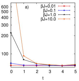
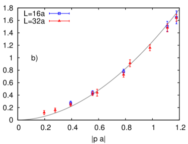
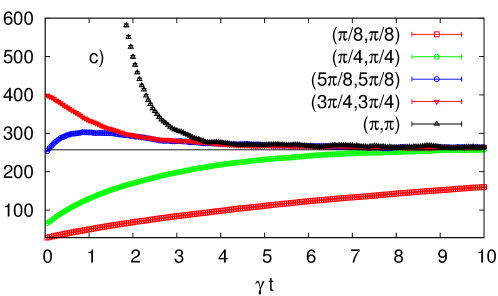
Figure 1: a) Real-time evolution of $\langle M_{s}^{2}\rangle$ driven by discrete measurements, for $\beta J=0.01$, $0.1$, $1$, and $10$, for $L=16a$. b) Inverse equilibration time $1/[\gamma\tau(p)]$ as a function of $|p|$ for $L=16a$, $\beta J=40$, and $L=32a$, $\beta J=80$. c) Evolution of the Fourier modes $\langle|\widetilde{S}(p)|^{2}\rangle$ for the Heisenberg anti-ferromagnet driven by a continuous Lindblad process. The initial ensemble is at a low temperature $\beta J=5L/2a$, where $a$ is the lattice spacing.

At $T=0$, the global $SU(2)$ symmetry of the Heisenberg model is spontaneously broken, and this gives a large signal in the staggered magnetization $M_{s}=\sum_{x}(-1)^{x_{1}+x_{2}}S^{3}_{x}$ of the initial state. Discrete measurements quickly destroy this order, and drive the system to a new steady state as shown in Fig. 1a. A Lindblad process also has the same effect, but since all the spin pairs are not affected simultaneously, the approach to the new steady state happens more slowly, and is dependent on the dissipative coupling strength. The Fourier modes, $\widetilde{S}(p)=\sum_{x}S^{3}_{x}\exp(ip_{1}x_{1}+ip_{2}x_{2})$, $p=(p_{1},p_{2})$, show a similar behavior (Fig. 1c). The symmetry breaking is signalled by a large condensate signal at the Fourier mode $(\pi,\pi)$, and in the nearby modes around this one. The uniform magnetization, $\vec{M}=\sum_{x}\vec{S}_{x}$, on the other hand, is conserved by both the Hamiltonian and the measurement process. Therefore, while the mode $(0,0)$ does not equilibrate at all, the nearby low-momentum modes approach the final state very slowly, according to $\langle|\widetilde{S}(p)|^{2}\rangle\rightarrow A(p)+B(p)\exp(-t/\tau(p))$. For small momenta, the equilibration process is diffusive: $1/[\gamma\tau(p)]=C|pa|^{r}$, $C=1.26(8)$, $r=1.9(2)$ (Fig. 1b).

The dissipation process conserves not only the total spin, but also the lattice translation and rotation symmetries. The final density matrix to which the system is driven, is therefore constrained by these symmetries, and is proportional to the unit matrix in each of these sectors. This can be analytically computed to give $A(p)=L^{4}/(L^{2}-1)$, shown as the horizontal line in Fig. 1c. This is a stable fixed point of the full dynamics (Hamiltonian and the Lindbladian) at $T=\infty$, and acts as a universal attractor for a large class of dissipative process [40].

Another interesting issue is whether a phase transition occurs at a finite instant in real time. While the initial state breaks $SU(2)$ symmetry spontaneously, the final state has a volume independent $\langle M_{s}^{2}\rangle/L^{2}$, indicating a restored $SU(2)$ spin symmetry. This implies that the system passes through a (second-order) phase transition. However, since the Lindblad process takes the system out of thermal equilibrium, this phase transition is not expected to fall into any of the standard dynamic universality classes [41]. To study this, we plot $\langle M_{s}^{2}\rangle/L^{4}$ as well as the Binder ratio $\langle M_{s}^{4}\rangle/\langle M_{s}^{2}\rangle^{2}$ for $\beta J=2L/3a$ in Fig. 2a and 2b. The finite volume curves do not intersect, but their point of inflection moves to later and later real times with increasing spatial volume. The staggered magnetization density ${\cal M}_{s}$, and the length scale $\xi=c/(2\pi\rho_{s})$ (where $c$ is the spin-wave velocity and $\rho_{s}$ is the spin stiffness) are obtained as a function of time, by a fit to the equation

$$\langle M_{s}(t)^{2}\rangle=\frac{{\cal M}_{s}(t)^{2}L^{4}}{3}\sum_{n=0}^{3}c_{n}\left(\frac{\xi(t)}{L}\right)^{n},$$ (6)

which implicitly defines ${\cal M}_{s}(t)$ and $\xi(t)$.The constants $c_{0}=1$, $c_{1}=5.7503(6)$, $c_{2}=16.31(2)$, $c_{3}=-84.8(2)$, accurately determined at $t=0$, are assumed to be time-independent since they are related to the spatial geometry of the system. The exponential decay of the order parameter ${\cal M}_{s}(t)={\cal M}_{s}(0)\exp(-t/\tau)$, (with ${\cal M}_{s}(0)=0.30743(1)/a^{2}$ [42, 43]) suggests that it takes an infinite amount of time for the order to disappear completely and hence for the phase transition to be completed.

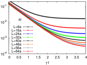
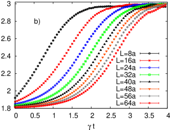
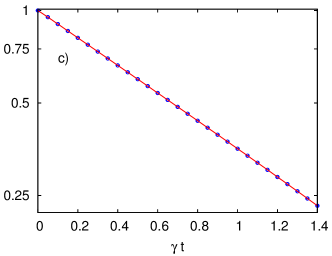
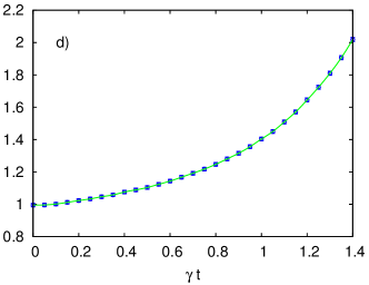
Figure 2: [Color online] a) $\langle M_{s}^{2}\rangle/L^{4}$ and b) Binder ratio $\langle M_{s}^{4}\rangle/\langle M_{s}^{2}\rangle^{2}$ as functions of time for $L/a=12,\dots,48$, $\beta J=8,\dots,30$. Evolution of c) ${\cal M}_{s}(t)/{\cal M}_{s}(0)$ and d) $\xi(t)/\xi(0)$.

4 Conclusion and Outlook

We have demonstrated that for certain measurement or dissipative processes, we can simulate the real-time evolution of a large quantum system on classical computers. The processes under consideration drive initial states (or density matrices) into a new state with only short-range correlations. However, the phase transition into a final disordered steady state without spontaneous symmetry breaking is completed only in an infinite amount of time.

Extending these investigations, we have also studied several other measurement processes and initial states given by the ground states of different models [40]. All these cases show a diffusive behavior of a conserved quantity (i.e., the staggered or the uniform magnetization). Further, the non-equilibrium transport of magnetization in large open systems has also been studied with our method [44]. A study of competing Lindblad processes, and the inclusion of a part of the Hamiltonian along with the dissipation, as well as extension of this formalism to fermionic systems. are currently under investigation.

References

- [1] S. R. White, Phys. Rev. Lett. 68 (1992) 2863.
- [2] U. Schollwöck, Rev. Mod. Phys. 77 (2005) 259.
- [3] G. Vidal, Phys. Rev. Lett. 91 (2003) 147902.
- [4] S. R. White and A. E. Feiguin, Phys. Rev. Lett. 93 (2004) 076401.
- [5] F. Verstraete, I. I. Garcia-Ripoll, and J. I. Cirac, Phys. Rev. Lett. 93 (2004) 207204.
- [6] M. Zwolak and G. Vidal, Phys. Rev. Lett. 93 (2004) 207205.
- [7] A. J. Daley, C. Kollath, U. Schollwöck, and G. Vidal, J. Stat. Mech.: Theor. Exp. P04005 (2004).
- [8] T. Barthel, U. Schollwöck, and S. R. White, Phys. Rev. B79 (2009) 245101.
- [9] I. Pizorn, V. Eisler, S. Andergassen, and M. Troyer, New J. Phys. 16 (2014) 073007.
- [10] M. Troyer and U.-J. Wiese, Phys. Rev. Lett. 94 (2005) 170201.
- [11] R. P. Feynman, Int. J. Theor. Phys. 21 (1982) 467.
- [12] M. H. Anderson et. al., Science 269 (1995) 5221.
- [13] K. B. Davis et. al., Phys. Rev. Lett. 75 (1995) 3969.
- [14] M. Greiner, et al., Nature 415 (2002) 39.
- [15] S. Trotzky et. al., Nature Phys. 6 (2010) 998.
- [16] S. Lloyd, Science 273 (1996) 1073.
- [17] D. Jaksch et. al., Phys. Rev. Lett. 81 (1998) 3108.
- [18] J. I. Cirac and P. Zoller, Nature Phys. 8 (2012) 264.
- [19] M. Lewenstein, A. Sanpera, and V. Ahufinger, “Ultracold Atoms in Optical Lattices: Simulating Quantum Many-Body Systems”, Oxford University Press (2012).
- [20] I. Bloch, J. Dalibard, and S. Nascimbene, Nature Phys. 8 (2012) 267.
- [21] R. Blatt and C. F. Ross, Nature Phys. 8 (2012) 277.
- [22] A. Aspuru-Guzik and P. Walther, Nature Phys. 8 (2012) 285.
- [23] A. A. Houck, H. E. Türeci, and J. Koch, Nature Phys. 8 (2012) 292.
- [24] E. Kapit and E. Mueller, Phys. Rev. A83 (2011) 033625.
- [25] G. Szirmai, E. Szirmai, A. Zamora, and M. Lewenstein, Phys. Rev. A84 (2011) 011611.
- [26] E. Zohar, J. Cirac, and B. Reznik, Phys. Rev. Lett. 109 (2012) 125302.
- [27] D. Banerjee et. al., Phys. Rev. Lett. 109 (2012) 175302.
- [28] D. Banerjee et. al., Phys. Rev. Lett. 110 (2013) 125303.
- [29] E. Zohar, J. Cirac, and B. Reznik, Phys. Rev. Lett. 110 (2013) 125304.
- [30] L. Tagliacozzo et. al., Nature Commun. 4 (2013) 2615.
- [31] L. Tagliacozzo, A. Celi, A. Zamora, and M. Lewenstein, Ann. Phys. 330 (2013) 160.
- [32] U.-J. Wiese, Annalen der Physik 525 (2013) 777.
- [33] R. B. Griffiths, J. Stat. Phys. 36 (1984) 219.
- [34] J. Schwinger, J. Math. Phys. 2 (1961) 407.
- [35] L. V. Keldysh, JETP 47 (1965) 1515.
- [36] A. Kossakowski, Rep. Math. Phys. 3 (1972) 247.
- [37] G. Lindblad, Commun. Math. Phys. 48 (1976) 119.
- [38] K. Kraus, States, Effects and Operations, Fundamental Notions of Quantum Theory, Academic, Berlin (1983).
- [39] D. Banerjee, F. -J. Jiang, M. Kon, and U. -J. Wiese, Phys. Rev. B 90, 241104 (2014).
- [40] F. Hebenstreit et. al., Phys. Rev. B92, 035116 (2015).
- [41] P. C. Hohenberg and B. I. Halperin, Rev. Mod. Phys. 49 (1977) 436.
- [42] A. W. Sandvik and H. G. Evertz, Phys. Rev. B82 (2010) 024407.
- [43] U. Gerber et. al., J. Stat. Mech. (2009) P03021.
- [44] D. Banerjee, F. Hebenstreit, F. -J. Jiang, and U. -J. Wiese, Phys. Rev. B92, 121104 (2015).