Accelerated Magnetic Resonance Thermometry in the Presence of Uncertainties

Abstract

An accelerated model-based information theoretic approach is presented to perform the task of Magnetic Resonance (MR) thermal image reconstruction from a limited number of observed samples on $k-$space. The key idea of the proposed approach is to utilize information theoretic techniques to optimally detect samples of $k-$space that are information rich with respect to a model of the thermal data acquisition. These highly informative $k-$space samples are then used to refine the mathematical model and reconstruct the image. The information theoretic reconstruction is demonstrated retrospectively in data acquired during MR–guided Laser Induced Thermal Therapy (MRgLITT) procedures. The approach demonstrates that locations of high-information content with respect to a model based reconstruction of MR thermometry may be quantitatively identified. The predicted locations of high-information content are sorted and retrospectively extracted from the fully sampled $k-$space measurements data set. The effect of interactively increasing the predicted number of data points used in the subsampled reconstruction is quantified using the L2-norm of the distance between the subsampled and fully sampled reconstruction. Performance of the proposed approach is also compared with clinically available subsampling techniques (rectilinear subsampling and variable-density Poisson disk undersampling). It is shown that the proposed subsampling scheme results in accurate reconstructions using small fraction of $k-$space points and suggest that the reconstruction technique may be useful in improving the efficiency of the thermometry data temporal resolution.

keywords

MRI, thermal ablation, $k-$space, inverse problems, entropy, sensor management, quantification and estimation, Pennes bioheat model.

1 Introduction

Laser Induced Thermal Therapy (LITT) is a non-ionizing and minimally invasive treatment alternative for patients that have reached maximum radiation dose or have surgically unresectable tumors [1, 2, 3, 4, 5, 6]. The approach is being used clinically to rapidly treat focal diseased tissue in liver, prostate, bone, brain, and other types of diseases like epilepsy [7, 8, 9, 10, 11]. MR thermometry is often integrated with the LITT procedure to provide temperature estimates of the target tissue and surrounding critical structures during the laser induced thermal therapy. Currently, MR thermometry is acquired primarily through quantitative phase-sensitive techniques based on the Proton Resonance Frequency (PRF) shift. The information provided by the integrated system, often called MR–guided Laser Thermal Therapy (MRgLITT), improves safety and allows the clinician to reduce power or stop delivery if safety thresholds are exceeded [12].

The idea of combining MR thermometry signals with a mathematical model to better represent the temperature field has been exploited in various works [13, 14, 15]. The essence of all these works is to provide a better estimate of the temperature image based on model–data fusion in a Kalman filtration [16] framework. However, they don’t provide any guidelines about the optimal $k-$space sampling.

This manuscript presents a novel model-based information theoretic approach to increase both the accuracy and efficiency of the thermal image acquisition and reconstruction. The key question is that whether there exist optimal locations on $k-$space such that they provide maximum information regarding the temperature image? And if there exist, how one can develop a general framework to find these locations on $k-$space?

Numerous works have studied the effect of data undersampling on temperature image reconstruction, and image reconstruction in general [17, 18, 19, 20, 21, 22, 23, 24, 25, 26, 27, 28, 29, 30, 31]. Hennig [17] performed a comprehensive study on the effect of rectilinear and non-rectilinear methods for $k-$space sampling. Odeén et al. [26] also performed a comprehensive study on different $k-$space subsampling strategies for MR temperature monitoring in particular. Willinek et al. [18] suggested a randomly segmented central $k-$space ordering for high-spatial-resolution-contrast enhanced MR Angiography. Lustig et al. [19] proposed a sparse sampling technique based on compressed sensing theory [30] to reconstruct MR images from undersampled $k-$space. Vasanawala [31] et al. developed a practical parallel imaging compressed sensing MRI by help of Poisson-disk random undersampling of the phase encode. Majumdar et al. [20] also applied the compressed sensing theory for real time dynamic MR image reconstruction. Performance of compressed sensing in non-convex optimization context for sparse sampling of $k-$space was also studied by Chartrand [22]. Stochastic sampling of $k-$space has also been used in contrast-enhanced MR renography and time-resolved angiography [27, 28, 29]. Todd et al. [21, 25] presented a temporally constrained reconstruction (TCR) algorithm for reconstruction of temperature image from undersampled $k-$space data in an optimization framework.

Model-based reconstruction of temperature data is also recently exploited in few works. Todd et al. [23] provided a model predictive filtering approach for temperature image reconstruction during the MR–guided High Intensity Focus Ultrasound (MRgHIFU). The key idea of this work is to utilize a mathematical model to predict the spatiotemporal variations of temperature, where its parameters are identified based on observed $k-$space data. The identified mathematical model is then combined with a set of under-sampled $k-$space data (by simply replacing the model predictions with observed data) to provide an estimate of temperature image. Geometric techniques were used for under-sampling of $k-$space in this work. Gaur et al. [24] proposed an accelerated MR thermometry approach by model-based estimation of the temperature from undersampled $k-$space. In the heart of this approach, there exists a constrained image model whose parameters are learned from acquired $k-$space data points. The fitted image model is then used to reconstruct artifact-free temperature maps. However, no scheme is provided for selection of $k-$space samples used in finding model parameters.

Information theoretic approaches have also been used in optimal experiment design in MRI and medical imaging in general [32, 33, 34, 35]. The essence of these works lies in finding the optimal experiment parameters based on minimizing Cramer-Rao lower bound. Minimizing Cramer-Rao lower bound provides a reliable technique for finding the optimal parameters of the experiment. However, the major drawback of this technique is that the Fisher information used in Cramer-Rao lower bound can be a function of uncertain parameters. Hence, one needs to use an estimate of the parameters of interest (e.g. prior mean estimate of the parameter) to approximate the Fisher information in Cramer-Rao lower bound, resulting in possible sub-optimalities.

While the majority of work has focused on randomly selected or geometrically undersampled $k-$space points for image reconstruction, herein we tackle the problem of $k-$space under-sampling and temperature image reconstruction from a different perspective. In detail, we first apply an uncertain mathematical model to describe the spatiotemporal evolution of the temperature field and corresponding manifestation of $k-$space measurements. We then apply a general information theoretic framework to identify the most useful locations on $k-$space for data acquisition. Finally, the obtained $k-$space data points are used to refine the mathematical model in reconstructing the temperature image over the tissue.

The key contribution of this article is to provide a general framework to judiciously select the samples on $k-$space such that they result in the best estimate of the corresponding temperature image. This has been achieved by maximizing the entropy of model outputs or maximizing the mutual information [36] between model uncertainties and data observations. Optimally selected observations on $k-$space are then utilized to refine the mathematical model. The refined mathematical model is then used to generate the temperature field corresponding to the observations.

The structure of this paper is as follows: First, mathematical description of the problem is provided in Section 2. Then, we describe the overall picture of the proposed approach in Section 3. In section 4, we discuss the uncertainty quantification for Pennes bioheat equation in presence of parametric uncertainty. The basic idea for optimal $k-$space sampling is then elucidated in Section 5. A brief discussion about the minimum variance framework used for model-data fusion and model based image reconstruction is provided in Sections 6 and 7, respectively. In Section 8, performance of the proposed algorithm is demonstrated using in silico and in vivo examples. Results and discussion conclude the manuscript.

2 Problem Statement

Consider the problem of temperature field estimation during the MRgLITT process. According to the Pennes bioheat equation [37], spatio-temporal behavior of temperature $u(\mathbf{x},t)$ at a given time $t$ and spatial location $\mathbf{x}$ is given by:

$$\raggedright\rho c\frac{\partial u}{\partial t}-\nabla\cdot({\Lambda(u,\mathbf{x})}\nabla u)\@add@raggedright +$$

$${\omega(u,\mathbf{x})}c_{blood}(u-u_{a})=Q_{laser}(\mathbf{x},t),\quad\forall\ \mathbf{x}\in\Omega$$

$$Q_{laser}(\mathbf{x},t)=P(t)\mu^{2}\frac{e^{-\mu||\mathbf{x}-\mathbf{x}_{0}||}}{4\pi||\mathbf{x}-\mathbf{x}_{0}||}$$

$$u(\mathbf{x},0)=u_{0}(\mathbf{x}),\quad\mathbf{x}\in\Omega$$

$$u(\mathbf{x},t)=u_{D}(\mathbf{x}),\quad\mathbf{x}\in\partial\Omega_{D}$$ (1)

$$-\Lambda(u,\mathbf{x})\nabla\cdot u(\mathbf{x},t)=g_{N}(\mathbf{x}),\quad\mathbf{x}\in\partial\Omega_{N}$$

$$-\Lambda(u,\mathbf{x})\nabla\cdot u(\mathbf{x},t)=h(u-u_{\infty}),\quad\mathbf{x}\in\partial\Omega_{c}$$

where, parameters $\rho$ and $c$ are density and specific heat of the tissue, and $\Lambda(u,\mathbf{x}),\ c_{blood}$, and $\omega(u,\mathbf{x})$ represent thermal conductivity, specific heat capacity of blood, and perfusion rate, respectively. Note that $\mathbf{x}$ is an $n-$dimensional spatial domain in general, i.e. $\mathbf{x}\in\mathbb{R}^{n}$. For instance, if $n=2$, then $\Omega$ is a two dimensional domain and $\mathbf{x}=(x,y)$.

$Q_{laser}(\mathbf{x},t)$ denotes the optical-thermal response to the laser source and is modeled as the classical spherically symmetric isotropic solution to the transport equation of light within a laser-irradiated tissue [38]. $P(t)$ is the laser power as a function of time. Parameter $\mathbf{x}_{0}$ denotes the position of laser photon source, and $\mu$ is the optical attenuation coefficient. Note that $\mu$ can be a function of tissue properties in general, i.e. $\mu=\mu(\mathbf{x})$.

The initial temperature of the tissue is denoted by $u_{0}(\mathbf{x})$, which is typically assumed to be $37\ ^{\circ}$C for human body. Also, $u_{D}(\mathbf{x})$ and $g_{N}(\mathbf{x})$ represent Dirichlet and Neumann’s boundary conditions, respectively. Possible effects of blood flow on temperature are also modeled as convection $h(u-u_{\infty})$, where $h$ denotes the convection coefficient and $u_{\infty}$ represents the blood temperature. Note that $u_{\infty}=u_{0}$.

One of the key challenges while using Eq. (1) is that the associated parameters like optical attenuation coefficient $\mu(\mathbf{x})$ are often unknown, and their values are different from patient to patient. Hence, it is a reasonable assumption to treat these parameters as uncertain parameters with some a priori information. Here we will assume the optical attenuation coefficient to be uncertain with some prior probability density function $p(\mu)$. Further, tissue heterogenieties are incorporated using finite spatial variations of the attenuation coefficient:

$$\mu(\mathbf{x})=\sum\limits_{i=1}^{d}\mu_{i}\ U(\mathbf{x}-\Omega_{i})$$ (2)

where, $d$ is the total number of tissue types and $\mu_{i}$ is the corresponding attenuation coefficient for the $i^{th}$ tissue. Note that each of the $\mu_{i}$ is assumed to be uncertain. $\Omega_{i}$ represents the corresponding sub-domain of the $i^{th}$ tissue on spatial domain $\Omega$. Note that $\Omega_{i}$’s are mutually disjoint, i.e.

$$\bigcup_{i=1}^{d}\Omega_{i}=\Omega,\quad\Omega_{i}\cap\Omega_{j}=\varnothing$$

The unitary function $U(.)$ is defined as:

$$U(\mathbf{x}-\Omega_{i})=\begin{cases}1,\quad\mathbf{x}\in\Omega_{i}\\ \\ 0,\quad\text{otherwise}\end{cases}$$ (3)

Hence, the overall optical attenuation coefficient $\mu$ will be a piece-wise continuous function of spatial coordinate $\mathbf{x}$, where the $\mu_{i}$ on each sub-domain $\Omega_{i}$ is considered to be uncertain.

We emphasize here that other parameters of the Pennes bioheat equation (e.g. thermal conductivity, perfusion rate, etc.) can also be uncertain in general. However, for the sake of simplicity, we only considered optical attenuation coefficient, $\mu(\mathbf{x},t)$, to be uncertain in this manuscript. Note that proposed approach in the following can be easily extended to spatio-temporally varying cases with slight modifications.

PRF shift is induced by the fluctuations in the temperature field [39]. We will assume that the changes in the PRF are observed through noise corrupted $k-$space measurements of a steady state gradient echo sequence:

$$z\propto\int_{\Omega}\left(M(\mathbf{x})e^{-s(\mu,\mathbf{x})}\right)e^{-2\pi i\overrightarrow{k}.\mathbf{x}}\;d\mathbf{x}+\nu,\quad\nu\sim\mathcal{N}(0,\sigma)$$ (4)

where, $\overrightarrow{k}=(k_{x},k_{y},k_{z})$ and

$$s(\mu,\mathbf{x})=\frac{T_{E}}{T_{2}^{*}(\mathbf{x})}+i\left\{2\pi\gamma\alpha B_{0}T_{E}\Delta u(\mu,\mathbf{x})+T_{E}\Delta\omega_{0}(\mathbf{x})\right\}$$ (5)

Transverse magnetization $M(x)$ is determined by the repetition time, $T_{R}$, $T_{1}$-relaxation, and flip angle, $\theta$:

$$M(\mathbf{x})=\frac{M_{0}\sin\theta\left(1-e^{-T_{R}/T_{1}}\right)}{\left(1-\cos\theta\ e^{-T_{R}/T_{1}}\right)}$$ (6)

Note that relaxation parameters like $T_{1}$ can be a function of temperature in general. As Eq. (4) represents, observation data is polluted with some normally distributed white noise $\nu$ (with mean 0, and standard deviation $\sigma$). One should note that complex measurement data $z$ is a function of $k-$space parameters $\overrightarrow{k}=(k_{x},k_{y},k_{z})$. Table 1 summarizes the parameters involved in Eq. (4) to Eq. (6).

Table 1: Physical description of the parameters involved in sensor model

Parameter (unit)	Description
$M_{0}$ (Tesla)	equilibrium magnetization
$\theta$ (degree)	Flip Angle (FA)
$T_{1},\ T_{2}^{*}$ (sec)	relaxation parameters
$\Delta\omega_{0}$ (radians)	off-resonance
$T_{E}$ (sec)	echo time
$\gamma$ ($\frac{\text{rad}}{\text{sec.Tesla}}$)	gyromagnetic ratio of water
$\alpha$ ($\frac{\text{ppm}}{{}^{\circ}\text{C}}$)	temperature sensitivity
$B_{0}$ (Tesla)	strength of the magnetic field

To be concise in formulation, one can define the observation model as:

$$\begin{split}z&\propto\mathcal{U}(\mu,\overrightarrow{k})+\nu\qquad\nu\sim\mathcal{N}(0,\sigma)\\ \mathcal{U}(\mu,\overrightarrow{k})&=\int_{\Omega}\left(M(\mathbf{x})e^{-s(\mu,\mathbf{x})}\right)e^{-2\pi i\overrightarrow{k}.\mathbf{x}}d\mathbf{x}\end{split}$$ (7)

Our final goal is to accurately estimate the temperature field over the spatial domain, given a limited number of measurement data $z$. The key challenge to achieve this goal is to find the optimal set of frequencies $(k_{x},k_{y},k_{z})$ such that they provide the maximum amount of information for accurate estimation of uncertain parameter $\mu$ and consequently temperature field $u$.

3 Methodology

The method presented in this paper consists of four different components that are combined together to perform the task of the model-based thermometry image reconstruction. These components consist of i) Uncertainty Quantification (UQ), ii) Optimal $k-$space sampling, iii) Model-Data Fusion, and iv) Model-based Image Reconstruction. Schematic view of the whole estimation process is shown in Fig. 1.

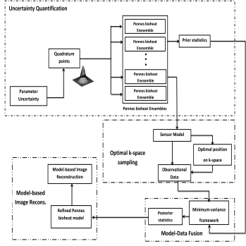
Figure 1: Schematic view of estimation process

As shown in Fig. 1, the process starts with given uncertainties in the parameters of Pennes bioheat equation. The first step to perform the estimation is to quantify the effect of these uncertain parameters on spatio-temporal distribution of the temperature. This is performed by propagation of a set of quadrature points through the Pennes bioheat equation. The weighted average of propagated quadrature points is then used to determine the statistics of the temperature (mean and covariance) over the spatial domain at a given time [2, 40, 41]. Hence, utilizing an appropriate and efficient set of quadrature points is of high importance. The methodology for UQ is discussed in further details in Section 4.

Besides precise quantification of uncertainty, having useful measurement data is also highly important to ensure accurate estimation. This is the focus of this manuscript and is achieved by optimal $k-$space sampling. The key goal of optimal $k-$space sampling is to optimally locate a set of samples over the $k-$space such that the measurement of the most useful data is ensured. This is achieved by maximizing the mutual information between measurements $z$ and model parameters $\mu$. Our approximation to the solution of this problem is presented in Section 5.

To improve our level of confidence about the present uncertainties in the Pennes bioheat equation, prior statistics obtained from UQ and observed data from optimal $k-$space sampling are combined together within a model-data fusion (data assimilation) framework [41]. This will result in posterior statistics (e.g. mean and covariance) of uncertain parameters. Mathematical details of applied data assimilation technique are provided in Section 6.

The obtained posterior statistics are then utilized to refine the parameter values in Pennes bioheat equation, and simulation results provided by this updated mathematical model are used to precisely reconstruct the spread of temperature over the tissue. Detailed description of this process is provided in Section 7.

In here, we should emphasize that the LITT procedure is a dynamic process where the temperature field changes during time. Hence, one would expect the corresponding locations for optimal $k-$space observation to change over the time. However, in this paper we only focus on optimal $k-$space location at a given time step. In fact, temporal change of $k-$space data acquisition points during the LITT procedure is an ongoing subject of research in our group which its result will be published in a separate paper.

4 Uncertainty Quantification

Applying efficient and accurate tools to quantify the uncertainty is necessary for a precise parameter estimation. This can be achieved by different tools ranging from simple Monte Carlo (MC) method to generalized Polynomial Chaos (gPC) [42][43] and the solution of Fokker-Planck-Kolmogorov Equation (FPKE)[44]. The choice of each method for uncertainty quantification depends on the desired level of accuracy and available computational resources.

In here, the method of quadrature points is utilized to perform the task of uncertainty quantification. In the method of quadrature points, a set of intelligently selected points will be propagated through dynamical model and statistics of the output (e.g. mean and variance) are then determined by the weighted average of the model outputs. The major benefit of the quadrature scheme is its significantly less computational cost comparing to Monte Carlo method. Furthermore, the computational complexity involved in quadrature methods is far less than the computational complexities involved in the solution of FPKE and one can easily make use of parallel computing techniques to expedite the procedure. In this paper, due to mentioned benefits of the method of quadrature points with respect to other approaches like MC, gPC, and FPKE, a quadrature based method is being used for quantification of uncertainty in Pennes bioheat equation subjected to parameteric uncertainty.

The method of quadrature points can be viewed as a MC-like evaluation of system of equations, but with sample points selected by quadrature rules. To explain this in more detail, consider $\mu$ to be a time invariant uncertain parameter which can be considered as a function of a random vector $\bm{\xi}=[\xi_{1},\xi_{2},\cdots,\xi_{d}]\in\mathbb{R}^{d}$ defined by a pdf $\textit{p}(\bm{\xi})$ over the support $\Omega_{\xi}$.

In this way, expected value (mean) of temperature at a given spatio-temporal point $(\mathbf{x},t)$ can be written as

$$\hat{u}=\mathcal{E}[u]=\int_{\bm{\xi}}u(\mu,\mathbf{x},t)p(\bm{\xi})d\bm{\xi}\simeq\sum\limits_{q}^{M}w_{q}u(\mu(\bm{\xi}^{q}),\mathbf{x},t)$$ (8)

where, $M$ denotes total number of applied quadrature points and $\mu(\bm{\xi}^{q})$ represents $q^{th}$ quadrature point, generated based on the applied quadrature scheme. Similarly, $j^{th}$ order central moments of temperature at each point $(\mathbf{x},t)$ can be formulated as

$$\mathcal{E}[(u-\hat{u})^{j}]=\int_{\bm{\xi}}(u(\mu,\mathbf{x},t)-\hat{u})^{j}\ p(\bm{\xi})d\bm{\xi}\simeq$$

$$\sum\limits_{q}^{M}w_{q}\left(u(\mu(\bm{\xi}^{q}),\mathbf{x},t)-\hat{u}\right)^{j},\quad j=2,3,\cdots$$ (9)

One can also find moments of $\mathcal{U}$ in similar way, i.e.

$$m_{1}=\hat{\mathcal{U}}=\mathcal{E}[\mathcal{U}]=\int_{\bm{\xi}}\mathcal{U}(\mu,\mathbf{x},t)\ p(\bm{\xi})d\bm{\xi}\simeq$$

$$\sum\limits_{q}^{M}w_{q}\ \mathcal{U}(\mu(\bm{\xi}^{q}),\mathbf{x},t)$$ (10)

and

$$m_{j}=\mathcal{E}[(\mathcal{U}-\hat{\mathcal{U}})^{j}]=\int_{\bm{\xi}}(\mathcal{U}(\mu,\mathbf{x},t)-\hat{\mathcal{U}})^{j}\ p(\bm{\xi})d\bm{\xi}\simeq$$

$$\sum\limits_{q}^{M}w_{q}\left(\mathcal{U}(\mu(\bm{\xi}^{q}),\mathbf{x},t)-\hat{\mathcal{U}}\right)^{j},\quad j=2,3,\cdots$$ (11)

Hence, the moments at any time can be approximated as a weighted sum of the outputs of simulation runs initiated at the quadrature points generated from the prior uncertain parameter distribution. Note that moments for temperature, given by Eq. (8) and Eq. (4), span over the spatial domain, while moments of $\mathcal{U}$, obtained by Eq. (4) and Eq. (4), span over $k-$space.

Different types of quadrature schemes like classical Gaussian quadrature rule can be used for uncertainty quantification. However, for a general $m-$dimensional integral, the tensor product of 1-dimensional Gaussian quadrature points results in an undesirable exponential growth of the number of points. In this manuscript, we have used a recently developed Conjugate Unscented Transform (CUT) [45] to overcome this drawback of regular quadrature schemes in higher dimensions. Note that CUT points are equivalent with classical Gaussian quadrature points in one dimension. The proposed CUT points are efficient in terms of accuracy while integrating polynomials and yet just employ a small fraction of the number of points used by the traditional Gaussian quadrature scheme. We have also made use of GPU-accelerated parallel computing techniques to expedite the uncertainty quantification process.

We emphasize here that the method of quadrature points can be used in presence of multiple uncertain parameters in general. However, we only considered the optical attenuation coefficient $\mu$ to be uncertain in this manuscript. The reason for considering only $\mu$ to be uncertain in this manuscript is that among the parameters involved in Pennes Bioheat equation, the temperature distribution is more sensitive to optical attenuation coefficient [2].

5 Optimal $k-$space Sampling

As mentioned earlier, one of the main challenges in MRI technique is to effectively determine the optimal locations on $k-$space such that they provide the best estimate for the image. In other words, we are looking for the measurement data that provide the most confident estimates of uncertain parameters. This is equivalent with finding the measurement data that result in the most reduction of uncertainty in parameter estimates. Based on Information Theory [36], the reduction of uncertainty in one parameter due to the knowledge of the other variable is known as Mutual Information. Hence, a good measurement data is the one that provides us the maximum amount of mutual information. Information theoretic approaches and the concept of mutual information has been used in numerous works for optimal sensor placement and sensor management [46, 47, 48, 49, 50, 51, 52, 53, 54]. The concept of mutual information is also recently being used for optimal measurement design in functional MRI (fMRI) [55]. In the following, we first describe the concept of mutual information. Then the mathematical details for finding the optimal locations on $k-$space are presented.

Mutual Information as a Measure of Sensor Performance

According to information theory, the mutual information [36] between the model forecast $\mathcal{U}$ and measurement $z$ can be written as:

$$I(\mathcal{U}(\mu,\bar{k});z)=\int_{z}\int_{\mathcal{U}}p(\mathcal{U},z)\ln\left(\frac{p(\mathcal{U},z)}{p(\mathcal{U})p(z)}\right)d\mathcal{U}dz$$ (12)

Since the uncertain parameter $\mu$ is the only source of uncertainty in model forecast $\mathcal{U}$, one can evaluate the mutual information between the uncertain parameter $\mu$ and measurement $z$, instead of Eq. (12):

$$I(\mu;z)=\int_{z}\int_{\mu}p(\mu,z)\ln\left(\frac{p(\mu,z)}{p(\mu)p(z)}\right)d\mu dz$$ (13)

Using Bayes’ rule, $p(\mu,z)$ can be written as

$$p(\mu,z)=p(\mu|z)p(z)$$

Hence $I(\mu;z)$ will be equal to:

$$I(\mu;z)=\int_{z}\underbrace{\int_{\mu}p(\mu|z)ln\left(\frac{p(\mu|z)p(z)}{p(\mu)p(z)}\right)d\mu}_{D_{KL}(p(\mu|z))||p(\mu)}p(z)dz$$ (14)

or,

$$I(\mu;z)=\mathcal{E}_{z}\left[D_{KL}\left(p(\mu|z))\ ||\ p(\mu)\right)\right]$$ (15)

where, $D_{KL}\left(p(a)\ ||\ p(b)\right)$ denotes the KL distance between two probability density functions $p(a)$ and $p(b)$. Hence, mutual information can be interpreted as the average Kullback-Leiber distance between the prior pdf $p(\mu)$ and the posterior pdf $p(\mu|z)$. By maximizing the mutual information, one inherently maximizes the difference between the prior and posterior distributions of the parameter $\mu$, thus leading to a better measurement and estimate.

5.1 Optimal Locations on $k-$space

Note that due to dependence of observation data $z$ on $k-$space parameters, the mutual information $I(\mu;z)$ is also a function of $(k_{x},k_{y},k_{z})$ parameters. Hence, our goal is to look for a set of optimal locations $(k_{x}^{j},k_{y}^{j},k_{z}^{j}),\ j=1,2,\cdots,N$ such that they maximize the mutual information. This can be mathematically described as the following optimization problem:

$$\max_{K}J(K)=\max_{K}I(\mu;\mathbf{z})$$ (16)

where, $K=\{(k_{x}^{1},k_{y}^{1},k_{z}^{1}),\cdots,(k_{x}^{N},k_{y}^{N},k_{z}^{N})\}$ denotes the coordinates of $N$ observations on $k-$space and $\mathbf{z}=\{z_{1},z_{2},\cdots,z_{N}\}$ is the set of all $N$ observations in hand.

We should emphasize here that obtained $k$-space points are completely independent from noise realizations, while statistics of the noise will affect the location of $k-$space points. For instance, if the standard deviation of noise increases, it will result in a less confident estimate of parameter $\mu$, and vice versa. In extreme case, when standard deviation of noise goes to infinity, i.e. when SNR approaches to zero, there would not be any useful information in $k-$space measurements and proposed algorithm returns the same prior estimates of $\mu$. On the other hand, when SNR goes to infinity (i.e. standard deviation of noise goes to zero), the proposed algorithm will be much more confident about the parameter estimate $\mu$ and correspondingly temperature estimate.

The major drawback of above optimization problem is its computational intractability for most of the practical applications. Unfortunately, evaluation and optimizing $I(\mu;\mathbf{z})$ is computationally intractable for most of the practical applications (where the value of $N$ is usually large). Hence, one needs to simplify the original optimization problem and find the approximate solution for optimal location of each observation.

5.2 A Simpler Alternative: Maximizing the Variance

A simpler alternative in finding useful $k-$space locations is to maximize the entropy (uncertainty) in model outputs $\mathcal{U}$, instead of maximizing the mutual information $I(\mu;z)$ [50]. Based on information theory, the entropy of $\mathcal{U}$, denoted by $h(\mathcal{U})$ is defined as:

$$h(\mathcal{U})=-\int_{\mathcal{U}}ln\left(p(\mathcal{U})\right)p(\mathcal{U})d\mathcal{U}$$ (17)

where, $p(\mathcal{U})$ is the probability density function of $\mathcal{U}$. We emphasize here that this simplification may have its drawback in not giving the globally optimal locations on $k-$space, but as we will show in the following, it will result in great simplification of the problem.

To proceed with maximizing the entropy $h(\mathcal{U})$, we first note that based on Maximum Entropy Principle [36], probability density function $p(\mathcal{U})$ can be parametrized in terms of its central moments as

$$p(\mathcal{U})=\lim_{l\rightarrow\infty}\left(e^{\sum\limits_{n=0}^{l}\lambda_{n}(\mathcal{U}-\hat{\mathcal{U}})^{n}}\right),\quad\lambda_{n}\in\mathbb{R}$$ (18)

where, $\hat{\mathcal{U}}$ is provided by (4). By substituting Eq. (18) in Eq. (17), we will have:

$$h(\mathcal{U})=-\int_{\mathcal{U}}\lim_{l\rightarrow\infty}\left(\sum\limits_{n=0}^{\infty}\lambda_{n}(\mathcal{U}-\hat{\mathcal{U}})^{n}\right)p(\mathcal{U})d(\mathcal{U})$$

$$=\lim_{l\rightarrow\infty}\left(-\lambda_{0}-\sum\limits_{n=2}^{l}\lambda_{n}m_{n}\right)$$ (19)

where, $m_{n}$’s are the central moments of $\mathcal{U}$, defined by Eq. (4). Hence, entropy of $p(\mathcal{U})$ can be described in terms of its central moments, as shown in Eq. (19). Now, by approximating $p(\mathcal{U})$ with its first two moments and truncating the above expansion (i.e. letting $l=2$), we have

$$h(\mathcal{U})\simeq-\lambda_{0}-\lambda_{2}m_{2},\quad\lambda_{0},\lambda_{2}\in\mathbb{R}$$ (20)

Therefore, to maximize the entropy one can only maximize the variance, i.e.

$$\max_{K}h(\mathcal{U})\simeq-\lambda_{0}-\lambda_{2}\max_{K}(m_{2}),\quad\lambda_{0},\lambda_{2}\in\mathbb{R}$$ (21)

subject to:

$$|K^{i}-K^{j}|\geq N_{d},\quad\forall\ i,j\in 1,2,\cdots,N,\quad i\neq j$$ (22)

where, $|K^{i}-K^{j}|=|(k_{x}^{i},k_{y}^{i},k_{z}^{i})-(k_{x}^{j},k_{y}^{j},k_{z}^{j})|$ denotes the distance between the $i^{th}$ and $j^{th}$ locations on $k-$space and $m_{2}=Var(\mathcal{U})$ is defined from Eq. (4). Hence, the locations on $k-$space with the highest value of variance for $\mathcal{U}$ are a good approximation of optimal locations for data observations.

Eq. (22) is considered to ensure that every distinct pair of $k-$space observations are at least by a distance $N_{d}$ apart from each other. This constraint is used in order to compensate possible dependencies that can be introduced due to approximation of the original problem. We assumed $N_{d}=1$ through this manuscript.

One should note that different order of truncation (i.e. different values of $l$) can be used to approximate the entropy in Eq. (19). Clearly, higher order approximation (greater values of $l$) leads to more accurate approximation of entropy. However, the downside of using higher order terms is that one needs to find the corresponding $\lambda_{n}$ coefficients for each term. Finding corresponding $\lambda_{n}$ coefficients requires solving an optimization problem which could increase computational cost of the whole procedure. Hence, lower order approximation of entropy is of more interest due to real time applications of the proposed technique.

The intuition behind the idea of maximizing the variance is that the points on $k-$space with lower value of variance are less sensitive to model perturbations (resulting from parameter uncertainties) and vice versa. Hence, it is better to select the points on $k-$space with highest sensitivity with respect to model uncertainties. For instance, a point with zero variance on $k-$space will not be a good candidate for data observation since no matter what the values of uncertain parameters are, model output will always be the same at that specific point. On the other hand, a point on $k-$space with large value of variance means that the model output at that location is highly sensitive to model uncertainties. Hence, a measurement at that $k-$space location would be of more interest. Therefore, the points with highest values of variance of $\mathcal{U}$ are better candidates for data observations.

5.3 Adaptation to Practical $k-$space Sampling

It is well known that practically, $k-$space sampling occurs along readout lines, rather than just sparse points on $k-$space. Hence, one needs to modify the idea of variance maximization in order to make it applicable to practical $k-$space sampling. To do so, we propose to perform the $k-$space sampling along the readout lines which their points posses the higher value of variance. For instance, in 2 dimensions, we have:

$$\max_{K_{y}}\sum_{k_{x}=1}^{N_{x}}m_{2}(k_{x},k_{y})$$ (23)

where, $K_{y}=\{k_{y}^{1},\cdots,k_{y}^{N}\}$ and $N_{x}$ denotes the total number of points along the $k_{x}$ axis on $k-$space. Similarly, in $3-$dimensional $k-$space sampling, one can write

$$\max_{K_{xy}}\sum_{k_{z}=1}^{N_{z}}m_{2}(k_{x},k_{y},k_{z})$$ (24)

where, $K_{xy}=\{(k_{x}^{1},k_{y}^{1}),\cdots,(k_{x}^{N},k_{y}^{N})\}$ and $N_{z}$ denotes the total number of points along the $k_{z}$ axis on $k-$space.

The major benefit of using Eq. (23) and Eq. (24) instead of maximizing Eq. (21) is that it provides a more practical scheme for $k-$space undersampling by providing the most informative readout lines, rather than the most informative points. In addition, less computational effort is required to solve Eq. (23) and Eq. (24) comparing to Eq. (21). Note that after finding the readout lines through maximizing Eq. (23) and Eq. (24) all the points along those readout lines are used for model - data fusion.

6 Model-Data Fusion

Once, the most useful measurement data are extracted through the proposed technique, one can combine these data with model predictions to improve our level of confidence about the uncertain parameters and consequently temperature estimates.

Various approaches exist to perform the model-data fusion. Here, we employ a linear unbiased minimum variance estimation method for this purpose. In detail, the minimum variance technique is used to minimize the trace of the posterior parameter covariance matrix:

$$J=\min\limits_{\mu}\ Tr\left[\mathcal{E}[(\mu-\mathcal{E}[\mu])(\mu-\mathcal{E}[\mu])^{T}]\right]$$ (25)

where, $\mu=[\mu_{1},\mu_{2},\cdots,\mu_{d}]^{T}$ denotes optical attenuation coefficients for $d$ tissues. Note that the minimum variance formulation is valid for any pdf, although the formulation makes use of only the mean and covariance information. It provides the maximum a posteriori estimate when model dynamics and measurement model are linear and state uncertainty is Gaussian. Minimizing the cost function $J$ subject to the constraint of being an unbiased estimate, and using linear updating, results in the first two moments of the posterior distribution [56, 41, 40]:

$$\hat{\mu}^{+} =\hat{\mu}^{-}+\mathbf{K}[{\mathbf{z}}-\mathcal{E}^{-}[\mathcal{U}(u,\mu)]]$$ (26)

$$\bm{\Sigma}^{+} =\bm{\Sigma}^{-}-\mathbf{K}\bm{\Sigma}_{\mathcal{U}\mathcal{U}}\mathbf{K}^{T}$$ (27)

where, $\mathbf{z}=[z_{1},z_{2},\cdots,z_{N}]^{T}$ is the measurement vector of $N$ observations and the gain matrix $\mathbf{K}$ is given by

$$\mathbf{K}=\bm{\Sigma}_{\mu z}\left(\bm{\Sigma}_{\mathcal{U}\mathcal{U}}^{-}+\mathbf{R}\right)^{-1}$$ (28)

Here, $\hat{\mu}^{-}$ and $\hat{\mu}^{+}$ represent prior and posterior value of the mean for the parameter vector $\mu$, respectively:

$${\hat{\mu}}^{-} \triangleq\mathcal{E}^{-}[\mu]=\int_{\bm{\xi}}\mu^{-}(\bm{\xi})p(\bm{\xi})d\bm{\xi}$$ (29)

$$\hat{\mu}^{+} \triangleq\mathcal{E}^{+}[\mu]=\int_{\bm{\xi}}\mu^{+}(\bm{\xi})p(\bm{\xi})d\bm{\xi}$$ (30)

Similarly, the prior and posterior covariance matrices $\bm{\Sigma}^{-}$ and $\bm{\Sigma}^{+}$ can be written as:

$${\bm{\Sigma}}^{-}\triangleq\mathcal{E}^{-}[(\mu-\hat{\mu}^{-})(\mu-\hat{\mu}^{-})^{T}]$$ (31)

$${\bm{\Sigma}}^{+}\triangleq\mathcal{E}^{+}[(\mu-\hat{\mu}^{+})(\mu-\hat{\mu}^{+})^{T}]$$ (32)

Also, diagonal matrix $\mathbf{R}$ denotes the measurement error covariance matrix in Eq. (28) which encapsulates the measurement’s inaccuracies. Note than $\mathbf{R}_{ii}=\sigma^{2}$. The matrices $\bm{\Sigma}_{\mu z}$ and $\bm{\Sigma}_{\mathcal{U}\mathcal{U}}$ are defined as:

$$\hat{\mathcal{U}}^{-}\triangleq\mathcal{E}^{-}[\mathcal{U}(u,\mu)]=\int_{\bm{\xi}}\underbrace{\mathcal{U}(u^{-}(\bm{\xi}),\mu^{-}(\bm{\xi}))}_{\mathcal{U}}p(\bm{\xi})d\bm{\xi}$$ (33)

$$\bm{\Sigma}_{\mu z}\triangleq\mathcal{E}^{-}[(\mu-\hat{\mu})(\mathcal{U}-\hat{\mathcal{U}}^{-})^{T}]$$ (34)

$$\bm{\Sigma}_{\mathcal{U}\mathcal{U}}^{-}\triangleq\mathcal{E}^{-}[(\mathcal{U}-\hat{\mathcal{U}}^{-})(\mathcal{U}-\hat{\mathcal{U}}^{-})^{T}]$$ (35)

where, the expectation integrals in Eq. (33), Eq. (34), and Eq. (35) can be computed by suitable quadrature rules.

7 Model-based Image Reconstruction

After accurate estimation of uncertain parameters using the proposed approach, one can simply refine the Pennes bioheat model using obtained posterior mean of uncertain $\mu$, i.e.

$$\raggedright\rho c\left(\frac{\partial u}{\partial t}+\nabla u.\mathbf{v}\right)-\nabla.({\lambda(u,\mathbf{x})}\nabla u)+\@add@raggedright$$

$${\omega(u,\mathbf{x})}c_{blood}(u-u_{a})=Q_{laser}(\mathbf{x},t),\quad\forall\mathbf{x}\in\Omega$$

$$Q_{laser}(\mathbf{x},t)=P(t)\hat{\mu}^{+^{2}}\frac{e^{-\hat{\mu}^{+}||\mathbf{x}-\mathbf{x}_{0}||}}{4\pi||\mathbf{x}-\mathbf{x}_{0}||}$$

$$u(\mathbf{x},0)=u_{0}(\mathbf{x}),\quad\mathbf{x}\in\Omega$$

$$u(\mathbf{x},t)=u_{D}(\mathbf{x}),\quad\mathbf{x}\in\partial\Omega_{D}$$ (36)

$$-\lambda(u,\mathbf{x})\nabla.u(\mathbf{x},t)=g_{N}(\mathbf{x}),\quad\mathbf{x}\in\partial\Omega_{N}$$

$$-\lambda(u,\mathbf{x})\nabla.u(\mathbf{x},t)=h(u-u_{\infty}),\quad\mathbf{x}\in\partial\Omega_{c}$$

where, $\hat{\mu}^{+}$ is the posterior mean of uncertain parameter $\mu$, obtained from the model-data fusion. Generated temperature field from Eq. (36) is an accurate estimate of the reconstructed image from $k-$space. Note that one can also use the posterior variance of $\mu$ to find the variance in generated temperature field by using Eq. (1), Eq. (4), and Eq. (27).

8 Results

To validate performance of the proposed approach, an in silico and two in vivo experiments are considered. In silico experiment demonstrates performance of the proposed approach in simulation of temperature dispersion in human brain over a $3-$dimensional space. While the in vivo experiments describe planar temperature image reconstruction in human brain and 3-dimensional temperature imaging of agar phantom. A detailed description of each of these examples is provided in the following.

8.1 Volumetric Image Reconstruction

We initially study the performance of the proposed technique in a mathematical phantom. Fully sampled volumetric temperature imaging of MRgLITT is simulated. A Gaussian mixture model is assumed to perform the tissue segmentation [57]. K-means clustering is used to initialize a 4 tissue intensity model representing grey matter, white matter, cerebral spinal fluid, and enhancing lesion on contrast enhanced $T_{1}$-weighted imaging. The segmentation problem is solved using expectation maximization of a parametric formulation of the mixture model. Piecewise homogeneity across tissue types is enforced using Markov random fields. The segmentation is registered to the thermal imaging using DICOM coordinate and orientation information. Fig. 2 shows the position of the tumor in brain for this example.

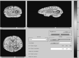
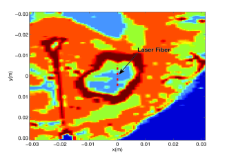
Figure 2: Volumetric Image Reconstruction: a) Position of the tumor in the brain, projected on different planes, b) Segmentation of the tissue over ROI, as viewed over transverse plane (at $36^{th}$ slice in $z$ direction). Four tissue types are shown in different colors: CSF: light blue, grey matter: green, white matter: orange, tumor: red. Dashed red lines shows position of laser fiber.

Fig. 2 illustrates the tissue segmentation in one of the slices within the Region Of Interest (ROI). As Fig. 2 shows, there exist four tissue types within the ROI: Cerebrospinal Fluid (CSF), grey matter, white matter, and tumor tissue. We consider the corresponding optical attenuation for each of these tissues to be uncertain. Hence, we have four uncertain parameters. The optical attenuation coefficient for the CSF, denoted by $\mu_{1}$, is assumed to be uniformly distributed between $10\ \frac{\text{1}}{\text{m}}$ and $300\ \frac{\text{1}}{\text{m}}$, i.e., $\mu_{1}\sim\mathcal{U}[10,300]$, while all the other optical attenuation coefficients are assumed to be uniformly distributed between $10\ \frac{\text{1}}{\text{m}}$ and $400\ \frac{\text{1}}{\text{m}}$, i.e., $\mu_{i}\sim\mathcal{U}[10,400],\ i=2,3,4$. All the other physical properties like conductivity, perfusion, etc, are assumed to be known and are given in Table 2. For the LITT process, we assumed the laser power to be 11.5 watts and heating time period is considered to be $90$ sec.

Table 2: Constitutive Data used in numerical simulations  [38, 58]

$\Lambda$ $\frac{W}{m\cdot K}$	$\omega$ $\frac{kg}{m^{3}s}$	$\rho$ $\frac{kg}{m^{3}}$	$c_{blood}$ $\frac{J}{kg\cdot K}$	$c$ $\frac{J}{kg\cdot K}$
0.527	9.0	1045	3840	3600

To perform the estimation process, we have generated fully sampled synthetic measurement data using a random realization of the optical attenuation coefficient $\mu$. In detail, we used $(\mu_{1},\mu_{2},\mu_{3},\mu_{4})=(111.39,218.75,383.01,385.96)\;\frac{1}{\text{m}}$ to generate the temperature field through the Pennes bioheat model. The obtained temperature field was then used in Eq. (4) to generate the corresponding fully-sampled measurement data. The Signal to Noise Ratio (SNR) is assumed to be 50 in this experiment. Table 3 shows the numerical values of the parameters involved in the sensor structure.

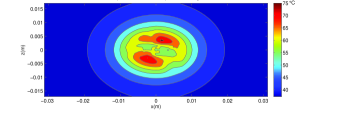
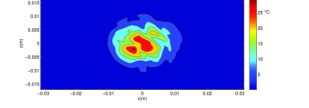
Figure 3: Volumetric Image Reconstruction: a) mean (^∘C) and b) standard deviation of temperature (^∘C) over the ROI crossing through the laser fiber, projected x-z plane.

Table 3: Volumetric Image Reconstruction: parameter values involved in sensor model

Parameter	Value
$\theta$ (rad)	$\pi/3$
$T_{1}$ (sec.)	4.31 (CSF), 1.035 (grey), 0.63 (white), 0.8 (tumor)
$T_{2}^{*}$ (ms)	10 (CSF), 70 (grey), 100 (white), 80 (tumor)
$T_{R}$ (sec.)	0.544
$\Delta\omega_{0}$ (rad)	0
$T_{E}$ (ms)	$25$
$\gamma$ (MHz/T)	42.58
$\alpha$ (ppm/C)	$-0.0102$
$B_{0}$ (T)	$1.5$

A set of 161 Conjugate Unscented Transform (CUT) points [45] (which accurately evaluate upto $8^{th}$ order polynomial integrals) are used to capture the uncertainty in the temperature field due to the presence of uncertain optical attenuation coefficients. Fig. 3 illustrates the mean and standard deviation of the temperature field over an $x-z$ slice co-planar with the laser fiber.

As discussed in Section 5, the variance maximization technique is utilized to approximate $k-$space location with the highest information content for the data acquisition. Fig. 4 illustrates 100 lines in $k-$space with the highest variance. Most of the points lie in center of the $k-$space. The number of points projected on the $k_{x}-k_{y}$ plane is very small comparing to total number of points used in data observation. For instance, in case of using 100 lines on $k-$space for data observation, the proposed technique makes use of only $\frac{100}{128^{2}}\simeq 0.6\%$ of the points on $k_{x}-k_{y}$ plane. Note that this is equivalent with almost 164 times speed up in comparison with full-sampling of $3-$dimensional $k-$space! This can be seen in Fig. 4.

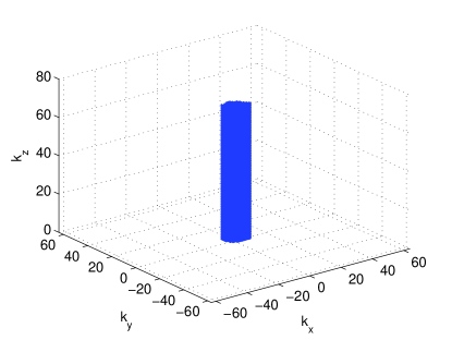
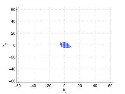
Figure 4: Volumetric Image Reconstruction: Applied points for data observation a) 3-dimensional view b) projection of the points on $k_{x}-k_{y}$ plane. Readout lines are the lines passing through these 100 points.

We performed the model-data fusion using acquired $k-$space samples with the predicted highest variance content. Within the context of the minimum variance framework, Section 6, posterior statistics of optical attenuation coefficients were then found by merging these selected measurements ($k-$space samples) with model predictions. Fig. 5 illustrates the convergence of the posterior estimate of optical attenuation coefficients versus different numbers of measurement data, ranging from 0 to 100 lines. As it is shown in Fig. 5, posterior estimates of parameters, converge to their actual value (denoted by dashed lines) by increasing the number of data observations.

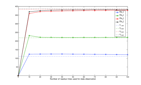
Figure 5: Volumetric Image Reconstruction: Convergence of parameter estimates versus different number of $k-$space readout lines, dashed lines represent the actual value of corresponding attenuation coefficient.

Fig. 6 shows the variance for each of the parameter estimates versus different number of readout lines. As expected, the variance reduces with increasing the number of observations. Note that the associated variance of posterior parameter estimates is much smaller than prior variance of the parameters, i.e. applied model-data fusion have significantly increased our level of confidence about the optical attenuation parameters.

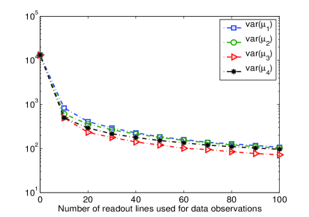
Figure 6: Volumetric Image Reconstruction: Variance of parameter estimates versus different number of $k-$space samples.

Posterior estimates of $\mu$ are then used in the Pennes bioheat equation to estimate the true temperature field. Fig. 7 illustrates temperature field estimate in a representative $x-y$ plane.

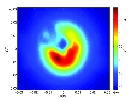
Figure 7: Volumetric Image Reconstruction: Posterior estimate of temperature field (^∘C), using only 100 lines through $k_{z}$, over the $40^{th}$ slice in $z$ direction

Comparison with Other Under-Sampling Schemes

To validate performance of the proposed undersampling technique, we also implemented the approach with two other data acquisition schemes. The first one is rectilinear undersampling, which can be obtained using multi-shot Echo Planar Imaging (EPI) and is widely used in clinical applications. We acquired 100 $k-$space lines, uniformly distributed over $k_{x}-k_{y}$ plane, as shown in Fig. 8. Variable-density Poisson disk undersampling [59] was also used as another scheme for data acquisition. These points are illustrated in Fig. 9. In order to be consistent in our comparisons, we used variable-density Poisson disk sampling and rectilinear approach to generate 100 points over $k_{x}-k_{y}$ plane and then all the points on the lines passing through these points were considered for data acquisition.

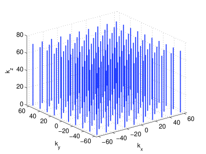
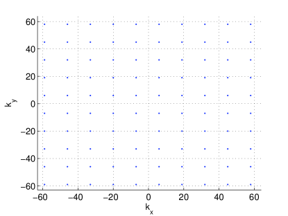
Figure 8: Volumetric Image Reconstruction: Acquired points for data observation (based on rectilinear undersampling) a) 3-dimensional view b) projection of the points on $k_{x}-k_{y}$ plane. Readout lines are the lines passing through these 100 points.

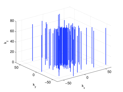
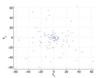
Figure 9: Volumetric Image Reconstruction: Acquired points for data observation (based on variable-density Poisson disk undersampling) a) 3-dimensional view b) projection of the points on $k_{x}-k_{y}$ plane. Readout lines are the lines passing through these 100 points.

Error Analysis

Obtained posterior estimates of $\mu$ from each of these data acquisition techniques are then used in the Pennes bioheat equation to estimate the true temperature field. Fig. 10 represents the error between the true temperature field and its estimate in a representative $x-y$ plane, obtained by different data acquisition schemes. As illustrated in Fig. 10, when the variance maximization is used for data acquisition, the maximum discrepancy between the estimated and true temperature field is less than $4\ ^{\circ}$C, while both other undersampling schemes result in higher value of maximum error.

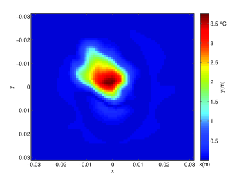
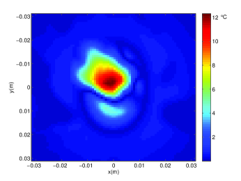
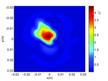
Figure 10: Volumetric Image Reconstruction: The error between posterior estimate and actual temperature field over the $40^{th}$ slice, obtained based on a) Proposed technique, b) Rectilinear undersampling, c) Variable-density Poisson disk undersampling

To further study performance of the proposed technique, we have shown the convergence of the Root Mean Square Error (RMSE) between the temperature estimate and its actual value while using the proposed technique for data acquisition. As shown in Fig. 11, the RMSE in the temperature field estimate consistently reduces with increasing the number of readout lines.

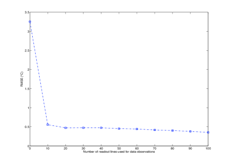
Figure 11: Volumetric Image Reconstruction: RMSE (over all voxels in the full 3D volume) between the estimated and actual temperature fields versus different number of observations (acquired based on the proposed approach).

To summerize, Table 4 represents the maximum and the RMSE between the true temperature field and its estimate, calculated over all voxels in the full 3D volume, when maximum heating occurs. Note that without any observation data the maximum difference between the actual temperature map and its estimate is more than $33\ ^{\circ}$C and by increasing the number of readout lines, it consistently reduces until it reaches to almost $4\ ^{\circ}$C when 100 readout lines (obtained using the proposed data acquisition technique) are used. Also, the RMSE between the temperature estimate and its actual value reduces by a factor of 9. Table 4 also shows the maximum error and RMSE while using rectilinear undersampling and variable-density Poisson disk undersampling. It is clear that variable-density Poisson disk undersampling performs better than rectilinear undersampling, but comparing these values with corresponding error metrics while using variance maximization technique clearly shows performance of the proposed subsampling technique.

Table 4: Volumetric Image Reconstruction: Convergence of error (calculated over all voxels in the full 3D volume) given different numbers of $k-$space samples for model-data fusion. Prior values of error are shown in second column (with zero observations).

Number of readout lines	0	30	50	80	100
maximum error (Proposed Technique) ∘C	33.08	5.16	4.98	4.37	3.81
RMSE (Proposed Technique) ∘C	3.26	0.47	0.45	0.40	0.35
maximum error (Rectilinear Undersampling) ∘C	33.08				12.53
RMSE (Rectilinear Undersampling) ∘C	3.26				1.23
maximum error (Poisson Undersampling) ∘C	33.08				4.52
RMSE (Poisson Undersampling) ∘C	3.26				0.41

8.2 Planar Image Reconstruction

Performance of the proposed subsampling approach is retrospectively validated in fully sampled planar temperature imaging acquired during the thermal ablation process in vivo human brain. The LITT procedure (power = 11.85 watts for a period of 94 sec.) was monitored in real-time using the temperature-sensitive PRF shift technique acquired with a 2D spoiled gradient-echo to generate temperature measurements using GE scanner at every $\Delta t=$5 seconds (TR/FA = 38 ms/30^∘, frequency $\times$ phase = 256 $\times$ 128, FOV = 26 cm², BW = 100 Hz/pixel, slice thickness 5 mm). Fig. 12 shows position of the tumor and the temperature resulting from laser irradiation in the region. Eq. (4) is used to model the MR signal. Numerical values of the parameters involved in sensor structure are shown in Table 5. As shown in Table 5, we assumed $T_{1}$ to be a linear function of tissue temperature [60] in order to incorporate the possible changes in its value due to heating. The value of $T_{1}$ at body temperature, denoted by $T_{1}^{0}$ is considered to be $1.05$ sec.. Also, a normalized MRI image (without any heating involved) is used to incorporate the effect of inhomogeneities in magnetization $M(\mathbf{x})$.

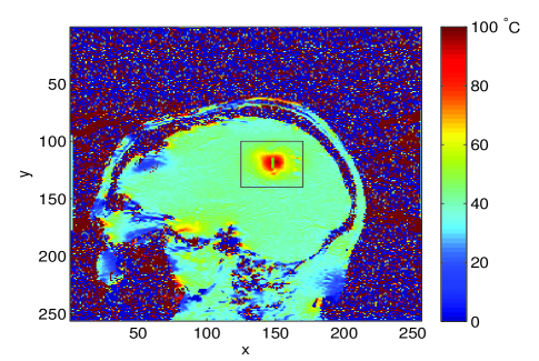
Figure 12: Planar Image Reconstruction: Position of the tumor and the temperature field resulting from MRgLITT (FOV = 26 cm²). Black box and green line inside represent the region of interest and laser fiber, respectively.

Here, we assume that the optical attenuation coefficient $\mu$ is spatially homogeneous and uniformly distributed between $100\ \frac{1}{\text{m}}$ and $400\ \frac{1}{\text{m}}$, i.e. $\mu\sim\mathcal{U}[100,400]$. Note that $\mu$ is the only uncertain parameter while solving the Pennes bioheat equation; all the other parameters are assumed to be known from the physical properties of the tissue, Table 2. A set of 15 Gauss-Legendre quadrature points [61] (which accurately integrate up to the $29^{th}$ order polynomials), spread over the range of uncertain parameter $\mu$, are used to quantify the uncertainty in the temperature field. Fig. 13 illustrates mean and standard deviation of the associated temperature field within the region of interest (ROI).

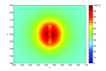
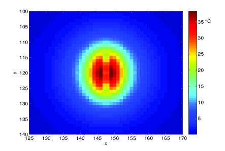
Figure 13: Planar Image Reconstruction: statistics of temperature field over ROI (ROI = 55 mm $\times$ 60 mm), resulted from uncertain $\mu$, a) mean (^∘C), b) standard deviation (^∘C).

Table 5: Planar Image Reconstruction: value of the parameters involved in MRI signal model

Parameter	Value
$\theta$	$\pi/6$ rad
$T2*$	$70$ ms
$T_{E}$	$20$ ms
$\gamma$	42.58 MHz/T
$\alpha$	$-0.0102$ ppm/C
$B_{0}$	$1.5$ T
$T_{1}$	$T_{1}=T_{1}^{0}(1+0.01\Delta u),\quad T_{1}^{0}=1.05$ ms

The proposed technique in Section 5 is utilized to approximate the observation points on $k-$space with largest information content. Given uncertainties in the model, Eq. (1), Fig. 16 shows 20 readout lines that are predicted to have the highest variance in data acquisition. Note that as expected, readout lines pass through the points in center of the $k-$space, i.e. the points with the greatest information content. This corroborates the fact that the points in center of the $k-$space contain more information regarding the main features of the image.

The predicted $k-$space measurements are then retrospectively extracted from the fully sampled data and used in a minimum variance framework to estimate posterior statistics of parameter $\mu$, as described in Section 6. We considered SNR = 25 while using minimum variance framework. Fig. 14 demonstrates convergence behavior for the mean and variance of $\mu$ versus different number of observations. Note that only $\frac{20}{256}\simeq 0.08$ of the total number of readout lines in $k-$space are used for estimation of $\mu$. This results in a speed up factor of 12 (based on division of number of phase lines to the number of readout lines) in comparison with full-sampling of $k-$space, Fig. 16. As a reference, a global optimization to find the value of $\mu$ which results in the least discrepancy between the predicted and fully sampled temperature measurement data was performed. This is shown with a dashed black line in Fig. 14. Results obtained by the proposed approach converges with the result obtained from global optimal and fully sampled technique.

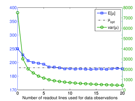
Figure 14: Planar Image Reconstruction: Convergence of $\mu$ estimate versus number of readout lines. Square-blue and circle-green lines represent mean and variance of $\mu$ estimate, respectively. Dashed black line represents the optimal value of $\mu$, obtained from global optimization.

The posterior estimate of $\mu$ is then used in Pennes bioheat equation to estimate the temperature field of the tissue. Fig. 15 illustrates the posterior estimate of the temperature field.

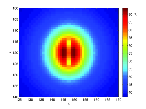
Figure 15: Planar Image Reconstruction: Posterior estimate of the temperature map (ROI = 55 mm $\times$ 60 mm).

Comparison with Other Undersampling Schemes

Similar to previous example, we have also used rectilinear and variable-density Poisson undersampling techniques for $k-$space data acquisition. Fig. 16 and Fig. 16 show 20 readout lines, generated based on rectilinear and variable-density Poisson disk undersampling techniques, respectively.

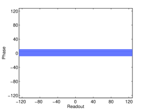
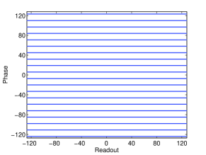
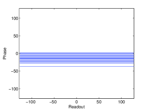
Figure 16: Planar Image Reconstruction: a) The 20 readout lines used for data acquisition, obtained from variance maximization. b) Uniformly distributed readout lines based on rectilinear undersampling. c) Readout lines based on variable-density Poisson disk undersampling.

Given each data acquisition scheme, the predicted $k-$space measurements are used in minimum variance framework to estimate posterior statistics of parameter $\mu$. The obtained posterior estimate of $\mu$ is then used in Pennes bioheat equation to estimate the temperature field of the tissue.

Error Analysis

The error (calculated over ROI) between the posterior estimate of the temperature field and actual temperature map is illustrated in Fig. 17. It is clear from Fig. 17 that the proposed technique results in less error comparing with both rectilinear and variable-density Poisson disk undersampling. Note that when using the proposed method most of error occurs in the edge of ROI due to presence of artifacts, while a considerable amount of error occurs in the center of ROI while using rectilinear or Poisson disk undersampling .

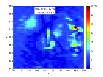
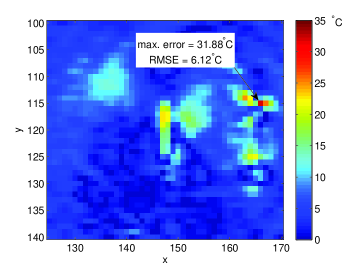
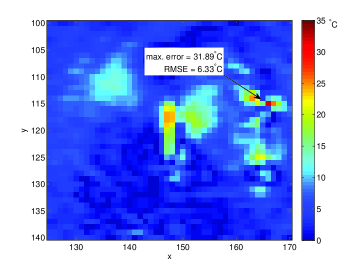
Figure 17: Planar Image Reconstruction: a) The error between the posterior estimate and actual measurement of temperature field, obtained by the proposed technique. Note that the maximum error occurs over the regions close to border. The high value of error in regions near the border of the figure is due to the presence of artifacts in MR temperature data. b) The error between the posterior estimate and actual measurement of temperature field, obtained by using rectilinear undersampling. c) The error between the posterior estimate and actual measurement of temperature field, obtained by using variable-disk Poisson disk undersampling. Note the significant amount of error in center of ROI for cases a and b (ROI = 55 mm $\times$ 60 mm).

To study the effect of the number of data observations on performance of the proposed technique, we have shown the RMSE between the estimated and fully-sampled temperature field in Fig. 18, where in general the value of RMSE reduces with increasing the number of readout lines. Note that a major portion of RMSE is due to presence of artifacts.

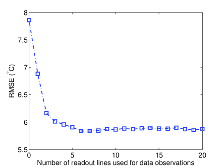
Figure 18: Planar Image Reconstruction: Convergence of RMSE (calculated over ROI) between the acquired temperature map from fully-sampled $k-$space and temperature estimate (obtained from the proposed technique). Note that a major portion of RMSE is due to the presence of artifacts.

8.3 Phantom Experiment

To further validate the proposed approach, we designed a phantom experiment for 3 dimensional temperature imaging. A tissue-mimicking agar phantom ($1.5\%$ gel by weight) was used to simulate the thermal ablation process. The LITT procedure (power = 1 watt for a period of 10 min.) was monitored in real-time using the temperature-sensitive PRF shift technique acquired with EFGRE3D to generate temperature measurements using a GE scanner at every $\Delta t=$15 seconds (TR/FA = 5 ms/5^∘, frequency $\times$ phase = 256 $\times$ 256 $\times$ 26, FOV = 12.8 cm $\times$ 12.8 cm $\times$ 26 mm , BW = 390.62 Hz/pixel, slice thickness 1 mm). Temperature images were recorded over a number of 26 slices in $z-$direction (each with thickness of 1 mm). Fig. 19 shows the position of the laser fiber and corresponding ROI. The parameters used in phantom experiment are shown in Tables 6 and 7. Note that we assumed a linear dependence between $T_{1}$ and temperature in order to incorporate possible changes of $T_{1}$ due to changes in temperature [62]. Also, a normalized MRI image (without any heating involved) was used to account for the effect of inhomogeneities in magnetization $M(\mathbf{x})$.

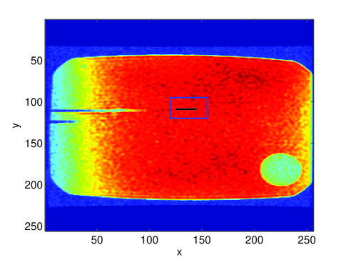
Figure 19: Phantom Experiment: blue rectangle and black line inside represent the ROI and position of laser fiber, respectively.

Table 6: Phantom experiment: Data used in numerical simulations  [63]

$\Lambda$ $\frac{W}{m\cdot K}$	$\omega$ $\frac{kg}{m^{3}s}$	$\rho$ $\frac{kg}{m^{3}}$	$c_{blood}$ $\frac{J}{kg\cdot K}$	$c$ $\frac{J}{kg\cdot K}$
0.6	0	1000	0	3900

Table 7: Phantom experiment: parameter values involved in sensor model

Parameter	Value
$\theta$ (degree)	$5$
$T_{1}$ (sec.)	$2.56+0.1\Delta u$
$T_{2}^{*}$ (ms)	30
$\Delta\omega_{0}$ (rad)	0
$T_{E}$ (ms)	$1.676$
$T_{R}$ (ms)	$5$
$\gamma$ (MHz/T)	42.58
$\alpha$ (ppm/C)	$-0.0102$
$B_{0}$ (T)	$3$
$u_{0}$ (∘C)	$19$

We considered the only uncertain parameter to be the optical attenuation coefficient, which is assumed to be uniformly distributed between 0 and $200$ $\frac{1}{\text{m}}$, i.e. $\mu\in\mathcal{U}(0,200)$. We used a set of 11 Gauss-Legendre quadrature points [61] (which accurately integrates up to the $21^{st}$ order polynomials) to quantify the effect of uncertain parameter $\mu$ on the temperature field and $k-$space signal. Then, the proposed technique was utilized to approximate $k-$space locations with highest amount of variance. Fig. 20 illustrates the $k-$space points found by this approach.

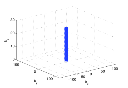
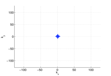
Figure 20: Phantom experiment: Acquired $k-$space points used for data observation (obtained using the proposed technique) a) $3-$dimensional view, b) projected on $k_{x}-k_{y}$ plane.

Obtained $k-$space points are then used in the minimum variance framework to provide posterior statistics of optical attenuation coefficient $\mu$. Similar to previous example, we considered SNR=25 while using minimum variance framework. Fig. 21 represents convergence of mean and variance of $\mu$ estimate versus different number of readout lines. Similar to previous example, we also performed a global optimization to find the value of $\mu$ which results in the least discrepancy between the predicted and fully sampled temperature measurement data (over the ROI). This is shown with a dashed black line in Fig. 21. As one can see, mean estimate of $\mu$ converges to its optimal value by increasing the number of readout lines.

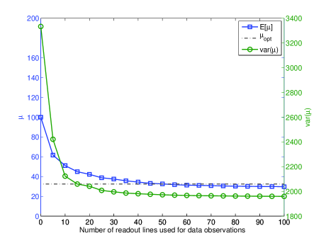
Figure 21: Phantom experiment: Convergence of $\mu$ estimate versus number of observation data. Blue and dashed green lines represent mean and variance of $\mu$ estimate, respectively. Dashed black line represents the optimal value of $\mu$, obtained from global optimization.

The posterior estimate of the temperature map over one of the slices, resulting via using optimally acquired $k-$space points, is shown in Fig. 22.

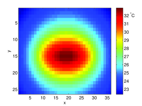
Figure 22: Phantom experiment: Posterior estimate of the temperature map over the $9^{th}$ slice (obtained using the proposed approach for $k-$space subsampling), (ROI = 18 mm $\times$ 13 mm $\times$ 26 mm).

Comparison with Other Undersampling Schemes

We also performed model-data fusion using two other sets of data observations, which are obtained based on rectilinear and variable-density Poisson undersampling techniques. These points are shown in Fig. 23. Note that the same number of points, i.e. 100 readout lines, are used for data acquisition while using both schemes. In rectilinear scheme, lines are homogeneously distributed over $k_{x}-k_{y}$ plane, while most of the lines are concentrated in the center of $k_{x}-k_{y}$ plane in variable-density Poisson disk undersampling.

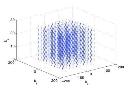
(a) 3-dimensional view

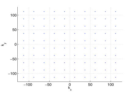
(b) Projection over $k_{x}-k_{y}$ plane

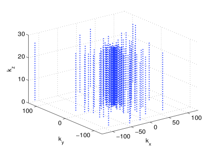
(c) 3-dimensional view

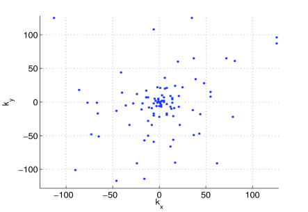
(d) Projection over $k_{x}-k_{y}$ plane

Figure 23: Phantom experiment: Acquired $k-$space points used for data observation a,b) rectilinear scheme, c,d) variable-density Poisson disk undersampling

Error Analysis

Fig. 24 illustrates the discrepancy between posterior temperature estimate and the temperature data acquired from fully sampled $k-$space over one of the slices, while using different data acquisition techniques. As one can see, rectilinear undersampling performs the worst (results in higher value of maximum error) among the applied techniques. Variable-density Poisson disk undersampling performs better than rectilinear scheme, but it results in slightly higher value of maximum error over the $9^{th}$ slice comparing to the proposed approach.

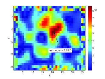
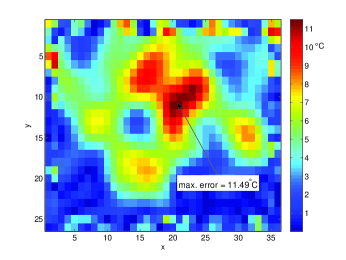
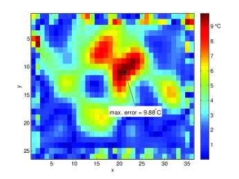
Figure 24: Phantom experiment: The error between the posterior estimate and actual measurement of temperature field over the $9^{th}$ slice, using a) the proposed approach, b) rectilinear undersampling, and c) variable-density Poisson disk undersampling (ROI = 18 mm $\times$ 13 mm $\times$ 26 mm).

Similar to previous examples, we have studied the effect of increasing data observations on performance of the proposed approach. Fig. 25 represents the RMSE between the posterior temperature estimate and acquired temperature data from fully sampled $k-$space versus different numbers of readout lines used for data acquisition. As expected, RMSE reduces by increasing the number of readout lines.

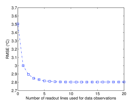
Figure 25: Phantom experiment: Convergence of RMSE (over all voxels inside the ROI) between the acquired temperature map (from fully-sampled $k-$space) and temperature estimate (obtained from the proposed technique).

Finally, Table 8 represents the RMSE (over all voxels inside the ROI) between temperature estimates and acquired temperature data, given different number of readout lines and different data acquisition schemes. Note that there is no change in RMSE value while using rectilinear undersampling. This is expected given that none of the acquired $k-$space points using rectilinear undersampling covers regions with high information content (high information region is mainly concentrated in the center of $k-$space). Hence, almost no information is obtained by performing the model-data fusion. Also as it can be seen in Table 8, proposed technique results in similar value of RMSE comparing with variable-density Poisson disk undersampling method.

Table 8: Phantom experiment: Convergence of error (over all the voxels inside the ROI) given different numbers of $k-$space samples for model-data fusion. Prior values of error are shown in second column (with zero observations).

Number of readout lines	0	5	10	30	50	75	100
RMSE (Proposed Technique)	3.50	3.00	2.89	2.81	2.80	2.80	2.80
RMSE (Rectilinear Undersampling)	3.50						3.50 (using 100 readout lines)
RMSE (variable-density Poisson disk Undersampling)	3.50						2.96 (using 100 readout lines)

9 Discussion

The novelty of the proposed approach demonstrates that locations of high-information content with respect to a model based reconstruction of MR thermometry may be quantitatively identified. The information locations identified are a consequence of the physics based modeling of the laser induced heating and an intelligent characterization of the measurement uncertainties of the acquisition system. Our mathematical model of the MR thermometry acquisition is refined using this set of judiciously selected data observations to reconstruct the thermal image. Intuitively, the accuracy and confidence of the thermal image reconstruction depends on multiple factors like accuracy, information content, and the number of data observations. However, in each example, the presented approach creates an accurate assessment of temperature data while using only subset of the full $k-$space data acquisition. As seen in Fig. 6, Fig. 14, and Fig. 21, the measurement locations chosen sufficiently reduce the posterior variance of model parameters needed to create an accurate thermal image reconstruction.

Generally, accurate temperature image reconstructions are observed in the subsampled examples, Fig. 10, Fig. 17, and Fig. 24. Within the context of the model-data fusion, the accuracy of the Pennes bioheat equation based temperature estimations is improved by the measurement locations identified by our technique. Quantiatively, the posterior value of RMSE is less than its prior value. The majority of errors in the reconstruction may be attributed to artifacts that are not represented in the composite sensor model. Errors are primarily expected in neighborhood regions of the laser fiber.

Currently, MR thermometry is acquired primarily through quantitative phase-sensitive techniques based on the Proton Resonance Frequency (PRF) shift. Compared with current PRF techniques, the benefit of the proposed model-based approach is that the predicted locations of high-information content represent a fraction of the fully sampled $k-$space observations. This implies that an accurate thermal image may be reconstructed in shorter time. Further, the typical PRF approach is susceptible to errors from inter-/intra-scan motion, intravoxel lipid contamination, low SNR, tissue susceptibility changes, magnetic field drift, excessive heating, and modality$-$dependent applicator induced artifacts [64, 65, 66, 67]. The potential data corruption and resulting information loss undermines the confidence and quality in the treatment guidance decisions provided by the MR thermometry. The presented model-based approach provides a rigorous framework to include a model for each source of data corruption artifact. Improved temperature estimate accuracy in the presence of the various sources of image contamination will facilitate a safer, more conformal laser treatment achieved in a variety of circumstances where critical structures may have limited its use.

Mutual information provides the ideal measure to identify $k-$space locations that provide the greatest possible reduction in the model parameter uncertainty. Also, incorporating $k-$space readout trajectories will provide the most physically meaningful models with respect to the underlying MR physics. However, given non-linearities in our physics model, this is computationally prohibitive. In general, maximizing the mutual information between $n$ locations over $k-$space and our thermal image model (with $m$ unknown parameters) would result in $m+n$ dimensional integrals to evaluate the mutual information, which can be computationally expensive due to often large values of $n$. Here, we pursued a computationally tractable approximation and utilized the concept of entropy maximization for approximating optimal $k-$space readout lines. Maximization of the mutual information with respect to a readout trajectory in $k-$space, is a natural progression of these efforts and is the subject of on-going work.

We emphasize that the technique presented in this manuscript is a general methodology which can be utilized with all MR compatible thermal delivery modalities. Algorithm development for MRgLITT is used in this manuscript as a vehicle to focus modeling efforts and is directly extendable to heating induced by High Intensity Focus Ultrasound (HIFU). Highly efficient $k$-space sampling strategies for HIFU may be identified using various models of the ultrasound based heating to allow reconstruction of high quality MR thermometry images with significantly less data compared with fully sampled approaches.

10 Conclusion

In summary, we have presented a model-based information theoretic approach to improve the efficiency of MR thermometry for monitoring MRgLITT procedures. The approach approximates measurement locations in $k-$space with the highest information content with respect to the thermal image reconstruction. The performance of these predicted measurement locations was demonstrated retrospectively in vivo and in silico imaging and is likely to reduce the number of $k-$space measurements needed to accurately reconstruct the thermal image.

References

- [1] R. J. Stafford, D. Fuentes, A. A. Elliott, J. S. Weinberg, and K. Ahrar, “Laser-induced thermal therapy for tumor ablation,” Critical Reviews™ in Biomedical Engineering, vol. 38, no. 1, 2010.
- [2] S. J. Fahrenholtz, R. J. Stafford, F. Maier, J. D. Hazle, and D. Fuentes, “Generalised polynomial chaos-based uncertainty quantification for planning mrglitt procedures,” International Journal of Hyperthermia, vol. 29, no. 4, pp. 324–335, 2013.
- [3] A. Carpentier, D. Chauvet, V. Reina, K. Beccaria, D. Leclerq, R. J. McNichols, A. Gowda, P. Cornu, and J.-Y. Delattre, “Mr-guided laser-induced thermal therapy (litt) for recurrent glioblastomas,” Lasers in surgery and medicine, vol. 44, no. 5, pp. 361–368, 2012.
- [4] H.-J. Schwarzmaier, F. Eickmeyer, W. von Tempelhoff, V. U. Fiedler, H. Niehoff, S. D. Ulrich, Q. Yang, and F. Ulrich, “Mr-guided laser-induced interstitial thermotherapy of recurrent glioblastoma multiforme: preliminary results in 16 patients,” European journal of radiology, vol. 59, no. 2, pp. 208–215, 2006.
- [5] P. R. Jethwa, J. C. Barrese, A. Gowda, A. Shetty, and S. F. Danish, “Magnetic resonance thermometry-guided laser-induced thermal therapy for intracranial neoplasms: initial experience,” Neurosurgery, vol. 71, pp. ons133–ons145, 2012.
- [6] S. E. Norred and J. A. Johnson, “Magnetic resonance-guided laser induced thermal therapy for glioblastoma multiforme: a review,” BioMed research international, vol. 2014, 2014.
- [7] H. Rhim and G. D. Dodd, “Radiofrequency thermal ablation of liver tumors,” Journal of clinical ultrasound, vol. 27, no. 5, pp. 221–229, 1999.
- [8] J. C. Chen, J. A. Moriarty, J. A. Derbyshire, R. D. Peters, J. Trachtenberg, S. D. Bell, J. Doyle, R. Arrelano, G. A. Wright, R. M. Henkelman et al., “Prostate cancer: Mr imaging and thermometry during microwave thermal ablation-initial experience 1,” Radiology, vol. 214, no. 1, pp. 290–297, 2000.
- [9] Y. Anzai, R. Lufkin, A. DeSalles, D. R. Hamilton, K. Farahani, and K. L. Black, “Preliminary experience with mr-guided thermal ablation of brain tumors.” American journal of neuroradiology, vol. 16, no. 1, pp. 39–48, 1995.
- [10] C. J. Simon and D. E. Dupuy, “Percutaneous minimally invasive therapies in the treatment of bone tumors: thermal ablation.” in Seminars in musculoskeletal radiology, vol. 10, no. 2, 2006, pp. 137–144.
- [11] D. J. Curry, A. Gowda, R. J. McNichols, and A. A. Wilfong, “Mr-guided stereotactic laser ablation of epileptogenic foci in children,” Epilepsy & Behavior, vol. 24, no. 4, pp. 408–414, 2012.
- [12] R. J. McNichols, A. Gowda, M. Kangasniemi, J. A. Bankson, R. E. Price, and J. D. Hazle, “Mr thermometry-based feedback control of laser interstitial thermal therapy at 980 nm,” Lasers in surgery and medicine, vol. 34, no. 1, pp. 48–55, 2004.
- [13] S. Roujol, B. D. De Senneville, S. Hey, C. Moonen, and M. Ries, “Robust adaptive extended kalman filtering for real time mr-thermometry guided hifu interventions,” Medical Imaging, IEEE Transactions on, vol. 31, no. 3, pp. 533–542, 2012.
- [14] B. D. De Senneville, S. Roujol, S. Hey, C. Moonen, and M. Ries, “Extended kalman filtering for continuous volumetric mr-temperature imaging,” Medical Imaging, IEEE Transactions on, vol. 32, no. 4, pp. 711–718, 2013.
- [15] D. Fuentes, J. Yung, J. D. Hazle, J. S. Weinberg, and R. J. Stafford, “Kalman filtered mr temperature imaging for laser induced thermal therapies,” Medical Imaging, IEEE Transactions on, vol. 31, no. 4, pp. 984–994, 2012.
- [16] R. E. Kalman, “A new approach to linear filtering and prediction problems,” Journal of Fluids Engineering, vol. 82, no. 1, pp. 35–45, 1960.
- [17] J. Hennig, “K-space sampling strategies,” European radiology, vol. 9, no. 6, pp. 1020–1031, 1999.
- [18] W. A. Willinek, J. Gieseke, R. Conrad, H. Strunk, R. Hoogeveen, M. von Falkenhausen, E. Keller, H. Urbach, C. K. Kuhl, and H. H. Schild, “Randomly segmented central k-space ordering in high-spatial-resolution contrast-enhanced mr angiography of the supraaortic arteries: Initial experience 1,” Radiology, vol. 225, no. 2, pp. 583–588, 2002.
- [19] M. Lustig, D. Donoho, and J. M. Pauly, “Sparse mri: The application of compressed sensing for rapid mr imaging,” Magnetic resonance in medicine, vol. 58, no. 6, pp. 1182–1195, 2007.
- [20] A. Majumdar, R. K. Ward, and T. Aboulnasr, “Compressed sensing based real-time dynamic mri reconstruction,” Medical Imaging, IEEE Transactions on, vol. 31, no. 12, pp. 2253–2266, 2012.
- [21] N. Todd, G. Adluru, A. Payne, E. V. DiBella, and D. Parker, “Temporally constrained reconstruction applied to mri temperature data,” Magnetic Resonance in Medicine, vol. 62, no. 2, pp. 406–419, 2009.
- [22] R. Chartrand, “Fast algorithms for nonconvex compressive sensing: Mri reconstruction from very few data,” in Biomedical Imaging: From Nano to Macro, 2009. ISBI’09. IEEE International Symposium on. IEEE, 2009, pp. 262–265.
- [23] N. Todd, A. Payne, and D. L. Parker, “Model predictive filtering for improved temporal resolution in mri temperature imaging,” Magnetic Resonance in Medicine, vol. 63, no. 5, pp. 1269–1279, 2010.
- [24] P. Gaur and W. A. Grissom, “Accelerated mri thermometry by direct estimation of temperature from undersampled k-space data,” Magnetic Resonance in Medicine, 2014.
- [25] N. Todd, U. Vyas, J. de Bever, A. Payne, and D. L. Parker, “Reconstruction of fully three-dimensional high spatial and temporal resolution mr temperature maps for retrospective applications,” Magnetic Resonance in Medicine, vol. 67, no. 3, pp. 724–730, 2012.
- [26] H. Odéen, N. Todd, M. Diakite, E. Minalga, A. Payne, and D. L. Parker, “Sampling strategies for subsampled segmented epi prf thermometry in mr guided high intensity focused ultrasound,” Medical physics, vol. 41, no. 9, p. 092301, 2014.
- [27] T. Song, A. F. Laine, Q. Chen, H. Rusinek, L. Bokacheva, R. P. Lim, G. Laub, R. Kroeker, and V. S. Lee, “Optimal k-space sampling for dynamic contrast-enhanced mri with an application to mr renography,” Magnetic Resonance in Medicine, vol. 61, no. 5, pp. 1242–1248, 2009.
- [28] F. Vogt, H. Eggebrecht, G. Laub, R. Kroeker, M. Schmidt, J. Barkhausen, and S. Ladd, “High spatial and temporal resolution mra (twist) in acute aortic dissection,” in Proceedings of the 15th Annual Meeting of ISMRM, Berlin, Germany, 2007, p. 92.
- [29] R. Lim, M. Shapiro, E. Wang, M. Law, J. Babb, L. Rueff, J. Jacob, S. Kim, R. Carson, T. Mulholland et al., “3d time-resolved mr angiography (mra) of the carotid arteries with time-resolved imaging with stochastic trajectories: comparison with 3d contrast-enhanced bolus-chase mra and 3d time-of-flight mra,” American Journal of Neuroradiology, vol. 29, no. 10, pp. 1847–1854, 2008.
- [30] E. J. Candès and M. B. Wakin, “An introduction to compressive sampling,” Signal Processing Magazine, IEEE, vol. 25, no. 2, pp. 21–30, 2008.
- [31] S. Vasanawala, M. Murphy, M. T. Alley, P. Lai, K. Keutzer, J. M. Pauly, and M. Lustig, “Practical parallel imaging compressed sensing mri: Summary of two years of experience in accelerating body mri of pediatric patients,” in Biomedical Imaging: From Nano to Macro, 2011 IEEE International Symposium on. IEEE, 2011, pp. 1039–1043.
- [32] G. Marseille, R. De Beer, M. Fuderer, A. Mehlkopf, and D. van Ormondt, “Bayesian estimation of mr images from incomplete raw data,” in Maximum Entropy and Bayesian Methods. Springer, 1996, pp. 13–22.
- [33] O. Brihuega-Moreno, F. P. Heese, and L. D. Hall, “Optimization of diffusion measurements using cramer-rao lower bound theory and its application to articular cartilage,” Magnetic resonance in medicine, vol. 50, no. 5, pp. 1069–1076, 2003.
- [34] D. H. Poot, A. J. den Dekker, E. Achten, M. Verhoye, and J. Sijbers, “Optimal experimental design for diffusion kurtosis imaging,” Medical Imaging, IEEE Transactions on, vol. 29, no. 3, pp. 819–829, 2010.
- [35] M. Cercignani and D. C. Alexander, “Optimal acquisition schemes for in vivo quantitative magnetization transfer mri,” Magnetic resonance in medicine, vol. 56, no. 4, pp. 803–810, 2006.
- [36] T. M. Cover and J. A. Thomas, Elements of information theory. John Wiley & Sons, 2012.
- [37] H. H. Pennes, “Analysis of tissue and arterial blood temperatures in the resting human forearm,” Journal of applied physiology, vol. 85, no. 1, pp. 5–34, 1948.
- [38] A. J. Welch, “The thermal response of laser irradiated tissue,” Quantum Electronics, IEEE Journal of, vol. 20, no. 12, pp. 1471–1481, 1984.
- [39] J. Hindman, “Proton resonance shift of water in the gas and liquid states,” The Journal of Chemical Physics, vol. 44, no. 12, pp. 4582–4592, 1966.
- [40] R. Madankan, P. Singla, T. Singh, and P. D. Scott, “Polynomial-chaos-based bayesian approach for state and parameter estimations,” Journal of Guidance, Control, and Dynamics, vol. 36, no. 4, pp. 1058–1074, 2013.
- [41] R. Madankan, S. Pouget, P. Singla, M. Bursik, J. Dehn, M. Jones, A. Patra, M. Pavolonis, E. Pitman, T. Singh et al., “Computation of probabilistic hazard maps and source parameter estimation for volcanic ash transport and dispersion,” Journal of Computational Physics, vol. 271, pp. 39–59, 2014.
- [42] D. Xiu and G. E. Karniadakis, “The wiener–askey polynomial chaos for stochastic differential equations,” SIAM Journal on Scientific Computing, vol. 24, no. 2, pp. 619–644, 2002.
- [43] N. Wiener, “The homogeneous chaos,” American Journal of Mathematics, pp. 897–936, 1938.
- [44] A. H. Jazwinski, Stochastic Processes and Filtering Theory, R. Bellman, Ed. Academic Press, 1970.
- [45] A. Nagavenkat, P. Singla, and T. Singh, “The conjugate unscented transform-an approach to evaluate multi-dimensional expectation integrals.” Proceedings of the American Control Conference, June 2012.
- [46] F. Bourgault, A. A. Makarenko, S. B. Williams, B. Grocholsky, and H. F. Durrant-Whyte, “Information based adaptive robotic exploration,” in Intelligent Robots and Systems, 2002. IEEE/RSJ International Conference on, vol. 1. IEEE, 2002, pp. 540–545.
- [47] S. MartíNez and F. Bullo, “Optimal sensor placement and motion coordination for target tracking,” Automatica, vol. 42, no. 4, pp. 661–668, 2006.
- [48] R. Tharmarasa, T. Kirubarajan, and M. L. Hernandez, “Large-scale optimal sensor array management for multitarget tracking,” Systems, Man, and Cybernetics, Part C: Applications and Reviews, IEEE Transactions on, vol. 37, no. 5, pp. 803–814, 2007.
- [49] J. L. Williams, J. W. Fisher, and A. S. Willsky, “Approximate dynamic programming for communication-constrained sensor network management,” Signal Processing, IEEE Transactions on, vol. 55, no. 8, pp. 4300–4311, 2007.
- [50] A. Krause, A. Singh, and C. Guestrin, “Near-optimal sensor placements in gaussian processes: Theory, efficient algorithms and empirical studies,” The Journal of Machine Learning Research, vol. 9, pp. 235–284, 2008.
- [51] H.-L. Choi and J. P. How, “Continuous trajectory planning of mobile sensors for informative forecasting,” Automatica, vol. 46, no. 8, pp. 1266–1275, 2010.
- [52] B. J. Julian, M. Angermann, M. Schwager, and D. Rus, “Distributed robotic sensor networks: An information-theoretic approach,” The International Journal of Robotics Research, vol. 31, no. 10, pp. 1134–1154, 2012.
- [53] R. Madankan, N. Adurthi, P. Singla, and T. Singh, “A dynamic data monitoring approach for source parameter estimation of plume dispersion phenomenon,” Atmospheric Environment, vol. submitted.
- [54] R. Madankan, P. Singla, and T. Singh, “Parameter estimation of atmospheric release incidents using maximal information collection,” Dynamic Data-Driven Environmental Systems Science, 5-7 Novamber 2014.
- [55] S. Yan, L. Nie, C. Wu, and Y. Guo, “Linear dynamic sparse modelling for functional mr imaging,” Brain Informatics, vol. 1, no. 1-4, pp. 11–18, 2014.
- [56] A. Gelb, Applied Optimal Estimation. MIT Press, 1974.
- [57] B. B. Avants, N. J. Tustison, G. Song, P. A. Cook, A. Klein, and J. C. Gee, “A reproducible evaluation of ants similarity metric performance in brain image registration,” Neuroimage, vol. 54, no. 3, pp. 2033–2044, 2011.
- [58] F. Duck, “Physical properties of tissue: a comprehensive reference book. 1990,” London, UK: Academic.
- [59] S. A. Mitchell, A. Rand, M. S. Ebeida, and C. Bajaj, “Variable radii poisson-disk sampling, extended version,” in Proceedings of the 24th Canadian Conference on Computational Geometry, vol. 5, 2012.
- [60] V. Rieke and K. Butts Pauly, “Mr thermometry,” Journal of Magnetic Resonance Imaging, vol. 27, no. 2, pp. 376–390, 2008.
- [61] F. B. Hildebrand, Introduction to numerical analysis. Courier Corporation, 1987.
- [62] P. T. Vesanen, K. C. Zevenhoven, J. O. Nieminen, J. Dabek, L. T. Parkkonen, and R. J. Ilmoniemi, “Temperature dependence of relaxation times and temperature mapping in ultra-low-field mri,” Journal of Magnetic Resonance, vol. 235, pp. 50–57, 2013.
- [63] B. A. Taylor, K.-P. Hwang, A. M. Elliott, A. Shetty, J. D. Hazle, and R. J. Stafford, “Dynamic chemical shift imaging for image-guided thermal therapy: analysis of feasibility and potential,” Medical physics, vol. 35, no. 2, pp. 793–803, 2008.
- [64] J. D. Poorter, “Noninvasive mri thermometry with the proton resonance frequency method: study of susceptibility effects,” Magnetic resonance in medicine, vol. 34, no. 3, pp. 359–367, 1995.
- [65] J. Depoorter, C. Dewagter, Y. Dedeene, C. Thomsen, F. Stahlberg, and E. Achten, “The proton-resonance-frequency-shift method compared with molecular diffusion for quantitative measurement of two-dimensional time-dependent temperature distribution in a phantom,” Journal of Magnetic Resonance, Series B, vol. 103, no. 3, pp. 234–241, 1994.
- [66] K. Kuroda, K. Oshio, A. H. Chung, K. Hynynen, and F. A. Jolesz, “Temperature mapping using the water proton chemical shift: a chemical shift selective phase mapping method,” Magnetic resonance in medicine, vol. 38, no. 5, pp. 845–851, 1997.
- [67] J. A. de Zwart, F. C. Vimeux, C. Delalande, P. Canioni, and C. T. Moonen, “Fast lipid-suppressed mr temperature mapping with echo-shifted gradient-echo imaging and spectral-spatial excitation,” Magnetic resonance in medicine, vol. 42, no. 1, pp. 53–59, 1999.