Mixed Robust/Average Submodular Partitioning: Fast Algorithms, Guarantees, and Applications to Parallel Machine Learning and Multi-Label Image Segmentation

Abstract

We study two mixed robust/average-case submodular partitioning problems that we collectively call Submodular Partitioning. These problems generalize both purely robust instances of the problem (namely max-min submodular fair allocation (SFA) Golovin (2005) and min-max submodular load balancing (SLB) Svitkina and Fleischer (2008)) and also generalize average-case instances (that is the submodular welfare problem (SWP) Vondrák (2008) and submodular multiway partition (SMP) Chekuri and Ene (2011a)). While the robust versions have been studied in the theory community Goemans et al. (2009); Golovin (2005); Khot and Ponnuswami (2007); Svitkina and Fleischer (2008); Vondrák (2008), existing work has focused on tight approximation guarantees, and the resultant algorithms are not, in general, scalable to very large real-world applications. This is in contrast to the average case, where most of the algorithms are scalable. In the present paper, we bridge this gap, by proposing several new algorithms (including those based on greedy, majorization-minimization, minorization-maximization, and relaxation algorithms) that not only scale to large sizes but that also achieve theoretical approximation guarantees close to the state-of-the-art, and in some cases achieve new tight bounds. We also provide new scalable algorithms that apply to additive combinations of the robust and average-case extreme objectives. We show that these problems have many applications in machine learning (ML). This includes: 1) data partitioning and load balancing for distributed machine algorithms on parallel machines; 2) data clustering; and 3) multi-label image segmentation with (only) Boolean submodular functions via pixel partitioning. We empirically demonstrate the efficacy of our algorithms on real-world problems involving data partitioning for distributed optimization of standard machine learning objectives (including both convex and deep neural network objectives), and also on purely unsupervised (i.e., no supervised or semi-supervised learning, and no interactive segmentation) image segmentation.

Keywords: Submodular optimization, submodular partitioning, data partitioning, parallel computing, greedy algorithm, multi-label image segmentation, data science

1 Introduction

The problem of set partitioning arises in many machine learning (ML) and data science applications. Given a set $V$ of items, an $m$-partition $\pi=(A_{1}^{\pi},A_{2}^{\pi},\dots,A_{m}^{\pi})$ is a size $m$ set of subsets of $V$ (called blocks) that are non-intersecting (i.e., $A_{i}^{\pi}\cap A_{j}^{\pi}=\emptyset$ for all $i\neq j$) and covering (i.e., $\bigcup_{i=1}^{m}A_{i}^{\pi}=V$). The goal of a partitioning algorithm is to produce a partitioning that is measurably good in some way, often based on an aggregation of the judgements of the internal goodness of the resulting blocks.

In data science and machine learning applications, a partitioning is almost always the end result of a clustering (although in some cases a clustering might allow for intersecting subsets) in which $V$ is partitioned into $m$ clusters (which we, in this paper, refer to as blocks). Most clustering problems are based on optimizing an objective that is either a sum, or an average-case, utility where the goal is to optimize the sum of individual cluster costs — this includes the ubiquitous $k$-means procedure Lloyd (1982); Arthur and Vassilvitskii (2007) where the goal is to construct a partitioning based on choosing a set of cluster centers that minimizes the total sum of squared distances between each point and its closest center. More rarely, clustering algorithms may be based on robust objective functions García-Escudero et al. (2010), where the goal is to optimize the worst-case internal cluster cost (i.e., quality of the clustering is based solely on the quality of the worst internal cluster cost within the clustering). The average case vs. worst case cluster cost assessment distinction are extremes along a continuum, although all existing algorithms operate only at, rather than in between, these extremes.

There is another way of categorizing clustering algorithms, and that based on the goal of each resultant cluster. Most of the time, clustering algorithms attempt to produce clusters containing items similar to or near each other (e.g., with $k$-means, a cluster consists of a centroid and a set of nearby points), and dissimilarity exists, ideally, only between different clusters. An alternate possible goal of clustering is to have each block contains as diverse a set of items as possible, where similarity exist between rather than within clusters. For example, partitioning the vertices of a graph into a set of $k$ independent (or, equivalently, stable) sets would fall into this later category, assuming the graph has edges only between similar vertices. This subsumes graph $k$-colorability problems, one of the most well-known of the NP-complete problems, although in some special cases it is solvable in polynomial time Brandstädt (1996); Feder et al. (1999); Hell et al. (2004). This general idea, where the clusters are as internally diverse as possible using some given measure of diversity, has been called anticlustering Valev (1983, 1998); Späth (1986) in the past and, as can be seen from the above, comprises in general some difficult computational problems.

A third way of further delineating cluster problems is based on how each cluster’s internal quality is measured. In most clustering procedures, each cluster $A^{\pi}_{i}$ for $i\in\{1,2,\dots,m\}$ is internally judged based on the same function $f$ regardless of which cluster is being evaluated. The overall clustering is then an aggregation of the vector of $m$ scores $f(A^{\pi}_{1}),f(A^{\pi}_{2}),\dots,f(A^{\pi}_{m})$. We call this strategy a homogeneous clustering evaluation since every cluster is internally evaluated using the same underlying function. An alternate strategy to evaluate a clustering uses a different function for each cluster. For example, in assignment problems, there are $m$ individuals each of whom is assigned a cluster, and each individual might not judge the same cluster identically. In such cases, we have $m$ functions $f_{1},f_{2},\dots,f_{m}$ that, respectively, internally evaluate the corresponding cluster, and the overall clustering evaluation is based on an aggregation of the vector of scores $f_{1}(A^{\pi}_{1}),f_{2}(A^{\pi}_{2}),\dots,f_{m}(A^{\pi}_{m})$. We call this a heterogeneous clustering evaluation.

The above three strategies to determine the form of cluster evaluation (i.e., average vs. robust case, internally similar vs. diverse clusters, and homogeneous vs. heterogeneous internal cluster evaluation) combined with the various ways of judging the internal cluster evaluations, and ways to aggregate the scores, leads to a plethora of possible clustering objectives. Even in the simple cases, however (such as $k$-means, or independent sets of graphs), the problems are generally hard and/or difficult to approximate.

This paper studies partitioning problems that span the range within and across the aforementioned three strategies, and all from the perspective of submodular function based internal cluster evaluations. In particular, we study problems of the following form:

$$\text{Problem 1: }\qquad\max_{\pi\in\Pi}\Bigl{[}(1-\lambda)\min_{i}f_{i}(A_{i}^{\pi})+\frac{\lambda}{m}\sum_{j=1}^{m}f_{j}(A^{\pi}_{j})\Bigr{]},$$ (1)

and

$$\text{Problem 2: }\qquad\min_{\pi\in\Pi}\Bigl{[}(1-\lambda)\max_{i}f_{i}(A^{\pi}_{i})+\frac{\lambda}{m}\sum_{j=1}^{m}f_{j}(A^{\pi}_{j})\Bigr{]},$$ (2)

where $0\leq\lambda\leq 1$, the set of sets $\pi=(A^{\pi}_{1},A^{\pi}_{2},\cdots,A^{\pi}_{m})$ is an ordered partition of a finite set $V$ (i.e, $\cup_{i}A^{\pi}_{i}=V$ and $\forall i\neq j,A^{\pi}_{i}\cap A^{\pi}_{j}=\emptyset$), and $\Pi$ refers to the set of all ordered partitions of $V$ into $m$ blocks. In contrast to the notion of the partition often used in the computer science and mathematical communities, we clarify that an ordered partition $\pi$ is fully characterized by both its constituent blocks $\{A^{\pi}_{i}\}_{i=1}^{m}$ as well as the ordering of the blocks — this allows us to cover assignment problems, where the $i^{\text{th}}$ block is assigned to the $i^{\text{th}}$, potentially distinct, individual. The parameter $\lambda$ controls the objective: $\lambda=1$ corresponds to the average case, $\lambda=0$ to the robust case, and $0<\lambda<1$ is a mixed case. We are unaware, however, of any previous work (other than our own) that allows for a mixing between worst- and average-case objectives in the context of any form of set partitioning. For convenience, we also define $\bar{\lambda}\triangleq 1-\lambda$ in the below. In general, Problems 1 and 2 are hopelessly intractable, even to approximate, but we assume that the $f_{1},f_{2},\cdots,f_{m}$ are all monotone non-decreasing (i.e., $f_{i}(S)\leq f_{i}(T)$ whenever $S\subseteq T$), normalized ($f_{i}(\emptyset)=0$), and submodular Fujishige (2005) (i.e., $\forall S,T\subseteq V$, $f_{i}(S)+f_{i}(T)\geq f_{i}(S\cup T)+f_{i}(S\cap T)$). These assumptions allow us to develop fast, simple, and scalable algorithms that have approximation guarantees, as is done in this paper. These assumptions, moreover, allow us to retain the naturalness and applicability of Problems 1 and 2 to a wide variety of practical problems.

Submodularity is a natural property in many real-world ML applications Wei et al. (2013); Zheng et al. (2014); Nagano et al. (2010); Wei et al. (2014b); Krause et al. (2008a); Jegelka and Bilmes (2011); Das and Kempe (2011); Krause et al. (2008b); Wei et al. (2015). When minimizing, submodularity naturally model notions of interacting costs and complexity, while when maximizing it readily models notions of diversity, summarization quality, and information. Hence, Problem 1 asks for a partition whose blocks each (to the extent that $\lambda$ is close to 0) and that collectively (to the extent that $\lambda$ is close to 1) are diverse, as represented by the submodular functions. The reason for this is that submodular functions are natural at representing diversity, and a subset $A\subseteq V$ is considered diverse, relative to $V$ and considered amongst other sets also of size $|A|$, if $f(A)$ is as large as possible. Problem 2, on the other hand, asks for a partition whose blocks each (to the extent that $\lambda$ is close to 0) and that collectively (to the extent that $\lambda$ is close to 1) are internally similar (as is typical in clustering) or that are redundant, as measured by the set of submodular functions. Taken together, we call Problems 1 and 2 Submodular Partitioning. As described above, we further categorize these problems depending on if the $f_{i}$’s are identical to each other (the homogeneous case) or not (the heterogeneous case). The heterogeneous case clearly generalizes the homogeneous setting, but as we will see, the additional homogeneous structure can be exploited to provide more efficient and/or tighter algorithms.

The paper is organized as follows. We start by motivating Problems 1 and 2 in the context of machine learning, where there are a number of relevant applications, two of which are expounded upon in Sections 1.1 and 1.2, and some of which we ultimately utilize (in Section 4) to evaluate on real-world data. We then provide algorithms for the robust ($\lambda=0$) versions of Problem 1 and Problem 2 in Section 2. Algorithms for Problems 1 and 2 with general $\lambda$ are given in Section 3. We further explore the applications given section 1.1 and 1.2 and provide an empirical validation in Section 4. We conclude in Section 5.

1.1 Data Partitioning for Parallel Machine Learning

Many of today’s statistical learning methods can take advantage of the vast and unprecedented amount of training data that now exists and is readily available, as indeed “there is no data like more data.” On the other hand, big data presents significant computational challenges to machine learning since, while big data is still getting bigger, it is expected that we are nearing the end of Moore’s law Thompson and Parthasarathy (2006), and single threaded computing speed has unfortunately not significantly improved since about 2003. In light of the ever increasing flood of data that is becoming available, it is hence imperative to develop efficient and scalable methods for large scale training of statistical models. One strategy is to develop smarter and more efficient algorithms, and indeed this fervently is being pursued in the machine learning community. Another natural and complementary strategy, also being widely pursued, is via parallel and distributed computing.

Since machine learning procedures are performed over sets of data, one simple way to achieve parallelism is to split the data into chunks each of which resides on a compute node. This is the idea behind many parallel learning approaches such as ADMM Boyd et al. (2011) and distributed neural network training Povey et al. (2014), to name only a few. Such parallel schemes are often performed where the data samples are distributed to their compute nodes in an arbitrary or random fashion. However, there has apparently been very little work on how to intelligently split the data to ensure that the resultant model can be learned in an efficient, or a particularly good, manner.

One way to approach this problem is to consider a class of “utility” functions on the training data. Given a set $V=\{v_{1},\dots,v_{n}\}$ of training data items, suppose that we have a set function $f:2^{V}\to\mathbb{R}_{+}$ that measures the utility of subsets of the data set $V$. That is, given any $A\subseteq V$, $f(A)$ measures the utility of the training data subset $A$ for producing a good resulting trained model. Given a parallel training scheme (e.g., ADMM) with $m$ compute nodes, we consider an $m$-partition $\pi=(A_{1}^{\pi},A_{2}^{\pi},\dots,A_{m}^{\pi})$ of the entire training data $V$, where we send the $i^{\text{th}}$ block $A_{i}^{\pi}$ of the partition $\pi$ to the $i^{\text{th}}$ compute node. If each compute node $i$ has a block of the data $A_{i}^{\pi}$ that is non-representative of the utility of the whole (i.e., $f(A_{i}^{m})\ll f(V)$), the parallel learning algorithm, at each iteration, might result in the compute nodes deducing models that are widely different from each other. Any subsequent aggregation of the models could then result in a joint model that is non-representative of the whole, especially in a non-convex case like deep neural network models. On the other hand, suppose that an intelligent partition $\pi$ of the training data $V$ is achieved such that each block $A_{i}^{\pi}$ is highly representative of the whole (i.e., $f(A_{i}^{m})\approx f(V),\forall i$). In this case, the models deduced at the compute nodes will tend to be close to a model trained on the entire data, and any aggregation of the resulting models (say via ADMM) will likely be better. An intelligent data partition, in fact, may have a positive effect in two ways: 1) it can lead to a better final solution (in the non-convex case), and 2) faster convergence may be achieved even in the convex case thanks to the fact that any “oscillations” between a distributed stage (where the compute nodes are operating on local data) and an aggregation stage (where some form of model average is computed) could be dampened and hence reduced.

It should be noted that the above process should ideally also be done in the context of any necessary parallel load balancing, where data is distributed so that each processing node has roughly the same amount of compute needing to be performed. Our approach above, by contrast, might be instead called “information balancing,”, where we ensure that each node has a representative amount of information so that reasonable consensus solutions are constructed.

In this work, based on the above intuition, we mathematically describe this goal as obtaining an $m$-partition of the data set $V$ such that the worst-case or the average-case utility among all blocks in the partition is maximized. More precisely, this can be formulated Problem 1 above, where the set of sets $\pi=(A^{\pi}_{1},A^{\pi}_{2},\cdots,A^{\pi}_{m})$ forms a partition of the training data $V$. The parameter $\lambda$ controls the nature of the objective. For example, $\lambda=0$ is the robust case, which is particularly important in mission critical applications, such as parallel and distributed computing, where one single poor partition block can significantly slow down an entire parallel machine (as all compute nodes might need to spin block while waiting for a slow node to complete its round of computation). $\lambda=1$ is the average case. Taking a weighted combination of the both robust and average case objectives (the mixed case, $0<\lambda<1$) allows one to balance between optimizing worst-case and overall performance.

A critical aspect of Problem 1 is that submodular functions are an ideal class of functions for modeling information over training data sets. For example, Wei et al. (2015) show that the utility functions of data subsets for training certain machine learning classifiers can be derived as submodular functions. If $f$ is selected as the class of submodular functions that appropriately model the notion of utility for a given machine learning setting (which could be different depending, say, on what form of training one is doing), solving the homogeneous instance of Problem 1 with $f$ as the objective, then, addresses a core goal in modern machine learning on big data sets, namely how to intelligently partition and distribute training data to multiple compute nodes.

It should be noted that a random partition might have a high probability of performing well, and might have exponentially small probability of producing a partition that performs very poorly. This could be used as an argument for utilizing just a random data partitioning procedure. On the other hand, there are also quite likely a small number of partitions that perform exceedingly well and a random partition also has a very small probability of achieving on one of these high quality partitions. Our long-term quest is to develop methods that increase the likelihood that we can discover one of these rare but high performing partitions. Moreover, there are other applications (i.e., locality maximization via bipartite graphs, where the goal is to organize the data so as to improve data locality, as in the work of Li et al. (2015); Alistarh et al. (2015) where a random partition is quite likely to perform very poorly. This again is an additional potential application of our work.

1.2 Multi-label Image Segmentation

Segmenting images into different regions is one of the more important problems in computer vision. Historically, the problem was addressed by finding a MAP solution to to a Markov random field (MRF), where one constructs a distribution $p(y,\bar{x})=\frac{1}{Z}\exp(-E(y,\bar{x}))$. Here, $y=(y_{1},y_{2},\dots,y_{|V|})$ is a set of pixel labels for a set of pixels $V$, $\bar{x}=(\bar{x}_{1},\bar{x}_{2},\dots,\bar{x}_{|V|})$ is a set of pixel values, and where $E(y,\bar{x})$ is an energy function. For binary image segmentation, $y_{i}\in{0,1}$, and for multi-label instance, $y_{i}\in\{0,1,\dots,m-1\}$, and the image labeling problem computes $\max_{y}p(y|\bar{x})$. In many instances Boykov et al. (2001); Boykov and Kolmogorov (2004); Boykov and Veksler (2006), it was found that performing this maximization can be performed by a graph cut algorithm, in particular when the energy function takes the form $E(y,\bar{x})=\sum_{v\in V}\phi_{v}(y_{v},\bar{x}_{v})+\sum_{C\in\mathcal{C}}\phi_{C}(y_{C})$ where $\mathcal{C}$ are the set of cliques of a graph. When the order of the cliques is two, and when the $\phi_{C}$ functions are submodular, the MAP inference problem can be solved via a minimum graph cut algorithm, and if the order if $\phi_{C}$ is larger, then general submodular function minimization Fujishige (2005) (which runs in polynomial time in $|V|$) may be used. This corresponds, however, only to the binary image segmentation problem. In order to perform multi-label image segmentation, there have been various elaborate extensions of the energy functions to support this (e.g., Jegelka and Bilmes (2011); Shelhamer et al. (2014); Heng et al. (2015); Taniai et al. (2015); Kohli et al. (2013); Silberman et al. (2014) to name just a few), but in all cases the energy function $E(y,\bar{x})$ has to be extended to, at the very least, a non-pseudo Boolean function.

Supposing that we know the number of labels $m$ in advance, an alternate strategy for performing multi-label image segmentation that still utilizes a pseudo-Boolean function is to perform a partition of the pixels. Each block of the partition corresponds to one segment, and for a pixel partitioning to make sense in an image segmentation context, it should be the case that each block consists of pixels that are as non-diverse as possible. For example, the pixels consisting of one object (e.g., a car, a tree, a person) tend to have much less diversity than do a set pixels chosen randomly across the image. A natural set partitioning objective to address multi-label image segmentation is then Problem 2, the reason being that submodular functions, when minimized, tend to choose sets that are non-diverse and, when forced also to be large, are redundant. Problem 2 finds a partition that simultaneously minimizes the worst case diversity of any block, and the average case diversity over all blocks. Note that in this case, the energy function $E(y,\bar{x})$ takes on a different form and in order to define it, we need a bit of additional information. The vector $y\in\{0,1,\dots,m-1\}^{V}$ corresponds to the multi-label labeling of all the pixels in the image. For $i\in\{1,2,\dots,m-1\}$ define $A_{i}(y)=\{v\in V:y_{v}=i\}\subseteq V$ be the subset of $V$ corresponding to the pixels with label $i$ in vector $y$. The multi-label energy function then becomes:

$$E(y,\bar{x})=\sum_{v\in V}\phi_{v}(y_{v},\bar{x}_{v})+\Bigl{[}(1-\lambda)\max_{i}f_{i}(A_{i}(y))+\frac{\lambda}{m}\sum_{j=1}^{m}f_{j}(A_{j}(y))\Bigr{]},$$ (3)

and Problem 2 minimizes it. After solving Problem 2 and given the result $\pi$ of such a partition procedure, the pixels corresponding to block $A_{i}^{\pi}$ should, intuitively, correspond to an object. What is interesting about this approach to multi-label segmentation, however, is that the underlying submodular function (or set thereof) is still binary (i.e., it operates on subsets of sets, or equivalently, on vectors Boolean values corresponding to the characteristic vectors of sets). Instead of changing the function being optimized, Problem 2 changes the way that the function is being used to be more appropriate for the multi-label setting. We evaluate Problem 2 for image segmentation in Section 4.

1.3 Sub-categorizations and Related Previous Work

Problem 1:

Special cases of Problem 1 have appeared previously in the literature. Problem 1 with $\lambda=0$ is called submodular fair allocation (SFA), which has been studied mostly in the heterogeneous setting. When $f_{i}$’s are all modular, the tightest algorithm, so far, is to iteratively round an LP solution achieving $O(1/(\sqrt{m}\log^{3}m))$ approximation Asadpour and Saberi (2010), whereas the problem is NP-hard to $1/2+\epsilon$ approximate for any $\epsilon>0$ Golovin (2005). When $f_{i}$’s are submodular, Golovin (2005) gives a matching-based algorithm with a factor $1/(n-m+1)$ approximation that performs poorly when $m\ll n$. Khot and Ponnuswami (2007) propose a binary search algorithm yielding an improved factor of $1/(2m-1)$. Another approach approximates each submodular function by its ellipsoid approximation (non-scalable) and reduces SFA to its modular version leading to an approximation factor of $O(\sqrt{n}m^{1/4}\log n\log^{3/2}m)$. These approaches are theoretically interesting, but they either do not fully exploit the problem structure or cannot scale to large problems. On the other hand, Problem 1 for $\lambda=1$ is called submodular welfare. This problem has been extensively studied in the literature and can be equivalently formulated as submodular maximization under a partition matroid constraint Vondrák (2008). It admits a scalable greedy algorithm that achieves a $1/2$ approximation Fisher et al. (1978). More recently a multi-linear extension based algorithm nicely solves the submodular welfare problem with a factor of $(1-1/e)$ matching the hardness of this problem Vondrák (2008). It is worth noting that the homogeneous instance of the submodular welfare with $m=2$ generalizes the well-known max-cut problem (Goemans and Williamson, 1995), where the submodular objective is defined as the submodular neighborhood function (Iyer and Bilmes, 2013; Schrijver, 2003). Given a set of vertices $X\subset V$, of a graph $G=(V,E)$, the neighborhood function $f(X)$ counts the number of edges that are incident to at least one vertex in $X$, a monotone non-decreasing submodular function. The function $h(X)=f(X)+f(V\setminus X)-f(V)$ is then the cut function, and since the last term is a constant, maximizing $h$ corresponds to the submodular welfare problem. As far as we know, Problem 1 for general $0<\lambda<1$ has not been studied in the literature.

Problem 1 (Max-(Min$+$Avg)) Approximation factor $\lambda=0$, BinSrch Khot and Ponnuswami (2007) $1/(2m-1)$ $\lambda=0$, Matching Golovin (2005) $1/(n-m+1)$ $\lambda=0$, Ellipsoid Goemans et al. (2009) $O(\sqrt{n}m^{1/4}\log n\log^{3/2}m)$ $\lambda=1$, GreedWelfare Fisher et al. (1978) $1/2$ $\lambda=0$, GreedSat^∗ $(1/2-\delta,\frac{\delta}{1/2+\delta})$ $\lambda=0$, MMax^∗ $O(\underset{i}{\min}\frac{1+(|{A}^{\hat{\pi}}_{i}|-1)(1-\kappa_{f_{i}}({A}^{\hat{\pi}}_{i}))}{|A^{\hat{\pi}}_{i}|\sqrt{m}\log^{3}m})$ $\lambda=0$, GreedMax^†∗ $1/m$ $0<\lambda<1$, GeneralGreedSat^∗ $\lambda/2$ $0<\lambda<1$, CombSfaSwp^∗ $\max\{\frac{\beta\alpha}{\bar{\lambda}\beta+\alpha},\lambda\beta\}$ $0<\lambda<1$, CombSfaSwp^†∗ $\max\{\min\{\alpha,\frac{1}{m}\},\frac{\beta\alpha}{\bar{\lambda}\beta+\alpha},\lambda\beta\}$ $\lambda=0$, Hardness $1/2$ Golovin (2005) $\lambda=1$, Hardness $1-1/e$ Vondrák (2008)

Table 1: Summary of our contributions and existing work on Problem 1. See text for details.

Problem 2:

When $\lambda=0$, Problem 2 is studied as submodular load balancing (SLB). When $f_{i}$’s are all modular, SLB is called minimum makespan scheduling. In the homogeneous setting,  Hochbaum and Shmoys (1988) give a PTAS scheme ($(1+\epsilon)$-approximation algorithm which runs in polynomial time for any fixed $\epsilon$), while an LP relaxation algorithm provides a $2$-approximation for the heterogeneous setting Lenstra et al. (1990). When the objectives are submodular, the problem becomes much harder. Even in the homogeneous setting, Svitkina and Fleischer (2008) show that the problem is information theoretically hard to approximate within $o(\sqrt{n/\log n})$. They provide a balanced partitioning algorithm yielding a factor of $\min\{m,n/m\}$ under the homogeneous setting. They also give a sampling-based algorithm achieving $O(\sqrt{n/\log n})$ for the homogeneous setting. However, the sampling-based algorithm is not practical and scalable since it involves solving, in the worst-case, $O(n^{3}\log n)$ instances of submodular function minimization each of which in general currently requires $O(n^{5}\gamma+n^{6})$ computation Orlin (2009), where $\gamma$ is the cost of a function valuation. Similar to Submodular Fair Allocation, Goemans et al. (2009) applies the same ellipsoid approximation techniques leading to a factor of $O(\sqrt{n}\log n)$ Goemans et al. (2009). When $\lambda=1$, Problem 2 becomes the submodular multiway partition (SMP) for which one can obtain a relaxation based $2$-approximation Chekuri and Ene (2011a) in the homogeneous case. In the non-homogeneous case, the guarantee is $O(\log n)$ Chekuri and Ene (2011b). Similarly, Zhao et al. (2004); Narasimhan et al. (2005) propose a greedy splitting $2$-approximation algorithm for the homogeneous setting. To the best of our knowledge, there does not exist any work on Problem 2 with general $0<\lambda<1$.

We illustrate both the special and the general cases of Problem 1 and 2 in Figure 1.

Problem 2 (Min-(Max$+$Avg)) Approximation factor $\lambda=0$, Balanced^† Svitkina and Fleischer (2008) $\min\{m,n/m\}$ $\lambda=0$, Sampling Svitkina and Fleischer (2008) $O(\sqrt{n\log n})$ $\lambda=0$, Ellipsoid Goemans et al. (2009) $O(\sqrt{n}\log n)$ $\lambda=1$, GreedSplit^† Zhao et al. (2004); Narasimhan et al. (2005) $2$ $\lambda=1$, Relax Chekuri and Ene (2011a) $O(\log n$) $\lambda=0$, MMin^∗ $\underset{i}{\max}\frac{2|A_{i}^{\pi^{*}}|}{1+(|A_{i}^{\pi^{*}}|-1)(1-\kappa_{f_{i}}(A_{i}^{\pi^{*}}))}$ $\lambda=0$, Lovász ​Round^∗ $m$ $0<\lambda<1$ GeneralLovász ​Round^∗ $m$ $0<\lambda<1$, CombSlbSmp^∗ $\min\{\frac{m\alpha}{m\bar{\lambda}+\lambda},\beta(m\bar{\lambda}+\lambda)\}$ $0<\lambda<1$, CombSlbSmp^†∗ $\min\{m,\frac{m\alpha}{m\bar{\lambda}+\lambda},\beta(m\bar{\lambda}+\lambda)\}$ $\lambda=0$, Hardness^∗ $m$ $\lambda=1$, Hardness $2-2/m$ Ene et al. (2013)

Table 2: Summary of our contributions and existing work on Problem 2.

1.4 Our Contributions

In contrast to Problems 1 and 2 in the average case (i.e., $\lambda=1$), existing algorithms for the worst case ($\lambda=0$) are not scalable. This paper closes this gap, by proposing three new classes of algorithmic frameworks to solve SFA and SLB: (1) greedy algorithms; (2) semigradient-based algorithms; and (3) a Lovász extension based relaxation algorithm.

For SFA, when $m=2$, we formulate the problem as non-monotone submodular maximization, which can be approximated up to a factor of $1/2$ with $O(n)$ function evaluations Buchbinder et al. (2012). For general $m$, we give a simple and scalable greedy algorithm (GreedMax), and show a factor of $1/m$ in the homogeneous setting, improving the state-of-the-art factor of $1/(2m-1)$ under the heterogeneous setting Khot and Ponnuswami (2007). For the heterogeneous setting, we propose a “saturate” greedy algorithm (GreedSat) that iteratively solves instances of submodular welfare problems. We show GreedSat has a bi-criterion guarantee of $(1/2-\delta,{\delta}/{(1/2+\delta)})$, which ensures at least $\lceil m(1/2-\delta)\rceil$ blocks receive utility at least $\delta/(1/2+\delta)OPT$ for any $0<\delta<1/2$. For SLB, we first generalize the hardness result in Svitkina and Fleischer (2008) and show that it is hard to approximate better than $m$ for any $m=o(\sqrt{n/\log n})$ even in the homogeneous setting. We then give a Lovász extension based relaxation algorithm (Lovász ​Round) yielding a tight factor of $m$ for the heterogeneous setting. As far as we know, this is the first algorithm achieving a factor of $m$ for SLB in this setting. For both SFA and SLB, we also obtain more efficient algorithms with bounded approximation factors, which we call majorization-minimization (MMin) and minorization-maximization (MMax).

Next we show algorithms to handle Problems 1 and 2 with general $0<\lambda<1$. We first give two simple and generic schemes (CombSfaSwp and CombSlbSmp), both of which efficiently combines an algorithm for the worst-case problem (special case with $\lambda=0$), and an algorithm for the average case (special case with $\lambda=1$) to provide a guarantee interpolating between the two bounds. Given the efficient algorithms proposed in this paper for the robust (worst case) problems (with guarantee $\alpha$), and an existing algorithm for the average case (say, with a guarantee $\beta$), we can obtain a combined guarantee in terms of $\alpha,\beta$ and $\lambda$. We then generalize the proposed algorithms for SLB and SFA to give more practical algorithmic frameworks to solve Problems 1 and 2 for general $\lambda$. In particular we generalize GreedSat leading to GeneralGreedSat, whose guarantee smoothly interpolates in terms of $\lambda$ between the bi-criterion factor by GreedSat in the case of $\lambda=0$ and the constant factor of $1/2$ by the greedy algorithm in the case of $\lambda=1$. For Problem 2 we generalize Lovász ​Round to obtain a relaxation algorithm (GeneralLovász ​Round) that achieves an $m$-approximation for general $\lambda$. Motivated by the computational limitation of GeneralLovász ​Round we also give a simple and efficient greedy heuristic called GeneralGreedMin that works for the homogeneous setting of Problem 2.

Lastly we demonstrate a number of applications of submodular partitioning in real-world machine learning problems. In particular, corresponding to Sections 1.1 and 1.2, we show Problem 1 is applicable in distributed training of statistical models. Problem 2 is useful for data clustering, image segmentation, and computational load balancing. In the experiments we empirically evaluate Problem 1 on data partitioning for ADMM and distributed deep neural network training. The efficacy of Problem 2 is tested on an unsupervised image segmentation task.

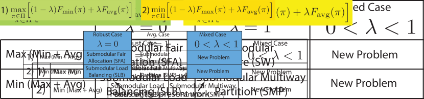
Figure 1: A reminder of the definitions of Problem 1 and 2 (above) and a table that illustrates the cases we focus on in the present work.

2 Robust Submodular Partitioning (Problems 1 and 2 when $\lambda=0$)

Notation: we define $f(j|S)\triangleq f(S\cup j)-f(S)$ as the gain of $j\in V$ in the context of $S\subseteq V$. Then, $f$ is submodular if and only if $f(j|S)\geq f(j|T)$ for all $S\subseteq T$ and $j\notin T$. Also, $f$ is monotone iff $f(j|S)\geq 0,\forall j\notin S,S\subseteq V$. We assume w.l.o.g. that the ground set is $V=\{1,2,\cdots,n\}$.

2.1 Approximation Algorithms for SFA (Problem 1 with $\lambda=0$)

We first investigate a special case of SFA with $m=2$. When $m=2$, the problem becomes

$$\max_{A\subseteq V}g(A),$$ (4)

where $g(A)=\min\{f_{1}(A),f_{2}(V\setminus A)\}$ and is submodular thanks to Theorem 1.

Theorem 1

If $f_{1}$ and $f_{2}$ are monotone submodular, $\min\{f_{1}(A),f_{2}(V\setminus A)\}$ is also submodular.

All proofs for the theoretical results are given in Appendix. Interestingly SFA for $m=2$ can be equivalently formulated as unconstrained submodular maximization. This problem has been well studied in the literature Buchbinder et al. (2012); Dobzinski and Mor (2015); Feige et al. (2011). A simple bi-directional randomized greedy algorithm Buchbinder et al. (2012) solves Eqn 4 with a tight factor of $1/2$. Applying this randomized algorithm to solve SFA then achieves a guarantee of $1/2$ matching the problem’s hardness. However, the same idea does not apply to the general case of $m>2$.

For general $m$, we approach SFA from the perspective of the greedy algorithms. Greedy is often the algorithm that practitioners use for combinatorial optimization problems since they are intuitive, simple to implement, and often lead to very good solutions. In this work we introduce two variants of a greedy algorithm – GreedMax (Alg. 1) and GreedSat (Alg. 2), suited to the homogeneous and heterogeneous settings, respectively.

1:  Input: $f$, $m$, $V$.

2:  Let $A_{1}=,\dots,=A_{m}=\emptyset$; $R=V$.

3:  while $R\neq\emptyset$ do

4:     $j^{*}\in\operatorname*{argmin}_{j}f(A_{j})$;

5:     $a^{*}\in\operatorname*{argmax}_{a\in R}f(a|A_{j^{*}})$

6:     $A_{j^{*}}\leftarrow A_{j^{*}}\cup\{a^{*}\}$; $R\leftarrow R\setminus a^{*}$

7:  end while

8:  Output $\{A_{i}\}_{i=1}^{m}$.

Algorithm 1 GreedMax

GreedMax: The key idea of GreedMax (see Alg. 1) is to greedily add an item with the maximum marginal gain to the block whose current solution is minimum. Initializing $\{A_{i}\}_{i=1}^{m}$ with the empty sets, the greedy flavor also comes from that it incrementally grows the solution by greedily improving the overall objective $\min_{i=1,\dots,m}f_{i}(A_{i})$ until $\{A_{i}\}_{i=1}^{m}$ forms a partition. Besides its simplicity, Theorem 2 offers the optimality guarantee.

Theorem 2

Under the homogeneous setting ($f_{i}=f$ for all $i$), GreedMax is guaranteed to find a partition $\hat{\pi}$ such that

$$\min_{i=1,\dots,m}f(A_{i}^{\hat{\pi}})\geq\frac{1}{m}\max_{\pi\in\Pi}\min_{i=1,\dots,m}f(A_{i}^{\pi}).$$ (5)

By assuming the homogeneity of the $f_{i}$’s, we obtain a very simple $1/m$-approximation algorithm improving upon the state-of-the-art factor $1/(2m-1)$ Khot and Ponnuswami (2007). Thanks to the lazy evaluation trick as described in Minoux (1978), Line 1 in Alg. 1 need not to recompute the marginal gain for every item in each round, leading GreedMax to scale to large data sets.

1:  Input: $\epsilon$, $\{f_{i}\}_{i=1}^{m}$, $m$, $V$, $\alpha$.

2:  Let $\bar{F}^{c}(\pi)=\frac{1}{m}\sum_{i=1}^{m}\min\{f_{i}(A^{\pi}_{i}),c\}$.

3:  Let $c_{\min}=0$, $c_{\max}=\min_{i}f_{i}(V)$

4:  while $c_{\max}-c_{\min}\geq\epsilon$ do

5:     $c=\frac{1}{2}(c_{\max}+c_{\min})$

6:     $\hat{\pi}^{c}\in\operatorname*{argmax}_{\pi\in\Pi}\bar{F}^{c}(\pi)$ // solved by GreedSWP (Alg 3)

7:     if $\bar{F}^{c}(\hat{\pi}^{c})<\alpha c$ then

8:        $c_{\max}=c$

9:     else

10:        $c_{\min}=c$; $\hat{\pi}\leftarrow\hat{\pi}^{c}$

11:     end if

12:  end while

13:  Output: $\hat{\pi}$.

Algorithm 2 GreedSat

  Input: $\{f_{i}\}_{i=1}^{m}$, $c$, $V$

  Initialize: $A_{1}=,\dots,=A_{m}=\emptyset$, and $R\leftarrow V$

while $R\neq\emptyset$ do

       for $i=1,\dots,m$ do

             $\delta_{i}=\max_{r\in R}\min\{f_{i}(A_{i}\cup r),c\}-\min\{f_{i}(A_{i}),c\}$

            $a_{i}\in\operatorname*{argmax}_{r\in R}\min\{f_{i}(A_{i}\cup r),c\}-\min\{f_{i}(A_{i}),c\}$

            

      $j\in\operatorname*{argmax}_{i}\delta(i)$

      

      $A_{j}\leftarrow A_{j}\cup\{a_{j}\}$

      $R\leftarrow R\setminus a_{j}$

      

Output $\hat{\pi}^{c}=(A_{1},\dots,A_{m})$.

Algorithm 3 GreedSWP

GreedSat: Though simple and effective in the homogeneous setting, GreedMax performs arbitrarily poorly under the heterogeneous setting.Consider the following example: $V=\{v_{1},v_{2}\}$, $f_{1}(v_{1})=1,f_{1}(v_{2})=0,f_{1}(\{v_{1},v_{2}\})=1,f_{2}(v_{1})=1+\epsilon,f_{2}(v_{2})=1$, $f_{2}(\{v_{1},v_{2}\})=2+\epsilon$. $f_{1}$ and $f_{2}$ are monotone submodular. The optimal partition is to assign $v_{1}$ to $f_{1}$ and $v_{2}$ to $f_{2}$ leading to a solution of value $1$. However, GreedMax may assign $v_{1}$ to $f_{2}$ and $v_{2}$ to $f_{1}$ leading to a solution of value $0$. Therefore, GreedMax performs arbitrarily poorly on this example.

To this end we provide another algorithm – “Saturate” Greedy (GreedSat, see Alg. 2). The key idea of GreedSat is to relax SFA to a much simpler problem – Submodular Welfare (SWP), i.e., Problem 1 with $\lambda=0$. Similar in flavor to the one proposed in Krause et al. (2008b) GreedSat defines an intermediate objective $\bar{F}^{c}(\pi)=\sum_{i=1}^{m}f_{i}^{c}(A_{i}^{\pi})$, where $f_{i}^{c}(A)=\frac{1}{m}\min\{f_{i}(A),c\}$ (Line 2). The parameter $c$ controls the saturation in each block. It is easy to verify that $f_{i}^{c}$ satisfies submodularity for each $i$. Unlike SFA, the combinatorial optimization problem $\max_{\pi\in\Pi}\bar{F}^{c}(\pi)$ (Line 2) is much easier and is an instance of SWP. In this work, we solve Line 2 using the greedy algorithm as described in Alg 3, which attains a constant 1/2-approximation Fisher et al. (1978). Moreover the lazy evaluation trick also applies for Alg 3 enabling the wrapper algorithm GreedSat scalable to large data sets. One can also use a more computationally expensive multi-linear relaxation algorithm as given in Vondrák (2008) to solve Line 2 with a tight factor $\alpha=(1-1/e)$. Setting the input argument $\alpha$ as the approximation factor for Line 2, the essential idea of GreedSat is to perform a binary search over the parameter $c$ to find the largest $c^{*}$ such that the returned solution $\hat{\pi}^{c^{*}}$ for the instance of SWP satisfies $\bar{F}^{c^{*}}(\hat{\pi}^{c^{*}})\geq\alpha c^{*}$. GreedSat terminates after solving $O(\log(\frac{\min_{i}f_{i}(V)}{\epsilon}))$ instances of SWP. Theorem 3 gives a bi-criterion optimality guarantee.

Theorem 3

Given $\epsilon>0$, $0\leq\alpha\leq 1$ and any $0<\delta<\alpha$, GreedSat finds a partition such that at least $\lceil m(\alpha-\delta)\rceil$ blocks receive utility at least $\frac{\delta}{1-\alpha+\delta}(\max_{\pi\in\Pi}\min_{i}f_{i}(A_{i}^{\pi})-\epsilon)$.

For any $0<\delta<\alpha$ Theorem 3 ensures that the top $\lceil m(\alpha-\delta)\rceil$ valued blocks in the partition returned by GreedSat are $(\delta/(1-\alpha+\delta)-\epsilon)$-optimal. $\delta$ controls the trade-off between the number of top valued blocks to bound and the performance guarantee attained for these blocks. The smaller $\delta$ is, the more top blocks are bounded, but with a weaker guarantee. We set the input argument $\alpha=1/2$ (or $\alpha=1-1/e$) as the worst-case performance guarantee for solving SWP so that the above theoretical analysis follows. However, the worst-case is often achieved only by very contrived submodular functions. For the ones used in practice, the greedy algorithm often leads to near-optimal solution (Krause et al. (2008b) and our own observations). Setting $\alpha$ as the actual performance guarantee for SWP (often very close to 1) can improve the empirical bound, and we, in practice, typically set $\alpha=1$ to good effect.

1:  Input: $\{f_{i}\}_{i=1}^{m}$, $m$, $V$, partition $\pi^{0}$.

2:  Let $t=0$.

3:  repeat

4:     for $i=1,\dots,m$ do

5:        Pick a subgradient $h_{i}$ at $A_{i}^{\pi^{t}}$ for $f_{i}$.

6:     end for

7:     $\pi^{t+1}\in\operatorname*{argmax}_{\pi\in\Pi}\min_{i}h_{i}(A^{\pi}_{i})$

8:     $t=t+1$;

9:  until $\pi^{t}=\pi^{t-1}$

10:  Output: $\hat{\pi}\in\operatorname*{argmax}_{\pi=\pi^{1},\dots,\pi^{t}}\min_{i}f_{i}(A_{i}^{\pi})$.

Algorithm 4 MMax

MMax: In parallel to GreedSat, we also introduce a semi-gradient based approach for solving SFA under the heterogeneous setting. We call this algorithm minorization-maximization (MMax, see Alg. 4). Similar to the ones proposed in Iyer et al. (2013a); Iyer and Bilmes (2013, 2012b), the idea is to iteratively maximize tight lower bounds of the submodular functions. Submodular functions have tight modular lower bounds, which are related to the subdifferential $\partial_{f}(Y)$ of the submodular set function $f$ at a set $Y\subseteq V$, which is defined Fujishige (2005) as:

$$\partial_{f}(Y)=\{y\in\mathbb{R}^{n}:f(X)-y(X)\geq f(Y)-y(Y)\;\text{for all }X\subseteq V\}.$$ (6)

For a vector $x\in\mathbb{R}^{V}$ and $X\subseteq V$, we write $x(X)=\sum_{j\in X}x(j)$. Denote a subgradient at $Y$ by $h_{Y}\in\partial_{f}(Y)$, the extreme points of $\partial_{f}(Y)$ may be computed via a greedy algorithm: Let $\sigma$ be a permutation of $V$ that assigns the elements in $Y$ to the first $|Y|$ positions ($\sigma(i)\in Y$ if and only if $i\leq|Y|$). Each such permutation defines a chain with elements $S_{0}^{\sigma}=\emptyset$, $S^{\sigma}_{i}=\{\sigma(1),\sigma(2),\dots,\sigma(i)\}$, and $S^{\sigma}_{|Y|}=Y$. An extreme point $h^{\sigma}_{Y}$ of $\partial_{f}(Y)$ has each entry as

$$h^{\sigma}_{Y}(\sigma(i))=f(S^{\sigma}_{i})-f(S^{\sigma}_{i-1}).$$ (7)

Defined as above, $h^{\sigma}_{Y}$ forms a lower bound of $f$, tight at $Y$ — i.e., $h^{\sigma}_{Y}(X)=\sum_{j\in X}h^{\sigma}_{Y}(j)\leq f(X),\forall X\subseteq V$ and $h^{\sigma}_{Y}(Y)=f(Y)$. The idea of MMax is to consider a modular lower bound tight at the set corresponding to each block of a partition. In other words, at iteration $t+1$, for each block $i$, we approximate $f_{i}$ with its modular lower bound tight at $A_{i}^{\pi^{t}}$ and solve a modular version of Problem 1 (Line 7), which admits efficient approximation algorithms Asadpour and Saberi (2010). MMax is initialized with a partition $\pi^{0}$, which is obtained by solving Problem 1, where each $f_{i}$ is replaced with a simple modular function $f^{\prime}_{i}(A)=\sum_{a\in A}f_{i}(a)$. The following worst-case bound holds:

Theorem 4

MMax achieves a worst-case guarantee of

$$O(\min_{i}\frac{1+(|{A}^{\hat{\pi}}_{i}|-1)(1-\kappa_{f_{i}}({A}^{\hat{\pi}}_{i}))}{|{A}^{\hat{\pi}}_{i}|\sqrt{m}\log^{3}m}),$$

where $\hat{\pi}=({A^{\hat{\pi}}_{1}},\cdots,A^{\hat{\pi}}_{m})$ is the partition obtained by the algorithm, and

$$\kappa_{f}(A)=1-\min_{v\in V}\frac{f(v|A\setminus v)}{f(v)}\in[0,1]$$

is the curvature of a submodular function $f$ at $A\subseteq V$.

When each submodular function $f_{i}$ is modular, i.e., $\kappa_{f_{i}}(A)=0,\forall A\subseteq V,i$, the approximation guarantee of MMax becomes $O(\frac{1}{\sqrt{m}\log^{3}m})$, which matches the performance of the approximation algorithm for the modular problem. When each $f_{i}$ is fully curved, i.e., $\kappa_{f_{i}}=1$, we still obtain a bounded guarantee of $O(\frac{1}{n\sqrt{m}\log^{3}m})$. Theorem 4 suggests that the performance of MMax improves as the curvature $\kappa_{f_{i}}$ of each objective $f_{i}$ decreases. This is natural since MMax essentially uses the modular lower bounds as the proxy for each objective and optimizes with respect to the proxy functions. Lower the curvature of the objectives, the better the modular lower bounds approximate, hence better performance guarantee.

Since the modular version of SFA is also NP-hard and cannot be exactly solved in polynomial time, we cannot guarantee that successive iterations of MMax improves upon the overall objective. However we still obtain the following Theorem giving a bounded performance gap between the successive iterations.

Theorem 5

Suppose modular version of SFA is solved with an approximation factor $\alpha\leq 1$, we have for each iteration $t$ that

$$\min_{i}f_{i}(A_{i}^{\pi_{t}})\geq\alpha\min_{i}f_{i}(A_{i}^{\pi_{t-1}}).$$ (8)

2.2 Approximation Algorithms for SLB (Problem 2 with $\lambda=0$)

In this section, we investigate the problem of submodular load balancing (SLB). It is a special case of Problem 2 with $\lambda=0$. We first analyze the hardness of SLB. We then show a Lovász extension-based algorithm with a guarantee matching the problem’s hardness. Lastly we describe a more efficient supergradient based algorithm.

Existing hardness for SLB is shown to be $o(\sqrt{n/\log n})$ Svitkina and Fleischer (2008). However it is independent of $m$, and Svitkina and Fleischer (2008) assumes $m=\Theta(\sqrt{n/\log n})$ in their analysis. In most of the applications of SLB, we find that the parameter $m$ is such that $m\ll n$ and can sometimes be treated as a constant w.r.t. $n$. To this end we offer a more general hardness analysis that is dependent directly on $m$.

Theorem 6

For any $\epsilon>0$, SLB cannot be approximated to a factor of $(1-\epsilon)m$ for any $m=o(\sqrt{n/\log n})$ with polynomial number of queries even under the homogeneous setting.

Though the proof technique for Theorem 6 mostly carries over from Svitkina and Fleischer (2008), the result strictly generalizes the analysis in Svitkina and Fleischer (2008). For any choice of $m=o(\sqrt{n/\log n})$ Theorem 6 implies that it is information theoretically hard to approximate SLB better than $m$ even for the homogeneous setting. For the rest of the paper, we assume $m=o(\sqrt{n/\log n})$ for SLB, unless stated otherwise. It is worth pointing out that arbitrary partition $\pi\in\Pi$ already achieves the best approximation factor of $m$ that one can hope for under the homogeneous setting. Denote $\pi^{*}$ as the optimal partitioning for SLB, i.e., $\pi^{*}\in\operatorname*{argmin}_{\pi\in\Pi}\max_{i}f(A_{i}^{\pi})$. This can be verified by considering the following:

$$\max_{i}f(A_{i}^{\pi})\leq f(V)\leq\sum_{i=1}^{m}f(A_{i}^{\pi^{*}})\leq m\max_{i}f(A_{i}^{\pi^{*}}).$$ (9)

It is therefore theoretically interesting to consider only the heterogeneous setting.

1:  Input: $\{f_{i}\}_{i=1}^{m}$, $\{\tilde{f}_{i}\}_{i=1}^{m}$, $m$, $V$.

2:  Solve for $\{x^{*}_{i}\}_{i=1}^{m}$ via convex relaxation.

3:  Rounding: Let $A_{1}=,\dots,=A_{m}=\emptyset$.

4:  for $j=1,\dots,n$ do

5:     $\hat{i}\in\operatorname*{argmax}_{i}x^{*}_{i}(j)$; $A_{\hat{i}}=A_{\hat{i}}\cup j$

6:  end for

7:  Output $\hat{\pi}=\{A_{i}\}_{i=1}^{m}$.

Algorithm 5 Lovász ​Round

Lovász ​Round: Next we propose a tight algorithm – Lovász ​Round (see Alg. 5) for the heterogeneous setting of SLB. The algorithm proceeds as follows: (1) apply the Lovász extension of submodular functions to relax SLB to a convex program, which is exactly solved to a fractional solution (Line 5); (2) map the fractional solution to a partition using the $\theta$-rounding technique as proposed in Iyer et al. (2014) (Line 5 - 6). The Lovász extension, which naturally connects a submodular function $f$ with its convex relaxation $\tilde{f}$, is defined as follows: given any $x\in[0,1]^{n}$, we obtain a permutation $\sigma_{x}$ by ordering its elements in non-increasing order, and thereby a chain of sets $S_{0}^{\sigma_{x}}\subset,\dots,\subset S_{n}^{\sigma_{x}}$ with $S_{j}^{\sigma_{x}}=\{\sigma_{x}(1),\dots,\sigma_{x}(j)\}$ for $j=1,\dots,n$. The Lovász extension $\tilde{f}$ for $f$ is the weighted sum of the ordered entries of $x$:

$$\tilde{f}(x)=\sum_{j=1}^{n}x(\sigma_{x}(j))(f(S_{j}^{\sigma_{x}})-f(S_{j-1}^{\sigma_{x}})).$$ (10)

Given the convexity of the $\tilde{f}_{i}$’s , SLB is relaxed to the following convex program:

$$\min_{x_{1},\dots,x_{m}\in[0,1]^{n}}\max_{i}\tilde{f}_{i}(x_{i}),\mbox{ s.t }\sum_{i=1}^{m}x_{i}(j)\geq 1,\text{ for }j=1,\dots,n$$ (11)

Denoting the optimal solution for Eqn 11 as $\{x_{1}^{*},\dots,x_{m}^{*}\}$, the $\theta$-rounding step simply maps each item $j\in V$ to a block $\hat{i}$ such that $\hat{i}\in\operatorname*{argmax}_{i}x^{*}_{i}(j)$ (ties broken arbitrarily). The bound for Lovász ​Round is as follows:

Theorem 7

Lovász ​Round is guaranteed to find a partition $\hat{\pi}\in\Pi$ such that

$$\max_{i}f_{i}(A_{i}^{\hat{\pi}})\leq m\min_{\pi\in\Pi}\max_{i}f_{i}(A_{i}^{\pi})$$

.

We remark that, to the best of our knowledge, LovászRound is the first algorithm that is tight and that gives an approximation in terms of $m$ for the heterogeneous setting.

1:  Input: $\{f_{i}\}_{i=1}^{m}$, $m$, $V$, partition $\pi^{0}$.

2:  Let $t=0$

3:  repeat

4:     for $i=1,\dots,m$ do

5:        Pick a supergradient $m_{i}$ at $A_{i}^{\pi^{t}}$ for $f_{i}$.

6:     end for

7:     $\pi^{t+1}\in\operatorname*{argmin}_{\pi\in\Pi}\max_{i}m_{i}(A^{\pi}_{i})$

8:     $t=t+1$;

9:  until $\pi^{t}=\pi^{t-1}$

10:  Output: $\pi^{t}$.

Algorithm 6 MMin

MMin: Similar to MMax for SFA, we propose Majorization-Minimization (MMin, see Alg. 6) for SLB. Here, we iteratively choose modular upper bounds, which are defined via superdifferentials $\partial^{f}(Y)$ of a submodular function Jegelka and Bilmes (2011) at $Y$:

$$\partial^{f}(Y)=\{y\in\mathbb{R}^{n}:f(X)-y(X)\leq f(Y)-y(Y);\text{for all }X\subseteq V\}.$$ (12)

Moreover, there are specific supergradients Iyer and Bilmes (2012a); Iyer et al. (2013a) that define the following two modular upper bounds (when referring to either one, we use $m^{f}_{X}$):

$$m^{f}_{X,1}(Y)\triangleq f(X)-\!\!\!\!\sum_{j\in X\backslash Y}f(j|X\backslash j)+\!\!\!\!\sum_{j\in Y\backslash X}f(j|\emptyset)\scalebox{1.3}{,}\;\;\;$$

$$m^{f}_{X,2}(Y)\triangleq f(X)-\!\!\!\sum_{j\in X\backslash Y}f(j|V\backslash j)+\!\!\!\!\sum_{j\in Y\backslash X}f(j|X).$$

Then $m^{f}_{X,1}(Y)\geq f(Y)$ and $m^{f}_{X,2}(Y)\geq f(Y),\forall Y\subseteq V$ and $m^{f}_{X,1}(X)=m^{f}_{X,2}(X)=f(X)$. At iteration $t+1$, for each block $i$, MMin replaces $f_{i}$ with a choice of its modular upper bound $m_{i}$ tight at $A_{i}^{\pi^{t}}$ and solves a modular version of Problem 2 (Line 7), for which there exists an efficient LP relaxation based algorithm Lenstra et al. (1990). Similar to MMax, the initial partition $\pi^{0}$ is obtained by solving Problem 2, where each $f_{i}$ is substituted with $f_{i}^{\prime}(A)=\sum_{a\in A}f_{i}(a)$. The following worst-case bound holds:

Theorem 8

MMin achieves a worst-case guarantee of $(2\max_{i}\frac{|A_{i}^{\pi^{*}}|}{1+(|A_{i}^{\pi^{*}}|-1)(1-\kappa_{f_{i}}(A_{i}^{\pi^{*}}))}),$ where $\pi^{*}=(A_{1}^{\pi^{*}},\cdots,A_{m}^{\pi^{*}})$ denotes the optimal partition.

Similar to MMax, we can show that MMin has bounded performance gaps in successive iterations.

Theorem 9

Suppose the modular version of SLB can be solved with an approximation factor $\alpha\geq 1$, we have for each iteration $t$ that

$$\max_{i}f_{i}(A_{i}^{\pi_{t}})\leq\alpha\max_{i}f_{i}(A_{i}^{\pi_{t-1}}).$$ (13)

3 General Submodular Partitioning (Problems 1 and 2 when $0<\lambda<1$)

In this section we study Problem 1 and Problem 2, in the most general case, i.e., $0<\lambda<1$. We use the proposed algorithms for the special cases of Problems 1 and 2 as the building blocks to design algorithms for the general scenarios $(0<\lambda<1)$. We first propose a simple and generic scheme that provides performance guarantee in terms of $\lambda$ for both problems. We then generalize the proposed GreedSat to obtain a more practically interesting algorithm for Problem 1. For Problem 2 we generalize Lovász Round to obtain a relaxation based algorithm.

Extremal Combination Scheme: First we describe the scheme that works for both problem 1 and 2. It naturally combines an algorithm for solving the worst-case problem ($\lambda=0$) with an algorithm for solving the average case ($\lambda=1$). We use Problem 1 as an example, but the same scheme easily works for Problem 2. Denote AlgWC as the algorithm for the worst-case problem (i.e. SFA), and AlgAC as the algorithm for the average case (i.e., SWP). The scheme is to first obtain a partition $\hat{\pi}_{1}$ by running AlgWC on the instance of Problem 1 with $\lambda=0$ and a second partition $\hat{\pi}_{2}$ by running AlgAC with $\lambda=1$. Then we output one of $\hat{\pi}_{1}$ and $\hat{\pi}_{2}$, with which the higher valuation for Problem 1 is achieved. We call this scheme CombSfaSwp. Suppose AlgWC solves the worst-case problem with a factor $\alpha\leq 1$ and AlgAC for the average case with $\beta\leq 1$. When applied to Problem 2 we refer to this scheme as CombSlbSmp ($\alpha\geq 1$ and $\beta\geq 1$). The following guarantee holds for both schemes:

Theorem 10

For any $\lambda\in(0,1)$ CombSfaSwp solves Problem 1 with a factor $\max\{\frac{\beta\alpha}{\bar{\lambda}\beta+\alpha},\lambda\beta\}$ in the heterogeneous case, and $\max\{\min\{\alpha,\frac{1}{m}\},\frac{\beta\alpha}{\bar{\lambda}\beta+\alpha},\lambda\beta\}$ in the homogeneous case. Similarly, CombSlbSmp solves Problem 2 with a factor $\min\{\frac{m\alpha}{m\bar{\lambda}+\lambda},\beta(m\bar{\lambda}+\lambda)\}$ in the heterogeneous case, and $\min\{m,\frac{m\alpha}{m\bar{\lambda}+\lambda},\beta(m\bar{\lambda}+\lambda)\}$ in the homogeneous case.

1:  Input: $\epsilon$, $\{f_{i}\}_{i=1}^{m}$, $m$, $V$, $\lambda$, $\alpha$.

2:  Let $\bar{F}^{c}_{\lambda}(\pi)=\frac{1}{m}\sum_{i=1}^{m}\min\{\bar{\lambda}f_{i}(A^{\pi}_{i})+\lambda\frac{1}{m}\sum_{j=1}^{m}f_{j}(A_{j}^{\pi}),c\}$.

3:  Let $c_{\min}=0$, $c_{\max}=\sum_{i=1}^{m}f_{i}(V)$

4:  while $c_{\max}-c_{\min}\geq\epsilon$ do

5:     $c=\frac{1}{2}(c_{\max}+c_{\min})$

6:     $\hat{\pi}^{c}\in\operatorname*{argmax}_{\pi\in\Pi}\bar{F}^{c}_{\lambda}(\pi)$ // solved by GreedSwp (Alg. 3)

7:     if $\bar{F}^{c}(\hat{\pi}^{c})<\alpha c$ then

8:        $c_{\max}=c$

9:     else

10:        $c_{\min}=c$; $\hat{\pi}\leftarrow\hat{\pi}^{c}$

11:     end if

12:  end while

13:  Output: $\hat{\pi}$.

Algorithm 7 GeneralGreedSat

GeneralGreedSat: The drawback of CombSfaSwp and CombSlbSmp is that they do not explicitly exploit the trade-off between the average-case and worst-case in terms of $\lambda$. To obtain more practically interesting algorithms, we first give GeneralGreedSat (See Alg. 7) that generalizes GreedSat to solve Problem 1 for general $\lambda$. The key idea of GeneralGreedSat is again to relax Problem 1 to a simpler submodular welfare problem (SWP). Similar to GreedSat we define an intermediate objective:

$$\bar{F}^{c}_{\lambda}(\pi)=\frac{1}{m}\sum_{i=1}^{m}\min\{\bar{\lambda}f_{i}(A^{\pi}_{i})+\lambda\frac{1}{m}\sum_{j=1}^{m}f_{j}(A_{j}^{\pi}),c\}.$$ (14)

It is easy to verify that the combinatorial optimization problem $\max_{\pi\in\Pi}\bar{F}^{c}_{\lambda}(\pi)$ (Line 7) can be formulated as the submodular welfare problem, for which we can solve efficiently with GreedSwp (see Alg. 3). Defining $\alpha$ as the optimality guarantee of the algorithm for solving Line 7 GeneralGreedSat solves Problem 1 with the following bounds:

Theorem 11

Given $\epsilon>0$, $0\leq\alpha\leq 1$, and $0\leq\lambda\leq 1$, GeneralGreedSat finds a partition $\hat{\pi}$ that satisfies the following:

$$\bar{\lambda}\min_{i}f_{i}(A_{i}^{\hat{\pi}})+\lambda\frac{1}{m}\sum_{i=1}^{m}f_{i}(A_{i}^{\hat{\pi}})\geq\lambda\alpha(OPT-\epsilon)$$ (15)

where $OPT=\max_{\pi\in\Pi}\bar{\lambda}\min_{i}f_{i}(A_{i}^{\pi})+\lambda\frac{1}{m}\sum_{i=1}^{m}f_{i}(A_{i}^{\pi})$.

Moreover, let $F_{\lambda,i}(\pi)=\bar{\lambda}f_{i}(A_{i}^{\pi})+\lambda\frac{1}{m}\sum_{j=1}^{m}f_{j}(A_{j}^{\pi})$. Given any $0<\delta<\alpha$, there is a set $I\subseteq\{1,\dots,m\}$ such that $|I|\geq\lceil m(\alpha-\delta)\rceil$ and

$$F_{i,\lambda}(\hat{\pi})\geq\max\{\frac{\delta}{1-\alpha+\delta},\lambda\alpha\}(OPT-\epsilon),\forall i\in I.$$ (16)

Eqn 16 in Theorem 11 reduces to Theorem 3 when $\lambda=0$, i.e., it recovers the bi-criterion guarantee in Theorem 3 for the worst-case scenario ($\lambda=0$). Eqn 15 in Theorem 11 implies that $\alpha$-approximation for the average-case objective can almost be recovered by GeneralGreedSat if $\lambda=1$. Moreover Theorem 11 shows that the guarantee of GeneralGreedSat improves as $\lambda$ increases suggesting that Problem 1 becomes easier as the mixed objective weights more on the average-case objective. We also point out that the approximation guarantee of GeneralGreedSat smoothly interpolates the two extreme cases in terms of $\lambda$.

1:  Input: $\{f_{i}\}_{i=1}^{m}$, $\{\tilde{f}_{i}\}_{i=1}^{m}$, $\lambda$, $m$, $V$.

2:  Solve

$$\min_{x_{1},\dots,x_{m}\in[0,1]^{n}}\max_{i}\bar{\lambda}\tilde{f}_{i}(x_{i})+\lambda\frac{1}{m}\sum_{j=1}^{m}\tilde{f}_{j}(x_{j}),\mbox{ s.t }\sum_{i=1}^{m}x_{i}(j)\geq 1,\text{ for }j=1,\dots,n$$ (17)

for $\{x^{*}_{i}\}_{i=1}^{m}$ via convex relaxation.

3:  Rounding: Let $A_{1}=,\dots,=A_{m}=\emptyset$.

4:  for $j=1,\dots,n$ do

5:     $\hat{i}\in\operatorname*{argmax}_{i}x^{*}_{i}(j)$; $A_{\hat{i}}=A_{\hat{i}}\cup j$

6:  end for

7:  Output $\hat{\pi}=\{A_{i}\}_{i=1}^{m}$.

Algorithm 8 GeneralLovász ​Round

GeneralLovász ​Round: Next we focus on designing practically more interesting algorithms for Problem 2 with general $\lambda$. In particular we generalize Lovász ​Round leading to GeneralLovász ​Round as shown in Alg. 8. Sharing the same idea with Lovász ​Round, GeneralLovász ​Round first relaxes Problem 2 as a convex program (defined in Eqn 17) using the Lovász extension of each submodular objective. Given the fractional solution to the convex program $\{x_{i}^{*}\}_{i=1}^{m}$, the algorithm then rounds it to a partition using the $\theta$-rounding technique (Line 8- 6). Note the rounding technique used for GeneralLovász ​Round is the same as in Lovász ​Round. The following Theorem holds:

Theorem 12

GeneralLovász ​Round is guaranteed to find a partition $\hat{\pi}\in\Pi$ such that

$$\max_{i}\bar{\lambda}f_{i}(A_{i}^{\hat{\pi}})+\lambda\frac{1}{m}\sum_{j=1}^{m}f_{j}(A_{j}^{\hat{\pi}})\leq m\min_{\pi\in\Pi}\max_{i}\bar{\lambda}f_{i}(A_{i}^{{\pi}})+\lambda\frac{1}{m}\sum_{j=1}^{m}f_{j}(A_{j}^{{\pi}}).$$ (18)

Theorem 12 generalizes Theorem 7 when $\lambda=0$. Moreover we achieve a factor of $m$ by GeneralLovász Round for any $\lambda$. Though the approximation guarantee is independent of $\lambda$ the algorithm naturally exploits the trade-off between the worst-case and average-case objectives in terms of $\lambda$. The drawback of GeneralLovász ​Round is that it requires high order polynomial queries of the Lovász extension of the submodular objectives, hence is not computationally feasible for even medium sized tasks. Moreover, if we restrict ourselves to the homogeneous setting ($f_{i}$’s are identical), it is easy to verify that arbitrary partitioning already achieves a guarantee of $m$ while Problem 2, in general, cannot be approximated better than $m$ as shown in Theorem 6.

GeneralGreedMin: In this case, we should resort to intuitive heuristics that are scalable to large-scale applications to solve Problem 2 with general $\lambda$. To this end we design a greedy heuristic called GeneralGreedMin (see Alg. 9).

1:  Input: $f$, $m$, $V$, $0\leq\lambda\leq 1$;

2:  Solve $S_{\text{seed}}\in\operatorname*{argmax}_{S\subseteq V;|S|=m}f(S)$ for $m$ seeds with $S_{\text{seed}}=\{s_{1},\dots,s_{m}\}$.

3:  Initialize each block $i$ by the seeds as $A_{i}\leftarrow\{s_{i}\},\forall i$.

4:  Initialize a counter as $k=m$ and $R=V\setminus S_{\text{seed}}$.

5:  while $R\neq\emptyset$ do

6:     if $k\leq(1-\lambda)|V|$ then

7:        $j^{*}\in\operatorname*{argmin}_{j}f(A_{j})$

8:        $a^{*}\in\min_{a\in R}f(a|A_{j^{*}})$

9:        $A_{j^{*}}\leftarrow A_{j^{*}}\cup{a^{*}};R\leftarrow R\setminus a^{*}$

10:     else

11:        for $i=1,\dots,m$ do

12:           $a_{i}^{*}\in\operatorname*{argmin}_{a\in R}f(a|A_{i})$

13:        end for

14:        $j^{*}\in\operatorname*{argmin}_{i=1,\dots,m}f(a_{i}^{*}|A_{i})$;

15:        $A_{j^{*}}\leftarrow A_{j^{*}}\cup a^{*}$; $R\leftarrow R\setminus a_{j^{*}}^{*}$

16:     end if

17:     $k=k+1$;

18:  end while

19:  Output $\{A_{i}\}_{i=1}^{m}$.

Algorithm 9 GeneralGreedMin

The algorithm first solves a constrained submodular maximization on $f$ to obtain a set $S_{\text{seed}}$ of $m$ seeds. Since $f$ is submodular, maximizing $f$ always leads to a set of diverse seeds, where the diversity is measured by the objective $f$. We initialize each block $A_{i}$ with one seed from $S_{\text{seed}}$. Defining $k$ as the number of items that have already been assigned. The main algorithm consists of two phases. In the first phase ($k\leq(1-\lambda)|V|$), we, for each iteration, assign the item that has the smallest marginal gain to the block whose valuation is the smallest. Since the functions are all monotone, any additions to a block can (if anything) only increase its value. Such procedure inherently minimizes the worst-case objective, since it chooses the minimum valuation block to add to in order to keep the maximum valuation block from growing further. In the second phase ($k>\lambda|V|$), we assign an item such that its marginal gain is the smallest among all remaining items and all blocks. The greedy procedure in this phase, on the hand, is suitable for minimizing the average-case objective, since it, in each iteration, assigns an item so that the valuation of the average-case objective increases the least. The trade-off between the worse-case and the average-case objectives is controlled by $\lambda$, which is used as the input argument to the algorithm. In particular, $\lambda$ controls the fraction of the iterations in the algorithm to optimize the average-case objective. When $\lambda=1$, the algorithm solely focuses on the average-case objective, while only the worst-case objective is minimized if $\lambda=0$.

In general GeneralGreedMin requires $O(m|V|^{2})$ function valuations, which may still be computationally difficult for large-scale applications. In practice, one can relax the condition in Line 9 and 12. Instead of searching among all items in $R$, one can, in each round, randomly select a subset $\hat{R}\subseteq R$ and choose an item with the smallest marginal gain from only the subset $\hat{R}$. The resultant computational complexity is reduced to $O(m|\hat{R}||V|)$ function valuations. Empirically we observe that GeneralGreedMin can be sped up more than 100 times by this trick without much performance loss.

4 Experiments

In this section we empirically evaluate the algorithms proposed for Problems 1 and 2. We first compare the performance of the various algorithms discussed in this paper on a synthetic data set. We then evaluate some of the scalable algorithms proposed for Problems 1 and 2 on large-scale real-world data partitioning applications including distributed ADMM, distributed neural network training, and lastly unsupervised image segmentation tasks.

4.1 Experiments on Synthetic Data

In this section we evaluate separately on four different cases: Problem 1 with $\lambda=0$ (SFA), Problem 2 with $\lambda=0$ (SLB), Problem 1 with $0<\lambda<1$, and Problem 2 with $0<\lambda<1$. Since some of the algorithms, such as the Ellipsoidal Approximations Goemans et al. (2009) and Lovász relaxation algorithms, are computationally intensive, we restrict ourselves to only $40$ data instances, i.e., $|V|=40$. For simplicity we only evaluate on the homogeneous setting ($f_{i}$’s are identical). For each case we test with two types of submodular functions: facility location function, and the set cover function. The facility location function is defined as follows:

$$f_{\text{fac}}(A)=\sum_{v\in V}\max_{a\in A}s_{v,a},$$ (19)

where $s_{v,a}$ is the similarity between item $v$ and $a$ and is symmetric, i.e., $s_{v,a}=s_{a,v}$ for any pair of $v$ and $a$. We define $f_{\text{fac}}$ on a complete similarity graph with each edge weight $s_{v,a}$ sampled uniformly and independently from $[0,1]$. The set cover function $f_{\text{sc}}$ is defined by a bipartite graph between $V$ and $U$ ($|U|=40$), where we define an edge between an item $v\in V$ and a key $u\in U$ independently with probability $p=0.2$.

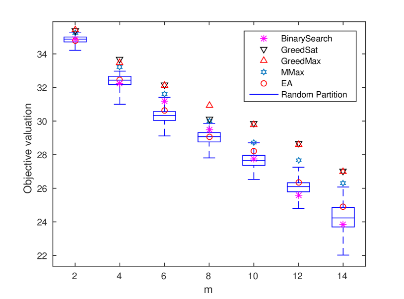
(a) Problem 1 on $f_{\text{fac}}$ with $\lambda=0$

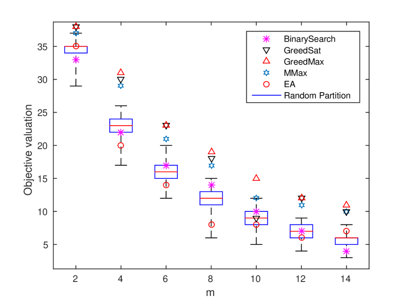
(b) Problem 1 on $f_{\text{sc}}$ with $\lambda=0$

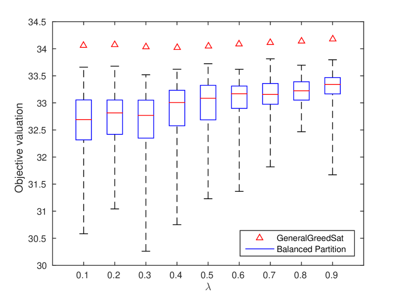
(c) Problem 1 on $f_{\text{fac}}$ with varying $\lambda$

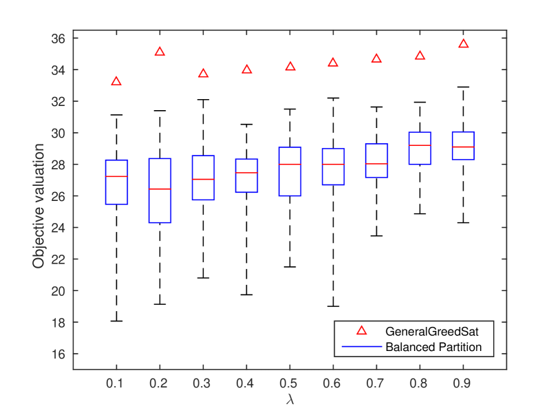
(d) Problem 1 on $f_{\text{sc}}$ with varying $\lambda$

Figure 2: Synthetic experiments on Problem 1 with $\lambda=0$ on facility location function (a) and set cover function (b). Problem 1 with general $0<\lambda<1$ on facility location function (c) and set cover function (d).

Problem 1

For $\lambda=0$, i.e., SFA, we compare among 6 algorithms: GreedMax, GreedSat, MMax, Balanced Partition (BP), Ellipsoid Approximation (EA) Goemans et al. (2009), and Binary Search algorithm (BS) Khot and Ponnuswami (2007). Balanced Partition method simply partitions the ground set $V$ into $m$ blocks such that the size of each block is balanced and is either $\lceil\frac{|V|}{m}\rceil$ or $\lfloor\frac{|V|}{m}\rfloor$. We run 100 randomly generated instances of the balanced partition method. GreedSat is implemented with the choice of the hyperparameter $\alpha=1$. We compare the performance of these algorithms in Figure 2(a) and 2(b), where we vary the number of blocks $m$ from 2 to 14. The three proposed algorithms (GreedMax, GreedSat, and MMax) significantly and consistently outperform all baseline methods for both $f_{\text{fac}}$ and $f_{\text{sc}}$. Among the proposed algorithms we observe that GreedMax, in general, yields the superior performance. Given the empirical success, computational efficiency, and tight theoretical guarantee, we suggest GreedMax as the first choice of algorithm to solve SFA under the homogeneous setting.

Next we evaluate Problem 1 with general $0<\lambda<1$. Baseline algorithms for SFA such as Ellipsoidal Approximations, Binary Search do not apply to the mixed scenario. Similarly the proposed algorithms such as GreedMax, MMax do not simply generalize to this scenario. We therefore only compare GeneralGreedSat with the Balanced Partition as a baseline. The results are summarized in Figure 2(c) and 2(d). We observe that GeneralGreedSat consistently and significantly outperform even the best of 100 instances of the baseline method for all cases of $\lambda$.

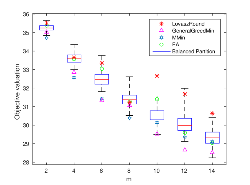
(a) Problem 2 on $f_{\text{fac}}$ with $\lambda=0$

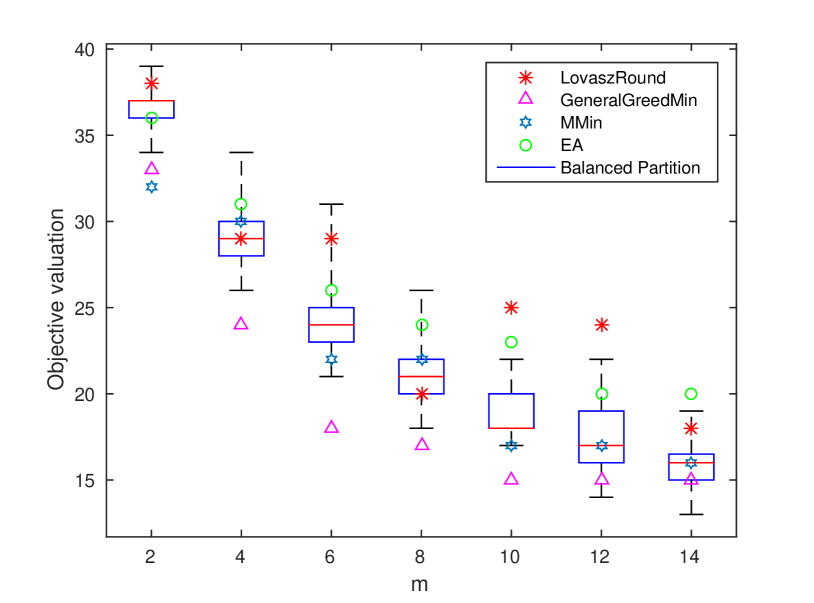
(b) Problem 2 on $f_{\text{sc}}$ with $\lambda=0$

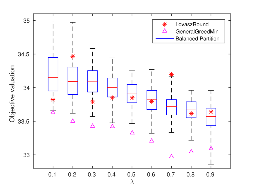
(c) Problem 2 on $f_{\text{fac}}$ with varying $\lambda$

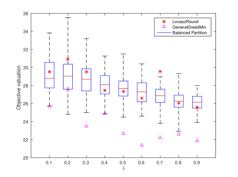
(d) Problem 2 on $f_{\text{sc}}$ with varying $\lambda$

Figure 3: Synthetic experiments on Problem 2 with $\lambda=0$ on facility location function (a) and set cover function (b). Problem 2 with general $0<\lambda<1$ on facility location function (c) and set cover function (d).

Problem 2

For $\lambda=0$, i.e., SLB, we compare among 5 algorithms: Lovász ​Round, MMin, GeneralGreedMin, Ellipsoid Approximation (EA) Goemans et al. (2009), and Balanced Partition Svitkina and Fleischer (2011). We implement GeneralGreedMin with the input argument $\lambda=0$. We also run $100$ randomly generated instances of the Balanced Partition method as a baseline. We show the results in Figure 3(a) and 3(b). Among all five algorithms MMin and GeneralGreedMin, in general, perform the best. Between MMin and GeneralGreedMin we observe that GeneralGreedMin performs marginally better, especially on $f_{\text{sc}}$. The computationally intensive algorithms, such as Ellipsoid Approximation and Lovász ​Round, do not perform well, though they carry better worst-case approximation factors for the heterogeneous setting.

Lastly we evaluate Problem 2 with general $0<\lambda<1$. Since MMin and Ellipsoid Approximation do not apply for the mixed scenario, we test only on GeneralLovász ​Round, GeneralGreedMin, and Balanced Partition. Again we test on 100 instances of randomly generated balanced partitions. We vary $\lambda$ in this experiment. The results are shown in Figure 3(c) and 3(d). The best performance is consistently achieved by GeneralGreedMin.

4.2 Problem 1 for Distributed Training

In this section we focus on applications of Problem 1 to real-wold machine learning problems. In particular we examine how a partition obtained by solving Problem 1 with certain instances of submodular functions perform for distributed training of various statistical models.

Distributed Convex Optimization:

We first consider data partitioning for distributed convex optimization. We evaluate the distributed convex optimization on a text categorization task. We use 20 Newsgroup data set , which consists of 18,774 articles divided almost evenly across 20 classes. The text categorization task is to classify an article into one newsgroup (of twenty) to which it was posted. We randomly split 2/3 and 1/3 of the whole data as the training and test data. The task is solved as a multi-class classification problem, which we formulate as an $\ell_{2}$ regularized logistic regression. We solve this convex optimization problem in a distributive fashion, where the data samples are partitioned and distributed across multiple machines. In particular we implement an ADMM algorithm as described in Boyd et al. (2011) to solve the distributed convex optimization problem. Given a partition $\pi$ of the training data into $m$ separate clients, in each iteration, ADMM first assigns each client $i$ to solve an $\ell_{2}$ regularized logistic regression on its block of data $A_{i}^{\pi}$ using L-BFGS, aggregate the solutions from all $m$ clients according to the ADMM update rules, and then sends the aggregated solution back to each client. This iterative procedure is carried out so that solutions on all clients converge to a consensus, which is the global solution of the overall large-scale convex optimization problem.

We formulate the data partitioning problem as an instance of SFA (Problem 1 with $\lambda=0$) under the homogeneous setting. In the experiment, we solve the data partitioning using GreedMax, since it is efficient and attains the tightest guarantee among all algorithms proposed for this setting. Note, however, GreedSat and MMax may also be used in the experiment. We model the utility of a data subset using the feature-based submodular function Wei et al. (2014b, 2015); Tschiatschek et al. (2014), which has the form:

$$f_{\text{fea}}(A)=\sum_{u\in\mathcal{U}}m_{u}(V)\log m_{u}(A),$$ (20)

where $\mathcal{U}$ is the set of “features”, $m_{u}(A)=\sum_{a\in A}m_{u}(a)$ with $m_{u}(a)$ measuring the degree that the article $a$ possesses the feature $u\in\mathcal{U}$. In the experiments, we define $\mathcal{U}$ as the set of all words occurred in the entire data set and $m_{u}(a)$ as the number of occurrences of the word $u\in\mathcal{U}$ in the article $a$. $f_{\text{fea}}$ is in the form of a sum of concave over modular functions, hence is monotone submodular Stobbe and Krause (2010). The class of feature-based submodular function has been widely applied to model the utility of a data subset on a number of tasks, including speech data subset selection Wei et al. (2014b, c), and image summarization Tschiatschek et al. (2014). Moreover $f_{\text{fea}}$ has been shown in Wei et al. (2015) to model the log-likelihood of a data subset for a Naïve Bayes classifier.

We compare the submodular partitioning with the random partitioning for $m=5$ and $m=10$. We test with $10$ instances of random partitioning. We first examine how balanced the sizes of the blocks yielded by submodular partitioning are. This is important since if the block sizes vary a lot in a partition, the computational loads across the blocks are imbalanced, and the actual efficiency of the parallel system is significantly reduced. Fortunately we observe that submodular partitioning yields very balanced partition. The sizes of all blocks in the resultant partitioning for $m=5$ range between $2,225$ and $2,281$. In the case of $m=10$ the maximum block is of size $1,140$, while the smallest block has $1,109$ items.

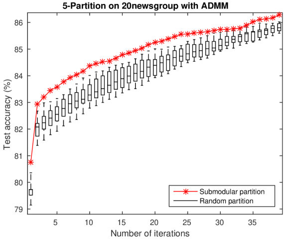
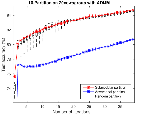
Figure 4: Distributed convex optimization tested on 20Newsgroups.

The comparison between submodular partitioning and random partitioning in terms of the accuracy of the model attained at any iteration is shown in Fig 4. For $m=10$ we also run an instance on an adversarial partitioning, where each block is formed by grouping every two of the 20 classes in the training data. We observe submodular partitioning converges faster than the random partitioning, both of which perform significantly better than the adversarial partition. In particular significant and consistent improvement over the best of 10 random instances is achieved by the submodular partition across all iterations when $m=5$.

Distributed Deep Neural Network Training: Next we evaluate our framework on distributed neural network training. We test on two tasks: 1) handwritten digit recognition on the MNIST database ; 2) phone classification on the TIMIT data.

The data for the handwritten digit recognition task consists of 60,000 training and 10,000 test samples. Each data sample is an image of handwritten digit. The training and test data are almost evenly divided into 10 different classes. For the phone classification task, the data consists of 1,124,823 training and 112,487 test samples. Each sample is a frame of speech. The training data is divided into 50 classes, each of which corresponds to a phoneme. The goal of this task to classify each speech sample into one of the 50 phone classes.

A $4$-layer DNN model is applied to the MNIST experiments, and we train a $5$-layered DNN for the TIMIT experiments. We apply the same distributed training procedure for both tasks. Given a partitioning of the training data, we distributively solve $m$ instances of sub-problems in each iteration. We define each sub-problem on a separate block of the data. We employ the stochastic gradient descent as the solver on each instance of the sub-problem. In the first iteration we use a randomly generated model as the initial model shared among the $m$ sub-problems. Each sub-problem is solved with $10$ epochs of the stochastic gradient decent training. We then average the weights in the $m$ resultant models to obtain a consensus model, which is used as the initial model for each sub-problem in the successive iteration. Note that this distributed training scheme is similar to the ones presented in Povey et al. (2014).

The submodular partitioning for both tasks is obtained by solving the homogeneous case of Problem 1 ($\lambda=0$) using GreedMax on a form of clustered facility location, as proposed and used in Wei et al. (2015). The function is defined as follows:

$$f_{\text{c-fac}}(A)=\sum_{y\in\mathcal{Y}}\sum_{v\in V^{y}}\max_{a\in A\cap V^{y}}s_{v,a}$$ (21)

where $s_{v,a}$ is the similarity measure between sample $v$ and $a$, $\mathcal{Y}$ is the set of class labels, and $V^{y}$ is the set of samples in $V$ with label $y\in\mathcal{Y}$. Note $\{V^{y}\}_{y\in\mathcal{Y}}$ forms a disjoint partitioning of the ground set $V$. In both the MNIST and TIMIT experiments we compute the similarity $s_{v,a}$ as the RBF kernel between the feature representation of $v$ and $a$.  Wei et al. (2015) show that $f_{\text{c-fac}}$ models the log-likelihood of a data subset for a Nearest Neighbor classifier. They also empirically demonstrate the efficacy of $f_{\text{c-fac}}$ in the case of neural network based classifiers.

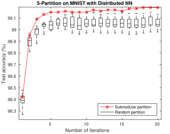
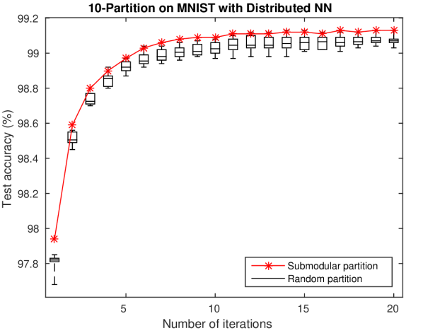
Figure 5: MNIST

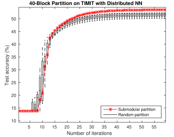
Figure 6: TIMIT

Similar to the ADMM experiment we also observe that submodular partitioning yields very balanced partitions in all cases of this experiment. In the cases of $m=5$ and $m=10$ for the MNIST data set the sizes of the blocks in the resultant submodular partitioning are within the range $[11991,12012]$ and $[5981,6019]$, respectively. For the TIMIT data set, the block sizes range between $37,483$ and $37510$ in the case of $m=30$, and the range of $[28121,28122]$ is observed for $m=40$.

We also run 10 instances of random partitioning as a baseline. The comparison between submodular partitioning and random partitioning in terms of the accuracy of the model attained at any iteration is shown in Fig 6 and 6. The adversarial partitioning, which is formed by grouping items with the same class, cannot even be trained in both cases. Consistent and significant improvement is again achieved by submodular partitioning for all cases.

4.3 Problem 2 for Unsupervised Image Segmentation

Lastly we test the efficacy of Problem 2 on the task of unsupervised image segmentation. We evaluate on the Grab-Cut data set, which consists of 30 color images. Each image has ground truth foreground/background labels. By “unsupervised”, we mean that no labeled data at any time in supervised or semi-supervised training, nor any kind of interactive segmentation, was used in forming or optimizing the objective. In our experiments, the image segmentation task is solved as unsupervised clustering of the pixels, where the goal is to obtain a partitioning of the pixels such that the majority of the pixels in each block share either the same foreground or the background labels.

Let $V$ be the ground set of pixels of an image, $\pi$ be an $m$-partition of the image, and $\{y_{v}\}_{v\in V}$ as the pixel-wise ground truth label ($y_{v}=\{0,1\}$ with 0 being background and 1 being foreground). We measure the performance of the partition $\pi$ in the following two steps: (1) for each block $i$, predict $\hat{y}_{v}$ for all the pixels $v\in A_{i}^{\pi}$ in the block as either $0$ or $1$ having larger intersection with the ground truth labels, i.e., predict $\hat{y}_{v}=1,\forall v\in A_{i}^{\pi}$, if $\sum_{v\in A_{i}^{\pi}}\mathbbm{1}\{y_{v}=1\}\geq\sum_{v\in A_{i}^{\pi}}\mathbbm{1}\{y_{v}=0\}$, and predict $\hat{y}_{v}=0,\forall v\in A_{i}^{\pi}$ otherwise. (2) report the performance of the partition $\pi$ as the F-measure of the predicted labels $\{\hat{y}_{v}\}_{v\in V}$ relative to the ground truth label $\{y_{v}\}_{v\in V}$.

In the experiment we first preprocess the data by downsampling each image by a factor $0.25$ for testing efficiency. We represent each pixel $v$ as 5-dimensional features $x_{v}\in\mathbb{R}^{5}$, including the RGB values and pixel positions. We normalize each feature within $[0,1]$. To obtain a segmentation of each image we solve an instance of Problem 2 ($0<\lambda<1$) under the homogeneous setting using GeneralGreedMin (Alg. 9). We use the facility location function $f_{\text{fac}}$ as the objective for Problem 2. The similarity $s_{v,a}$ between the pixels $v$ and $a$ is computed as $s_{v,a}=C-\|x_{v}-x_{a}\|_{2}$ with $C=\max_{v,v^{\prime}\in V}\|x_{v}-x_{v}^{\prime}\|_{2}$ being the maximum pairwise Euclidean distance. Since the facility location function $f_{\text{fac}}$ is defined on a pairwise similarity graph, which requires $O(|V|^{2})$ memory complexity. It becomes computationally infeasible for medium sized images. Fortunately a facility location function that is defined on a sparse $k$-nearest neighbor similarity graph performs just as well with $k$ being very sparse Wei et al. (2014a). In the experiment, we instantiate $f_{\text{fac}}$ by a sparse $10$-nearest neighbor sparse graph, where each item $v$ is connected only to its $10$ closest neighbors.

A number of unsupervised methods are tested as baselines in the experiment, including $k$-means, $k$-medoids, graph cuts Boykov and Kolmogorov (2004) and spectral clustering Von Luxburg (2007). We use the RBF kernel sparse similarity matrix as the input for spectral clustering. The sparsity of the similarity matrix is $k$ and the width parameter of the RBF kernel $\sigma$. We test with various choices of $\sigma$ and $k$ and find that the setting of $\sigma=1$ and $k=20$ performs the best, with which we report the results. For graph cuts, we use the MATLAB implementation Bagon (2006), which has a smoothness parameter $\alpha$. We tune $\alpha=0.3$ to achieve the best performance and report the result of graph cuts using this choice.

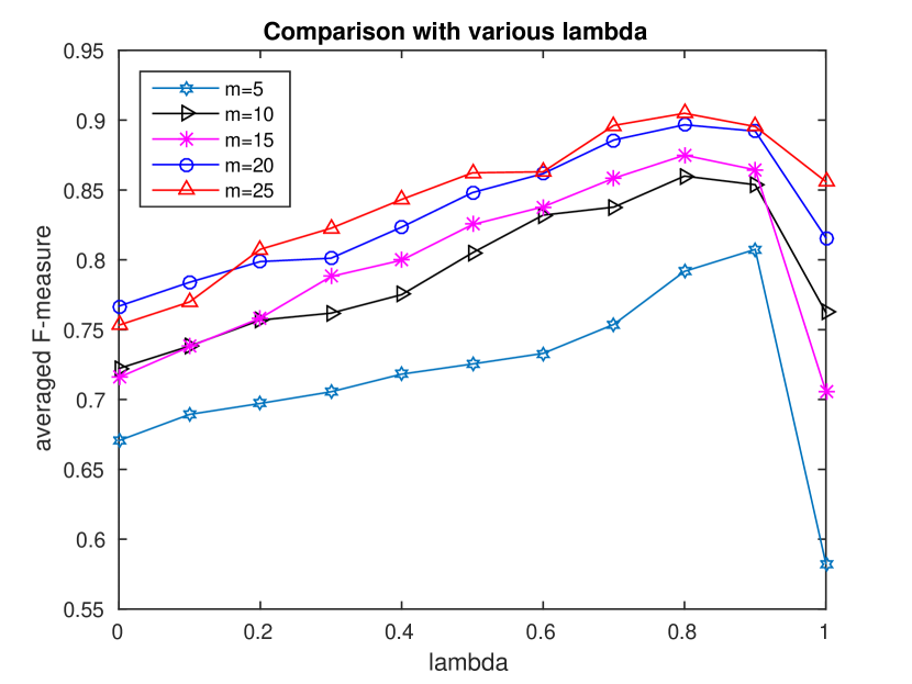
Figure 7: •

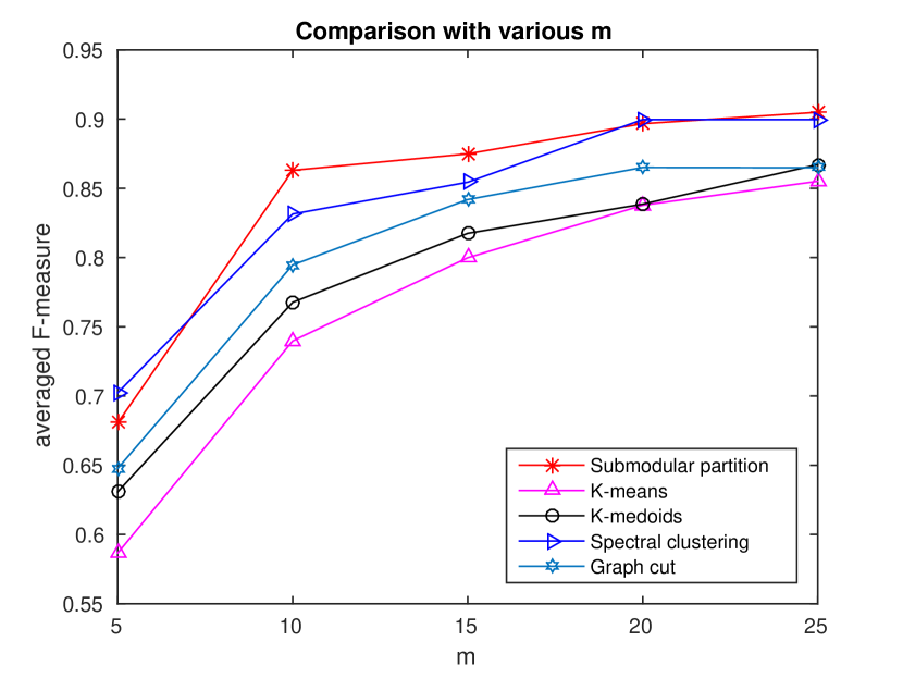
Figure 8:

The proposed image segmentation method involves a hyperparameter $\lambda$, which controls the trade-off between the worst-case objective and the average-case objective. First we examine how the performance of our method varies with different choices of $\lambda$ in Figure 8. The performance is measured as the averaged $F$-measure of a partitioning method over all images in the data set. Interestingly we observe that the performance smoothly varies as $\lambda$ increases from 0 to 1. In particular the best performance is achieved when $\lambda$ is within the range $[0.7,0.9]$. It suggests that using only the worst-case or the average-case objective does not suffice for the unsupervised image segmentation / clustering task, and an improved result is achieved by mixing these two extreme cases. In the subsequent experiments we show only the result of our method with $\lambda=0.2$. Next we compare the proposed approach with baseline methods on various $m$ in Figure 8. In general, each method improves as $m$ increases. Submodular partitioning method performs the best on almost all cases of $m$. Lastly we show in Figure 9 example segmentation results on several example images as well as averaged F-measure in the case of $m=15$. We observe that submodular partitioning, in general, leads to less noisy and more coherent segmentation in comparison to the baselines.

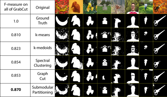
Figure 9: Unsupervised image segmentation (right: some examples).

5 Conclusions

In this paper, we considered two novel mixed robust/average-case submodular partitioning problems, which generalize four well-known problems: submodular fair allocation (SFA), submodular load balancing (SLB), submodular welfare problem (SWP), and submodular multiway partition (SMP). While the average case problems, i.e., SWP and SMP, admit efficient and tight algorithms, existing approaches for the worst case problems, i.e., SFA and SLB, are, in general, not scalable. We bridge this gap by providing several new algorithms that not only scale to large data sets but that also achieve comparable theoretical guarantees. Moreover we provide a number of efficient frameworks for solving the general mixed robust/average-case submodular partitioning problems. We also demonstrate that submodular partitioning is applicable in a number of machine learning problems involving distributed optimization, computational load balancing, and unsupervised image segmentation. Lastly we empirically show the effectiveness of the proposed algorithms on these machine learning tasks.

Acknowledgments

This material is based upon work supported by the National Science Foundation under Grant No. IIS-1162606, the National Institutes of Health under award R01GM103544, and by a Google, a Microsoft, and an Intel research award. R. Iyer acknowledges support from a Microsoft Research Ph.D Fellowship. This work was supported in part by TerraSwarm, one of six centers of STARnet, a Semiconductor Research Corporation program sponsored by MARCO and DARPA.

Appendix

Proof for Theorem 1

Theorem If $f_{1}$ and $f_{2}$ are monotone submodular, $\min\{f_{1}(A),f_{2}(V\setminus A)\}$ is also submodular.

Proof  To prove the Theorem, we show a more general result: Let $f$ and $h$ be submodular, and $f-h$ be either monotone increasing or decreasing, then $g(S)=\min\{f(S),h(S)\}$ is also submodular. The Theorem follows by this result, since $f(S)=f_{1}(S)$ and $h(S)=f_{2}(V\setminus S)$ are both submodular and $f(S)-h(S)=f_{1}(S)-f_{2}(V\setminus S)$ is monotone increasing.

In order to show $g$ is submodular, we prove that $g$ satisfies the following:

$$g(S)+g(T)\geq g(S\cap T)+g(S\cup T),\forall S,T\subseteq V$$ (22)

If $g$ agrees with either $f$ or $h$ on both $S$ and $T$, and since

$$f(S)+f(T)\geq f(S\cup T)+f(S\cap T)$$ (23)

$$h(S)+h(T)\geq h(S\cup T)+h(S\cap T),$$ (24)

Eqn 22 follows.

Otherwise, w.l.o.g. we consider $g(S)=f(S)$ and $g(T)=h(T)$. For the case where $f-h$ is monotone non-decreasing, consider the following:

$$g(S)+g(T) =f(S)+h(T)$$ (26)

$$\geq f(S\cup T)+f(S\cap T)-(f(T)-h(T))\mbox{ // submodularity of $f$}$$ (27)

$$\geq f(S\cup T)+f(S\cap T)-(f(S\cup T)-h(S\cup T))\mbox{ // monotonicity of $f-h$}$$ (28)

$$=f(S\cap T)+h(S\cup T)$$ (29)

$$\geq g(S\cap T)+g(S\cup T).$$ (30)

Similarly, for the case where $f-h$ is monotone non-increasing, consider the following:

$$g(S)+g(T) =f(S)+h(T)$$ (31)

$$\geq h(S\cap T)+h(S\cup T)+(f(S)-h(S))\mbox{ // submodularity of $h$}$$ (32)

$$\geq h(S\cup T)+h(S\cap T)+(f(S\cup T)-h(S\cup T))\mbox{ // monotonicity of $f-h$}$$ (33)

$$=h(S\cap T)+f(S\cup T)$$ (34)

$$\geq g(S\cap T)+g(S\cup T).$$ (35)

 

Proof for Theorem 2

Theorem Under the homogeneous setting ($f_{i}=f$ for all $i$), GreedMax is guaranteed to find a partition $\hat{\pi}$ such that

$$\min_{i=1,\dots,m}f(A_{i}^{\hat{\pi}})\geq\frac{1}{m}\max_{\pi\in\Pi}\min_{i=1,\dots,m}f(A_{i}^{\pi}).$$ (36)

Proof  We prove that the guarantee of $1/m$, in fact, even holds for a streaming version of the greedy algorithm (StreamGreed, see Alg. 10). In particular, we show that StreamGreed provides a factor of $1/m$ for SFA under the homogeneous setting. Theorem 2 then follows since GreedMax can be seen as running StreamGreed with a specific order.

Input: $V=\{v_{1},v_{2},\ldots,v_{n}\}$, $f$, $m$

Initialize: $A_{1}=,\dots,=A_{m}=\emptyset$, $k=1$

while $k\leq n$ do

       $i^{*}\in\operatorname*{argmin}_{j}f(A_{j})$

       $A_{i^{*}}\leftarrow A_{i^{*}}\cup\{v_{k}\}$

       $k\leftarrow k+1$

      

Algorithm 10 StreamGreed

To prove the guarantee for StreamGreed, we consider the resulting partitioning after an instance of StreamGreed: $\pi=(A^{\pi}_{1}\cup A^{\pi}_{2},\dots,A^{\pi}_{m})$. For simplicity of notation, we write $A_{i}^{\pi}$ as $A_{i}$ for each $i$ in the remaining proof. We refer $OPT$ to the optimal solution, i.e., $OPT=\max_{\pi}\min_{i}f(A_{i})$. W.l.o.g., we assume $f(A_{1})=\min_{i}f(A_{i})$. Let $a_{i}$ be the last item to be chosen in block $A_{i}$ for $i=2,\dots,m$.

Claim 1:

$$OPT\leq f(V\setminus\{a_{2},\dots,a_{m}\})$$ (37)

To show this claim, consider the following: If we enlarge the singleton value of $a_{i},i=2,\ldots,m$, we obtain a new submodular function:

$$f^{\prime}(A)=f(A)+\alpha\sum_{i=2}^{m}|A\cap a_{i}|,$$ (38)

where $\alpha$ is sufficiently large. Then running StreamGreed on $f^{\prime}$ with the same ordering of the incoming items leads to the same solution, since only the gain of the last added item for each block is changed.

Note that $f^{\prime}(A)\geq f(A),\forall A\subseteq V$, we then have $\max_{\pi}\min_{i}f^{\prime}(A_{i}^{\pi})\geq OPT$. The optimal partitioning for $f^{\prime}$ can be easily obtained as $\pi^{\prime}=(V\setminus\{a_{2},\dots,a_{m}\},a_{2},\dots,a_{m})$. Therefore, we have that

$$OPT\leq\max_{\pi}\min_{i}f^{\prime}(A_{i}^{\pi})=f^{\prime}(V\setminus\{a_{2},\dots,a_{m}\})=f(V\setminus\{a_{2},\dots,a_{m}\}).$$ (39)

Lastly, we have that $f(A_{1})\geq f(A_{i}\setminus a_{i})$ for any $i=2,\dots,m$ due to the procedure of StreamGreed. Therefore we have the following:

$$f(A_{1}) \geq\frac{1}{m}(f(A_{1})+\sum_{i=2}^{m}f(A_{i}\setminus a_{i}))$$ (40)

$$\geq\frac{1}{m}f(V\setminus\{a_{2},\dots,a_{m}\})\text{ // submodularity of $f$}$$ (41)

$$\geq\frac{1}{m}OPT\text{ // Claim 1}$$ (42)

 

Proof for Theorem 3

Theorem Given $\epsilon$, $\alpha$ and any $0<\delta<\alpha$, GreedSat finds a partition such that at least $\lceil m(\alpha-\delta)\rceil$ blocks receive utility at least $\frac{\delta}{1-\alpha+\delta}(\max_{\pi}\min_{i}f_{i}(A_{i}^{\pi})-\epsilon)$.

Proof  When GreedSat terminates, it identifies a $c_{\min}$ such that the returned solution $\hat{\pi}^{c_{\min}}$ satisfies $\bar{F}^{c_{\min}}(\hat{\pi}^{c_{\min}})\geq\alpha c_{\min}$. Also it identifies a $c_{\max}$ such that the returned solution $\hat{\pi}^{c_{\max}}$ satisfies $\bar{F}^{c_{\max}}(\hat{\pi}^{c_{\max}})<\alpha c_{\max}$. The gap between $c_{\max}$ and $c_{\min}$ is bounded by $\epsilon$, i.e., $c_{\max}-c_{\min}\leq\epsilon$.

Next, we prove that there does not exist any partitioning $\pi$ that satisfies $\min_{i}f_{i}(A_{i}^{\pi})\geq c_{\max}$, i.e., $c_{\max}\geq\max_{\pi\in\Pi}\min_{i}f_{i}(A_{i}^{\pi})$.

Suppose otherwise, i.e., $\exists\pi^{*}:\min_{i}f_{i}(A_{i}^{\pi^{*}})=c_{\max}+\gamma$ with $\gamma\geq 0$. Let $c=c_{\max}+\gamma$, consider the intermediate objective $\bar{F}^{c}(\pi)=\frac{1}{m}\sum_{i=1}^{m}\min\{f_{i}(A^{\pi}_{i}),c\}$, we have that $\bar{F}^{c}(\pi^{*})=c$. An instance of the algorithm for SWP on $\bar{F}^{c}$ is guaranteed to lead to a solution $\hat{\pi}^{c}$ such that $\bar{F}^{c}(\hat{\pi}^{c})\geq\alpha c$. Since $c\geq c_{\max}$, it should follow that the returned solution $\hat{\pi}^{c_{\max}}$ for the value $c_{\max}$ also satisfies $\bar{F}^{c_{\max}}(\hat{\pi})\geq\alpha c_{\max}$. However it contradicts with the termination criterion of GreedSat. Therefore, we prove that $c_{\max}\geq\max_{\pi\in\Pi}\min_{i}f_{i}(A_{i}^{\pi})$, which indicates that $c_{\min}\geq c_{\max}-\epsilon\geq\max_{\pi\in\Pi}\min_{i}f_{i}(A_{i}^{\pi})-\epsilon$.

Let $c^{*}=\frac{c_{\max}+c_{\min}}{2}$ and the partitioning returned by running for $c^{*}$ be $\hat{\pi}$ (the final output partitioning from GreedSat). We have that $\bar{F}^{c^{*}}(\hat{\pi})\geq\alpha c^{*}$, we are going to show that for any $0<\delta<\alpha$, at least a $\lceil m(\alpha-\delta)\rceil$ blocks given by $\hat{\pi}$ receive utility larger or equal to $\frac{\delta}{1-\alpha+\delta}c^{*}$.

Just to restate the problem: we say that the $i^{\text{th}}$ block is $(\alpha,\delta)$-good if $f_{i}(A_{i}^{\hat{\pi}})\geq\frac{\delta}{1-\alpha+\delta}c^{*}$. Then the statement becomes: Given $0<\delta<\alpha$, there is at least $m\lceil\alpha-\delta\rceil$ blocks that are $(\alpha,\delta)$-good.

To prove this statement, we assume, by contradiction, that there is strictly less than $\lceil m(\alpha-\delta)\rceil$ $(\alpha,\delta)$-good blocks. Denote the number of $(\alpha,\delta)$-good blocks as $m_{\text{good}}$. Then we have that $m_{\text{good}}\leq\lceil m(\alpha-\delta)\rceil-1<m(\alpha-\delta)$. Let $\theta=\frac{m_{\text{good}}}{m}$ be the fraction of $(\alpha,\delta)$ good blocks, then we have that $0\leq\theta<(\alpha-\delta)<1$. The remaining fraction $(1-\theta)$ of blocks are not good, i.e., they have valuation strictly less than $\frac{\delta}{1-\alpha+\delta}c^{*}$. Then, consider the following:

$$\bar{F}^{c^{*}}(\hat{\pi}) =\frac{1}{m}\sum_{i=1}^{m}\min\{f_{i}(A_{i}^{\hat{\pi}}),c^{*}\}$$ (43)

$$\stackrel{{\scriptstyle(a)}}{{<}}\theta c^{*}+(1-\theta)\frac{\delta}{1-\alpha+\delta}c^{*}$$ (44)

$$=\frac{\delta}{1-\alpha+\delta}c^{*}+\frac{1-\alpha}{1-\alpha+\delta}\theta c^{*}$$ (45)

$$\stackrel{{\scriptstyle(b)}}{{<}}\frac{\delta}{1-\alpha+\delta}c^{*}+\frac{1-\alpha}{1-\alpha+\delta}(\alpha-\delta)c^{*}$$ (46)

$$=\alpha c^{*}$$ (47)

Inequality (a) follows since good blocks are upper bounded by $c^{*}$, and not good blocks have values upper bounded by $\frac{\delta}{1-\alpha+\delta}c^{*}$. Inequality (b) follows by the assumption on $\theta$. This therefore contradicts the assumption that $\bar{F}^{c^{*}}(\hat{\pi})\geq\alpha c^{*}$, hence the statement is true.

This statement can also be proved using a different strategy. Let $f_{i}^{c^{*}}=\min\{f_{i}(A_{i}^{\hat{\pi}}),c^{*}\}$ and $f_{i}=f_{i}(A_{i}^{\hat{\pi}})$ for all $i$. For any $0\leq\beta\leq 1$ the following holds:

$$\alpha c^{*}\leq\bar{F}^{c^{*}}(\hat{\pi})=\frac{1}{m}\sum_{i}f^{c^{*}}_{i}\leq\frac{1}{m}f_{i}=\frac{1}{m}\sum_{i:f_{i}<\beta c^{*}}f_{i}+\frac{1}{m}\sum_{i:f_{i}\geq\beta c^{*}}f_{i}<\frac{1}{m}m_{\text{bad}}\beta c^{*}+\frac{1}{m}m_{\text{good}}c^{*}$$ (48)

where $m=m_{\text{bad}}+m_{\text{good}}$ and $m_{\text{good}}$ are the number that are $\beta$-good (i.e., $i$ is $\beta$-good if $f_{i}\geq\beta c^{*}$). The goal is to place a lower bound on $m_{\text{good}}$. From the above

$$\alpha<(1-\frac{m_{\text{good}}}{m})\beta+\frac{m_{\text{good}}}{m}$$ (49)

which means

$$m_{\text{good}}\geq\lceil\frac{\alpha-\beta}{1-\beta}m\rceil$$ (50)

Let $\beta=\frac{\delta}{1-\alpha+\delta}$, the statement immediately follows.

Note $c^{*}=\frac{c_{\min}+c_{\max}}{2}\geq c_{\max}-\epsilon\geq\max_{\pi\in\Pi}\min_{i}f_{i}(A_{i}^{\pi})-\epsilon$. Combining pieces together, we have shown that at least $\lceil m(\alpha-\delta)\rceil$ blocks given by $\hat{\pi}$ receive utility larger or equal to $\frac{\delta}{1-\alpha+\delta}(\max_{\pi\in\Pi}\min_{i}f_{i}(A_{i}^{\pi})-\epsilon)$.  

Proof for Theorem 4

Theorem MMax achieves a worst-case guarantee of $O(\min_{i}\frac{1+(|{A}^{\hat{\pi}}_{i}|-1)(1-\kappa_{f_{i}}({A}^{\hat{\pi}}_{i}))}{|{A}^{\hat{\pi}}_{i}|\sqrt{m}\log^{3}m})$, where $\hat{\pi}=({A^{\hat{\pi}}_{1}},\cdots,A^{\hat{\pi}}_{m})$ is the partition obtained by the algorithm, and $\kappa_{f}(A)=1-\min_{v\in V}\frac{f(v|A\setminus v)}{f(v)}\in[0,1]$ is the curvature of a submodular function $f$ at $A\subseteq V$.

Proof  We assume the approximation factor of the algorithm for solving the modular version of Problem 1 is $\alpha=O(\frac{1}{\sqrt{m}\log^{3}m})$ Asadpour and Saberi (2010). For notation simplicity, we write $\hat{\pi}=(\hat{A}_{1},\dots,\hat{A}_{m})$ as the resulting partition after the first iteration of MMax, and $\pi^{*}=(A_{1}^{*},\dots,A_{m}^{*})$ as its optimal solution. Note that first iteration suffices to yield the performance guarantee, and the subsequent iterations are designed so as to improve the empirical performance. Since the proxy function for each function $f_{i}$ used for the first iteration are the simple modular upper bound with the form: $h_{i}(X)=\sum_{j\in X}f_{i}(j)$.

Given the curvature of each submodular function $f_{i}$, we can tightly bound a submodular function $f_{i}$ in the following form Iyer et al. (2013b):

$$f_{i}(X)\leq h_{i}(X)\leq\frac{|X|}{1+(|X|-1)(1-\kappa_{f_{i}}(X))}f_{i}(X),\forall X\subseteq V$$ (51)

Consider the following:

$$\min_{i}f_{i}(\hat{A}_{i}) \geq\min_{i}\frac{1}{\frac{|\hat{A}_{i}|}{1+(|\hat{A}_{i}|-1)(1-\kappa_{f_{i}}(\hat{A}_{i}))}}h_{i}(\hat{A}_{i})$$ (52)

$$\geq\min_{i}\frac{1}{\frac{|\hat{A}_{i}|}{1+(|\hat{A}_{i}|-1)(1-\kappa_{f_{i}}(\hat{A}_{i}))}}\min_{i}h_{i}(\hat{A}_{i})$$ (53)

$$\geq\alpha\min_{i}\frac{1+(|\hat{A}_{i}|-1)(1-\kappa_{f_{i}}(\hat{A}_{i}))}{|\hat{A}_{i}|}\min_{i}h_{i}(A_{i}^{*})$$ (54)

$$\geq\alpha\min_{i}\frac{1+(|\hat{A}_{i}|-1)(1-\kappa_{f_{i}}(\hat{A}_{i}))}{|\hat{A}_{i}|}\min_{i}f_{i}(A_{i}^{*})$$ (55)

$$=O(\min_{i}\frac{1+(|\hat{A}_{i}|-1)(1-\kappa_{f_{i}}(\hat{A}_{i}))}{|\hat{A}_{i}|\sqrt{m}\log^{3}m})\min_{i}f_{i}(A^{*}_{i}).$$ (56)

 

Proof for Theorem 5

Theorem Suppose there exists an algorithm for solving the modular version of SFA with an approximation factor $\alpha\leq 1$, we have that

$$\min_{i}f_{i}(A_{i}^{\pi_{t}})\geq\alpha\min_{i}f_{i}(A_{i}^{\pi_{t-1}}).$$ (57)

Proof  Consider the following:

$$\min_{i}f_{i}(A^{\pi_{t-1}}_{i}) =\min_{i}h_{i}(A^{\pi_{t-1}}_{i})//\mbox{ tightness of modular lower bound.}$$ (58)

$$\leq\alpha\min_{i}h_{i}(A_{i}^{\pi_{t}})//\mbox{ approximation factor of the modular SFA. }$$ (59)

$$\leq\alpha h_{j}(A_{j}^{\pi_{t}})//j\in\operatorname*{argmin}_{i}f_{i}(A_{i}^{\pi_{t}})$$ (60)

$$\leq\alpha f_{j}(A_{j}^{\pi_{t}})//h_{j}(A_{j}^{\pi_{t-1}})\mbox{ upper bounds }f_{j}\mbox{ everywhere.}$$ (61)

$$=\alpha\min_{i}f_{i}(A_{i}^{\pi_{t}})$$ (62)

 

Proof for Theorem 6

Theorem For any $\epsilon>0$, SLB cannot be approximated to a factor of $(1-\epsilon)m$ for any $m=o(\sqrt{n/\log n})$ with polynomial number of queries even under the homogeneous setting.

Proof  We use the same proof techniques as in Svitkina and Fleischer (2008). Consider two submodular functions:

$$f_{1}(S)=\min\{|S|,\alpha\};$$ (63)

$$f_{2}(S)=\min\{\sum_{i=1}^{m}\min\{\beta,|S\cap V_{i}|\},\alpha\};$$ (64)

where $\{V_{i}\}_{i=1}^{m}$ is a uniformly random partitioning of $V$ into $m$ blocks, $\alpha=\frac{n}{m}$ and $\beta=\frac{n}{m^{2}(1-\epsilon)}$. To be more precise about the uniformly random partitioning, we assign each item into any one of the $m$ blocks with probability $1/m$. It can be easily verified that $OPT_{1}=\min_{\pi\in\Pi}\max_{i}f_{1}(A_{i}^{\pi})=n/m$ and $OPT_{2}=\min_{\pi\in\Pi}\max_{i}f_{2}(A_{i}^{\pi})=\frac{n}{m^{2}(1-\epsilon)}$. The gap is then $\frac{OPT_{1}}{OPT_{2}}=m(1-\epsilon)$.

Next, we show that $f_{1}$ and $f_{2}$ cannot be distinguished with $n^{\omega(1)}$ number of queries.

Since $f_{1}(S)\geq f_{2}(S)$ holds for any $S$, this is equivalent as showing $P\{f_{1}(S)>f_{2}(S)\}<n^{-\omega(1)}$.

As shown in Svitkina and Fleischer (2008), $P\{f_{1}(S)>f_{2}(S)\}$ is maximized when $|S|=\alpha$. It suffices to consider only the case of $|S|=\alpha$ as follows:

$$P\{f_{1}(S)>f_{2}(S):|S|=\alpha\}=P\{\sum_{i=1}^{m}\min\{\beta,|S\cap V_{i}|\}<\alpha:|S|=\alpha\}$$ (65)

The necessary condition for $\sum_{i=1}^{m}\min\{\beta,|S\cap V_{i}|\}<\alpha$ is that $|S\cap V_{i}|>\beta$ is satisfied for some $i$. Using the Chernoff bound, we have that for any $i$, it holds $P\{|S\cap V_{i}|>\beta\}\leq e^{-\frac{\epsilon^{2}n}{3m^{2}}}=n^{-\omega(1)}$ when $m=o(\sqrt{n/\log n})$. Using the union bound, it holds that the probability for any one block $V_{i}$ such that $|S\cap V_{i}|>\beta$ is also upper bounded by $n^{-\omega(1)}$. Combining all pieces together, we have the following:

$$P\{f_{1}(S)>f_{2}(S)\}\leq n^{-\omega(1)}.$$ (66)

Finally, we come to prove the Theorem. Suppose the goal is to solve an instance of SLB with $f_{2}$. Since $f_{1}$ and $f_{2}$ are hard to distinguish with polynomial number of function queries, any polynomial time algorithm for solving $f_{2}$ is equivalent to solving for $f_{1}$. However, the optimal solution for $f_{1}$ is $\alpha=\frac{n}{m}$, whereas the optimal solution for $f_{2}$ is $\beta=\frac{n}{m^{2}(1-\epsilon)}$. Therefore, no polynomial time algorithm can find a solution with a factor $m(1-\epsilon)$ for SLB in this case.  

Proof for Theorem 7

Theorem LovászRound is guaranteed to find a partition $\hat{\pi}\in\Pi$ such that $\max_{i}f_{i}(A_{i}^{\hat{\pi}})\leq m\min_{\pi\in\Pi}\max_{i}f_{i}(A_{i}^{\pi})$.

Proof  It suffices to bound the performance loss at the step of rounding the fractional solution $\{x^{*}_{i}\}_{i=1}^{m}$, or equivalently, the following:

$$\max_{i}\tilde{f}_{i}(x_{i}^{*})\geq\frac{1}{m}\max_{i}f_{i}(A_{i}),$$ (67)

where $\{A_{i}\}_{i=1}^{m}$ is the resulting partitioning after the rounding. To show Eqn 67, it suffices to show that $\tilde{f}_{i}(x_{i}^{*})\geq\frac{1}{m}f_{i}(A_{i})$ for all $i=1,\dots,m$. Next, consider the following:

$$f_{i}(A_{i}) =\tilde{f}_{i}(1_{A_{i}})=m\tilde{f}_{i}(\frac{1}{m}1_{A_{i}})//\mbox{ positive homogeneity of Lov\'{a}sz {} extension}$$ (68)

For any item $v_{j}\in A_{i}$, we have $x^{*}_{i}(j)\geq\frac{1}{m}$, since $\sum_{i=1}^{m}x^{*}_{i}(j)\geq 1$ and $x^{*}_{i}(j)=\max_{i^{\prime}}x_{i^{\prime}}(j)$. Therefore, we have $\frac{1}{m}1_{A_{i}}\leq x_{i}^{*}$. Since $f_{i}$ is monotone, its extension $\tilde{f}_{i}$ is also monotone. As a result, $f_{i}(A_{i})=m\tilde{f}_{i}(\frac{1}{m}1_{A_{i}})\leq m\tilde{f}_{i}(x_{i}^{*})$.

 

Proof for Theorem 8

Theorem MMin achieves a worst-case guarantee of $(2\max_{i}\frac{|A_{i}^{\pi^{*}}|}{1+(|A_{i}^{\pi^{*}}|-1)(1-\kappa_{f_{i}}(A_{i}^{\pi^{*}}))})$, where $\pi^{*}=(A_{1}^{\pi^{*}},\cdots,A_{m}^{\pi^{*}})$ denotes the optimal partition.

Proof  Let $\alpha=2$ be the approximation factor of the algorithm for solving the modular version of Problem 2 Lenstra et al. (1990). For notation simplicity, we write $\hat{\pi}=(\hat{A}_{1},\dots,\hat{A}_{m})$ as the resulting partition after the first iteration of MMin, and $\pi^{*}=(A_{1}^{*},\dots,A_{m}^{*})$ as its optimal solution. Again the first iteration suffices to yield the performance guarantee, and the subsequent iterations are designed so as to improve the empirical performance. Since the supergradients for each function $f_{i}$ used for the first iteration are the simple modular upper bound with the form: $h_{i}(X)=\sum_{j\in X}f_{i}(j)$, we can again tightly bound a submodular function $f_{i}$ in the following form:

$$f_{i}(X)\leq h_{i}(X)\leq\frac{|X|}{1+(|X|-1)(1-\kappa_{f_{i}}(X))}f_{i}(X),\forall X\subseteq V$$ (69)

Consider the following:

$$\max_{i}f_{i}(\hat{A}_{i}) \leq\max_{i}h_{i}(\hat{A}_{i})$$ (70)

$$\leq\alpha\max_{i}h_{i}(A_{i}^{*})$$ (71)

$$\leq\alpha\max_{i}\frac{|A_{i}^{*}|}{1+(|A_{i}^{*}|-1)(1-\kappa_{f_{i}}(A_{i}^{*}))}f_{i}(A_{i}^{*})$$ (72)

$$\leq\alpha\max_{i}\frac{|A_{i}^{*}|}{1+(|A_{i}^{*}|-1)(1-\kappa_{f_{i}}(A_{i}^{*}))}\max_{i}f_{i}(A_{i}^{*})$$ (73)

 

Proof for Theorem 9

Theorem Suppose there exists an algorithm for solving the modular version of SLB with an approximation factor $\alpha\geq 1$, we have for each iteration $t$ that

$$\max_{i}f_{i}(A_{i}^{\pi_{t}})\leq\alpha\max_{i}f_{i}(A_{i}^{\pi_{t-1}}).$$ (74)

Proof  The proof is symmetric to the one for Theorem 5.  

Proof for Theorem 10

We prove separately for Problem 1 and Problem 2.

Theorem Given an instance of Problem 1 with $0<\lambda<1$, CombSfaSwp provides an approximation guarantee of $\max\{\min\{\alpha,\frac{1}{m}\},\frac{\beta\alpha}{\bar{\lambda}\beta+\alpha},\lambda\beta\}$ in the homogeneous case, and a factor of $\max\{\frac{\beta\alpha}{\bar{\lambda}\beta+\alpha},\lambda\beta\}$ in the heterogeneous case, where $\alpha$ and $\beta$ are the approximation factors of AlgWC and AlgAC for SFA and SWP respectively.

Proof  We first prove the result for heterogeneous setting. For notation simplicity we write the worst-case objective as $F_{1}(\pi)=\min_{i=1,\ldots,m}f(A_{i}^{\pi})$ and the average-case objective as $F_{2}(\pi)=\frac{1}{m}\sum_{i=1,\ldots,m}f(A_{i}^{\pi})$.

Suppose AlgWC outputs a partition $\hat{\pi}_{1}$ and AlgAC outputs a partition $\hat{\pi}_{2}$. Let $\pi^{*}\in\arg\max_{\pi\in\Pi}\bar{\lambda}F_{1}(\pi)+\lambda F_{2}(\pi)$ be the optimal partition.

We use the following facts:

Fact1

$$F_{1}(\hat{\pi}_{1})\geq\alpha F_{1}(\pi)$$ (75)

Fact2

$$F_{2}(\pi_{2})\geq\beta F_{2}(\pi)$$ (76)

Fact3

$$F_{1}(\pi) \leq F_{2}(\pi)$$ (77)

Then we have that

$$\bar{\lambda}F_{1}(\hat{\pi}_{2})+\lambda F_{2}(\hat{\pi}_{2}) \geq\lambda F_{2}(\hat{\pi}_{2})$$ (78)

$$\geq\lambda\beta F_{2}(\pi^{*})$$ (79)

$$\geq\lambda\beta\left[\bar{\lambda}F_{1}(\pi^{*})+\lambda F_{2}(\pi^{*})\right]$$ (80)

and

$$\bar{\lambda}F_{1}(\hat{\pi}_{1})+\lambda F_{2}(\hat{\pi}_{1}) \geq\mu\left[\bar{\lambda}F_{1}(\hat{\pi}_{1})+\lambda F_{2}(\hat{\pi}_{1})\right]+(1-\mu)\left[\bar{\lambda}F_{1}(\hat{\pi}_{1})+\lambda F_{2}(\hat{\pi}_{1})\right]$$ (81)

$$\geq\mu\left[\bar{\lambda}\alpha F_{1}(\pi^{*})+\lambda\alpha F_{1}(\pi^{*})\right]+(1-\mu)\left[0+\lambda\beta F_{2}(\pi^{*})\right]$$ (82)

$$\geq\frac{\mu\alpha}{\bar{\lambda}}\bar{\lambda}F_{1}(\pi^{*})+(1-\mu)\beta\lambda F_{2}(\pi^{*})$$ (83)

$$\geq\min\{\frac{\mu\alpha}{\bar{\lambda}},(1-\mu)\beta\}\left[\bar{\lambda}F_{1}(\pi^{*})+\lambda F_{2}(\pi^{*})\right]$$ (84)

$\min\{\frac{\mu\alpha}{\bar{\lambda}},(1-\mu)\beta\}$ is a function over $0\leq\mu\leq 1$ and $\mu^{*}\in\arg\max_{\mu}\min\{\frac{\mu\alpha}{\bar{\lambda}},(1-\mu)\beta\}$. It is easy to show

$$\mu^{*} =\frac{\bar{\lambda}\beta}{\bar{\lambda}\beta+\alpha}$$ (85)

$$\max_{\mu}\min\{\frac{\mu\alpha}{\bar{\lambda}},(1-\mu)\beta\} =\frac{\beta\alpha}{\bar{\lambda}\beta+\alpha}$$ (86)

$$\bar{\lambda}F_{1}(\hat{\pi}_{1})+\lambda F_{2}(\hat{\pi}_{1})\geq\frac{\beta\alpha}{\bar{\lambda}\beta+\alpha}\left[\bar{\lambda}F_{1}(\pi^{*})+\lambda F_{2}(\pi^{*})\right]$$ (87)

Taking the max over the two bounds leads to

$$\max\{\bar{\lambda}F_{1}(\hat{\pi}_{1})+\lambda F_{2}(\hat{\pi}_{1}),\bar{\lambda}F_{1}(\hat{\pi}_{2})+\lambda F_{2}(\hat{\pi}_{2})\}\geq\max\{\frac{\beta\alpha}{\bar{\lambda}\beta+\alpha},\lambda\beta\}\max_{\pi\in\Pi}\bar{\lambda}F_{1}(\pi)+\lambda F_{2}(\pi)$$ (88)

Next we are going to show the result for the homogeneous setting. We have the following facts that hold for arbitrary partition $\pi$:

$$F_{1}(\hat{\pi}_{1}) \geq\alpha F_{1}(\pi),\ F_{2}(\hat{\pi}_{2})\geq\beta F_{2}(\pi)$$ (89)

$$F_{1}(\pi) \leq F_{2}(\pi),\ F_{2}(\pi_{1})\geq\frac{1}{m}F_{2}(\pi)$$ (90)

Consider the following:

$$\bar{\lambda}F_{1}(\hat{\pi}_{1})+\lambda F_{2}(\hat{\pi}_{1}) \geq\alpha\bar{\lambda}F_{1}({\pi}^{*})+\frac{\lambda}{m}F_{2}({\pi}^{*})$$ (91)

$$\geq\min\{\alpha,\frac{1}{m}\}\left[\bar{\lambda}F_{1}({\pi}^{*})+\lambda F_{2}({\pi}^{*})\right]$$ (92)

and

$$\bar{\lambda}F_{1}(\hat{\pi}_{2})+\lambda F_{2}(\hat{\pi}_{2}) \geq\lambda F_{2}(\hat{\pi}_{2})$$ (93)

$$\geq\lambda\beta F_{2}(\pi^{*})$$ (94)

$$\geq\lambda\beta\left[\bar{\lambda}F_{1}(\pi^{*})+\lambda F_{2}(\pi^{*})\right]$$ (95)

Taking the max over the two bounds and the result shown in Eqn 87 gives the following:

$$\max\{\bar{\lambda}F_{1}(\hat{\pi}_{1})+\lambda F_{2}(\hat{\pi}_{1}),\bar{\lambda}F_{1}(\hat{\pi}_{2})+\lambda F_{2}(\hat{\pi}_{2})\}\geq\max\{\min\{\alpha,\frac{1}{m}\},\frac{\beta\alpha}{\bar{\lambda}\beta+\alpha},\lambda\beta\}\max_{\pi\in\Pi}\bar{\lambda}F_{1}(\pi)+\lambda F_{2}(\pi).$$ (96)

 

Theorem CombSlbSmp provides an approximation guarantee of $\min\{m,\frac{m\alpha}{m\bar{\lambda}+\lambda},\beta(m\bar{\lambda}+\lambda)\}$ in the homogeneous case, and a factor of $\min\{\frac{m\alpha}{m\bar{\lambda}+\lambda},\beta(m\bar{\lambda}+\lambda)\}$ in the heterogeneous case, for Problem 2 with $0\leq\lambda\leq 1$.

Proof  Let $\hat{\pi}_{1}$ be the solution of AlgWC and $\hat{\pi}_{2}$ be the solution of AlgAC. Let $\pi^{*}\in\arg\min_{\pi\in\Pi}\bar{\lambda}F_{1}(\pi)+\lambda F_{2}(\pi)$ be the optimal partition. The following facts hold for all $\pi\in\Pi$:

Fact1

$$F_{1}(\hat{\pi}_{1})\leq\alpha F_{1}(\pi)$$ (97)

Fact2

$$F_{2}(\hat{\pi}_{2})\leq\beta F_{2}(\pi)$$ (98)

Fact3

$$F_{2}(\pi)\leq F_{1}(\pi)\leq mF_{2}(\pi)$$ (99)

Then we have the following:

$$\bar{\lambda}F_{1}(\hat{\pi}_{1})+\lambda F_{2}(\hat{\pi}_{1}) \leq F_{1}(\hat{\pi}_{1})$$ (100)

$$\leq\alpha F_{1}(\pi^{*})$$ (101)

$$\leq\frac{\alpha}{\bar{\lambda}+\frac{\lambda}{m}}\left[\bar{\lambda}F_{1}(\pi^{*})+\frac{\lambda}{m}F_{1}(\pi^{*})\right]$$ (102)

$$\leq\frac{m\alpha}{m\bar{\lambda}+\lambda}\left[\bar{\lambda}F_{1}(\pi^{*})+\lambda F_{2}(\pi^{*})\right]$$ (103)

and

$$\bar{\lambda}F_{1}(\hat{\pi}_{2})+\lambda F_{2}(\hat{\pi}_{2}) \leq\beta m\bar{\lambda}F_{2}(\pi^{*})+\beta\lambda F_{2}(\pi^{*})$$ (104)

$$\leq(m\bar{\lambda}+\lambda)\beta F_{2}(\pi^{*})$$ (105)

$$\leq(m\bar{\lambda}+\lambda)\beta\left[\bar{\lambda}F_{1}(\pi^{*})+\lambda F_{2}(\pi^{*})\right]$$ (106)

Taking the minimum over the two leads to the following:

$$\min\{\bar{\lambda}F_{1}(\hat{\pi}_{1})+\lambda F_{2}(\hat{\pi}_{1}),\bar{\lambda}F_{1}(\hat{\pi}_{2})+\lambda F_{2}(\hat{\pi}_{2})\}\leq\min\{\frac{m\alpha}{m\bar{\lambda}+\lambda},\beta(m\bar{\lambda}+\lambda)\}\min_{\pi\in\Pi}\bar{\lambda}F_{1}(\pi)+\lambda F_{2}(\pi)$$ (108)

Equation 108 gives us a bound for both the homogeneous setting and the heterogeneous settings.

Furthermore, in the homogeneous setting, for arbitrary partition $\pi$, we have

$$\bar{\lambda}F_{1}({\pi})+\lambda F_{2}({\pi})\leq m\min_{\pi\in\Pi}\bar{\lambda}F_{1}(\pi)+\lambda F_{2}(\pi)$$ (109)

and we can tighten the bound for the homogeneous setting as follows:

$$\min\{\bar{\lambda}F_{1}(\hat{\pi}_{1})+\lambda F_{2}(\hat{\pi}_{1}),\bar{\lambda}F_{1}(\hat{\pi}_{2})+\lambda F_{2}(\hat{\pi}_{2})\} \leq\min\{m,\frac{m\alpha}{m\bar{\lambda}+\lambda},\beta(m\bar{\lambda}+\lambda)\}\max_{\pi\in\Pi}\bar{\lambda}F_{1}(\pi)+\lambda F_{2}(\pi)$$ (110)

 

Proof for Theorem 11

Theorem Given $\epsilon$, $\alpha$, and, $0\leq\lambda\leq 1$, GeneralGreedSat finds a partition $\hat{\pi}$ that satisfies the following:

$$\bar{\lambda}\min_{i}f_{i}(A_{i}^{\hat{\pi}})+\lambda\frac{1}{m}\sum_{i=1}^{m}f_{i}(A_{i}^{\hat{\pi}})\geq\lambda\alpha(OPT-\epsilon),$$ (111)

where $OPT=\max_{\pi\in\Pi}\bar{\lambda}\min_{i}f_{i}(A_{i}^{\pi})+\lambda\frac{1}{m}\sum_{i=1}^{m}f_{i}(A_{i}^{\pi})$.

Moreover, let $F_{\lambda,i}(\pi)=\bar{\lambda}f_{i}(A_{i}^{\pi})+\lambda\frac{1}{m}\sum_{j=1}^{m}f_{j}(A_{j}^{\pi})$. Given any $0<\delta<\alpha$, there is a set $I\subseteq\{1,\dots,m\}$ such that $|I|\geq\lceil m(\alpha-\delta)\rceil$ and

$$F_{i,\lambda}(\hat{\pi})\geq\max\{\frac{\delta}{1-\alpha+\delta},\lambda\alpha\}(OPT-\epsilon),\forall i\in I.$$ (112)

Proof  Denote intermediate objective $\bar{F}^{c}(\pi)=\frac{1}{m}\sum_{i=1}^{m}\min\{\bar{\lambda}f_{i}(A_{i}^{{\pi}})+\lambda\frac{1}{m}\sum_{j=1}^{m}f_{j}(A_{j}^{{\pi}}),c\}$. Also we define the overall objective as $F(\pi)=\bar{\lambda}\min_{i}f_{i}(A_{i}^{\pi})+\lambda\frac{1}{m}\sum_{i=1}^{m}f_{i}(A_{i}^{\pi})$. When the algorithm terminates, it identifies a $c_{\min}$ such that the returned solution $\hat{\pi}^{c_{\min}}$ satisfies $\bar{F}^{c_{\min}}(\hat{\pi}^{c_{\min}})\geq\alpha c_{\min}$. Also it identifies a $c_{\max}$ such that the returned solution $\hat{\pi}^{c_{\max}}$ satisfies $\bar{F}^{c_{\max}}(\hat{\pi}^{c_{\max}})<\alpha c_{\max}$. The gap between $c_{\max}$ and $c_{\min}$ is bounded by $\epsilon$, i.e., $c_{\max}-c_{\min}\leq\epsilon$.

Next, we prove that there does not exist any partitioning $\pi$ that satisfies $F(\pi)\geq c_{\max}$, i.e., $c_{\max}\geq OPT$.

Suppose otherwise, i.e., $\exists\pi^{*}:F(\pi^{*})=c_{\max}+\gamma$ with $\gamma\geq 0$. Let $c=c_{\max}+\gamma$, consider the intermediate objective $\bar{F}^{c}(\pi)$, we have that $\bar{F}^{c}(\pi^{*})=c$. An instance of the algorithm for SWP on $\bar{F}^{c}$ is guaranteed to lead to a solution $\hat{\pi}^{c}$ such that $\bar{F}^{c}(\hat{\pi}^{c})\geq\alpha c$. Since $c\geq c_{\max}$, it should follow that the returned solution $\hat{\pi}^{c_{\max}}$ for the value $c_{\max}$ also satisfies $\bar{F}^{c_{\max}}(\hat{\pi})\geq\alpha c_{\max}$. However it contradicts with the termination criterion of GreedSat. Therefore, we prove that $c_{\max}\geq OPT$, which indicates that $c_{\min}\geq c_{\max}-\epsilon\geq OPT-\epsilon$.

Let $c^{*}=\frac{c_{\max}+c_{\min}}{2}$ and the partitioning returned by running for $c^{*}$ be $\hat{\pi}$ (the final output partitioning from the algorithm). We have that $\bar{F}^{c^{*}}(\hat{\pi})\geq\alpha c^{*}$.

Next we are ready to prove the Theorem: $F(\hat{\pi})\geq\lambda\alpha$. For simplicity of notation, we rewrite $y_{i}=\bar{\lambda}f_{i}(A_{i}^{\hat{\pi}})+\lambda\frac{1}{m}\sum_{j=1}^{m}f_{j}(A_{j}^{\hat{\pi}})$ and $x_{i}=\min\{\bar{\lambda}f_{i}(A_{i}^{\hat{\pi}})+\lambda\frac{1}{m}\sum_{j=1}^{m}f_{j}(A_{j}^{\hat{\pi}}),c^{*}\}=\min\{y_{i},c^{*}\}$ for each $i$. Furthermore, we denote the sample mean as $\bar{x}=\frac{1}{m}\sum_{i=1}^{m}x_{i}$ and $\bar{y}=\frac{1}{m}\sum_{i=1}^{m}y_{i}$. Then, we have $F(\hat{\pi})=\min_{i}y_{i}$ and $\bar{F}^{c^{*}}(\hat{\pi})=\bar{x}$. We list the following facts to facilitate the analysis:

1. $0\leq x_{i}\leq c^{*}$ holds for all $i$;

2. $y_{i}\geq\lambda\bar{y}$ holds for all $i$;

3. $x_{i}\geq\lambda\bar{x}$ holds for all $i$;

4. $\bar{x}\geq\alpha c^{*}$;

5. $x_{i}=\min\{y_{i},c^{*}\},\forall i$.

The second fact follows since

$$\bar{y} =\frac{1}{m}\sum_{i=1}^{m}y_{i}$$ (113)

$$=\frac{1}{m}\sum_{i=1}^{m}\{\bar{\lambda}f_{i}(A_{i}^{\hat{\pi}})+\lambda\frac{1}{m}\sum_{j=1}^{m}f_{j}(A_{j}^{\hat{\pi}})\}$$ (114)

$$=\frac{1}{m}\sum_{j=1}^{m}f_{j}(A_{j}^{\hat{\pi}})\leq\frac{y_{i}}{\lambda}$$ (115)

Given the second fact, we can prove the third fact as follows. Let $i^{*}\in\operatorname*{argmin}_{i}y_{i}$. By definition $x_{i}=\min\{y_{i},c^{*}\}$, then $i^{*}\in\operatorname*{argmin}_{i}x_{i}$. We consider the two cases:

(1) $y_{i^{*}}\leq c^{*}$: In this case, we have that $x_{i^{*}}=y_{i^{*}}$. Since $x_{i}\leq y_{i},\forall i$, it holds that $\bar{x}\leq\bar{y}$. The third fact follows as $x_{i^{*}}=y_{i^{*}}\geq\lambda\bar{y}\geq\lambda\bar{x}$.

(2) $y_{i^{*}}>c^{*}$: In this case, $y_{i}\geq c^{*}$ holds for all $i$. As a result, we have $x_{i}=c^{*},\forall i$. Therefore, $x_{i}=\bar{x}=c^{*}\geq\lambda c^{*}$.

Combining fact 3 and 4, it follows for each $i$:

$$\bar{\lambda}f_{i}(A_{i}^{\hat{\pi}})+\lambda\frac{1}{m}\sum_{j=1}^{m}f_{j}(A_{j}^{\hat{\pi}})=y_{i}\geq x_{i}\geq\lambda\bar{x}\geq\alpha\lambda c^{*}\geq\alpha\lambda(OPT-\epsilon).$$ (116)

The first part of the Theorem is then proved.

The second part of the Theorem simply follows from the proof in Theorem 3 and Eqn 116.  

Proof for Theorem 12

Theorem Define $F^{\lambda}(\pi)=\bar{\lambda}\max_{i}f_{i}(A_{i}^{{\pi}})+\lambda\frac{1}{m}\sum_{i=1}^{m}f_{i}(A_{i}^{{\pi}})$ for any $0\leq\lambda\leq 1$. GeneralLovász Round is guaranteed to find a partition $\hat{\pi}\in\Pi$ such that

$$F^{\lambda}(\hat{\pi})\leq m\min_{\pi\in\Pi}F^{\lambda}(\pi)$$ (117)

Proof  We essentially use the same proof technique in Theorem 7 to show this result. After solving for the continuous solution $\{x^{*}_{i}\in\mathbb{R}^{n}\}_{i=1}^{m}$, the rounding step simply chooses for each $j=1,\dots,n$, assigns the item to the block $i^{*}\in\operatorname*{argmax}_{i=1,\dots,m}x_{i}^{*}(j)$. We denote the resulting partitioning as $\hat{\pi}=\{A_{i}^{\hat{\pi}}\}_{i=1}^{m}$.

It suffices to bound the performance loss at the step of rounding the fractional solution $\{x^{*}_{i}\}_{i=1}^{m}$, or equivalently, the following:

$$\tilde{f}_{i}(x_{i}^{*})\geq\frac{1}{m}f_{i}(A^{\hat{\pi}}_{i}),$$ (118)

Given Eqn 118, the Theorem follows since

$$F^{\lambda}(\pi^{*}) \geq\bar{\lambda}\max_{i}\tilde{f}_{i}(x_{i}^{*})+\lambda\frac{1}{m}\sum_{j=1}^{m}\tilde{f}_{j}(x_{j}^{*})$$ (119)

$$\geq\frac{1}{m}[\bar{\lambda}\max_{i}f_{i}(A_{i}^{\hat{\pi}})+\frac{\lambda}{m}\sum_{j=1}^{m}f_{j}(A_{j}^{\hat{\pi}})]$$ (120)

$$\geq\frac{1}{m}F^{\lambda}(\hat{\pi}).$$ (121)

To prove Eqn 67, consider the following:

$$f_{i}(A^{\hat{\pi}}_{i}) =\tilde{f}_{i}(1_{A^{\hat{\pi}}_{i}})=m\tilde{f}_{i}(\frac{1}{m}1_{A^{\hat{\pi}}_{i}})//\mbox{ positive homogeneity of Lov\'{a}sz {} extension}$$ (122)

For any item $v_{j}\in A^{\hat{\pi}}_{i}$, we have $x^{*}_{i}(j)\geq\frac{1}{m}$, since $\sum_{i=1}^{m}x^{*}_{i}(j)\geq 1$ and $x^{*}_{i}(j)=\max_{i^{\prime}}x_{i^{\prime}}(j)$. Therefore, we have $\frac{1}{m}1_{A_{i}}\leq x_{i}^{*}$. Since $f_{i}$ is monotone, its extension $\tilde{f}_{i}$ is also monotone. As a result, $f_{i}(A_{i})=m\tilde{f}_{i}(\frac{1}{m}1_{A_{i}})\leq m\tilde{f}_{i}(x_{i}^{*})$.

References

- Alistarh et al. (2015) Dan Alistarh, Jennifer Iglesias, and Milan Vojnovic. Streaming min-max hypergraph partitioning. In C. Cortes, N. D. Lawrence, D. D. Lee, M. Sugiyama, and R. Garnett, editors, Advances in Neural Information Processing Systems 28, pages 1900–1908. Curran Associates, Inc., 2015. URL http://papers.nips.cc/paper/5897-streaming-min-max-hypergraph-partitioning.pdf.
- Arthur and Vassilvitskii (2007) David Arthur and Sergei Vassilvitskii. k-means++: The advantages of careful seeding. In SODA, 2007.
- Asadpour and Saberi (2010) Arash Asadpour and Amin Saberi. An approximation algorithm for max-min fair allocation of indivisible goods. In SICOMP, 2010.
- Bagon (2006) Shai Bagon. Matlab wrapper for graph cut, December 2006. URL http://www.wisdom.weizmann.ac.il/~bagon.
- Boyd et al. (2011) Stephen Boyd, Neal Parikh, Eric Chu, Borja Peleato, and Jonathan Eckstein. Distributed optimization and statistical learning via the alternating direction method of multipliers. Foundations and Trends in Machine Learning, 2011.
- Boykov and Veksler (2006) Y. Boykov and O. Veksler. Handbook of Mathematical Models in Computer Vision, chapter Graph Cuts in Vision and Graphics: Theories and Applications. Springer, 2006.
- Boykov and Kolmogorov (2004) Yuri Boykov and Vladimir Kolmogorov. An experimental comparison of min-cut/max-flow algorithms for energy minimization in vision. IEEE transactions on Pattern Analysis and Machine Intelligence, 26(9):1124–1137, September 2004.
- Boykov et al. (2001) Yuri Boykov, Olga Veksler, and Ramin Zabih. Efficient approximate energy minimization via graph cuts. IEEE transactions on Pattern Analysis and Machine Intelligence, 20(12):1222–1239, November 2001.
- Brandstädt (1996) Andreas Brandstädt. Partitions of graphs into one or two independent sets and cliques. Discrete Mathematics, 152(1):47–54, 1996.
- Buchbinder et al. (2012) Niv Buchbinder, Moran Feldman, Joseph Naor, and Roy Schwartz. A tight linear time (1/2)-approximation for unconstrained submodular maximization. In FOCS, 2012.
- Chekuri and Ene (2011a) Chandra Chekuri and Alina Ene. Approximation algorithms for submodular multiway partition. In FOCS, 2011a.
- Chekuri and Ene (2011b) Chandra Chekuri and Alina Ene. Submodular cost allocation problem and applications. In Automata, Languages and Programming, pages 354–366. Springer, 2011b.
- Das and Kempe (2011) A. Das and D. Kempe. Submodular meets spectral: Greedy algorithms for subset selection, sparse approximation and dictionary selection. arXiv preprint arXiv:1102.3975, 2011.
- Dobzinski and Mor (2015) Shahar Dobzinski and Ami Mor. A deterministic algorithm for maximizing submodular functions. arXiv preprint arXiv:1507.07237, 2015.
- Ene et al. (2013) Alina Ene, Jan Vondrák, and Yi Wu. Local distribution and the symmetry gap: Approximability of multiway partitioning problems. In SODA, 2013.
- Feder et al. (1999) Tomas Feder, Pavol Hell, Sulamita Klein, and Rajeev Motwani. Complexity of graph partition problems. In Proceedings of the thirty-first annual ACM symposium on Theory of computing, pages 464–472. ACM, 1999.
- Feige et al. (2011) Uriel Feige, Vahab Mirrokni, and Jan Vondrák. Maximizing non-monotone submodular functions. SIAM J. COMPUT., 40(4):1133–1155, 2011.
- Fisher et al. (1978) M.L. Fisher, G.L. Nemhauser, and L.A. Wolsey. An analysis of approximations for maximizing submodular set functions—II. In Polyhedral combinatorics, 1978.
- Fujishige (2005) Satoru Fujishige. Submodular functions and optimization, volume 58. Elsevier, 2005.
- García-Escudero et al. (2010) L. A. García-Escudero, A. Gordaliza, C. Matrán, and A. Mayo-Iscar. A review of robust clustering methods. Advances in Data Analysis and Classification, 4(2-3):89–109, 2010.
- Goemans et al. (2009) Michel Goemans, Nicholas Harvey, Satoru Iwata, and Vahab Mirrokni. Approximating submodular functions everywhere. In SODA, 2009.
- Goemans and Williamson (1995) Michel X Goemans and David P Williamson. Improved approximation algorithms for maximum cut and satisfiability problems using semidefinite programming. Journal of the ACM (JACM), 42(6):1115–1145, 1995.
- Golovin (2005) Daniel Golovin. Max-min fair allocation of indivisible goods. Technical Report CMU-CS-05-144, 2005.
- Hell et al. (2004) Pavol Hell, Sulamita Klein, Loana Tito Nogueira, and Fábio Protti. Partitioning chordal graphs into independent sets and cliques. Discrete Applied Mathematics, 141(1):185–194, 2004.
- Heng et al. (2015) L. Heng, A. Gotovos, A. Krause, and M. Pollefeys. Efficient visual exploration and coverage with a micro aerial vehicle in unknown environments. In IEEE Int. Conf. on Robotics and Automation (ICRA), 2015.
- Hochbaum and Shmoys (1988) Dorit S Hochbaum and David B Shmoys. A polynomial approximation scheme for scheduling on uniform processors: Using the dual approximation approach. In SICOMP, 1988.
- Iyer and Bilmes (2012a) R. Iyer and J. Bilmes. The submodular Bregman and Lovász-Bregman divergences with applications. In NIPS, 2012a.
- Iyer and Bilmes (2012b) R. Iyer and J. Bilmes. Algorithms for approximate minimization of the difference between submodular functions, with applications. In Uncertainty in Artificial Intelligence (UAI), 2012b.
- Iyer and Bilmes (2013) R. Iyer and J. Bilmes. Submodular Optimization with Submodular Cover and Submodular Knapsack Constraints. In NIPS, 2013.
- Iyer et al. (2013a) R. Iyer, S. Jegelka, and J. Bilmes. Fast semidifferential based submodular function optimization. In ICML, 2013a.
- Iyer et al. (2013b) Rishabh Iyer, Stefanie Jegelka, and Jeff Bilmes. Curvature and Efficient Approximation Algorithms for Approximation and Minimization of Submodular Functions. Manuscript, 2013b.
- Iyer et al. (2014) Rishabh Iyer, Stefanie Jegelka, and Jeff Bilmes. Monotone closure of relaxed constraints in submodular optimization: Connections between minimization and maximization. In Uncertainty in Artificial Intelligence (UAI), Quebic City, Quebec Canada, July 2014. AUAI.
- Jegelka and Bilmes (2011) S. Jegelka and J. Bilmes. Submodularity beyond submodular energies: coupling edges in graph cuts. In CVPR, 2011.
- Khot and Ponnuswami (2007) Subhash Khot and Ashok Ponnuswami. Approximation algorithms for the max-min allocation problem. In APPROX, 2007.
- Kohli et al. (2013) P. Kohli, A. Osokin, and S. Jegelka. A principled deep random field for image segmentation. In IEEE Conf. on Computer Vision and Pattern Recognition (CVPR), 2013.
- Krause et al. (2008a) A. Krause, A. Singh, and C. Guestrin. Near-optimal sensor placements in Gaussian processes: Theory, efficient algorithms and empirical studies. In JMLR, 2008a.
- Krause et al. (2008b) Andreas Krause, Brendan McMahan, Carlos Guestrin, and Anupam Gupta. Robust submodular observation selection. In JMLR, 2008b.
- Lenstra et al. (1990) Jan Karel Lenstra, David B Shmoys, and Éva Tardos. Approximation algorithms for scheduling unrelated parallel machines. In Mathematical programming, 1990.
- Li et al. (2015) Mu Li, Dave Andersen, and Alexander Smola. Graph partitioning via parallel submodular approximation to accelerate distributed machine learning. In arXiv preprint arXiv:1505.04636, 2015.
- Lloyd (1982) S. Lloyd. Least squares quantization in pcm. IEEE Transactions on IT, 28(2):129–137, 1982.
- Minoux (1978) M. Minoux. Accelerated greedy algorithms for maximizing submodular set functions. In Optimization Techniques, 1978.
- Nagano et al. (2010) Kiyohito Nagano, Yoshinobu Kawahara, and Satoru Iwata. Minimum average cost clustering. In Advances in Neural Information Processing Systems, pages 1759–1767, 2010.
- Narasimhan et al. (2005) Mukund Narasimhan, Nebojsa Jojic, and Jeff A Bilmes. Q-clustering. In NIPS, 2005.
- Orlin (2009) J.B. Orlin. A faster strongly polynomial time algorithm for submodular function minimization. Mathematical Programming, 2009.
- Povey et al. (2014) Daniel Povey, Xiaohui Zhang, and Sanjeev Khudanpur. Parallel training of deep neural networks with natural gradient and parameter averaging. arXiv preprint arXiv:1410.7455, 2014.
- Schrijver (2003) Alexander Schrijver. Combinatorial optimization: polyhedra and efficiency, volume 24. Springer Verlag, 2003.
- Shelhamer et al. (2014) E. Shelhamer, S. Jegelka, and T. Darrell. Communal cuts: Sharing cuts across images. In NIPS workshop on Discrete Optimization in Machine Learning, 2014.
- Silberman et al. (2014) Nathan Silberman, Lior Shapira, Ran Gal, and Pushmeet Kohli. A contour completion model for augmenting surface reconstructions. In Europ. Conf. on Computer Vision (ECCV), 2014.
- Späth (1986) H Späth. Anticlustering: maximizing the variance criterion. Control and Cybernetics, 15(2):213–218, 1986.
- Stobbe and Krause (2010) P. Stobbe and A. Krause. Efficient minimization of decomposable submodular functions. In NIPS, 2010.
- Svitkina and Fleischer (2008) Z. Svitkina and L. Fleischer. Submodular approximation: Sampling-based algorithms and lower bounds. In FOCS, 2008.
- Svitkina and Fleischer (2011) Zoya Svitkina and Lisa Fleischer. Submodular approximation: Sampling-based algorithms and lower bounds. SIAM Journal on Computing, 40(6):1715–1737, 2011.
- Taniai et al. (2015) T. Taniai, Y. Matsushita, and T. Naemura. Superdifferential cuts for binary energies. In IEEE Conf. on Computer Vision and Pattern Recognition (CVPR), 2015.
- Thompson and Parthasarathy (2006) Scott E Thompson and Srivatsan Parthasarathy. Moore’s law: the future of si microelectronics. materials today, 9(6):20–25, 2006.
- Tschiatschek et al. (2014) Sebastian Tschiatschek, Rishabh K Iyer, Haochen Wei, and Jeff A Bilmes. Learning mixtures of submodular functions for image collection summarization. In Advances in Neural Information Processing Systems, pages 1413–1421, 2014.
- Valev (1983) Venceslav Valev. Set partition principles. In Transactions of the Ninth Prague Conference on Information Theory, Statistical Decision Functions, and Random Processes,(Prague, 1982), page 251, 1983.
- Valev (1998) Ventzeslav Valev. Set partition principles revisited. In Joint IAPR International Workshops on Statistical Techniques in Pattern Recognition (SPR) and Structural and Syntactic Pattern Recognition (SSPR), pages 875–881. Springer, 1998. this is really just four heuristics, but the 1983 version of this paper is an early one that ocnisders the idea of an anticluster.
- Von Luxburg (2007) Ulrike Von Luxburg. A tutorial on spectral clustering. Statistics and computing, 17(4):395–416, 2007.
- Vondrák (2008) Jan Vondrák. Optimal approximation for the submodular welfare problem in the value oracle model. In STOC, 2008.
- Wei et al. (2013) Kai Wei, Yuzong Liu, Katrin Kirchhoff, and Jeff Bilmes. Using document summarization techniques for speech data subset selection. In North American Chapter of the Association for Computational Linguistics/Human Language Technology Conference (NAACL/HLT-2013), Atlanta, GA, June 2013.
- Wei et al. (2014a) Kai Wei, Rishabh Iyer, and Jeff Bilmes. Fast multi-stage submodular maximization. In Proceedings of the 31st International Conference on Machine Learning (ICML-14), pages 1494–1502, 2014a.
- Wei et al. (2014b) Kai Wei, Yuzong Liu, Katrin Kirchhoff, Chris Bartels, and Jeff Bilmes. Submodular subset selection for large-scale speech training data. In Proc. IEEE Intl. Conf. on Acoustics, Speech, and Signal Processing, Florence, Italy, 2014b.
- Wei et al. (2014c) Kai Wei, Yuzong Liu, Katrin Kirchhoff, and Jeff Bilmes. Unsupervised submodular subset selection for speech data. In IEEE International Conference on Acoustics, Speech, and Signal Processing (ICASSP), Florence, Italy, 2014c.
- Wei et al. (2015) Kai Wei, Rishabh Iyer, and Jeff Bilmes. Submodularity in data subset selection and active learning. In ICML, 2015.
- Zhao et al. (2004) Liang Zhao, Hiroshi Nagamochi, and Toshihide Ibaraki. On generalized greedy splitting algorithms for multiway partition problems. Discrete applied mathematics, 143(1):130–143, 2004.
- Zheng et al. (2014) Jingjing Zheng, Zhuolin Jiang, Rama Chellappa, and Jonathon P Phillips. Submodular attribute selection for action recognition in video. In NIPS, 2014.