Measuring the distance-redshift relation with the baryon acoustic oscillations of galaxy clusters

Abstract

We analyse the largest spectroscopic samples of galaxy clusters to date, and provide observational constraints on the distance-redshift relation from baryon acoustic oscillations. The cluster samples considered in this work have been extracted from the Sloan Digital Sky Survey at three median redshifts, $z=0.2$, $z=0.3$, and $z=0.5$. The number of objects is $12910$, $42215$, and $11816$, respectively. We detect the peak of baryon acoustic oscillations for all the three samples. The derived distance constraints are: $r_{s}/D_{V}(z=0.2)=0.18\pm 0.01$, $r_{s}/D_{V}(z=0.3)=0.124\pm 0.004$ and $r_{s}/D_{V}(z=0.5)=0.080\pm 0.002$. Combining these measurements, we obtain robust constraints on cosmological parameters. Our results are in agreement with the standard $\Lambda$ cold dark matter model. Specifically, we constrain the Hubble constant in a $\Lambda$CDM model, $H_{0}=64_{-9}^{+14}\,\,\mathrm{km}\,\mathrm{s}^{-1}\mathrm{Mpc}^{-1}\,$, the density of curvature energy, in the $o\Lambda$CDM context, $\Omega_{K}=-0.015_{-0.36}^{+0.34}$, and finally the parameter of the dark energy equation of state in the $ow$CDM case, $w=-1.01_{-0.44}^{+0.44}$. This is the first time the distance-redshift relation has been constrained using only the peak of baryon acoustic oscillations of galaxy clusters.

1 Introduction

Galaxy clusters play a leading role in both present and planned cosmological investigations (see e.g Allen, Evrard & Mantz, 2011). They represent the biggest collapsed structure of the Universe, sitting on top of the highest peaks of the dark matter density field. The possibility of modelling their statistical properties as a function of cosmological parameters, combined with the capability of measuring their basic properties, such as the mass, with relative simplicity with respect to other astrophysical objects, makes them optimal tracers of the large scale structure of the Universe. Recent works based on multiple wavelength observations have already reached important goals in defining the knowledge of the Universe today. A powerful strategy is to extrapolate cosmological information from second-order statistics, i.e. two-point correlation function (2PCF) or power spectrum, of galaxy clusters as a standalone (Veropalumbo et al., 2014) or in a joint analysis with mass function measurements (see Mana et al., 2013; Sartoris et al., 2015, and reference therein). Clustering contains plenty of cosmological information at different scales. Among all, the baryon acoustic oscillation (BAO) peak in the 2PCF is currently one of the most important cosmological probe (see e.g. Eisenstein & Hu, 1998). BAO is an oscillation pattern in the matter power spectrum, counterpart of the acoustic oscillations seen in the angular power spectrum of the cosmic microwave background. It has been generated by sound waves in the baryon-photon fluid before recombination, as a consequence of the presence of anisotropies in the dark matter distribution. The typical length scale associated with this feature is the sound horizon, $r_{s}\approx 150\,\mathrm{Mpc}\,$, that is the maximum distance a sound wave can propagate before decoupling ($z_{D}\simeq 1100$) given its sound speed. This scale remains imprinted after decoupling in the distribution of matter and can be measured from clustering of different tracers of the underlying dark matter distribution. This capability makes the BAO a convenient probe to exploit the technique of the standard ruler, and to map the distance-redshift relation to get cosmological constraints. An increasing number of distance measures at local redshift ($z<1$) has been obtained in the last years, thanks to wide surveys of galaxies, such as 6dFGS (Beutler et al., 2011), BOSS (Anderson et al., 2014; Cuesta et al., 2015), and WiggleZ (Blake et al., 2011; Kazin et al., 2014). BAO as a standard ruler can also provide important information when extracting full-shape constraints from the 2PCF and power spectrum (see e.g. Sánchez et al., 2013). Moreover, BAO can also be detected in the clustering pattern of other tracers, such as Ly$\alpha$ emitters (Delubac et al., 2015) and galaxy clusters (Estrada, Sefusatti & Frieman, 2009; Hütsi, 2010; Hong et al., 2012; Veropalumbo et al., 2014).

In this work we aim at obtaining a multi-redshift distance constraint by measuring the BAO peak in the 2PCF of three spectroscopic samples of galaxy clusters. In a forthcoming paper, we will use these cluster catalogues to perform a joint analysis of the mass function and clustering, to further tighten the cosmological constraints. This will be an unique opportunity also to test these methodologies for future analyses on next generation surveys, such as Euclid (Laureijs et al., 2011; Amendola et al., 2013), that will push our knowledge of the Universe to an unprecedented level of precision.

The paper is organised as follows. We present our cluster samples in § 2, and show details on 2PCF measurements and cosmological analyses in § 3. In § 4 we present our results on clustering measurements, on the comparison with previous galaxy studies and on the derived cosmological constraints. Finally, in § 5 we draw our conclusions.

2 Data

This section describes the data used for the clustering analyses. More details on the methods exploited to detect the galaxy clusters and to construct the spectroscopic samples can be found in Wen, Han & Liu (2012) (WHL) and Veropalumbo et al. (2014).

2.1 Galaxy clusters

The WHL catalogue consists of $132683$ galaxy clusters on a sky area of $15000$ square degrees, in a redshift range of $0.05<z<0.8$. The cluster identification is based of the friends-of friends procedure. This approach has been already exploited to find groups and clusters, using volume limited spectroscopic samples of galaxies (see e.g. Berlind et al., 2006; Tempel et al., 2014), at low redshift ($z<0.2$). The WHL cluster sample extends the technique on photometric redshift samples of galaxies, allowing structure detections at higher redshift ($z<0.7$). Structures are identified starting from the positions of the observed galaxies in the photometric sample of the Sloan Digital Sky Survey (SDSS) Data Release 8 (DR8) (Aihara et al., 2011). Clusters that enter the final catalogue are those overdensities with richness $N_{200}\geq 8$, with $N_{200}$ the number of members inside the estimated structure radius $r_{200}$, and optical richness $R_{L_{*}}=L_{200}/L_{*}\geq 12$, being $L_{200}$ the luminosity inside $r_{200}$ and $L_{*}$ the evolved characteristic galaxy luminosity (Blanton et al., 2003). The position of the cluster center coincides with the angular position of the brightest cluster member (BCG), while the photometric redshift is assigned by averaging over all the member redshifts. From weak lensing scaling relations (see e.g. Wen, Han & Liu, 2009; Covone et al., 2014), the minimum mass for such structures results $M_{200}>0.6\times 10^{14}M_{\odot}$.

2.2 Sample selection

A precise estimate of the redshift is crucial when reconstructing statistical properties of the large scale distribution of matter. Large redshift errors, as in photometric redshift surveys, lead to severe distortion effects that reflect in the 2PCF measurement, complicating its analysis and cosmological interpretation (see e.g. Marulli et al., 2012; Sereno et al., 2015). In order to construct spectroscopic cluster samples, we take advantage of the spectroscopic data from the SDSS. We focus on the SDSS DR7 (Abazajian et al., 2009) and on the final spectroscopic data release (Alam et al., 2015) from the Baryon Oscillation Spectroscopic Survey (BOSS), part of the SDSS III program. We assign a redshift to a cluster if it has been observed for its BCG. Hereafter, we make no distinction between galaxy clusters and BCGs because, by construction, the position of each cluster is entirely determined by the coordinates of its BCG. We mask those clusters falling in bad photometry regions or near bright stars. The masking procedure reduces the cluster sample by $5\%$. We also exclude poor or failed spectroscopic observations. The total number of BCGs with a measured spectroscopic redshift is $\approx 80000$.

Through this procedure we manage to obtain the largest spectroscopic galaxy cluster catalogue to date. Thanks to the high abundance of tracers, we can split the catalogue in three subsamples at different redshifts, according to the type of target each BCG is assigned in the SDSS program. For details on the targeting selection, we refer to Dawson et al. (2013). We consider three types of targets: the Main Galaxy Sample, consisting of luminous galaxies ($r<17.77$) at $z<0.3$; the LOWZ sample, that targets Luminous Red Galaxies up to a redshift $z<0.43$; the CMASS sample, focused on high-redshift galaxies in the range $0.43<z<0.7$.

The derived spectroscopic cluster catalogues are the following:

• the Main Galaxy Cluster Sample (Main-GCS), consisting of $12910$ BCGs, part of the Main Galaxy sample in the north galactic cap;

• the LOWZ Galaxy Cluster Sample (LOWZ-GCG), with $42215$ BCGs in the LOWZ sample;

• the CMASS Galaxy Cluster Sample (CMASS-GCS), with $11816$ BCGs in the north galactic cap of the CMASS sample.

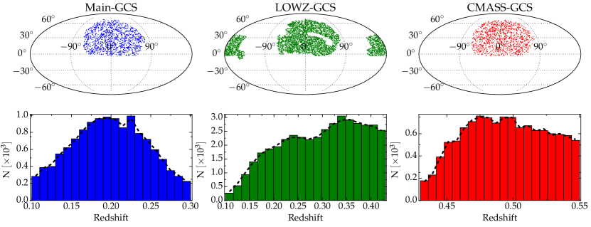
We restrict our redshift ranges to i) $0.1\leq z\leq 0.3$ for the Main-GCS, ii) $0.1\leq z\leq 0.43$ for the LOWZ-GCS, and iii) $0.43\leq z\leq 0.55$ for the CMASS-GCS. We have chosen the redshift cut at $z<0.43$ so that the CMASS-GCS and the LOWZ-GCS are independent samples. On the other hand, a significant fraction of clusters is in common between the Main-CGS and the LOWZ-CGS samples. We choose this sample splitting to maximize the number of clusters in each redshift bin and to simplify the creation of random catalogues. We discuss the covariance between samples in § 4. Table 1 reports the main properties of the selected samples, while in Fig. 1 we show their angular (upper panels) and redshift distributions (lower panels). The LOWZ-CGS results to be the largest cluster sample ever used in a clustering analysis, almost two times larger than the one used in Veropalumbo et al. (2014).

Figure 1: The angular (top panels) and redshift distributions (bottom panels) of the three selected galaxy cluster catalogues: Main-GCS (blue), LOWZ-GCS (green) and CMASS-GCS (red). The black dashed curves in the bottom panels are the reconstructed redshift distributions used for the construction of random catalogues.

Table 1: The main properties of the cluster samples used for the clustering analysis. The bias has been obtained by modelling the projected correlation function in the scale range $5<r[\,\mathrm{Mpc}\,h^{-1}\,]<20$ (see §3.1.3).

Sample Name	Number of clusters	Redshift Range	Median Redshift	bias
Main-GCS	$12910$	$0.1\leq z\leq 0.3$	$0.20$	$2.00\pm 0.05$
LOWZ-GCS	$42115$	$0.1\leq z\leq 0.43$	$0.30$	$2.42\pm 0.02$
CMASS-GCS	$11816$	$0.43\leq z\leq 0.55$	$0.50$	$3.05\pm 0.07$

2.3 Weights

We apply a weight to each cluster to correct for mass and redshift incompleteness (see WHL for further details). The cluster samples result to be $75\%$ complete for the minimum mass threshold, and up to $100\%$ complete for $M_{200}>2\times 10^{14}M_{\odot}$, at $z<0.42$. The detection rate drops below $z>0.42$; this explains the difference in density between LOWZ-GCS and CMASS-GCS. Moreover, for the CMASS-GCS sample, we take into account the dependence on seeing and stellar density of targets on the celestial sphere, as introduced in Anderson et al. (2012), to obtain a more consistent estimate of the 2PCF at large scales. This weighting scheme lowers the 2PCF normalization by $<10\%$. Thus, it can be considered as a minor effect considering the 2PCF uncertainites at the BAO scales.

3 Clustering measurements

In the following we describe all the steps concerning the estimate of the 2PCF from the samples described above, and the distance constraints obtained from the BAO fitting

3.1 The two-point correlation function

We measure the 2PCF using the Landy & Szalay (1993) estimator:

$$\xi(s)=\frac{DD(s)+RR(s)-2DR(s)}{RR(s)}\,,$$ (1)

where $DD(s)$, $RR(s)$ and $DR(s)$ are the data-data, random-random and data-random normalized pairs counts, respectively, for a separation bin $s\pm\mathrm{d}s/2$. We measure the 2PCF up to $200\,\mathrm{Mpc}\,h^{-1}\,$ in bins of $8\,\mathrm{Mpc}\,h^{-1}\,$, for the Main-GCS and the LOWZ-GCS, and in bins of $10\,\mathrm{Mpc}\,h^{-1}\,$ for the sparser CMASS-GCS sample.

3.1.1 Geometrical distortions

To estimate the comoving separations between object pairs, a fiducial cosmology has to be assumed. Indeed, the 3D 2PCF is not a cosmology-independent quantity, and when constraining the BAO peak we have to take into account the geometrical distortions introduced by a possible wrong assumption of the background cosmology.

As a fiducial cosmology, we assume a flat $\Lambda$ cold dark matter (CDM) model with Hubble constant $H_{0}=68\,\,\mathrm{km}\,\mathrm{s}^{-1}\mathrm{Mpc}^{-1}\,$, total matter density parameter $\Omega_{M}=0.3$, baryon density parameter $\Omega_{b}=0.045$, primordial spectral index $n_{s}=1$, and matter power spectrum normalization corresponding to $\sigma_{8}=0.83$.

3.1.2 Redshift-space distortions

The measured redshifts do not contain only distance information, being perturbed by the line-of-sight peculiar motions of the mass tracers. This introduces the so-called dynamical distortions in the clustering pattern. Specifically, both linear distortions, caused by ordered large-scale flows, and non-linear distortions, caused by random peculiar motions, are generally present. While linear distortions are always present, non-linear dynamical distortions have a very minor impact on BCGs, compared to satellite galaxies, since BCGs trace the bottom of the cluster potential wells. We verified this important aspect by looking at the two-dimensional 2PCF of galaxies and galaxy clusters. The former shows a very clear signal of the so-called Fingers of God, due to the random motions of satellites in haloes. On the other hand, this signal is almost absent in the 2PCF of galaxy clusters (Marulli et al., 2015). Photometric redshift errors can be fairly considered as a limiting case of peculiar motions. We then expect that non-linear distortions have limited effects on BCGs with spectroscopic redshift (see e.g. Marulli et al., 2015, and references therein). This reflects in a sharper BAO signal for this kind of tracers. We discussed how much these effects impact the galaxy cluster clustering in Veropalumbo et al. (2014).

3.1.3 Bias determination

To estimate the linear bias $b$ of our cluster samples, we use the projected correlation function defined as follows:

$$w_{p}(r_{p})=\int_{0}^{\pi_{max}}\mathrm{d}\pi^{\prime}\xi(r_{p},\pi^{\prime})\,,$$ (2)

where $\xi(r_{p},\pi)$ is the 2PCF measured in bins of perpendicular, $r_{p}$, and parallel, $\pi$, separations with respect to the line-of-sight. Integrating along the direction parallel to the line-of-sight allows us to approximately correct for redshift-space distortions. In Eq. 2 we set $\pi_{max}=50\,\mathrm{Mpc}\,h^{-1}\,$.

To obtain the bias, we model the projected correlation functions as follows:

$$w_{p}(r_{p})=b^{2}\int_{r_{p}^{2}}^{\sqrt{\pi_{max}^{2}+r_{p}^{2}}}\mathrm{d}r\frac{2r\xi(r)}{\sqrt{r^{2}-r_{p}^{2}}},$$ (3)

where $\xi(r)$ is the predicted matter power spectrum. This measure allows us to construct a cluster 2PCF model, to be used in the covariance matrix estimate via lognormal mock catalogues (see § 3.3.2).

3.2 Random catalogues

According to Eq. 1, a random sample has be provided to correctly evaluate the 2PCF. A random catalogue contains the information on the selection function of the data sample, that are used to balance spurious effects affecting the pair counting. The selection function can be safely reproduced separating it into angular and radial parts. We generate random catalogues almost 20 times larger than the reference cluster samples to limit shot noise effects.

3.2.1 Angular mask

We generate random points using publicly available survey footprints and the MANGLE software (Swanson et al., 2008). For the three cluster samples we used the following masks:

• Main-GCS: the SDSS DR7 survey footprint, using the window provided by the NYU-VAGC (Blanton et al., 2005);

• Lowz-GCS: the BOSS survey footprint, excluding regions with bugged target selections (IPOLY $>10324$);

• CMASS-GCS: the Northern Galactic Cap of BOSS survey footprint.

We mask random points falling in the veto regions, as done for the data.

3.2.2 Cluster redshift distribution

We consider two methods to assign redshifts to the random collections of objects:

• random extraction from the smoothed redshift distribution; the parameters involved are the redshift bin and the size of the Gaussian kernel;

• random assigning from the galaxy cluster redshifts (see Ross et al., 2012).

We verified that all our results are robust independently of the method and adopted parameters. In the following, we will show results obtained with the first method, grouping the cluster redshift distribution in $100$ bins and smoothing the redshift distribution with a Gaussian kernel three times larger than the bin size.

3.3 Covariance matrix

The covariance matrix is a crucial ingredient for clustering analyses. It measures the correlation between correlation function bins, and it is defined as follows:

$$C_{i,j}=\frac{1}{N-1}\sum_{k=1}^{N}(\xi^{k}_{i}-\hat{\xi_{i}})(\xi^{k}_{j}-\hat{\xi_{j}})\,,$$ (4)

where the subscripts $i$ and $j$ run over spatial bins of the correlation function and $k$ refers to the 2PCF of the $k^{th}$ of $N$ realizations; $\hat{\xi}$ is the mean 2PCF of the $N$ realizations.

The covariance matrix can be directly estimated using mock catalogues extracted from numerical simulations (see e.g. Anderson et al., 2014; Kazin et al., 2014). However, this method is very computational expensive if a large set of mocks have to be created. Alternatively, different statistical techniques can be exploited, that still provide fairly robust estimates of the covariance matrix. For our analysis, we consider the following approaches to estimate the covariance matrix:

• two internal error estimators: jackknife and bootstrap (see e.g. Norberg et al., 2009);

• one external error estimator, that exploits lognormal mocks generated from the density field.

3.3.1 Internal errors

The covariance matrix can be estimated by subsampling the original catalogue and calculating the correlation function in all but one sub- samples (jackknife), or in a random selection of them (bootstrap), recursively. We choose to subsample the observations in $50$ right ascension-declination regions, that results in $50$ jackknife mock realizations, while we extract $200$ times these subregions to exploit the bootstrap resampling.

3.3.2 External errors

We compare the internal error estimates described above with the ones assessed through the lognormal density field technique (Coles & Jones, 1991). This method to infer the covariance matrix has been already used by several authors for clustering analyses (see e.g. Beutler et al., 2011; Blake et al., 2011; Chuang et al., 2014).

We create the density field realizations using the redshift-space monopole model:

$$P_{model}(k)=b^{2}\left(1+\frac{2}{3}\beta+\frac{1}{5}\beta^{2}\right)P_{DM}(k)\,,$$ (5)

where $P_{DM}$ is the linear matter power spectrum obtained with the CAMB software (Lewis & Bridle, 2002), $b$ is the bias constrained from the galaxy cluster projected correlation function at the small scales, and $\beta$ is the ratio between the linear growth rate function $f=\Omega_{M}(z)^{0.545}$, as predicted by General Relativity, and the bias $b$. To measure $b$ we model the projected correlation function as described in §3.1.3. The covariance matrix used for the fit is the one derived with the sub-sampling approach. The estimated values of the bias and its standard deviation for each sample are reported in Table 1.

Density fields are generated in boxes large enough to contain the survey volumes, with a regular grid of steps half the size of the bins used to estimate the 2PCF. The survey selection function is taken into account in the random catalogues. Once the mock clusters are extracted according to the density distribution, the covariance matrix can be directly estimated by measuring the 2PCF for each mock sample.

3.4 Model

In this section we describe the models used to derive distance constraints from the BAO peak in the 2PCF.

3.4.1 Fitting the 2PCF

To extract cosmological constraints from the BAO peak, we adopt the following widely used and robust model (see Anderson et al., 2012, and reference therein):

$$\xi(r)\,=\,B^{2}\xi_{DM}(\alpha r)+A_{0}+\frac{A_{1}}{r}+\frac{A_{2}}{r^{2}}\,,$$ (6)

where $\xi_{DM}(r)$ is the dark matter 2PCF calculated assuming the fiducial cosmology, $B$ factorises the difference between the dark matter 2PCF and the cluster 2PCF, $\alpha$ is the parameter that contains the distance information, and $A_{0}$, $A_{1}$ and $A_{2}$ are the parameters of an additive polynomial used to marginalize over signals caused by systematics not fully taken into account.

We adopt the de-wiggled template for the dark matter power spectrum, $P_{DM}$ (Eisenstein, Seo & White, 2007):

$$P_{DM}(k)\,=\,\left[P_{lin}(k)-P_{nw}(k)\right]\mathrm{e}^{-k^{2}\Sigma_{NL}^{2}/2}+P_{nw}(k)\,,$$ (7)

where $P_{lin}$ is the linear power spectrum as provided by CAMB (Lewis & Bridle, 2002), while $P_{nw}$ is the power spectrum without the BAO feature, as obtained by the parametric formula of Eisenstein & Hu (1998). The parameter $\Sigma_{NL}$ controls the smearing of the BAO, and it is left free to vary. The model for $\xi_{DM}(r)$ is then obtained by Fourier transforming the power spectrum:

$$\xi_{DM}(r)=\frac{1}{2\pi^{2}}\int\mathrm{d}k\,k^{2}P_{DM}(k)\frac{\sin(kr)}{kr}\,.$$ (8)

To get marginalized constraints we populate the parameter space with the Monte Carlo Markov Chain technique. We adopt a Gaussian likelihood, $\propto\exp(-\chi^{2}/2)$, with $\chi^{2}$ defined as follows:

$$\chi^{2}=\sum_{i=0}^{n}\sum_{j=0}^{n}(\xi_{i}-\xi^{m}(r_{i}))C^{-1}_{ij}(\xi_{j}-\xi^{m}_{j})\,,$$ (9)

where $\xi_{i}$ is the 2PCF measured in the $i^{th}$ bin, $\xi^{m}_{i}$ is the model in the same bin and $C^{-1}_{ij}$ is the inverted covariance matrix.

Figure 2: The redshift-space 2PCF of galaxy clusters, respectively Main-GCS (left panel), LOWZ-CGS (central panel) and CMASS-CGS (right panel). The errorbars are computed with the lognormal mock method. The dashed line shows the best-fit model from Eq. 6. The shaded area represents the $68\%$ posterior uncertainties provided by the MCMC analysis.

3.4.2 The BAO distance constraint

The distance constraint is entirely contained in $\alpha$ (Eq. 6). Correcting for the geometric distortions, it can be derived through the following approximation:

$$D_{V}(\bar{z})\,=\,\alpha D_{V}^{fid}(\bar{z})\left(\frac{r_{s}}{r_{s}^{fid}}\right)\,\mathrm{Mpc}\,\,.$$ (10)

Eq. 10 states that the distance constrained at the mean redshift of the catalogue is $\alpha$ times the distance at the fiducial cosmology, scaled to the ratio between the true and fiducial sound horizon. $D_{V}(\bar{z})$ is the isotropic volume distance calculated at the mean redshift of the catalogue:

$$D_{V}(z)\,=\,\left[(1+z)^{2}D_{A}^{2}(z)\frac{cz}{H(z)}\right]^{1/3}\,,$$ (11)

where $c$ is the speed of light, $D_{A}(z)$ is the angular diameter distance and $H(z)$ is the Hubble parameter at redshift $z$. If we assume that the true value of the sound horizon is known, we can directly measure a distance; otherwise we can exploit only an uncalibrated version of the standard ruler technique, measuring the ratio $D_{V}(z)/r_{s}$. In the following, cosmological constraints will be obtained using both the calibrated and the uncalibrated distance estimators.

4 Results

4.1 Sample covariance

Firstly, we test the covariance in the parameter estimation among the two catalogues with data in common, the Main-GCS and the Lowz-GCS. We construct $100$ lognormal realizations extracting samples according to the sample selection function. Then we add the same fraction of data in common between the samples (almost $2/3$ of the Main-GCS). After measuring the 2PCF for each realization, we fitted a simple two-parameter model for the $\xi(r)$:

$$\xi(r)=b^{2}\xi_{DM}(\alpha r)\,,$$ (12)

where $b$ is the bias factor and $\alpha$ is the shift parameter. We then calculate the correlation index $\rho$ as the ratio $C_{ij}/\sqrt{C_{ii}*C_{jj}}$ with $C_{ij}=<\alpha_{i}\alpha_{j}>-<\alpha_{i}><\alpha_{j}>$. We find a moderate correlation, with $\rho=0.402$.

4.2 Clustering measurements

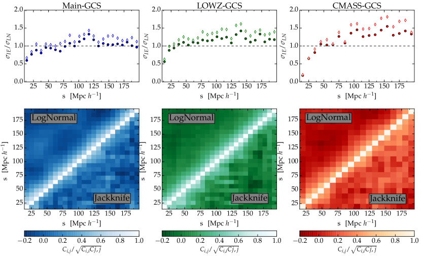
In Fig. 2 we present the measured 2PCF for the three galaxy cluster samples considered. The errorbars shown are the ones computed with the lognormal mock method. Measures are robust when changing the modelization of the radial selection function. The clustering signal is well determined despite the sparseness of the samples. The measured 2PCFs are all consistent with each other in terms of the BAO peak position, though a significant difference in the bias is measured (see Table 1). As already pointed out in § 3.3, we consider different methods to compute the covariance matrix. In the case of internal errors, we divide each cluster catalogue in $100$ samples to get the jackknife estimate, and re-sample them $200$ times to exploit the bootstrap technique. We use instead $1000$ lognormal mock realizations. Results are shown in Fig. 3. In the top panels we compare internal estimates (filled circles for jackknife, open diamonds for bootstrap) and lognormal mock estimates of the square root of the principal diagonal values of the covariance matrix. Internal methods provide conservative estimates of the errors, that become less biased for larger number of objects. Both the jackknife and bootstrap estimates are robust when changing the number of subsamples, or resamplings. Nevertheless, a large number of realizations makes the covariance matrix less scattered. This can be seen in the bottom panels of Fig. 3: the covariance matrix obtained with lognormal mocks is smoother compared to the jackknife one. In the following we adopt the lognormal mock estimate of the covariance matrix as the reference. Covariance matrices from internal estimators will be used to check for consistencies in the parameter determination and BAO peak detection.

Figure 3: Upper panels: ratio of internal error (jackknife: filled circles, bootstrap: open diamonds) and lognormal principal diagonal square roots. At the scales of interest for the fit, internal error methods provide a conservative error estimate. Lower panels: correlation matrices ($C_{i,j}/\sqrt{C_{i,i}C_{j,j}}$) from lognormal realizations (upper diagonal part) and from jackknife estimates (lower diagonal part). The $1000$ lognormal mocks provide a less scattered covariance matrix with respect to the jackknife method. This is due mainly to the low number of bins ($50$) used when resampling the catalogue.

Figure 4: The values of $\Delta\chi^{2}$ as a function of $\Sigma_{NL}$ for the three cluster samples – Main-GCS (left panel), LOWZ-GCS (centeral panel), and CMASS-GCS (right panel) – and for the three covariance matrix definitions – lognormal mocks (blue filled circles), jackknife (red squares) and bootstrap (yellow diamonds). The values span from a linear power spectrum ($\Sigma_{NL}\,=0\,\,\mathrm{Mpc}\,h^{-1}\,$) to a power spectrum model with no BAO ($\Sigma_{NL}\,\rightarrow\infty$). Detections of the BAO are well over $2\sigma$ in all cases.

Table 2: Values of the shift parameter $\alpha$ for the three catalogues, obtained using covariance matrices from lognormal mocks, jackknife and bootstrap subsampling, from column $2$ to column $4$. All the results have been obtained by fitting the 2PCF from $40\,\mathrm{Mpc}\,h^{-1}\,$ to $200\,\mathrm{Mpc}\,h^{-1}\,$, and fixing $\Sigma_{NL}=4\,\mathrm{Mpc}\,h^{-1}\,$.

Sample Name	LogNormal	Jackknife	Bootstrap
Main-GCS	$0.97\pm 0.06$	$0.97\pm 0.08$	$0.98\pm 0.08$
LOWZ-GCS	$0.99\pm 0.03$	$0.99\pm 0.04$	$0.99\pm 0.05$
CMASS-GCS	$0.99\pm 0.03$	$0.99\pm 0.06$	$0.99\pm 0.08$

4.3 Distance constraints

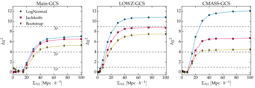
We get distance constraints by fitting the BAO peak position in the measured 2PCF at different redshifts. The BAO feature is clearly detected for all samples. Results of the fits using the different definitions of the covariance matrix are reported in Table 2. The $\alpha$ values estimated in the three redshift bins are all consistent. The precision in the detection degrades when using jackknife or bootstrap covariance matrices, as expected. The model depends on the parameter $\Sigma_{NL}$, that describes the degradation of the BAO feature in the power spectrum. We fit the measured 2PCF by changing this parameter from $0$ to $100\,\mathrm{Mpc}\,h^{-1}\,$. Fig. 4 shows the values of $\Delta\chi^{2}$ as a function of $\Sigma_{NL}$. Each point represents the difference between the minimum $\chi^{2}$ at each $\Sigma_{NL}$ and the absolute minimum of the curve. We do this for all the three samples and for the three error definitions. This allows us to determine the significance of our detection. Indeed, for high values of $\Sigma_{NL}$, the BAO peak completely disappears ($\xi(r)\rightarrow\xi_{nw}$, see Eq. 7). The significance of the BAO detections result to be well above $2\sigma$ for all the considered samples. We cannot distinguish between models with $\Sigma_{NL}<8\,\mathrm{Mpc}\,h^{-1}\,$, that are all consistent within $1\sigma$. Nevertheless, Fig. 4 clearly indicates that galaxy clusters have a more limited non-linear contribution at the BAO scales with respect of other tracers, such as galaxies (the $\Delta\chi^{2}$ minima are in some cases at $\Sigma_{NL}=0\,\mathrm{Mpc}\,h^{-1}\,$). This result confirms what found in Veropalumbo et al. (2014). A practical consequence is that the density field reconstruction seems not crucial in the BAO distance constraints from galaxy clusters. We will return to this aspect in § 4.5, while a more detailed investigation is postponed to a forthcoming work. Hereafter we consider the lognormal results with $\Sigma_{NL}=4\,\mathrm{Mpc}\,h^{-1}\,$ as our reference distance constraint.

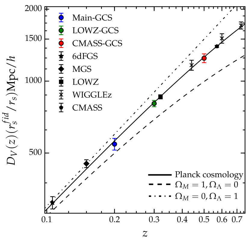
We measure the following values: $D_{V}(z=0.2)(r_{s}^{fid}/r_{s})=545\pm 31\,\mathrm{Mpc}\,h^{-1}\,$, $D_{V}(z=0.3)(r_{s}^{fid}/r_{s})=806\pm 24\,\mathrm{Mpc}\,h^{-1}\,$ and $D_{V}(z=0.5)(r_{s}^{fid}/r_{s})=1247\pm 53\,\mathrm{Mpc}\,h^{-1}\,$. Fig. 5 shows the distance-redshift diagram. The coloured points are the isotropic distance estimates for the Main-GCS (blue), the LOWZ-GCS (green) and the CMASS-GCS (red) sample, respectively. The other black symbols show some $D_{V}$ estimates for galaxy samples from literature: 6dFGS survey (Beutler et al., 2011, black star), Main galaxy sample (MGS) from SDSS DR7 (Ross et al., 2015, black diamond), BOSS LOWZ and CMASS (Anderson et al., 2014, black square and pentagon, respectively) and WiggleZ (Kazin et al., 2014, black cross). The black curve is the theoretical prediction for the Planck 2013 $\Lambda$CDM cosmology (Planck Collaboration et al., 2014). As it can be seen, our results are fully consistent with previous measurements from galaxy surveys, and with standard $\Lambda$CDM predictions.

4.4 Cosmological implications

We can use the distance measurements described above to derive constraints on cosmological parameters. Using only the three measures obtained with our cluster samples we do not expect to get constraints competitive with the ones obtained by combining larger galaxy samples with different probes. The aim here is just to check the consistency of our measurements with the predictions of the standard cosmological framework.

As reported in § 3.4.2, we consider two methods to derive cosmological constraints, that is the calibrated and the uncalibrated distance estimators. In the first case, we use the Planck value of the sound horizon, $r_{s}=147.34\pm 0.65\,\mathrm{Mpc}\,$, to calibrate the BAO distance measure. We have $D_{v}(z=0.2)=800\pm 50\,\mathrm{Mpc}\,$, $D_{V}(z=0.3)=1183\pm 35\,\mathrm{Mpc}\,$ and $D_{V}(z=0.5)=1832\pm 55\,\mathrm{Mpc}\,$. In the second approach the sound horizon is a function of cosmological parameters, through the interpolation formula given by Anderson et al. (2014). In this case we get $r_{s}/D_{V}(z=0.2)=0.18\pm 0.01$, $r_{s}/D_{V}(z=0.3)=0.124\pm 0.004$ and $r_{s}/D_{V}(z=0.5)=0.080\pm 0.002$. The value of $\Omega_{b}$ is kept fixed to the best-fit Planck value (Planck Collaboration et al., 2014): $\Omega_{b}=0.049$.

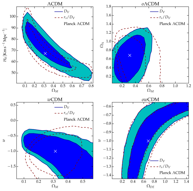
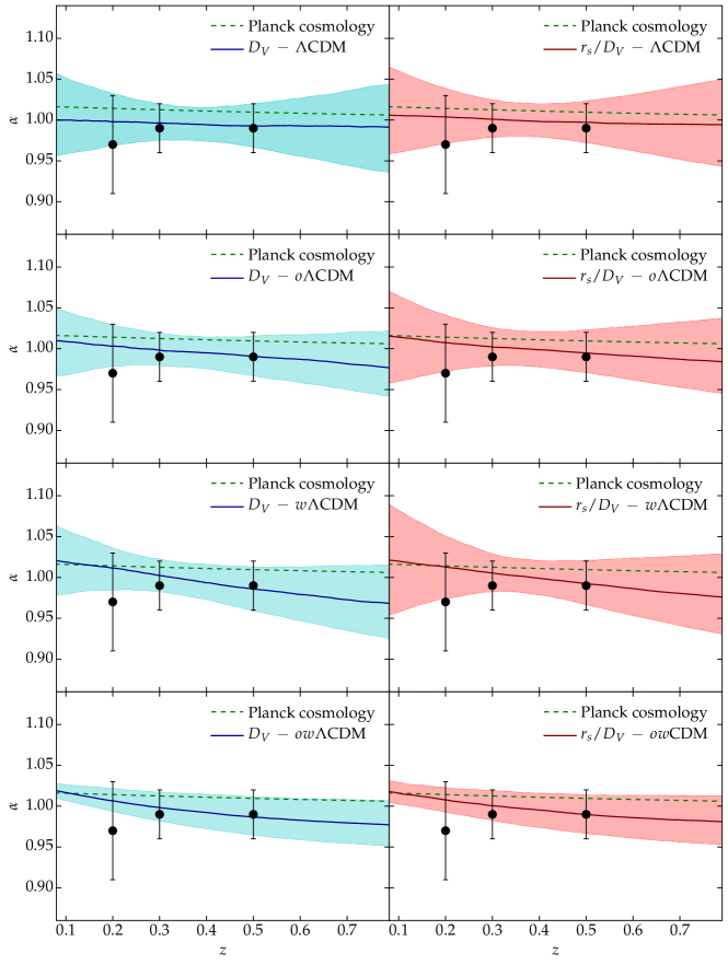
With both the methods we test some cosmological scenarios. Specifically, we constrain the cosmological parameters that enter the Hubble function, $H(z)$. In fact, the quantity $D_{V}$ is a function of $H(z)$ and of the angular diameter distance $D_{A}(z)$, which in turn depends on the comoving distance $D_{C}(z)=\int_{0}^{z}\mathrm{d}z^{\prime}c/H(z^{\prime})$ (Eq. 11). Results of all the fits are summarized in Table 3, Fig. 6, where we show constraints of cosmological parameters and in Fig. 7, where we show the best-fit values of $\alpha$ (Eq. 10) for the two types of distances and for four different cosmological scenarios.

4.4.1 $\Lambda$CDM models

The simplest model we test is the flat $\Lambda$CDM Universe (equation of state $w=-1$), with a negligible contribution of radiation. In this case the Hubble function reads:

$$H^{2}(z)/H^{2}_{0}=\Omega_{M}(1+z)^{3}+\Omega_{\Lambda}.$$ (13)

Since the curvature $\Omega_{k}=1-\Omega_{M}-\Omega_{\Lambda}-\Omega_{r}$ is fixed to zero, $\Omega_{\Lambda}$ is a function of $\Omega_{M}$. We fit our distance constraints against the pair $\{\Omega_{M},H_{0}\}$. We impose a large uniform prior on both parameters: $\mathcal{U}(0,1)$ for $\Omega_{M}$ and $\mathcal{U}(30,120)$ for $H_{0}$. Here $\mathcal{U}(a,b)$ is the uniform distribution, equal to $0$ outside ranges $a,b$. We find $\Omega_{M}=0.32^{+0.21}_{-0.14}$ and $H_{0}=72^{+13}_{-13}\,\,\mathrm{km}\,\mathrm{s}^{-1}\mathrm{Mpc}^{-1}\,$ for the calibrated distance indicator, and $\Omega_{M}=0.32^{+0.22}_{-0.15}$ and $H_{0}=64^{+17}_{-9}\,\,\mathrm{km}\,\mathrm{s}^{-1}\mathrm{Mpc}^{-1}\,$ for the uncalibrated case. Results are summarized in Fig. 6 (upper left panel), where we show the $1-2\sigma$ confidence contours for the parameters $\Omega_{M}-H_{0}$, and in the upper row in Fig. 7. The Planck cosmology is well compatible with our results, in both cases. Our constraints are broad, due to our distance uncertainties and to our limits in redshift. As we will show in particular for the next cases, high-redshift distance measures significantly help in measuring the geometry of the Universe.

Figure 5: The distance $D_{V}(z)/(r_{s}^{fid}/r_{s})$ – redshift relation. The coloured points show our measurements at redshifts $0.2,0.3,0.5$. Other black symbols correspond to other distance constraints from galaxy surveys: 6dFGS (Beutler et al., 2011, star), MGS (Ross et al., 2015, diamond) , BOSS LOWZ and CMASS (Anderson et al., 2014, square and pentagon, respectively) and WiggleZ (Kazin et al., 2014, crosses). The black curve is the $D_{V}(z)$ prediction for the $\Lambda$CDM cosmology with the Planck parameters (Planck Collaboration et al., 2014). We also show distance prediction in a flat, matter-only Einstein-De Sitter universe (black dashed curve) and for a De Sitter universe with $\Omega_{\Lambda}=1$ (black dot-dashed curve)

Figure 6: $1-2\sigma$ confidence contours for parameters assuming different cosmological models: $\Omega_{M}$-$H_{0}$ plane in the $\Lambda$CDM model (upper left panel), $\Omega_{M}-\Omega_{\Lambda}$ plane in the $o\Lambda$CDM model (upper right panel), $\Omega_{M}-w$ plane in the $w$CDM model (lower left panel) and $\Omega_{DE}-w$ plane in the $ow$CDM model(lower right panel). The red dashed contours show results from the uncalibrated distance $r_{s}/D_{V}$, the blue for the calibrated distance $D_{V}$. The best fit value for Planck $\Lambda$CDM cosmology is also reported (black cross).

Figure 7: The best-fit values of $\alpha(z)\equiv D_{V}(z)/r_{s}/(D_{V}(z)/r_{s})^{fid}$ (solid curves) and $68\%$ model error (shaded areas) using the calibrated and uncalibrated BAO distances (black dots, respectively in the left and right panels). We show results for the four cosmological model tested: $\Lambda$CDM (first row), $o\Lambda$CDM (second row), $w$CDM (third row) and $ow$CDM (fourth row). The Planck best-fit values for $\alpha$ are shown by the green dashed curves. For the fit with calibrated distances, we assumed the Planck value for the sound horizon.

4.4.2 $o\Lambda$CDM models

Here we test our measurements against a non-flat Universe with CDM and cosmological constant. In this case the Hubble equation becomes:

$$H^{2}(z)/H^{2}_{0}=\Omega_{M}(1+z)^{3}+\Omega_{\Lambda}+\Omega_{k}(1+z)^{2}.$$ (14)

We fit the combination of parameters $\{\Omega_{M},\Omega_{\Lambda},H_{0}\}$, using a flat prior on $\Omega_{M}$, $\Omega_{\Lambda}$ and a broad Gaussian prior on $H_{0}$ $\mathcal{N}(\mu,\sigma)$ with mean $\mu$ centered on the Planck value $67\,\mathrm{km}\,\mathrm{s}^{-1}\mathrm{Mpc}^{-1}\,$, and standard deviation $\sigma$ of $20\,\mathrm{km}\,\mathrm{s}^{-1}\mathrm{Mpc}^{-1}\,$. See Tab. 3 for more information on the adopted priors. We find $\Omega_{k}=0.05\pm 0.40$ for the $D_{V}$ fit and $\Omega_{k}=-0.01_{-0.36}^{+0.34}$ for the fit using $r_{s}/D_{V}$. In Fig. 6 (upper right panel) we show the $1-2\sigma$ confidence contours for the combination $\Omega_{M}-\Omega_{\Lambda}$, marginalized over $H_{0}$. We confirm at $1\sigma$ the necessity of a negative pressure component in the cosmological model. The different degeneracy directions obtained with the two methods are due to the introduction of the cosmological dependence of the sound horizon, that depends only on $\Omega_{M}h^{2}$ and $\Omega_{b}h^{2}$. In Fig. 7, second row, we can appreciate the increasing difference between the Planck $\Lambda$CDM best-fit model (dashed green curve) and the best-fit model obtained with our data (blue solid line), going to high redshifts. The difference is well inside $1\sigma$, due to our distance uncertainties, though a little tension with the Planck results can be noticed.

Table 3: Summary of the cosmological parameters obtained by fitting the calibrated BAO distance $D_{V}$ and the uncalibrated BAO distance $d_{z}$. We report priors used in the fitting procedures.

	Distance	$H_{0}[\,\mathrm{km}\,\mathrm{s}^{-1}\mathrm{Mpc}^{-1}\,]$		$\Omega_{M}$		$\Omega_{\Lambda}/\Omega_{DE}$		$w$
		Prior	Posterior	Prior	Posterior	Prior	Posterior	Prior	Posterior
$\Lambda$CDM	$D_{V}$	$\mathcal{U}(30,120)$	$72^{+13}_{-13}$	$\mathcal{U}(0,1)$	$0.32^{+0.21}_{-0.14}$	$-$	$-$	$-$	$-$
	$d_{z}$	$"$	$64^{+17}_{-9}$	$"$	$0.32^{+0.22}_{-0.15}$	$-$	$-$	$-$	$-$
$o\Lambda$CDM	$D_{V}$	$\mathcal{N}(67,20)$	$70^{+11}_{-10}$	$\mathcal{U}(0,1)$	$0.32^{+0.15}_{-0.14}$	$\mathcal{U}(0,1.5)$	$0.63^{+0.30}_{-0.29}$	$-$	$-$
	$d_{z}$	$"$	$62^{+14}_{-12}$	$"$	$0.36^{+0.19}_{-0.13}$	$"$	$0.65^{+0.33}_{-0.37}$	$-$	$-$
$w$CDM	$D_{V}$	$\mathcal{N}(67,20)$	$69^{+11}_{-10}$	$\mathcal{U}(0,1)$	$0.39^{+0.16}_{-0.18}$	$-$	$-$	$\mathcal{U}(-2,0)$	$-1.15^{+0.43}_{-0.54}$
	$d_{z}$	$"$	$64^{+12}_{-8}$	$"$	$0.38^{+0.19}_{-0.12}$	$-$	$-$	$"$	$-1.01^{+0.44}_{-0.44}$
$ow$CDM	$D_{V}$	$\mathcal{N}(67,2)$	$67.0^{+1.4}_{-1.4}$	$\mathcal{N}(0.31,0.02)$	$0.31^{+0.01}_{-0.01}$	$\mathcal{U}(0,1.5)$	$0.66^{+0.45}_{-0.24}$	$\mathcal{U}(-1.5,0)$	$-0.91^{+0.23}_{-0.38}$
	$d_{z}$	$"$	$67.0^{+1.4}_{-1.4}$	$"$	$0.31^{+0.01}_{-0.01}$	$"$	$0.66^{+0.46}_{-0.21}$	$"$	$-0.88^{+0.24}_{-0.36}$

4.4.3 $w$CDM models

We now test our data against a flat Universe with CDM and dark energy, with dark energy density changing with time. We parametrize the dark energy density time dependence with a constant $w$ equation of state. The Hubble equation in this case is:

$$H^{2}(z)/H^{2}_{0}=\Omega_{M}(1+z)^{3}+\Omega_{DE}(1+z)^{3(1+w)}.$$ (15)

This model turns into standard $\Lambda$CDM cosmology imposing $w=-1$. We fit the combination of parameters $\{\Omega_{M},w,H_{0}\}$, since, as in the $\Lambda$CDM case, the value of $\Omega_{DE}$ at the present time is fixed by the relation $\Omega_{DE}=1-\Omega_{M}$. We assume a flat prior on $\Omega_{M}$ and $w$ and a broad Gaussian prior on $H_{0}$, centered at the Planck value $67\,\mathrm{km}\,\mathrm{s}^{-1}\mathrm{Mpc}^{-1}\,$, with standard deviation of $20\,\mathrm{km}\,\mathrm{s}^{-1}\mathrm{Mpc}^{-1}\,$. We find $w=-1.15_{-0.54}^{+0.43}$ for the calibrated distance fit, and $w=-1.01_{-0.44}^{+0.44}$ for the uncalibrated one. Confidence contours up to $2\sigma$ for the pair $\Omega_{M}-w$ are shown in Fig. 6 (lower left panel), while the best-fit corresponding value of $\alpha$ is reported in the third row of Fig. 6.

4.4.4 $ow$CDM models

The most general case we consider is the one with a non-flat Universe with time-dependent dark energy density:

$$H^{2}(z)/H^{2}_{0}=\Omega_{M}(1+z)^{3}+\Omega_{DE}(1+z)^{3(1+w)}+\Omega_{k}(1+z)^{2}.$$ (16)

We vary the parameters $\{\Omega_{M},\Omega_{DE},w,H_{0}\}$, keeping totally free $\Omega_{DE}$ and $w$, and assuming a Gaussian prior for $\Omega_{M}$, centered on $0.31$ with a standard deviation of $0.02$, and for $H_{0}$ centered on $67\,\mathrm{km}\,\mathrm{s}^{-1}\mathrm{Mpc}^{-1}\,$ with a small standard deviation of $2\,\mathrm{km}\,\mathrm{s}^{-1}\mathrm{Mpc}^{-1}\,$, respectively. In the case of the uncalibrated distance measure, the strong priors on $\Omega_{M}$ and $H_{0}$ resume in an almost constant value for the sound horizon. Since the central values for these two parameters are the ones from Planck, the value of the sound horizon is centered on the Planck value too. This explains the similarity in the bottom row of Fig. 7, comparing the calibrated and uncalibrated version of the fit. Fig. 6 (lower right panel) shows the degeneracy between the parameters $\Omega_{DE}$ and $w$. Even with the assumption of these strong priors, no clear constraint can be extracted in this case. In Table 3 we report the $16-84th$ percentile interval of the parameter posterior distribution.

4.5 Comparison with previous measurements

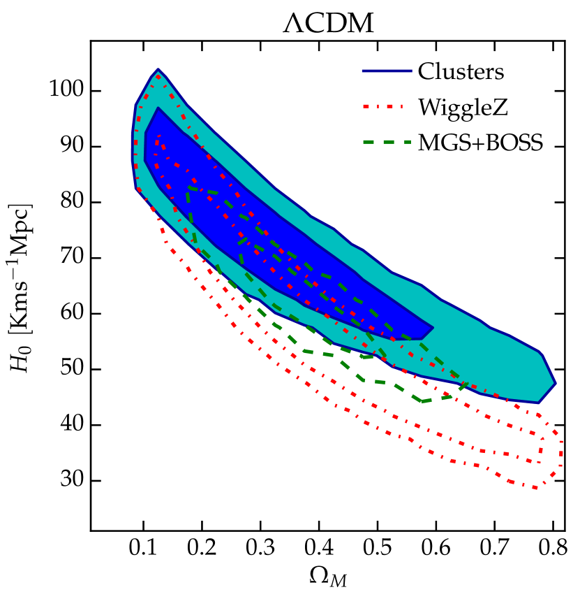
Fig. 8 shows the posterior $1-2\sigma$ confidence contours of $\Omega_{M}$–$H_{0}$ parameters, obtained with the calibrated distance estimators (see § 3.4.2) from the BAO of the galaxy cluster samples considered in this work, and of the galaxy samples of MGS+BOSS and WiggleZ. As one can see, our constraints are consistent with previous estimates. Our uncertainties appear slightly better than the ones obtained by modelling the post-reconstruction WiggleZ clustering (Kazin et al., 2014), despite the paucity of our samples, while they are broader with respect to the ones from the BOSS survey. This is expected, since our BCGs represent a subsample of the BOSS galaxy survey. Indeed, the measurements obtained with these BOSS galaxy catalogues provide the best BAO distance constraints to date, both in term of accuracy and of BAO reconstruction and modelling techniques.

Compared to clusters, we find a lower value of the bias factor for the BOSS galaxies. This result is expected and implies that our cluster catalogues cannot be simply considered as random subsamples of the galaxy catalogue, but they identify the highest peaks of the density field, confirming our previous results (Veropalumbo et al., 2014).

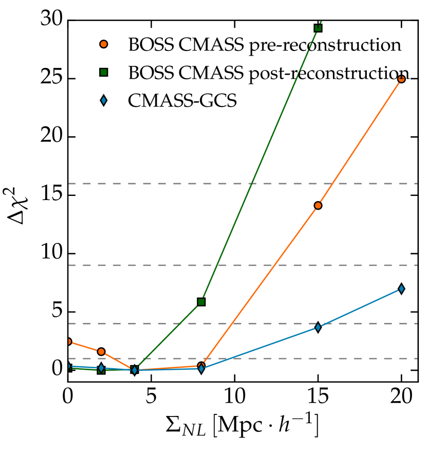
Finally, we reanalyze the BOSS CMASS clustering data with the method described in § 4.3. Fig. 9 shows the values of $\Delta\chi^{2}$ as a function of $\Sigma_{NL}$ for the BOSS CMASS pre- and post-reconstruction samples, and for our CMASS-GCS sample. Firstly, our estimated value of the BAO detection significance for the BOSS CMASS data is consistent with the value claimed by Anderson et al. (2014). Moreover, this analysis highlights the impact of the density field reconstruction technique, that shifts the best-fit value of $\Sigma_{NL}$ from $8\,\mathrm{Mpc}\,h^{-1}\,$ to $4\,\mathrm{Mpc}\,h^{-1}\,$ and lower, improving BAO distance constraints. On the other hand, galaxy clusters trace a more linear density field with respect to galaxies. Thus, we expect that the BAO constraints would not improve significantly as a result of the reconstruction technique, though we cannot draw any robust conclusion about this aspect due to our measure uncertainties.

5 Conclusions

In this work we obtained the first observational constraints on the distance-redshift relation using only the clustering properties of galaxy clusters. Specifically, we measured the 2PCF of the largest spectroscopic galaxy cluster samples to date, in three redshift ranges, and extract consmological constraints from the position of the BAO peak. The catalogues have been constructed by matching the BCGs from the WHL catalogue (Wen, Han & Liu, 2012), with spectra from SDSS DR7 (Abazajian et al., 2009) and SDSS DR12 (Alam et al., 2015). This allowed us to construct three catalogues of galaxy clusters – Main-GCS, LOWZ-GCS and CMASS-GCS – at the median redshift $z=0.2$, $0.3$ and $0.5$, respectively. We estimated the covariance matrix using both internal error estimators (jackknife and bootstrap) and with the lognormal mock method. These estimators provide fairly consistent errors, with internal errors more conservative and scattered. We choose the lognormal mock covariance matrix estimate as reference. The BAO feature is detected with a significance larger than $2\sigma$, for all considered samples. The derived cosmological constraints are competitive with respect to other estimates from the BAO peak obtained using richer galaxy catalogues, such as 6dFGS (Beutler et al., 2011) and WiggleZ (Blake et al., 2011). As expected, our results are instead not comparable in precision with the constraints coming from the BOSS survey, of which our BCGs represent a subsample. For the three samples analysed we get: $\alpha(z=0.2)=0.96\pm 0.06$, $\alpha(z=0.3)=0.99\pm 0.03$ and $\alpha(z=0.5)=0.99\pm 0.03$, respectively. This translates to the uncalibrated distance estimates: $r_{s}/D_{V}(z=0.2)=0.18\pm 0.01$, $r_{s}/D_{V}(z=0.3)=0.124\pm 0.004$, $r_{s}/D_{V}(z=0.5)=0.080\pm 0.002$. We use the sound horizon estimate from Planck Collaboration et al. (2014) to calibrate the distances, obtaining: $D_{V}(z=0.2)=800\pm 50\,\mathrm{Mpc}\,$, $D_{V}(z=0.3)=1183\pm 35$, $D_{V}(z=0.5)=1832\pm 55$. We then use both the uncalibrated and calibrated distance estimates to derive cosmological constraints. Our results are all consistent with the cosmological model supported by the Planck results (see Planck Collaboration et al., 2014). To disentangle cosmological parameter degeneracies we would need higher redshift-distance constraints.

Figure 8: Comparison of the $1-2\sigma$ confidence contours in the $\Omega_{M}-H_{0}$ plane between our work (blue filled contours) and previous measurements from galaxy samples – WiggleZ (red dot-dashed contours) and MGS+BOSS (green dashed contours).

Figure 9: The same as Fig. 4 but for BOSS CMASS before (orange filled circles) and after reconstruction (green filled squares) (Anderson et al., 2014) and CMASS-GCS, with lognormal mock covariance matrix (blue filled diamonds). The high significance of the BAO detection is evident for galaxies, compared to our results. The reconstruction process helps in reducing non-linear effects, shifting the $\Delta\chi^{2}$ minimum to $4\,\mathrm{Mpc}\,h^{-1}\,$ in the post-reconstruction measurement.

This study clearly demonstrates that galaxy clusters are powerful tracers of the cosmic density field and can be efficiently exploited for BAO analyses. Despite the paucity of cluster samples, with respect to generally larger galaxy samples, the higher values of cluster bias and the fact that their redshifts are less distorted by random motions improve the clustering signal, that results almost insensitive to non-linear dynamical distortions. This reflects in a sharper BAO peak in the 2PCF, close to the prediction of linear theory. To further tighten the cosmological constraints obtained in this work, we plan to combine these clustering measurements with estimates of the cluster mass function. These investigations will be presented in a forthcoming paper. The techniques presented here will be further exploited in the next future on the increasingly large collections of data expected from new experiments like e.g. Euclid (Laureijs et al., 2011; Amendola et al., 2013; Sartoris et al., 2015), eBOSS (Dawson et al., 2015) and eRosita (Merloni et al., 2012). Galaxy cluster samples and dedicated spectroscopic follow-up will provide in fact an independent tracer of the dark matter density field, with respect to the typical emission line galaxies, targets of many future experiments.

References

- Abazajian et al. (2009) Abazajian K. N. et al., 2009, ApJS, 182, 543
- Aihara et al. (2011) Aihara H. et al., 2011, ApJS, 193, 29
- Alam et al. (2015) Alam S. et al., 2015, ApJS, 219, 12
- Allen, Evrard & Mantz (2011) Allen S. W., Evrard A. E., Mantz A. B., 2011, ARA&A, 49, 409
- Amendola et al. (2013) Amendola L., et al., 2013, Living Reviews in Relativity, 16, 6
- Anderson et al. (2014) Anderson L. et al., 2014, MNRAS, 441, 24
- Anderson et al. (2012) Anderson L. et al., 2012, MNRAS, 427, 3435
- Berlind et al. (2006) Berlind A. A. et al., 2006, ApJS, 167, 1
- Beutler et al. (2011) Beutler F. et al., 2011, MNRAS, 416, 3017
- Blake et al. (2011) Blake C. et al., 2011, MNRAS, 415, 2892
- Blanton et al. (2003) Blanton M. R. et al., 2003, ApJ, 592, 819
- Blanton et al. (2005) Blanton M. R. et al., 2005, AJ, 129, 2562
- Chuang et al. (2014) Chuang C.-H. et al., 2014, ArXiv e-prints, arXiv:1412.7729
- Coles & Jones (1991) Coles P., Jones B., 1991, MNRAS, 248, 1
- Covone et al. (2014) Covone G., Sereno M., Kilbinger M., Cardone V. F., 2014, ApJ, 784, L25
- Cuesta et al. (2015) Cuesta A. J. et al., 2015, ArXiv e-prints, arXiv:1509.06371
- Dawson et al. (2015) Dawson K. S. et al., 2015, ArXiv e-prints, arXiv:1508.04473
- Dawson et al. (2013) Dawson K. S. et al., 2013, AJ, 145, 10
- Delubac et al. (2015) Delubac T. et al., 2015, A&A, 574, A59
- Eisenstein & Hu (1998) Eisenstein D. J., Hu W., 1998, ApJ, 496, 605
- Eisenstein, Seo & White (2007) Eisenstein D. J., Seo H.-J., White M., 2007, ApJ, 664, 660
- Estrada, Sefusatti & Frieman (2009) Estrada J., Sefusatti E., Frieman J. A., 2009, ApJ, 692, 265
- Hong et al. (2012) Hong T., Han J. L., Wen Z. L., Sun L., Zhan H., 2012, ApJ, 749, 81
- Hütsi (2010) Hütsi G., 2010, MNRAS, 401, 2477
- Kazin et al. (2014) Kazin E. A. et al., 2014, MNRAS, 441, 3524
- Landy & Szalay (1993) Landy S. D., Szalay A. S., 1993, ApJ, 412, 64
- Laureijs et al. (2011) Laureijs R. et al., 2011, ArXiv e-prints, arXiv:1110.3193
- Lewis & Bridle (2002) Lewis A., Bridle S., 2002, Phys. Rev. D, 66, 103511
- Mana et al. (2013) Mana A., Giannantonio T., Weller J., Hoyle B., Hütsi G., Sartoris B., 2013, MNRAS, 434, 684
- Marulli et al. (2012) Marulli F., Bianchi D., Branchini E., Guzzo L., Moscardini L., Angulo R. E., 2012, MNRAS, 426, 2566
- Marulli, Veropalumbo & Moresco (in preparation) Marulli F., Veropalumbo A., Moresco M., in preparation
- Marulli et al. (2015) Marulli F., Veropalumbo A., Moscardini L., Cimatti A., Dolag K., 2015, ArXiv e-prints, arXiv:1505.01170
- Merloni et al. (2012) Merloni A., et al., 2012, ArXiv e-prints, arXiv:1209.3114
- Norberg et al. (2009) Norberg P., Baugh C. M., Gaztañaga E., Croton D. J., 2009, MNRAS, 396, 19
- Planck Collaboration et al. (2014) Planck Collaboration et al., 2014, A&A, 571, A16
- Ross et al. (2012) Ross A. J. et al., 2012, MNRAS, 424, 564
- Ross et al. (2015) Ross A. J., Samushia L., Howlett C., Percival W. J., Burden A., Manera M., 2015, MNRAS, 449, 835
- Sánchez et al. (2013) Sánchez A. G. et al., 2013, MNRAS, 433, 1202
- Sartoris et al. (2015) Sartoris B. et al., 2015, ArXiv e-prints, arXiv:1505.02165
- Sereno et al. (2015) Sereno M., Veropalumbo A., Marulli F., Covone G., Moscardini L., Cimatti A., 2015, MNRAS, 449, 4147
- Swanson et al. (2008) Swanson M. E. C., Tegmark M., Hamilton A. J. S., Hill J. C., 2008, MNRAS, 387, 1391
- Tempel et al. (2014) Tempel E. et al., 2014, A&A, 566, A1
- Veropalumbo et al. (2014) Veropalumbo A., Marulli F., Moscardini L., Moresco M., Cimatti A., 2014, MNRAS, 442, 3275
- Wen, Han & Liu (2009) Wen Z. L., Han J. L., Liu F. S., 2009, ApJS, 183, 197
- Wen, Han & Liu (2012) Wen Z. L., Han J. L., Liu F. S., 2012, ApJS, 199, 34