CERN-PH-TH-2015-242

KA-TP-20-2015

MCnet-15-21

DESY-15-155

TIF-UNIMI-2015-7

WUB/15-06

ZU-TH 31/15

Resummation ambiguities in the Higgs transverse-
momentum spectrum in the Standard Model and beyond
E. Bagnaschi^a, R.V. Harlander^b, H. Mantler^c,d,e,
A. Vicini^f, and M. Wiesemann^g

^a DESY, Notkestraße 85, D–22607 Hamburg, Germany
^b Fachbereich C, Bergische Universität Wuppertal, D-42097 Wuppertal, Germany
^c TH Division, Physics Department, CERN, CH-1211 Geneva 23, Switzerland
^d Institute for Theoretical Physics (ITP), Karlsruhe Institute of Technology,
Engesserstraße 7, D-76128 Karlsruhe, Germany
^e Institute for Nuclear Physics (IKP), Karlsruhe Institute of Technology,
Hermann-von-Helmholtz-Platz 1, D-76344 Eggenstein-Leopoldshafen, Germany
^f Tif lab, Dipartimento di Fisica, Università di Milano and INFN, Sezione di Milano,
Via Celoria 16, I–20133 Milano, Italy

^g Physik-Institut, Universität Zürich, CH-8057 Zürich, Switzerland

We study the prediction for the Higgs transverse momentum distribution in gluon fusion and focus on the problem of matching fixed- and all-order perturbative results. The main sources of matching ambiguities on this distribution are investigated by means of a twofold comparison. On the one hand, we present a detailed qualitative and quantitative comparison of two recently introduced algorithms for determining the matching scale [1, Bagnaschi:2015qta]. On the other hand, we apply the results of both methods to three widely used approaches for the resummation of logarithmically enhanced contributions at small transverse momenta: the MC@NLO and POWHEG Monte Carlo approaches, and analytic resummation. While the three sets of results are largely compatible in the low-$p_{\bot}$ region, they exhibit sizable differences at large $p_{\bot}$. We show that these differences can be significantly reduced by suitable modifications of formally subleading terms in the Monte Carlo implementations. We apply our study to the Standard Model Higgs boson and to the neutral Higgs bosons of the Two-Higgs-Doublet Model for representative scenarios of the parameter space, where the top- and bottom-quark diagrams enter the cross section at different strength.

1 Introduction

After the discovery of a Higgs boson at the LHC in 2012 [Aad:2012tfa, Chatrchyan:2012xdj], many detailed studies have analyzed its properties in order to assess its compatibility with the Standard Model (SM) (see, e.g., Refs. [Aad:2015mxa, Khachatryan:2014jba]). These analyses rely on accurate theoretical predictions of Higgs cross sections and decay rates. Recently, the first experimental results for the Higgs transverse-momentum ($p_{\bot}$) distribution have been published in Ref. [Aad:2015lha, Khachatryan:2015rxa]. Such measurements, in particular with the increased statistics expected from LHC Run II, open up many new interesting possibilities to test the nature of the Higgs couplings to the SM fields, and thus to probe for signs of physics beyond the SM (BSM). Indeed, the gluon-gluon-Higgs vertex could be mediated by loops of non-SM particles which can affect the shape of the $p_{\bot}$ distribution [Langenegger:2006wu, Brein:2007da, Bagnaschi:2011tu, Harlander:2013oja, Grojean:2013nya, Azatov:2013xha, Banfi:2013yoa, Dawson:2014ora, Langenegger:2015lra]. Similarly, a modification of the Higgs Yukawa couplings can have a significant effect on the shape of the $p_{\bot}$ spectrum. The search for additional Higgs bosons, as predicted in extensions of the SM, therefore requires the development of an accurate description of the Higgs $p_{\bot}$ distribution. For non-SM Higgs bosons, it could exhibit sizable differences to the SM prediction, even if their mass and cross section was the same as that of the observed particle [Bagnaschi:2011tu, 1].

The theoretical prediction of the Higgs transverse-momentum distribution belongs to the classic chapters of perturbative calculations. While the leading order (LO) QCD result of Refs. [Ellis:1987xu, Baur:1989cm] as well as the effects induced by electro-weak gauge bosons [Keung:2009bs, Brein:2010xj] cover the full quark-mass dependence in the internal loops, the NLO QCD corrections [deFlorian:1999zd, Ravindran:2002dc, Glosser:2002gm] have originally been evaluated only in the limit of an infinitely heavy top quark. The impact of a finite top-quark mass at NLO QCD has been studied subsequently in Refs. [Harlander:2012hf, Neumann:2014nha]. The first results towards the determination of the Higgs production at large transverse momentum with next-to-NLO (NNLO) QCD accuracy have been presented in Refs. [Boughezal:2013uia, Chen:2014gva, Boughezal:2015dra], again in the heavy-top limit.

It is well known that these fixed-order predictions are logarithmically divergent as $p_{\bot}\to 0$. Only after the resummation of terms enhanced by powers of $\log(p_{\bot}/m_{\phi})$ to all orders in $\alpha_{s}$, where $m_{\phi}$ is the mass of the Higgs boson, does the distribution exhibit a regular behavior towards small $p_{\bot}$. This resummation is based on universal properties of QCD radiation in the soft and collinear limits [Dokshitzer:1978hw, Parisi:1979se, Curci:1979bg, Collins:1981uk, Collins:1981va, Kodaira:1981nh, Kodaira:1982az, Altarelli:1984pt, Collins:1984kg, Catani:2000vq], and can be achieved either analytically, or numerically through the so-called Parton Shower (PS) in Monte Carlo (MC) event generators.

Since the resummation of the logarithms is strictly valid only as $p_{\bot}\to 0$ (implying $p_{\bot}\ll m_{\phi}$), a physical prediction for the transverse-momentum distribution which extends to $p_{\bot}\sim m_{\phi}$ requires a matching of the resummed to the fixed-order result, while avoiding any kind of double counting. Various matching approaches have been proposed, both for analytic resummation [Collins:1984kg, Bozzi:2005wk, Mantry:2009qz, Becher:2012yn], as well as in the framework of Monte Carlo event generators [Frixione:2002ik, Nason:2004rx]. Common to all of these approaches is the introduction of an auxiliary, possibly effective, momentum scale (from now on generically referred to as “matching scale”), which indicates the transverse-momentum region of the transition from the resummed to the fixed-order result. The dependence of the distribution on this matching scale is of higher logarithmic order. However, inadequate choices of the matching scale may spoil the accuracy of the result, which is why its central value requires a careful choice. Moderate variations (typically by a factor of two) around this central value may then be used to estimate the residual uncertainty of the resummation/matching procedure.

The choice of the matching scale becomes particularly problematic once the process depends on more than one mass scale. One example here is Higgs production in gluon fusion. In the SM and many extended theories, it is predominantly described by Feynman diagrams involving top- and bottom-quark loops. In the SM it is $m_{h}\sim m_{t}$ ($m_{h}$ and $m_{t}$ denote the Higgs and the top-quark mass, respectively), so it seems obvious that for the dominant top-loop induced contribution the matching scale should be chosen to be of the order of $m_{h}$. However, despite its rather small contribution to the total cross section, the bottom-loop plays a non-negligible role at small values of the Higgs $p_{\bot}$. Since it involves two very different scales ($m_{h}$ and the bottom-quark mass $m_{b}$), the choice of the matching scale is not at all obvious in this case. In fact, it was observed that the theoretical prediction depends quite sensitively on the resummation method as well as on the nature of the respective matching scale [Mantler:2012bj, Bagnaschi:2011tu, Grazzini:2013mca].

Recently, two algorithmic strategies for determining an adequate central value for the matching scale have been proposed [1, Bagnaschi:2015qta]. It is important to note that, even though the matching scales of the various approaches have different origins and meanings, i.e., they deal with the unknown higher-order terms in different ways, the proposed strategies may be applied to all of the resummation and matching approaches mentioned above, as will be discussed in more detail below.

From this discussion, it is clear that the resummed transverse-momentum distribution suffers from a number of ambiguities which are formally of higher logarithmic order. It is the goal of this paper to study their numerical impact on the Higgs $p_{\bot}$ distribution in and beyond the SM. Since the explicit analytic form of these ambiguities is not fully accessible, our analysis will rely on the numerical comparison of the results obtained in the various approaches, assuming specific phenomenological parameters.

We consider the following three representative theoretical approaches:

• analytic resummation (AR) as formulated in Refs. [Collins:1984kg, Bozzi:2005wk];

• the POWHEG method, described in Refs. [Nason:2004rx, Frixione:2007vw];

• the MC@NLO method of Ref. [Frixione:2002ik].

The implementations of these approaches on which we base our study are all publicly available:

• For the AR approach, we use MoRe-SusHi, which includes the description of the resummed $p_{\bot}$ distribution at next-to-leading logarithmic (NLL) accuracy consistently matched to the fixed-order cross section at NLO QCD [Mantler:2012bj, 1, moresushiHP];

• the NLO+PS accurate POWHEG implementations of the gluon-fusion process are contained in the directories gg_H_quark-mass-effects and gg_H_2HDM [Bagnaschi:2011tu] of the POWHEG-BOX [Alioli:2010xd, powheg-box];

• the corresponding MC@NLO implementation at NLO+PS is available in aMCSusHi [Mantler:2015vba, amcsushiHP] which combines the MadGraph5_aMC@NLO package [Alwall:2014hca] with the SusHi amplitudes [Harlander:2012pb].

Leaving aside the specific values of the associated matching scales, we will refer to these three approaches and their implementations as “resummation codes” or simply “codes”. All codes work at NLO QCD accuracy in the prediction of the Higgs production total cross section, i.e., ${\cal O}(\alpha_{s}^{3})$. The differences in the $p_{\bot}$ distribution are formally subleading, but can be numerically sizable, as we will see later on. In order to assess the impact of these differences, we compare their numerical results using the same values of the matching scales for all of them. On the other hand, we compare the results of a single code for the two different strategies of setting the matching scale proposed in Refs. [1, Bagnaschi:2015qta]. As we will see, both the intrinsic difference in the formulation of the codes as well as the dependence on their matching scales are a source of sizable ambiguities in the theoretical prediction of the Higgs $p_{\bot}$ distribution, in particular at intermediate and large $p_{\bot}$. The sources of these differences will be investigated in detail in the course of this paper.

In the SM, the matching of fixed-order and resummed results has been achieved with NNLO QCD accuracy on the top-quark induced component of the total cross section, i.e., NNLO+next-to-NLL (NNLL) in AR [Bozzi:2003jy, Bozzi:2005wk, deFlorian:2011xf, Grazzini:2013mca] and NNLO+PS accurate Monte Carlo [Hamilton:2013fea, Hoche:2014dla, Hamilton:2015nsa, Alioli:2013hqa, Alioli:2015toa]. Since our main focus is on the $p_{\bot}$ distribution in BSM scenarios with large bottom-quark effects and the possibility of new additional heavy states, we refrain from including such effects in our discussion.

This paper is organized as follows: In Section 2 we introduce the gluon-fusion process at NLO QCD and summarize the underlying resummation procedures of the three codes under consideration. Our focus is on the respective matching prescriptions and corresponding matching scales. In Section 3 we recall the two strategies of Refs. [1, Bagnaschi:2015qta] to determine proper values for the matching scales. The two approaches are then subject to a qualitative and quantitative comparison, where we quote values for the matching scales in a large range of Higgs masses. Our main study of the matching ambiguities is presented in Section 4 for the SM and for various scenarios in a generic type-II Two-Higgs-Doublet Model (2HDM), designed in order to emphasize specific contributions to the gluon-fusion Higgs cross section. Section 5 contains our conclusions.

2 Resummation procedures

In this section, we briefly review the ingredients that are required for the theoretical prediction of the Higgs production cross section via gluon fusion with NLO accuracy. We then summarize the main features of three procedures that allow to resum logarithmic terms in the Higgs transverse-momentum distribution at small $p_{\bot}$, namely AR, MC@NLO, POWHEG. The main focus will be put on their matching prescription and the corresponding matching scales.

Concerning the total Higgs production cross section, the three codes considered in this paper work at the same perturbative accuracy, NLO QCD, using the same matrix elements for the description of the virtual corrections and the real-emission effects. We introduce a common notation to identify these contributions in the three different approaches for the matching of resummed and fixed-order results.

(a)		(b)		(c)		(d)

Figure 1: A sample of Feynman diagrams for $gg\rightarrow\phi$ contributing to the NLO cross section; (a) LO, (b) virtual and (c-d) real corrections. The graphical notation for the lines is: solid straight $\widehat{=}$ quark; curly $\widehat{=}$ gluon; dashed $\widehat{=}$ Higgs.

The Born-level squared matrix elements $B$ determine the LO cross section and multiply all the soft and collinear counter terms. The corresponding loop-induced Feynman diagrams are shown in Figure 1 (a), with both the top and the bottom quark running in the fermionic loop. The interference of the UV- and IR-regularized virtual corrections with the Born amplitude will be denoted by $\hat{V}_{\text{fin}}$ in the following. Its evaluation requires the computation of the two-loop virtual diagrams [Spira:1995rr, Harlander:2005rq, Aglietti:2006tp, Anastasiou:2006hc], e.g, in Figure 1 (b). Note that there are some differences in the definition of $\hat{V}_{\text{fin}}$, due to the IR-regularization adopted in each matching procedure. We simply assume $\hat{V}_{\text{fin}}$ to be properly subtracted in the respective approach under consideration. At the same perturbative order, real-emission subprocesses need to be taken into account [Spira:1995rr, Bonciani:2007ex]. They involve an additional final-state parton with respect to the Born-level process; their squared matrix elements are collectively called $R$. Some examples of the corresponding diagrams are shown in Figure 1 (c-d).

For convenience, we use the following symbolic notation for the convolution over the parton-density functions (PDFs):

$$\left(M\otimes\Gamma\right)(q^{2},\mu_{\scriptscriptstyle F}^{2})\equiv\sum\limits_{i,j}\int\mathrm{d}z_{1}\int\mathrm{d}z_{2}M_{ij}(q^{2},\mu_{\scriptscriptstyle F}^{2},z_{1},z_{2})\Gamma{}_{ij}(\mu_{\scriptscriptstyle F}^{2},z_{1},z_{2})\,,$$ (1)

where $M_{ij}(q^{2},\mu_{\scriptscriptstyle F}^{2},z_{1},z_{2})$ is the squared matrix element for the scattering of partons $i$ and $j$ carrying proton momentum fractions $z_{1}$ and $z_{2}$, respectively, $q^{2}$ is the momentum transfer of the scattering process, $\Gamma{}_{ij}(\mu_{\scriptscriptstyle F}^{2},z_{1},z_{2})=f_{i}(\mu_{\scriptscriptstyle F}^{2},z_{1})f_{j}(\mu_{\scriptscriptstyle F}^{2},z_{2})$ is the product of two PDFs, and $\mu_{\scriptscriptstyle F}$ is the factorization scale.

2.1 Analytic $p_{\bot}$ resummation (AR)

The first resummation procedure that we consider is the analytic resummation of soft and collinear logarithms in the inclusive transverse-momentum spectrum, see Refs. [Bozzi:2005wk, Collins:1984kg].

For the matching of the low- and high-$p_{\bot}$ Higgs cross section at NLO+NLL, the additive procedure of Ref. [Bozzi:2005wk] is adopted, and the hadronic differential cross section is obtained as

$$\frac{\mathrm{d}\sigma}{\mathrm{d}p_{\bot}^{2}}=\int\frac{\mathrm{d}\Phi_{B}}{\mathrm{d}p_{\bot}^{2}}\,(B+\hat{V}_{\text{fin}})\,{\cal F}_{\text{{NLL}}}(Q_{\text{res}})+\int\frac{\mathrm{d}\Phi}{\mathrm{d}p_{\bot}^{2}}\,R\otimes\Gamma-\int\frac{\mathrm{d}\Phi_{B}}{\mathrm{d}p_{\bot}^{2}}\,B\,{\cal F}_{\text{{NLO}}}(Q_{\text{res}})\,,$$ (2)

where $\mathrm{d}\Phi_{B}$ and $\mathrm{d}\Phi$ represent the phase space of the Born process and of the process that includes one additional real parton, respectively. By $\int{\mathrm{d}X}/{\mathrm{d}p_{\bot}^{2}}$ we denote integration over all variables of $X$ except $p_{\bot}^{2}$. The function ${\cal F}$ is defined as follows:

$$\begin{split}{\cal F}_{\text{{NLL}}}(Q_{\text{res}},p_{\bot})&=\frac{m_{\phi}^{2}}{S}\int_{0}^{\infty}\mathrm{d}b\,\frac{b}{2}\,J_{0}(b\,p_{\bot})\,{\cal S}(\alpha_{s},\tilde{L})\\ \times\sum_{i,j}\int\mathrm{d}z_{1}&\,\mathrm{d}z_{2}\,\left[\delta_{z_{1}}\,\delta_{z_{2}}+\frac{\alpha_{s}(b_{0}/b)}{\pi}\,C^{(1)}_{gi}(z_{1})\,\delta_{z_{2}}+\frac{\alpha_{s}(b_{0}/b)}{\pi}\,\delta_{z_{1}}\,C^{(1)}_{gj}(z_{2})\right]\Gamma{}_{ij}(b_{0}/b,z_{1},z_{2})\,,\\ {\rm with}\quad{\cal S}(\alpha_{s},\tilde{L})&=\exp\left\{\tilde{L}\,g^{(1)}(\alpha_{s}\,\tilde{L})+g^{(2)}(\alpha_{s}\,\tilde{L})\right\}\,,\end{split}$$ (3)

where $\delta_{z_{i}}\equiv\delta(1-z_{i})$ for $i\in\{1,2\}$ is a short-hand notation, $b_{0}=2\exp(-\gamma_{E})=1.12292\ldots$ is a numerical constant, $J_{0}(x)$ is the Bessel function of the first kind with $J_{0}(0)=1$, $S$ is the hadronic center of mass energy, and the sum over $i,j$ runs over all kinds of partons. In the notation of the present paper, we apply the “hard scheme” as defined in Ref. [Catani:2013tia] for the collinear coefficient functions $C_{ab}(z)$; their first order expressions for gluon-induced processes can be also found in that reference.

The Sudakov form factor ${\cal S}(\alpha_{s},\tilde{L})$ accounts for the resummation of logarithms of the form $\tilde{L}=\ln(b^{2}Q_{\text{res}}^{2}/b_{0}^{2}+1)$ at NLL accuracy, with $\alpha_{s}\,\tilde{L}$ being considered of order unity. The functions $g^{(1)}$ and $g^{(2)}$, relevant for leading logarithmic (LL) and NLL accuracy, respectively, are given in Ref. [Bozzi:2005wk]. The scale $Q_{\text{res}}$ is conventionally called resummation scale and controls up to which values of $p_{\bot}$ the resummation is effective. Since it thus parameterizes the arbitrariness in the separation of the “soft” from the “hard” region, it plays the role of the matching scale in the AR framework and is usually chosen at the order of characteristic scale of the hard scattering process. Note that the first and the third term on the r.h.s. of Eq. (2) are explicitly $Q_{\text{res}}{}$ dependent. However, this dependence is canceled through the matching formula order by order in the logarithmic expansion, which renders the $p_{\bot}$ distribution independent of $Q_{\text{res}}$ when computed to infinite logarithmic accuracy. In Eq. (2), ${\cal F}_{\text{{NLO}}}$ is the NLO truncation of ${\cal F}_{\text{{NLL}}}$; i.e., for gluon fusion, it includes terms up to $\alpha_{s}^{3}$. The last term in Eq. (2) subtracts the singular behavior of the real corrections from the fixed-order expression, given by the second term on the r.h.s.; it therefore avoids double counting of logarithmic terms which are already contained in the first term.

Furthermore, the matching procedure of Eq. (2) induces unitarity on the matched cross section, meaning that integration of Eq. (2) over $p_{\bot}^{2}$ yields the total NLO cross section:

$$\int\mathrm{d}p_{\bot}^{2}\frac{\mathrm{d}\sigma}{\mathrm{d}p_{\bot}^{2}}=\sigma_{\text{tot}}^{\text{{NLO}}}\,.$$ (4)

The AR approach has been implemented, using parts of HqT [Bozzi:2005wk, Bozzi:2003jy, deFlorian:2011xf], in the code MoRe-SusHi [Mantler:2012bj, 1, moresushiHP] that will be used in all the numerical simulations based on AR in this paper.

2.2 NLO+PS Monte Carlo

An alternative to the analytic resummation is offered by PS Monte Carlo event generators, where PS algorithms allow the numerical simulation of multiple parton emissions. A consistent matching of the fixed-order NLO QCD predictions with the PS has been discussed in Ref. [Frixione:2002ik] and in Refs. [Nason:2004rx, Frixione:2007vw, Alioli:2010xd], and implemented in the MC@NLO Monte Carlo event generator [Frixione:2002bd] and in the POWHEG-BOX [Alioli:2008tz], respectively. We refer the reader to the above publications for a detailed discussion of the two implementations and summarize here the main differences of these two approaches, from the point of view of the matching of resummed and fixed-order results.

We introduce the “shower operator” ${\cal I}_{n}(t_{1})$ to represent in a compact form the action of the PS to describe $n$ parton emissions; the latter are ordered with respect to a parameter $t$, which for simplicity we assume to be the transverse momentum of the emission in this paper (other options are the virtuality, or the angle, for example), starting from a maximum value $t=t_{1}$. For the $i^{\text{th}}$ emission of a parton, the PS associates a Sudakov form factor times an approximate emission probability, both evaluated at the same value $t_{i}$ of the specific ordering parameter. The ordering of the emissions is a requirement for the PS algorithm to reach the LL accuracy.

In both the MC@NLO and POWHEG approaches, the hardest parton emission is treated retaining the accuracy of the exact matrix elements, whereas the others are generated according to the PS algorithm.

Given a hard scattering process, we describe the evaluation of the cross section $\mathrm{d}\sigma_{n}$ for the radiation of $n$ additional partons in terms of two steps. The first step results in the cross section $\mathrm{d}\sigma_{1}$, which includes only the hardest emission; the remaining $n-1$ emissions are taken into account in the second step. This splitting is represented symbolically as applying ${\cal I}_{n-1}(t_{1})$ to $\mathrm{d}\sigma_{1}$, and multiplying by the relevant phase space of the additional $n-1$ particles:

$$\mathrm{d}\sigma_{n}={\cal I}_{n-1}(t_{1})\,\mathrm{d}\sigma_{1}\mathrm{d}\Phi_{n-1}\,.$$ (5)

The formula that describes the hard scattering with the emission of 0 or 1 additional parton can be written, in a sufficiently general way, as

$$\mathrm{d}\sigma_{1}=\bar{B}^{s}\otimes\Gamma\,\mathrm{d}\Phi_{B}\left\{\Delta^{s}_{t_{\text{min}}}+\Delta^{s}_{t}\frac{R^{s}}{B}\,\mathrm{d}\Phi_{r}\right\}+R^{f}\otimes\Gamma\,\mathrm{d}\Phi+R_{\text{reg}}\otimes\Gamma\,\mathrm{d}\Phi\,,$$ (6)

where $t_{\text{min}}$ is the value of the ordering variable $t$ below which no emissions are allowed, and where we used the factorization of the real phase space into the Born one times the one of a single additional real parton, $\mathrm{d}\Phi=\mathrm{d}\Phi_{B}\,\mathrm{d}\Phi_{r}$.

As defined before, $R$ contains collectively all the squared matrix elements of the real-emission subprocesses, and we further split them into two groups: $R_{\text{div}}$ is the sum of squared matrix elements which are divergent in the limit of soft or collinear emissions (in our case $gg\to g\phi$ and $qg\to q\phi$); the regular ones are denoted by $R_{\text{reg}}$ instead (in our case $q\bar{q}\to g\phi$). The squared matrix elements of the divergent subprocesses can be further split in two parts:

$$R_{\text{div}}=R^{s}+R^{f}.$$ (7)

The term $R^{s}$ contains the soft- and collinear-singular part of $R_{\text{div}}$, while $R^{f}$ is the finite remainder. Obviously, this splitting is not unique, since finite parts can be shifted between $R^{s}$ and $R^{f}$.

The generalized Sudakov form factor [Sjostrand:1985xi] is denoted by the symbol $\Delta_{t}^{s}$ in Eq. (6), with $t$ the shower ordering variable; it depends on $R^{s}$ and expresses the probability of not emitting any parton with a value for the ordering variable larger than its own argument $t$:

$$\Delta^{s}_{t}=\exp\left\{-\int\frac{\mathrm{d}t^{\prime}}{t^{\prime}}\frac{R^{s}\otimes\Gamma}{B\otimes\Gamma}\mathrm{d}\Phi_{r}\theta(t^{\prime}-t)\right\}\,.$$ (8)

The factor $\bar{B}$ in Eq. (6) is defined by

$$\bar{B}^{s}=B+\hat{V}_{\text{fin}}+\int\hat{R}^{s}\,\mathrm{d}\Phi_{r}\,$$ (9)

and includes the contributions of the Born squared matrix elements, the corresponding virtual corrections, and the integral over the radiation phase space of $R^{s}$. The finiteness of the $\bar{B}$ factor is guaranteed by the fact that all the divergent terms are properly subtracted; this is possible thanks to the renormalization of the UV divergences, to the cancellation of the IR soft singularities between virtual and soft real contributions, and to the cancellation of the collinear singularities, reabsorbed in the definition of the physical proton PDFs.

The curly bracket in Eq. (6) describes the probability of zero or one parton emission in those subprocesses that are divergent in the soft/collinear limit, where $R^{s}$ is the singular part of the squared matrix elements. The precise definition of $R^{s}$ (or, equivalently, $R^{f}$) therefore directly affects the expression of the Sudakov form factor. In the following we comment on the two choices adopted in the POWHEG and in the MC@NLO implementations. We stress that these two alternatives differ by terms that are formally of higher order in the perturbative expansion, but that can nevertheless be numerically sizable. The arbitrariness in the definition of $R^{s}$ can be exploited to parameterize the matching procedure uncertainties.

The last two terms in Eq. (6) depend on the process ($R_{\text{reg}}$) and on the definition adopted to split $R^{s,f}$; both yield a regular contribution in the soft and the collinear limit.

The evaluation of the exact real and virtual matrix elements guarantees, for any observable inclusive over radiation, the NLO QCD accuracy. The latter is preserved by the unitarity of the PS algorithm in the generation of each additional real parton; this feature holds also for the first emission, described by the curly bracket in Eq. (6).

2.2.1 MC@NLO

In the MC@NLO formulation, the PS algorithm is used to generate all the additional parton emissions starting from the Born-level and real-emission configurations. The exact ${\cal O}(\alpha_{s})$ corrections are applied in order to recover the exact matrix element description of the first hard emission and the correct normalization, including the effect of the virtual corrections to the underlying Born.

The Sudakov form factor implemented in the PS generators uses a universal, process-independent expression to describe parton radiation in the soft and collinear limit, based on the Altarelli-Parisi splitting functions $P$. Using the notation of Eq. (7), in MC@NLO the singular part of the squared real-emission matrix element is $R^{s}_{\text{{\tt MC@NLO}}}\propto\alpha_{s}PB$, and the generalized Sudakov form factor that appears in Eq. (6) is actually not explicitly implemented, but generated by the first PS emission on top of the Born-level configuration.

Given the assignment for $R^{s}_{\text{{\tt MC@NLO}}}$, the definition of $R^{f}_{\text{{\tt MC@NLO}}}=R_{\text{div}}-R^{s}_{\text{{\tt MC@NLO}}}$ follows by construction, as the difference between the exact real matrix element correction and its PS approximation, sometimes called Monte Carlo subtraction term; the latter is needed to avoid a double counting with the emission described by the second term in the curly brackets of Eq. (6) that is generated by the first emission of the shower.

In the MC@NLO approach, the differential NLO+PS cross section with respect to a variable $O$ is:

$$\left(\frac{\mathrm{d}\sigma}{\mathrm{d}O}\right)_{\text{MC@NLO}}= \;\sum_{n\geq 0}\,\int\left[B\otimes\Gamma\,+\hat{V}_{\text{fin}}\otimes\Gamma\,+\int\hat{R}^{s}_{\text{{\tt MC@NLO}}}\otimes\Gamma\,\mathrm{d}\Phi_{r}^{\text{{MC}}}\right]\frac{\mathrm{d}\Phi_{B}\,\mathrm{d}\Phi_{n}^{\text{{MC}}}}{\mathrm{d}O}\,{\cal I}_{n}(t_{1}\equiv Q_{\rm sh}^{s})$$

$$+ \;\sum_{n\geq 1}\,\int\left[R\otimes\Gamma\,\frac{\mathrm{d}\Phi\,\mathrm{d}\Phi_{n-1}^{\text{{MC}}}}{\mathrm{d}O}-R^{s}_{\text{{\tt MC@NLO}}}\otimes\Gamma\,\frac{\mathrm{d}\Phi^{\text{{MC}}}\,\mathrm{d}\Phi_{n-1}^{\text{{MC}}}}{\mathrm{d}O}\right]{\cal I}_{n-1}(t_{1}\equiv Q_{\rm sh}^{h})\,,$$ (10)

where the sum runs over all possible $n$-parton configuration after the shower in the final state. We shall stress at this point that the shower spectrum ${\cal I}_{n}$ in the first and ${\cal I}_{n-1}$ in the second line start from different configurations, i.e., from Born-level and real configurations, respectively, and that the observable $O$ is defined on a different phase space in the two lines. The superscript MC is attached when the phase-space is computed in the PS approximation. The real Monte Carlo phase space $\mathrm{d}\Phi^{\text{{MC}}}$ tends to $\mathrm{d}\Phi$ in the IR limits, and $\mathrm{d}\Phi_{r}^{\text{{MC}}}=\mathrm{d}\Phi^{\text{{MC}}}/\mathrm{d}\Phi_{B}$ is therefore the PS approximation of the one-particle phase space. By $\int\frac{\mathrm{d}X}{\mathrm{d}O}$ we denote integration over all variables of $X$ except $O$.

In the first line of Eq. (10) all emissions are described via the PS, denoted as “soft” events, while in the second line we have the so called “hard” events: the exact matrix elements with one additional real emission with respect to the Born are sampled over the real phase space; to avoid a double counting with the first line, there is a MC subtraction term, which is evaluated over the approximated one-particle phase space and renders the expression in the squared brackets finite. Expanding Eq. (10) up to the first emission (order $\alpha_{s}$ with respect to the Born), we indeed recover the structure of $\mathrm{d}\sigma_{1}$ in Eq. (6).

In the MC@NLO approach, the shower emissions are bounded from above by identifying $t_{1}\equiv Q_{\text{sh}}{}$. The so-called “shower scale” $Q_{\text{sh}}{}$ therefore determines the hardest scale accessible to the shower emissions and is usually set to the characteristic scale of the hard scattering process. $Q_{\text{sh}}{}$ plays the role of the matching scale, since it separates the soft/collinear from the hard region in the additive MC@NLO matching approach—indeed very similar to the role of the scale $Q_{\text{res}}$ in AR. More precisely, one may choose different shower scales for the soft ($Q_{\rm sh}^{s}$) and the hard ($Q_{\rm sh}^{h}$) events, as indicated in Eq. (10). A general feature of the default MC@NLO formulation is that the strict bound enforced by $Q_{\text{sh}}{}$ on the shower emissions suppresses the PS contribution at values of $p_{\bot}\gg Q_{\text{sh}}{}$, resulting in the recovery of the fixed-order distribution at sufficiently large $p_{\bot}$, which is regarded to provide a proper prediction in that region.

Figure 2: Sample of a shower scale distribution in MadGraph5_aMC@NLO for a $125$ GeV Higgs boson produced in gluon fusion. The distribution is normalized such that it integrates to one.

The original choice for $Q_{\text{sh}}{}$ in the MC@NLO code [Frixione:2002ik, Frixione:2002bd] was to set its value to the shower scale of the PS Monte Carlo, which corresponds to a narrow distribution around the Higgs boson mass. In MadGraph5_aMC@NLO, on the other hand, the shower scale for the soft events, $Q_{\text{sh}}^{s}$, is statistically extracted from a probability distribution with a range that can be defined by the user. The shower scale for the hard events, $Q_{\rm sh}^{h}$, is fixed to a specific value (i.e., using a $\delta$-distribution) that by default is chosen to be the upper bound of the probability distribution applied to the soft events. For reference, Figure 2 shows an example of the shower scale distribution of all events for a SM Higgs boson ($m_{h}=125$ GeV) with the restriction $Q_{\text{sh}}{}/{\rm GeV}\in[11.425,114.25]$. The spike at the upper end of the distribution is due to the hard events. The peak at the center of the distribution can be considered as “effective” shower scale; we will often refer to it simply as “shower scale” in what follows. E.g., Figure 2 has an (effective) shower scale of $Q_{\text{sh}}{}=m_{h}/2=62.5$ GeV. In this paper, we always use a distribution with a shape as shown in Figure 2, centered around the respective matching scale, and with ratio of the endpoints equal to ten [Mantler:2015vba]. The MC@NLO results in this paper have been obtained with the code aMCSusHi [Mantler:2015vba, amcsushiHP] which combines the MadGraph5_aMC@NLO framework with the matrix elements of the code SusHi.

2.2.2 POWHEG

The fully differential cross section of an event with the emission of additional partons is obtained by inserting Eq. (6) in Eq. (5). For a generic observable $O$ we have

$$\left(\frac{\mathrm{d}\sigma}{\mathrm{d}O}\right)_{\text{{\tt POWHEG}}}=\;\sum_{n\geq 1}\int\bigg{[} \bar{B}^{s}\,\mathrm{d}\Phi_{B}\left\{\Delta^{s}_{t_{\text{min}}}+\Delta^{s}_{t}\frac{R^{s}_{\text{{\tt POWHEG}}}}{B}\mathrm{d}\Phi_{r}\right\}$$

$$+ R^{f}_{\text{{\tt POWHEG}}}\otimes\Gamma\,\mathrm{d}\Phi\ +R_{\text{reg}}\otimes\Gamma\,\mathrm{d}\Phi\ \bigg{]}\frac{\mathrm{d}\Phi^{\text{MC}}_{n-1}}{\mathrm{d}O}{\cal I}_{n-1}(t_{1}\equiv p^{\text{rad}}_{\bot})\,,$$ (11)

where the shower scale $t_{1}$ is set equal to the transverse momentum $p^{\text{rad}}_{\bot}$ of the parton radiated using the POWHEG approach. In the POWHEG formulation, the splitting of Eq. (7) is obtained through a dynamical, i.e. $p_{\bot}$-dependent, damping factor $D_{h}$

$$\begin{split}D_{h}&\equiv\frac{h^{2}}{h^{2}+(p_{\bot})^{2}}\,,\\ R^{s}_{\text{{\tt POWHEG}}}&\equiv D_{h}R_{\text{div}}\,,\quad\quad R^{f}_{\text{{\tt POWHEG}}}\equiv\left(1-D_{h}\right)R_{\text{div}}\,.\end{split}$$ (12)

In this case, the role of the matching scale is assumed by $h$. For Higgs transverse momenta larger than the scale $h$, the damping factor suppresses $R^{s}$, while the Sudakov form factor quickly approaches 1 and the spectrum is described by the finite remnant $R^{f}_{\text{{\tt POWHEG}}}$. Instead, when $p_{\bot}\to 0$, $R^{s}_{\text{{\tt POWHEG}}}$ tends to $R_{\text{div}}$. In this limit, $R_{\text{div}}$ factorizes into the product of the underlying Born multiplied by the universal Altarelli-Parisi splitting functions, and the POWHEG Sudakov form factor yields a suppression of the transverse-momentum distribution. The role of the scale $h$ can be understood from two points of view: $i)$ it is the maximum value of Higgs transverse momenta for which the curly bracket in Eq. (6) is appreciably different from zero; the normalization factor $\bar{B}$ multiplies the curly brackets and rescales them in this $p_{\bot}$ interval; $ii)$ considering that the (POWHEG) Sudakov form factor is a function that varies between zero and one, the scale $h$ controls the region of $p_{\bot}$ where the suppression is active.

A general feature of the POWHEG approach is that it generates a tail of the $p_{\bot}$ distribution that is higher than the fixed-order prediction in this region. The description of the enhanced $p_{\bot}$ tail and, in particular, of the weight assigned to each high-$p_{\bot}$ event, deserves some discussion. The emission probability given by the squared real-emission matrix elements $R$ in Eq. (6) is proportional to $\alpha_{s}$ and is multiplied by the overall factor $\bar{B}$, which starts at LO but includes also ${\cal O}(\alpha_{s})$ corrections. The latter are related to the total $K$-factor and enhance the first emission weight. The damping factor $D_{h}$ allows to reduce the $p_{\bot}$ interval where this reweighting is active. A second relevant element to understand the enhancement of the large-$p_{\bot}$ tail is given by the impact of multiple emissions beyond the first one. In POWHEG the phase space available for the second emission is limited only by the $p_{\bot}$ value of the first one and changes on an event-by-event basis. In some cases, the second and following emissions can still be very hard. This explains why the POWHEG high-$p_{\bot}$ tail tends to be larger than the one obtained in the other two approaches and at fixed order. This formulation differs in particular from the one adopted in MC@NLO, where instead all the PS emissions are limited by the shower scale, so that the $p_{\bot}$ distribution merges into the fixed-order one at sufficiently large transverse momenta. We will return to this discussion in Section 4.2.3.

The POWHEG results in this paper have been obtained with the gg_H_quark-mass-effects and gg_H_2HDM generators [Bagnaschi:2011tu]. They are both part of the POWHEG-BOX framework [powheg-box].

3 Determination of the matching scale

In this section we describe and compare two recently proposed algorithms to determine the matching scales, defined in Ref. [Bagnaschi:2015qta] and [1] and referred to as BV and HMW, respectively, in what follows. In both approaches, the matching scale $\mu_{i}$ ($i=t,b,\text{int}$) is determined separately for the component of the cross section involving only the top- or the bottom-quark loop ($\mu_{t}$, $\mu_{b}$), and for the top-bottom interference contribution ($\mu_{\mathrm{int}}$). The resummed results for each of these terms are then added in order to yield the best prediction for the $p_{\bot}$ distribution:

$$\frac{\mathrm{d}\sigma}{\mathrm{d}p_{\bot}}=\frac{\mathrm{d}\sigma_{t}}{\mathrm{d}p_{\bot}}\bigg{|}_{\mu_{t}}+\frac{\mathrm{d}\sigma_{b}}{\mathrm{d}p_{\bot}}\bigg{|}_{\mu_{b}}+\frac{\mathrm{d}\sigma_{\mathrm{int}}}{\mathrm{d}p_{\bot}}\bigg{|}_{\mu_{\mathrm{int}}}\,.$$ (13)

It is worth mentioning that the integral of this equation over $p_{\bot}$ reduces it to an identity, i.e. all matching scales drop out from the equation and the correct normalization to the cross section with both the top and the bottom loop is maintained. The interference term, at variance with the first two, is not positive definite; in particular, it may vanish for a specific value of the Higgs mass. This will become relevant for the discussion in Section 3.3 and 3.4.

Note that due to the fact that the scales are determined separately for each component, it is possible to use them in any model with arbitrary relative strength of the couplings of the Higgs boson to the top and bottom quarks. On the other hand, the presence of any other colored particle running inside the loop would require a separate consideration. This case could be treated in the very same fashion using the methods described in this paper though.

3.1 Matching scale determination à la HMW

The idea behind the HMW approach is the fact that (a) for $p_{\bot}\gtrsim m_{\phi}$, the $p_{\bot}$-spectrum should be well described by fixed-order perturbation theory, and (b) one would like to have an all-order result for an as large range of $p_{\bot}$ as possible. Let us first discuss condition (b). In all the approaches described above, the matching scale ($Q_{\text{res}}$ for AR, $Q_{\text{sh}}{}$ for MC@NLO, and $h$ for POWHEG) can be seen as a measure up to which value of $p_{\bot}$ the all-order resummation is effective in the matched $p_{\bot}$-distribution. Formally, one would thus like to choose the matching scale as large as possible. However, the resummation is strictly valid only in the limit $p_{\bot}\to 0$, so one cannot expect to obtain a sensible result once the matching scale gets too large. HMW therefore uses condition (a) to determine a maximum value for the matching scale. The basic idea of the HMW prescription applies in principle to any resummation/matching approach. Nevertheless, let us focus on its application to AR in what follows.

Even though the matched expression of Eq. (2) will eventually converge to the fixed-order result for $p_{\bot}\to\infty$, this transition may happen only at very large $p_{\bot}$. Typically, for large values of the matching scale, the integral over $p_{\bot}$ from zero to $m_{\phi}$ becomes rather large, and may even overshoot the total NLO cross section. Due to the unitarity constraint of Eq. (4), it follows that $\mathrm{d}\sigma/\mathrm{d}p_{\bot}$ can deviate significantly from the fixed-order result for $p_{\bot}\sim m_{\phi}$ and may even turn negative in order to compensate for the excess at small $p_{\bot}$. This spoils the whole idea behind matching the resummed with the fixed-order result and thus defines an upper limit on the matching scale.

There is certainly quite an amount of arbitrariness in this procedure, in particular: in what range should the matched result agree with the fixed-order result, and to what degree? This arbitrariness has to be taken into account in the estimate of the theoretical uncertainty. In this paper, we define the so-called HMW approach by following Ref. [1], where a particular set of these parameters was defined, from which the maximal matching scales were determined.

To be precise, $Q_{\text{res}}^{\text{max}}$ is defined as the maximum value of $Q_{\text{res}}$ for which the resummed $p_{\bot}$-distribution stays within the interval $\left[0,\!2\right]\!\cdot\![\mathrm{d}\sigma\!/\mathrm{d}p_{\bot}^{2}]_{\text{f.o.}}$ for $p_{\bot}\geq m_{\phi}$. The default matching scale $Q$ is then defined to be half of that maximum value. As it turns out, the choice of the central matching scale as defined above indeed leads to a behavior of the matched result in the large $p_{\bot}$ region which is very close to the fixed-order result.

As pointed out above, this procedure is applied separately to the top- and the bottom-quark induced contribution to the cross section, and to the top-bottom interference term, resulting in three different HMW scales $Q_{t}$, $Q_{b}$, and $Q_{\text{int}}$, respectively.

3.2 Matching scale determination à la BV

The validity of the resummation formalism relies on the soft and collinear factorization of the squared matrix elements describing real parton emissions. The factorization in the soft limit can be demonstrated in a straightforward way thanks to the fact that, for increasing radiation wavelengths, the details of the hard scattering process are not resolved, independently of all the other kinematic details of the emitted parton. The discussion of the collinear factorization is more complex. In the BV approach, the accuracy of the collinear approximation in the gluon-fusion process is discussed, at partonic level, in the presence of an exact description of the top and bottom quarks running in the virtual loop. The procedure to determine the scales is described by the following steps. The exact squared matrix elements of the subprocesses $gg\to gH$ and $qg\to qH$ are compared with their collinear approximation. A deviation by more than 10% from the exact result signals that the collinear approximation breaks down. The upper limit $w$ of the range of Higgs transverse momenta where the collinear approximation is accurate is chosen as the value for the matching scale in any hadron level calculation, either with analytic resummation or in a PS Monte Carlo. The two partonic subprocesses initiated by $gg$ and by $qg$ have a different collinear behavior, which leads to two different scales $w^{gg}$ and $w^{qg}$; the final scale $w$ is computed as the average of the two previous values, weighted differentially by their relative importance to the transverse momentum distribution of the Higgs, in the $p_{\bot}$ range between $w^{gg}$ and $w^{qg}$.

The three BV scales associated with the top, the bottom and the interference term will be denoted by $w_{t},w_{b}$ and $w_{\text{int}}$, respectively.

3.3 Qualitative comparison of the two approaches

Since the matching scale (or specifically $Q_{\text{res}}$, $Q_{\text{sh}}{}$, $h$) is unphysical, its choice is formally arbitrary, and any prescription for its determination is necessarily heuristic. The BV and the HMW approach are complementary in at least two aspects. While BV works at the partonic level and considers the low-$p_{\bot}$ region, the HMW approach uses the large-$p_{\bot}$ region of the hadronic distribution in order to choose a value for the matching scale. Furthermore, BV does not make any reference to the specific method of resumming the logarithmic terms at small $p_{\bot}$. The resulting scales may be interpreted as POWHEG’s $h$, MC@NLO’s $Q_{\text{sh}}{}$, the resummation scale $Q_{\text{res}}$ of AR, or any other matching scale characteristic for the separation of the soft-collinear from the hard region. The scales determined through the HMW approach, on the other hand, do in principle depend on the underlying resummation technique. We will discuss this issue in the light of the three resummation codes considered here in the next section.

On the other hand, since both approaches separately treat the top-, bottom-, and the interference term, the resulting scales obtained here and in Refs. [1, Bagnaschi:2015qta] are independent of the respective Yukawa-couplings and can be applied to the SM, the 2HDM, and other models where the gluon-Higgs coupling is predominantly mediated by the third generation of quarks. In fact, the scales only depend on the CP parity and on the mass of the Higgs boson.

Considering the differences between the two approaches, it is not surprising that the numerical values of the resulting scales are different. Since the constraints that are adopted by the two groups act on different parts of the $p_{\bot}$ spectrum (low $p_{\bot}$ in the BV case, large $p_{\bot}$ in the HMW case), the spread of the results is likely to cover in a quite conservative way the ambiguities of this scale determination. The hierarchy of the Higgs and of the quark masses determines a moderate (top) or a very good (bottom) agreement between the two groups. There is one exception where the scales of BV and HMW may differ by many orders of magnitude, namely when the LO term is much smaller than the NLO term. This only happens for the interference contribution which is not required to be positive definite. Since the resummed contribution is always proportional to the LO term (apart from corrections due to the virtual contributions which are small compared to the total cross section), it will also be small in these cases, and the distribution will be given almost completely by the hard emission from the NLO term. It follows that the BV-scale will vanish as the LO term tends to zero, because the collinear approximation fails for any value of $p_{\bot}>0$. On the contrary, since the resummed curve is almost identical to the fixed-order one in this case, and since the HMW algorithm looks for the largest scale that fulfills the HMW criteria, the resulting matching scale will tend to be very large.

3.4 Quantitative comparison of the two approaches

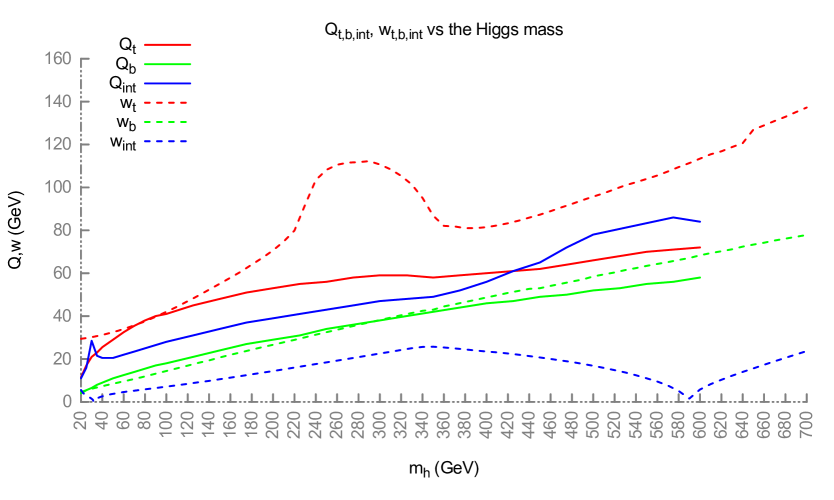
After clarifying the conceptual differences between the two approaches, we can now study the actual numerical values of the matching scales. The upper plot in Figure 3 shows the three scales for the $t$, $b$, and interference contributions for scalar Higgs production in the two approaches, with $m_{\phi}\leq 600$ GeV in the HMW case and $m_{\phi}\leq 700$ GeV in the BV case. As outlined above, while the BV scales are independent of the resummation procedure, this is not the case for HMW. The numbers shown in Figure 3 are based on AR. In principle, separate HMW matching scales should be determined for MC@NLO and POWHEG. For MC@NLO, it turns out though that the HMW scales of Figure 3 lead to numerical results close to the ones obtained in the AR approach, as the matching procedure is indeed rather similar in the two cases. On the contrary, POWHEG consistently exceeds the fixed-order $\alpha_{s}^{3}$ distribution (referred to as fNLO [Alwall:2014hca] in the following) in the high-$p_{\bot}$ tail even for very small matching scales $h$. Any HMW criterion which requires a transition to fNLO at large $p_{\bot}$ becomes questionable in this case. We therefore do not attempt to determine separate HMW scales for POWHEG, but simply use the ones of Figure 3. Let us add that the situation changes significantly when applying the so-called mPOWHEG modification, to be defined in Section 4.2.3. Similar to MC@NLO, the HMW scales of Figure 3 lead to reasonable results in this case.

Concerning the top-induced contribution, $w_{t}$ exhibits a non-trivial structure in a broad $m_{\phi}$ range around the top-quark threshold, between about $220$ and $380$ GeV. The corresponding HMW scale $Q_{t}$, on the other hand, increases quite steadily with the Higgs mass, and the top-quark threshold only has a very mild effect, if any. In addition, the overall growth of $w_{t}$ with $m_{\phi}$ is stronger than for $Q_{t}$. Nevertheless, over the whole $m_{\phi}\leq 600$ GeV region considered here, the two scales never differ by more than a factor of two. Since the resummation uncertainty in the two approaches will be estimated by varying the matching scales by a factor of two, we can expect consistent results in cases where the top contribution is dominant.

On the other hand, the BV and HMW scales for the bottom-induced contribution are in much better agreement. The BV scale $w_{b}$ exhibits a slightly steeper dependence on $m_{\phi}$ than $Q_{b}$, but the difference between the two remains quite small for all $m_{\phi}\lesssim 600$ GeV. Except for very small Higgs masses, $w_{b}$ and $Q_{b}$ are considerably larger than $m_{b}$. In the BV approach one observes that this result is driven mainly by the behavior of the partonic $gg\to\phi g$ channel [Bagnaschi:2015qta] (see also Ref. [Banfi:2013eda]), while the $qg\to\phi q$ channel would suggest a value for the bottom matching closer to $m_{b}$ [Grazzini:2013mca].

For the scales of the interference contribution, both approaches lead to a very similar slope in their respective matching scales as $m_{\phi}$ increases from about 40 to 320 GeV, even though their absolute values differ significantly. While $w_{\text{int}}$ remains below about 25 GeV, $Q_{\text{int}}$ is always larger than 20 GeV as long as $m_{\phi}\gtrsim 30$ GeV. For larger values of $m_{\phi}$, the two interference scales show a very different behavior: The BV scale $w_{\text{int}}$ slowly decreases until it reaches the value $w_{\text{int}}=0$ at about 590 GeV, which happens precisely where the interference term of the total cross section at LO vanishes. In contrast to that, the slope of the HMW scale increases beyond $m_{\phi}\approx 340$ GeV, and $Q_{\text{int}}$ assumes its maximal value of about 80 GeV at $m_{\phi}\approx 570$ GeV. A similar feature is observed around $m_{\phi}=30$ GeV. The reasons for the qualitative differences in this case have already been discussed in Section 3.3; they are the clearest manifestation of the different ideas behind the BV and the HMW method.

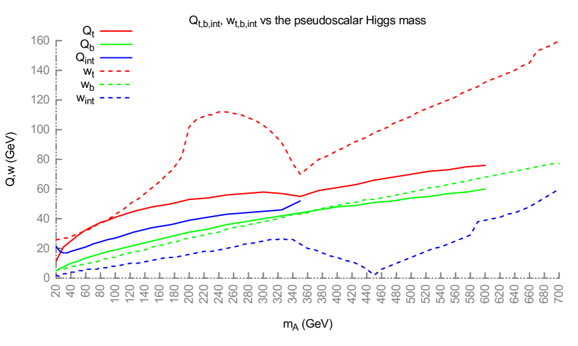
The corresponding plot for a CP-odd Higgs boson is shown in Figure 3; the general behavior for all the three contributions is quite similar to the scalar case and requires no separate discussion.

Figure 3: On the top (bottom) comparison of the matching scales in the BV and the HMW approach for the scalar (pseudo-scalar). Solid (dashed) curves correspond to the HMW (BV) scales. The scale corresponding to the top (bottom) quark squared matrix element is shown in red (green), while the values to be used for the interference term are in blue.

4 Numerical results

In this section, we present a quantitative comparison of the impact of the BV and of the HMW scale determinations, using three different codes: MoRe-SusHi, which implements the analytic resummation of the $p_{\bot}$ spectrum, gg_H_2HDM and aMCSusHi, which apply the POWHEG and the MC@NLO method, respectively. Although the theoretical basis underlying these three codes is the same, namely resummation based on soft and collinear factorization, the specific algorithms involved are quite different, see Section 2. Therefore, we will try to disentangle effects due to these different implementations from those arising from the different matching scales.

The uncertainty band due to a variation of the matching scale is obtained by the following procedure: Given a set of reference values $(\mu_{t},\mu_{b},\mu_{\text{int}})$ for the three matching scales according to Eq. (13) (adopting either the BV or the HMW approach) we consider all the possible combinations which can be generated by taking half and twice these values, or the reference values themselves; for each setting, we compute the transverse momentum distribution; collecting all these results, we take the envelope for each $p_{\bot}$ value, i.e. the minimum and the maximum values among all the simulations.

For the analytic resummation, which consistently matches the fixed-order results at large transverse momenta, we follow Ref. [1] and apply an additional factor

$$\begin{split}d(p_{\bot})=\left\{1+\exp\left[\alpha\left(p_{\bot}-m_{\phi}\right)\right]\right\}^{-1}\,,\qquad\alpha=0.1\,\mathrm{GeV}^{-1}\,,\end{split}$$ (14)

to the error band which damps it towards large values of $p_{\bot}$. This takes into account condition (a) from Section 3.1, according to which resummation should not have a big impact on the large-$p_{\bot}$ region, and thus also not on its theoretical ambiguities.

As we will see, the shape of the uncertainty band as derived from the variation of the matching scales has a feature common to all the codes. In a region just above the peak of the $p_{\bot}$ distribution, the band is relatively narrow. This is a consequence of the unitarity constraint, which establishes an anticorrelation between the low- and the high-$p_{\bot}$ tails of the distribution. The precise position of this region depends on the position of the peak of the resummed distribution, on the total variation of the cross section, as well as on the central value of the matching scale; the interplay of these factors determines the precise shape of the uncertainty band.

4.1 Setup and representative scenarios in the 2HDM

This section defines the phenomenological scenarios considered in this paper. They have been designed to highlight possible interplays between the top-quark and the bottom-quark mediated amplitudes.

We start with the SM, where the $p_{\bot}$ spectrum of the Higgs boson is known through NLO+NLL including the full dependence on the quark masses [Mantler:2012bj] and through NNLO+NNLL for the top-quark induced terms and by assuming the limit $m_{t}\to\infty$ [Bozzi:2003jy, Bozzi:2005wk, deFlorian:2011xf]. In the present study, for uniformity with the BSM codes where only NLO QCD accuracy on the total cross section and NLO+(N)LL results on the Higgs transverse momentum distribution are available, we restrict also the SM analysis to this level of accuracy.

While there is hardly any controversy that the “characteristic scale” for the top-quark induced contributions in the SM should be of the order of the Higgs boson mass ($m_{h}=125$ GeV), already in this case the BV and the HMW methods provides us with a more quantitative result for the matching scale which turns out to be close to the often adopted choice of $m_{h}/2$ in the SM, but becomes significantly smaller than $m_{\phi}$ towards larger values of $m_{\phi}$ (see Figure 3). One of the main subjects of this paper, however, is the question of how to take into account the bottom-quark induced contribution. In the SM, the effect of the bottom quark is suppressed by the Yukawa coupling, and therefore differences in this treatment have limited effect on the overall momentum distribution. In models with an extended Higgs sector, however, the bottom-quark Yukawa coupling can be significantly enhanced, at least for some of the Higgs bosons of such theories.

One of the simplest extensions of the SM in this respect is the 2HDM. Therefore, we focus on 2HDM scenarios which we devise in order to enhance specific contributions to the cross section. The conclusions of our study, however, trivially generalize to other models where the gluon-Higgs coupling is predominantly mediated by top and bottom quarks (e. g. most of the experimentally viable parameter space of the MSSM). Since the aim of this paper is a conceptual one, we disregard any phenomenological constraints on the 2HDM parameter space, in general; we do not consider the case of a light Higgs boson of mass $m_{h}=125$ GeV with enhanced bottom-quark Yukawa coupling though, due to the obvious conflict with experimental observations. We do, however, respect the theoretical constraints due to unitarity and triviality of the theory, as well as stability of the physical vacuum. We check these constraints with the help of the program 2HDMC [Eriksson:2010zzb, Eriksson:2009ws]. In all scenarios, except for the low-$m_{\scriptscriptstyle A}$ scenario to be introduced at the end of this section, we set the mass of the two CP-even Higgs bosons to $m_{h}=125$ GeV and $m_{\scriptscriptstyle H}=300$ GeV, respectively, while the mass of the CP-odd Higgs boson is set to $m_{\scriptscriptstyle A}=270$ GeV.

The first scenario we consider is “scenario B” as defined in Ref. [Harlander:2013qxa]. For consistency with the notation in the rest of this paper, however, we will refer to it as “large-$b$ scenario” in what follows. Since it induces a SM-like light Higgs boson, we only study the production of the heavy and the CP-odd Higgs boson for that scenario, both of which have strongly enhanced couplings to the bottom quark.

As a modification of this, we use the same parameters as in the large-$b$ scenario, except that we set $\tan\beta=1$. This will be referred to as “large-$t$ scenario” in what follows. It is designed to result in a top-quark dominated cross section for the heavy and pseudo-scalar Higgs boson. Again, the light Higgs is very SM-like and will not be considered in this scenario.

Finally, we devise a set of rather pathological scenarios where the LO cross section receives a large top-bottom interference contribution. The parameters of these “large-int scenarios” have to be chosen differently for each of the neutral Higgs bosons.

scenario	$\tan\beta$	$\sin(\beta-\alpha)$	$\phi$	$\sigma_{t}$/pb		$\sigma_{b}$/pb		$-\sigma_{\text{int}}$/pb
				LO	NLO	LO	NLO	LO	NLO
SM	—	—	$H$	20.027	33.400	0.220	0.268	2.410	2.433
			$A$	46.355	78.125	0.244	0.291	4.202	4.506
large-$b$	50	0.999	$H$	0.002	0.005	5.085	7.089	$0.163$	$0.199$
			$A$	0.005	0.010	9.984	13.408	0.334	0.412
large-$t$	1.0	0.999	$H$	3.715	6.788	0.002	0.003	$-0.132$	$-0.168$
			$A$	12.844	23.832	0.004	0.005	0.334	0.428
large-int	3.2	$-0.6$	$h$	2.453	4.091	2.192	2.674	$2.665$	$2.677$
	7.1	$-0.26$	$A$	0.255	0.473	0.201	0.270	$0.334$	$0.430$
low-$m_{\scriptscriptstyle A}$	36.9	$0.998$	$A$	0.399	0.552	$2.480\cdot 10^{5}$	$2.292\cdot 10^{5}$	89.70	$-693.6$

Table 1: Cross sections for the three 2HDM scenarios considered in our study, obtained with SusHi (the integration error at NLO is of the order of 0.1%, and negligible at LO). See the text for a description of their characteristics.

The precise definition of all scenarios, together with the top-, bottom- and interference component of the total inclusive cross sections at LO and NLO, is given in Table 1. Note that, while for the light and the pseudo-scalar Higgs the absolute value of the interference term in the large-int scenarios amounts to more than 100% of the total cross section, we did not manage to find a parameter point for the heavy Higgs which has a similarly large interference term while still respecting the theoretical constraints of unitarity, stability, and perturbativity.

Let us emphasize again that most of these scenarios are in vast conflict with experimental observations; they only serve as theoretical benchmarks for the study of resummation ambiguities in the Higgs $p_{\bot}$ distribution. For phenomenologically viable 2HDM benchmark points we refer the reader to Ref. [Haber:2015pua].

We further investigate one phenomenologically interesting scenario with a very low pseudo-scalar Higgs boson mass. In this case we chose a scenario of Ref. [Bernon:2014nxa] that meets all theoretical as well as experimental constraints. This scenario is referred to as low-$m_{\scriptscriptstyle A}$ in Table 1. The masses of the three Higgs bosons are $m_{h}=125.5$ GeV, $m_{\scriptscriptstyle H}=507$ GeV and $m_{\scriptscriptstyle A}=29.9$ GeV. For such a low Higgs-boson mass, the gluon-fusion process is particularly important, since its cross section is highly enhanced with respect to Higgs production in association with bottom quarks and dominant even at large $\tan\beta$ [Bernon:2014nxa].

All the numerical results are computed for the LHC, with a center-of-mass energy of $\sqrt{S}=13$ TeV. We use the MSTW2008nlo68cl PDF set [Martin:2009iq] through the LHAPDF6 library [Buckley:2014ana] and the corresponding value of $\alpha_{s}(M_{Z})=0.120179$. The renormalization and factorization scales are both identified with $m_{\phi}$. The pole masses of the top and the bottom quark are fixed at $m_{t}=172.5$ GeV and $m_{b}=4.75$ GeV, respectively. We used the on-shell renormalization scheme for the Yukawa couplings. For simulations involving a parton shower, we apply Pythia8 [Sjostrand:2007gs].

4.2 Numerical results in the different scenarios

This section contains the results obtained with the three codes under study, in the various scenarios defined in Section 4.1. Since our focus is on the uncertainties inherent to the matching procedure, we compute the uncertainty band by varying only the matching scales, as described in Section 4.

For each scenario we performed two different studies:

1. The predictions for AR, MC@NLO and POWHEG are compared by using the same numerical values for the respective matching scales; in this way we can assess the impact of the higher-order QCD terms which are included in different ways in the three codes, due to the different matching procedures.

2. For each code, the predictions obtained by setting the matching scale to the BV and to the HMW values are compared; this allows us to assess the sensitivity of each code to a matching scale variation, the impact of the BV vs. the HMW prescription, and the overlap of the respective uncertainty bands.

4.2.1 Results in the Standard Model

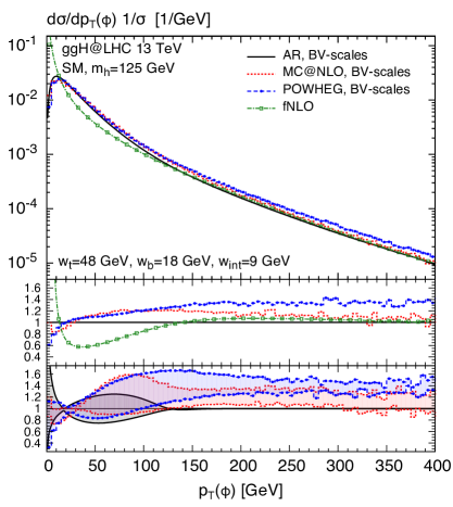
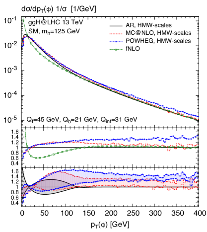
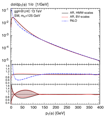
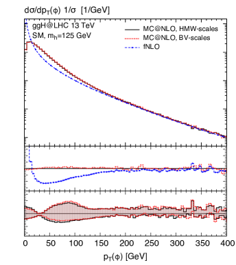
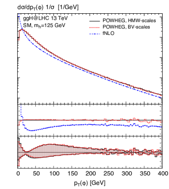
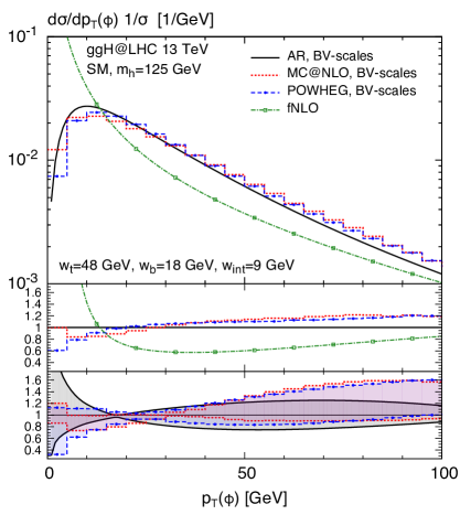
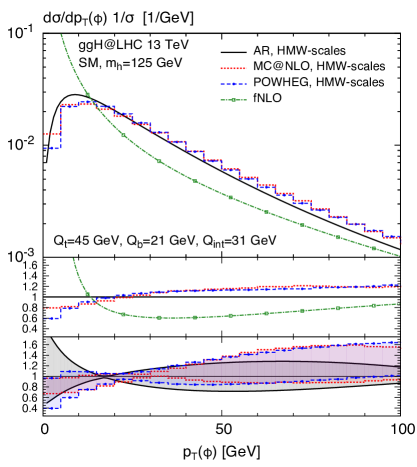
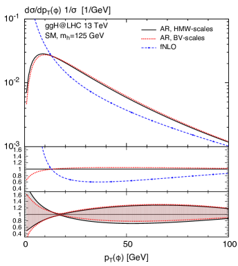
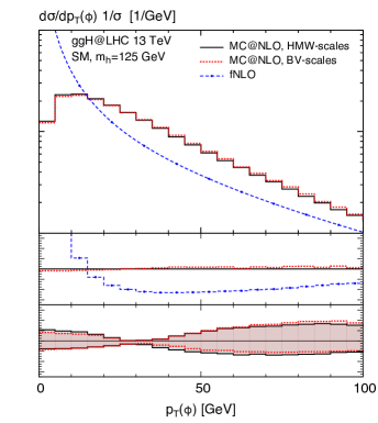
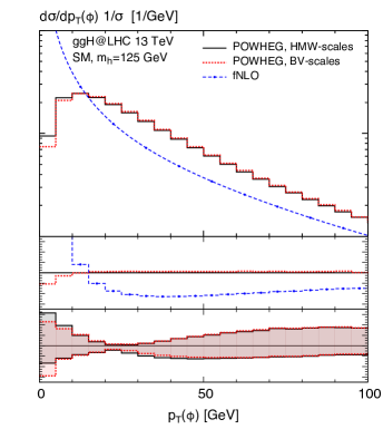
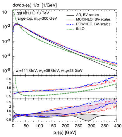
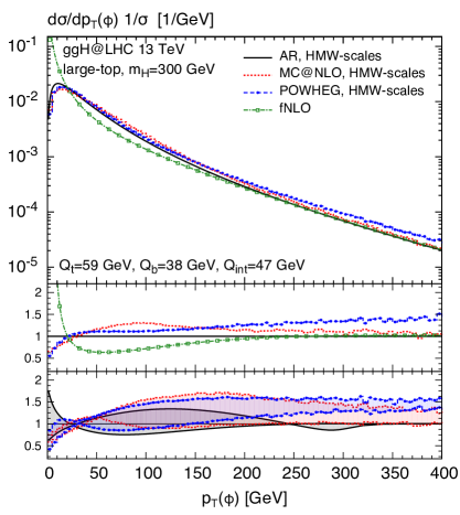
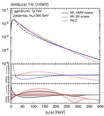
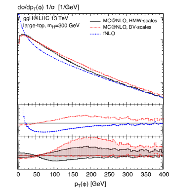
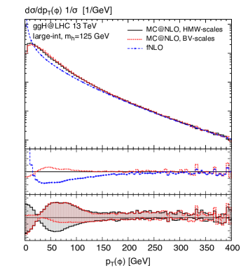
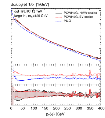
Even though for the SM one may expect consistency among the three codes, it will be instructive to start our discussion with this case, because it highlights certain generic features of the individual approaches which will be carried forward also to some of the other scenarios considered in this paper. Figure 4 shows the shape of the transverse-momentum distribution (i.e., the integral of each curve is normalized to one) for a SM Higgs of $m_{h}=125$ GeV in the range $0\leq p_{\bot}/{\rm GeV}\leq 400$. In the two upper plots, we compare the results of the three codes, setting the matching scales to the same numerical values: BV scales in the left and HMW scales in the right panel (cf. item i) above). Each of the lower plots, on the other hand, was obtained with one particular code (left: AR; center: MC@NLO; right: POWHEG); the different lines correspond to different values of the matching scales, BV and HMW (cf. item ii) above). All plots contain the fNLO result as a reference. In order to facilitate the discussion, we show the same plots in Figure 5, but with enlarged low-$p_{\bot}$ region ($0\leq p_{\bot}/{\rm GeV}\leq 100$).

Apart from the fact that, as expected, the three codes yield compatible results within uncertainties (at least for $p_{\bot}\leq m_{h}$), it is worth noting the following characteristics:

• The central POWHEG and the MC@NLO spectra are in excellent agreement (at the few-percent level) between about $10<p_{\bot}/\text{GeV}<130$, while they differ by about 20% from the central AR prediction in most of this region.

• The peak position for both POWHEG and MC@NLO is at around $p_{\bot}=12$ GeV, while the peak for AR is about 2 GeV below that.

• The central value of AR approaches fNLO at the level of $\lesssim$ 5% above $p_{\bot}\approx 130$ GeV; for MC@NLO, such a transition to the fixed-order curve occurs at about $p_{\bot}\approx 180$ GeV, while POWHEG always remains about 20% above fNLO in the tail of the distribution. The latter characteristic is a general feature of the default POWHEG matching, as described in Section 2.2.2, and will be analyzed in detail in Section 4.2.3.

• Above $p_{\bot}\approx 130$ GeV, the uncertainty band for AR is suppressed due to the damping factor introduced in Eq. (14). Concerning the two MCs, in MC@NLO the uncertainty, expressed in unit of the AR central value, is of the order of $\pm 10\%$ from $p_{\bot}=130$ GeV all the way up to $p_{\bot}=400$ GeV, while for POWHEG it decreases uniformly from $\pm 20$% to $\pm 10$%.

• The MC@NLO and POWHEG bands nicely overlap for $p_{\bot}\leq 100$ GeV; above this value the overlap is only partial, because of the different central predictions.

• Towards smaller values of $p_{\bot}$, the uncertainty bands for all three codes develop a bulgy structure with a maximum of about $\pm 20\%$ $(\pm 35\%)$ for AR (the Monte Carlos) and a minimum of a few percent slightly above the peak position.

• Towards even smaller values of $p_{\bot}$, the AR uncertainty band quickly grows to the 100% level, and the POWHEG band to about $\pm 40\%$. Only the MC@NLO band increases to a moderate $\pm 15\%$.

Since, for a SM Higgs of $m_{h}=125$ GeV, the BV and HMW scales are quite close to each other (see Figure 3), the two upper plots in Figure 4 are very similar. In order to see this more explicitly, we study the impact of the different scale choices (BV or HMW) within one particular code (left: AR; right: MC@NLO) in the lower three plots of Figure 4. From the latter we can indeed see that the results obtained in the two cases are in very good agreement with each other, both with respect to the central value and the uncertainty band; the only difference being at very low transverse momenta ($p_{\bot}{}<10$ GeV) in the central predictions of AR and POWHEG. This can be traced back to the different matching scales for the interference term, which constitutes the largest contribution induced by the bottom-quark loop in the SM.

Figure 4: Shapes of the transverse-momentum distributions (i.e., normalized such that the integral yields one) for a SM Higgs boson with $m_{h}=125$ GeV. In the upper plots we show the distributions computed with AR (black, solid), MC@NLO (red, dotted) and POWHEG (blue, dashed overlaid by points), setting the matching scales to the BV values (left) or the HMW values (right). For reference, we also show the fixed-NLO (fNLO) prediction (green, dash-dotted with open boxes). The main frame shows the absolute distributions, the first inset the shape-ratio of the central values to the AR distribution, and the second inset the uncertainty bands, normalized again to the central AR value. In the lower three plots we compare the results within each code, using for the matching scales the BV values (red, dotted) and the HMW values (black, solid), taking the HMW results as reference for the ratios of the insets.

Figure 5: Same as Figure 4, but with enlarged low-$p_{\bot}$ region.

4.2.2 Results in the large-$t$ scenario

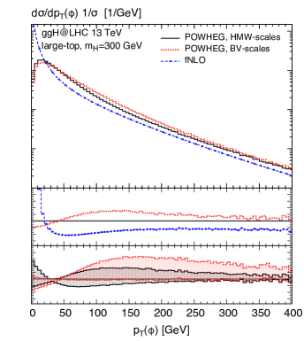
Let us now consider the production of a heavy Higgs with $m_{\scriptscriptstyle H}=300$ GeV in the large-$t$ scenario, where, similar to the SM, the bottom-loop and the interference contribution play only a minor role. In contrast to the SM, however, the matching scales for the top-loop contribution derived using BV and HMW differ by almost a factor of two. The results for the $p_{\bot}$ distribution are shown in Figure 6.

Using BV scales, one notices that AR deviates quite significantly ($\sim 50$%) already at $p_{\bot}{}=400$ GeV from the fNLO result; this deviation tends to further increase towards larger $p_{\bot}$ values. This is not unexpected since the HMW scales are designed to guarantee similarity between the resummed and the fNLO curve at large $p_{\bot}$. Scale choices larger than the values determined by HMW will therefore necessarily lead to a deviation from the fNLO in that region. In the case of POWHEG and MC@NLO, their canonical high-$p_{\bot}$ behavior starts to appear only for relatively large values of $p_{\bot}$, the reason for this being again the relatively high value of the scale for the top contribution ($w_{t}=111$ GeV). Indeed, the agreement between the two Monte Carlos turns out to be excellent, at least up to $p_{\bot}$ values as large as the Higgs mass. Despite the large deviations of AR in the tail and the much softer AR spectrum, all approaches are compatible within uncertainties at small to intermediate transverse momenta ($p_{\bot}{}\lesssim 200$ GeV). It should be noted that this is partly due to the fact that the uncertainty bands are significantly larger (almost by a factor of two) than in the SM.

Using HMW scales, the transition to the high-$p_{\bot}$ region is more similar to the SM case (including the consistent overshooting of the POWHEG spectrum) because of the relatively flat dependence on the Higgs mass of the HMW scales, implying $Q_{t}^{\text{large-t}}/Q_{t}^{\text{{SM}}}\simeq 1.3$. The results from the three codes appear to be more compatible, in particular in the tail of the distributions, mainly due to the different AR behavior. The bulges of the uncertainty bands above the peak position extend to considerably larger values of $p_{\bot}$, and their width is similar to what we observed for the SM.

Despite the apparent differences between the left and the right upper plots, the dedicated analysis of the impact of the scales choice in the lower plots reveals that the results are nicely compatible within the respective uncertainty bands. The only exception from this occurs for AR at large $p_{\bot}$. But one should bear in mind that the uncertainty band for AR is manually suppressed at large $p_{\bot}$, a procedure that should strictly be applied only when HMW scales are used. The observation that the width of the BV-bands is larger than for HMW is due to the fact that $w_{t}$ is more than twice as large than $Q_{t}$, and thus the variation by a factor of two has a bigger impact on the final result.

The results for the CP-odd Higgs boson in the large-$t$ scenario are very similar to the ones of the heavy CP-even Higgs shown here. We therefore refrain from showing them here.

Figure 6: Same as Figure 4, but for a 2HDM  heavy scalar Higgs boson with $m_{\scriptscriptstyle H}=300$ GeV in the top dominated scenario.

4.2.3 Results in the large-$b$ scenario

The large-$b$ scenario produces large bottom-Yukawa couplings for the heavy and the pseudo-scalar Higgs boson which renders the bottom-loop induced contribution by far dominant. Since the associated matching scales $w_{b}$ and $Q_{b}$ are very close to each other, any difference in the $p_{\bot}$ distributions are due to the conceptional variants of the matching in the three codes under consideration. Figure 7 shows the results for a heavy Higgs boson using HMW scales (the corresponding plots for BV scales are identical for all practical purposes).

Figure 7: The first plot is the same as the upper right plot of Figure 4, but for a 2HDM  heavy scalar Higgs boson with $m_{\scriptscriptstyle H}=300$ GeV in the bottom dominated scenario. The other plots show two additional curves: MC@NLO applying a fixed value ($\delta$-distribution) to the shower scale of each contribution using the HMW values (orange, solid with full boxes); a modified-POWHEG (mPOWHEG) approach requiring emissions in all remnant events to be bounded by the matching scales (HMW in this case) from above (magenta, solid with stars).

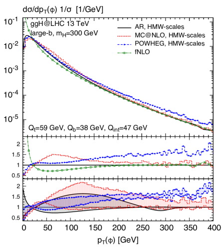
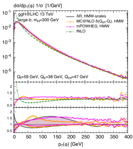
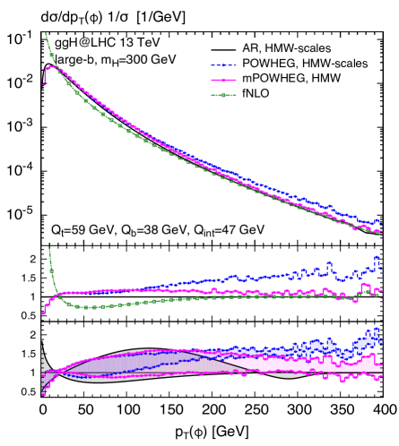
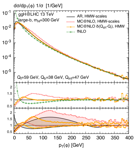
Let us first discuss the upper left plot of Figure 7, where the curves are displayed in the same way as in the corresponding plots of Figure 4 and Figure 6 for the SM and the large-$t$ scenario, respectively. While the large-$p_{\bot}$ behavior for AR and MC@NLO is similar to the large-$t$ scenario, POWHEG produces a spectrum that is significantly harder, exceeding the fNLO result by about 50% for $p_{\bot}\gtrsim 200$ GeV. Apparently, the specific matching procedure of POWHEG has a significant impact on the large $p_{\bot}$ region, where the parton shower, based on the soft/collinear approximation, is outside its region of validity. Between $10\lesssim p_{\bot}/\text{GeV}\lesssim 130$, on the other hand, POWHEG and AR agree within 10%, while MC@NLO is significantly higher in that region. The central predictions of the two Monte Carlo results are in reasonable agreement only at small transverse momenta ($p_{\bot}\lesssim 30$ GeV). Moreover, the size of the error bands is very different in the two Monte Carlo approaches: the MC@NLO band blows up to ${\cal O}(100\%)$ around $p_{\bot}{}\sim 125$ GeV; the POWHEG band remains very narrow over the whole range, indicating an uncertainty even smaller than in the SM. The fact that all approaches lead to compatible predictions below $p_{\bot}\approx 200$ GeV is mainly due to the large MC@NLO band.

Since the large-$b$ scenario reveals the differences between the three codes under study in the most striking way, it will be instructive to investigate them in more detail within this scenario. Consider first the POWHEG approach. As it turns out, both observed features—enhanced high-$p_{\bot}$ tail and small uncertainty band—can be tackled by the same modification of the matching procedure: In the original POWHEG approach, the scale $t_{1}$ (see Section 2.2) for each event is identified with the transverse momentum of the first emission. If the latter is very large, the shower will act up to scales which are way beyond the validity range of the underlying approximations. If instead we restrict $t_{1}$ for all remnant events (the $R^{f}$-term in Eq. (6)) to remain below the matching scale (e.g. BV or HMW), one obtains the result shown in the lower left plot of Figure 7 (magenta, solid curve with stars). Since the high-$p_{\bot}$ tail of the distribution is driven by the remnant events, the above restriction of $t_{1}$ ensures a transition to the fNLO curve. We will refer to this modified approach as “mPOWHEG” in what follows. It happens that also the uncertainty band is more similar to the other approaches for the mPOWHEG result (see again the lower left plot of Figure 7).

The fact that the mPOWHEG modification applies only to the remnant events ensures that the formal accuracy of the original POWHEG approach remains unaffected. In this respect, it is reassuring that at low transverse momenta ($p_{\bot}\lesssim 100$ GeV), the modifications have practically no effect (compare the POWHEG with the mPOWHEG curve in Figure 7), as this region is controlled by the soft events (the first term in Eq. (6)), which remain unchanged. We checked that the fNLO-like high-$p_{\bot}$ behavior of mPOWHEG is a generic feature and not specific to the underlying phenomenological scenario or the details of the parton shower. A more quantitative study of its numerical impact has to be deferred to a future study though. Stressing again that, to our understanding, mPOWHEG is only a logarithmically subleading modification of POWHEG (or rather its interface with the parton shower), one may consider it as a viable alternative whenever an fNLO-like high-$p_{\bot}$ behavior is required.

Let us now discuss the MC@NLO approach in this scenario, featuring a peculiarly large uncertainty regarding shower scale variations, which in turn leads to very different shapes of both the central predictions and the error band with respect to the other two approaches. Recall that in the MC@NLO implementation of MadGraph5_aMC@NLO, the values for the shower scale of the soft events follow a specific distribution with a peak at the matching scale $\mu_{i}$ ($i=t,b,\text{int}$; e.g. BV or HMW), see Section 2.2.1. We find that, in the large-$b$ scenario, a restriction of the range of that distribution has a significant effect on the central MC@NLO prediction, which is not surprising given the large associated uncertainty. In the limit where this distribution turns into a $\delta$-function $\delta(Q_{\text{sh}}{}-\mu_{i})$, also the size of the uncertainty band is strongly reduced, as can be seen in the lower right plot of Figure 7 (orange, solid curve with full boxes). We checked that, besides a slightly earlier matching to the fNLO prediction controlled by the remnant events, the observed features are due to the restricted shower scale range accessible to the soft events. This study simply shows that the predictions in bottom-quark dominated scenarios depend strongly on details of the matching procedure and thus should be attributed with large uncertainties.

Finally, the upper right plot of Figure 7 shows the comparison of the results obtained with the modifications done for MC@NLO and POWHEG. Indeed, the modified predictions turn out to be in much better agreement, in terms of both the central curves and the uncertainty bands.

Similar to the large-$t$ scenario, the distributions for the pseudo-scalar Higgs in the large-$b$ scenario largely resemble the ones of the heavy Higgs shown in Figure 7, and we do not need to discuss them separately at this point.

4.2.4 Results in the large-int scenario

The matching scales of the interference term in the BV and the HMW approach exhibit quite a different behavior, as shown in Figure 3. It will thus be interesting to see the distributions in the various approaches in a scenario with a particularly large interference term. Note, however, that the interference term in the large-int scenarios defined in Table 1 is always negative and competes with a similarly large top and/or bottom contribution. Our 2HDM parameter scan did not reveal a truly interference-dominated scenario, where both the top and the bottom contribution are small compared to the interference term, and which passes the unitarity, stability, and perturbativity checks.

Figure 8 shows the results for the light Higgs boson, where the modulus of the top, the bottom, the interference term, and the total cross section each are roughly of the same size ($\sim 2$ pb, see Table 1). Note that the top and the bottom matching scales agree well in the BV and the HMW approach for the light Higgs, while the interference matching scale is about a factor of three larger in the HMW approach.

Using HMW scales, the comparison of the distributions in the various approaches leads to a picture that is quite similar to the one that we found in the SM: good agreement among the Monte Carlos, softer spectrum of AR, compatible results within uncertainties of all approaches (at least for $p_{\bot}\leq m_{h}$). The error bands, on the other hand, are significantly larger than in the SM. They amount up to about $\pm 60\%$ for AR and MC@NLO, and about $\pm 40\%$ for POWHEG.

Figure 8: Same as Figure 4, but for a 2HDM  light scalar Higgs boson with $m_{\scriptscriptstyle H}=125$ GeV in the large interference scenario.

Figure 9: Left: same as upper left plot of Figure 8, but with enlarged low-$p_{\bot}$ region. Right: Same scenario and notation, but for a pseudo-scalar Higgs boson with $m_{\scriptscriptstyle A}=270$ GeV.

Figure 10: Same as Figure 4, but for a 2HDM  pseudo-scalar Higgs boson with $m_{\scriptscriptstyle A}=270$ GeV in the large interference scenario.

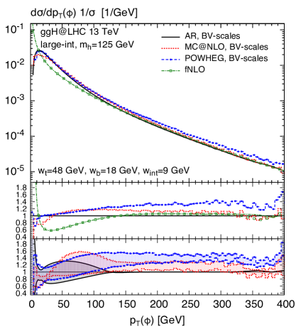
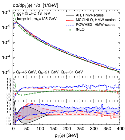
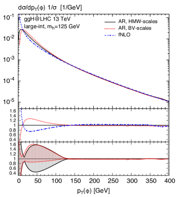
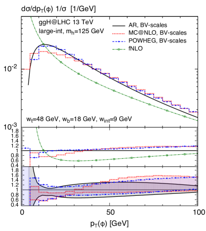
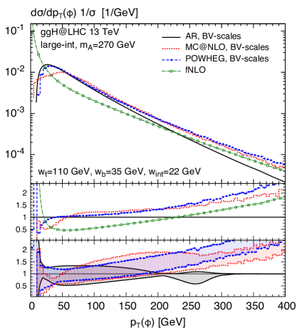
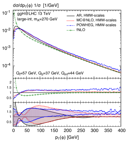
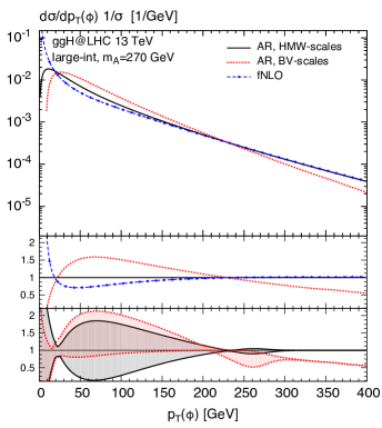
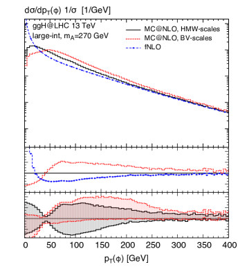
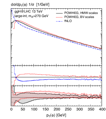
Using BV scales, on the other hand, the width of all uncertainty bands is strongly reduced (up to about $\pm 20\%$ and $\pm 30\%$ for AR and the Monte Carlos, respectively), the reason being again the fact that a large $Q_{\text{int}}$ (as in HMW) also induces a large interval $[Q_{\text{int}}/2,2Q_{\text{int}}]$. While also for BV the results at small $p_{\bot}$ are compatible within uncertainties and the high-$p_{\bot}$ behavior is very reminiscent of the one observed in the SM, there are some substantial differences at very small transverse momenta ($p_{\bot}{}<40$ GeV) between the shapes predicted by the two Monte Carlos. For better visibility, Figure 9 shows in the left panel the BV plot with an enlarged low-$p_{\bot}$ region. Clearly, the MC@NLO spectrum is harder, while the POWHEG one actually gets negative in the first bin. Since the interference term is not positive definite, due to its definition by subtraction, the distribution may turn negative in scenarios where its contribution is large. Clearly, this behavior appears to be amplified at small $p_{\bot}$ if the matching scale is particularly small. At least this specific case, therefore, leads to a similar conclusion as pointed out in Ref. [Mantler:2015vba], that very low scales are not well suited for NLO matched parton shower predictions.

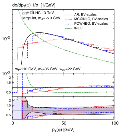
Indeed, the behavior just observed is even enhanced in the large-int scenario of the pseudo-scalar Higgs with $m_{\scriptscriptstyle A}=270$ GeV, see Figure 9 (right panel). The MC@NLO distribution displays some odd behavior between about $10<p_{\bot}{}/{\rm GeV}<60$, developing an almost linear behavior rather than the ordinary Sudakov shoulder. The POWHEG prediction, on the other hand, becomes negative in the first and the second bin of the distribution (i.e., below $p_{\bot}=10$ GeV). There are mainly two reasons for these features being intensified in the large-int scenario of the pseudo-scalar Higgs: First, the ratio of the interference matching scale to the Higgs mass is even smaller than for the light Higgs; second, the relative contribution of the interference term is larger than in the light Higgs case. The latter can be inferred from Table 1: For the pseudo-scalar Higgs, the large-int scenario corresponds to an interference term whose modulus is about 30% larger than the top, 50% larger than the bottom contribution, and 270% larger than the total cross section.

The other results in the large-int scenario of the pseudo-scalar Higgs are shown in Figure 10. The conclusions are essentially the same as the ones for the light Higgs, which will thus not be repeated here. It is worth mentioning though that the relative size of the uncertainty bands for both BV and HMW scales are increased with respect to the light Higgs case, the reason being again the larger value of the matching scale and the thereby enlarged variation range.

4.2.5 Results in the low-$m_{\scriptscriptstyle A}$ scenario

Also the low-$m_{\scriptscriptstyle A}$ scenario produces large bottom-Yukawa couplings, but in this case the Higgs and the bottom mass are significantly closer than in the large-$b$ scenario. Thus, all contributions besides the bottom-loop induced one are negligible and $Q_{b}$ is quite close to $w_{b}$. Figure 11 shows, therefore, only the comparison among the three codes for the BV scales, while the corresponding HMW results are identical for all practical purposes.

Figure 11: Same as Figure 7, but for BV scales and a 2HDM  pseudo-scalar Higgs boson with $m_{\scriptscriptstyle A}=30$ GeV in the low-$m_{\scriptscriptstyle A}$ scenario.

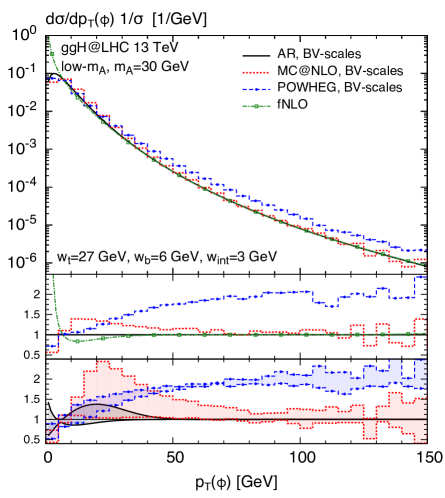
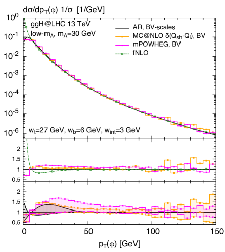
Looking first at the left plot in Figure 11, we notice that the characteristic features observed in the large-$b$ scenario appear to be amplified in this case: the MC@NLO uncertainty band blows up to ${\cal O}(150\%)$ around $p_{\bot}{}\sim 25$ GeV; the POWHEG curve exceeds the fNLO result by about 100% for $p_{\bot}\gtrsim 50$ GeV with a very small uncertainty band. The central curves are vastly different between the two Monte Carlo approaches except for the first two bins.

In the right plot of Figure 11 we show the corresponding curves for the modified approaches (MC@NLO with fixed shower scale, mPOWHEG). Evidently, the agreement among the results is significantly improved. Also in this case, a restriction of the shower scale in POWHEG closes the large gap to fNLO in the tail of the distribution, such that the mPOWHEG curve nicely approaches fNLO at large $p_{\bot}$. The MC@NLO uncertainty band is very similar to the one of AR and the central predictions of the Monte Carlos are almost on top of each other. Note that for such small Higgs boson masses, the shower scale distribution as defined in Section 2.2.1 ranges down to very low values ($Q_{\text{sh}}{}\sim 1$ GeV) which are not well suited for a Monte Carlo approach, both from a physical and a technical point of view. This can be avoided by using narrower distributions—a $\delta$-function in our case—for $Q_{\text{sh}}{}$, thus leading to a better agreement with the other codes and a more reasonable size of the uncertainty band.

5 Conclusions

A reliable theoretical prediction of the Higgs transverse-momentum distribution must include an estimate of the uncertainties associated with the matching of fixed- and all-order results. The latter are relevant to describe the large- and the low-$p_{\bot}$ parts of the spectrum, respectively. The matching procedure is not unique; in this paper, we studied three different methodological approaches and their dependence on the respective matching scale.

In general, the gluon-fusion process is characterized by two external, physical scales: the mass of the Higgs boson and the mass of the quark running in the loop of the gluon-gluon-Higgs vertex. Since in the SM, where the top quark is dominant, these two scales are quite close to each other, the issue of setting the matching scale is less problematic. In BSM scenarios with enhanced bottom Yukawa coupling, however, the proper choice of the matching scale has become a matter of debate.

In this paper we presented two distinct comparisons:

1. The determination of a suitable central value for the matching scales associated to the top, bottom, and interference terms, as proposed in the HMW [1] and BV [Bagnaschi:2015qta] approaches, is compared qualitatively and quantitatively. Figure 3 summarizes the main outcome as a function of the Higgs mass, both for a CP-even and a CP-odd Higgs boson.

2. The predictions of three resummation codes to the problem of the matching (AR, MC@NLO and POWHEG), all at NLO QCD accuracy concerning their normalization, but different in their logarithmic accuracy, are compared at the level of their central values and of the respective uncertainty bands, obtained through variation of the matching parameter by a factor of two around a central value. The latter has been fixed following the prescriptions of point $i)$. In this comparison we considered the production of a Higgs boson in the framework of the SM and a number of 2HDM scenarios which are representative of the different possible interplays between top- and bottom-quark effects in the gluon-fusion scattering amplitude.

In these comparisons, it is important to keep in mind that resummation considerably improves the theoretical prediction in the low-$p_{\bot}$ region, while one cannot expect the resummed (and matched) result to be in any way superior to the fixed-order prediction at intermediate and high-$p_{\bot}$. We showed that the discrepancies among the codes outside the low-$p_{\bot}$ region can be greatly reduced by a modification of the treatment of formally subleading logarithmic terms.

In the low-$p_{\bot}$ region, we find very compatible results among the three codes in all scenarios, independent of whether one uses BV or HMW scales. Even in cases where the central scales suggested by the two methods differ relatively strongly, the respective $p_{\bot}$ distributions are consistent with each other once their error band is taken into account. For the interference term, this reflects the complementary reasoning behind the BV and HMW methods which allows them to diverge as long as the sensitivity of the $p_{\bot}$ distribution on the matching scale is small.

Let us summarize the outcome of our study as follows:

• The matching uncertainty on the prediction of the Higgs transverse momentum distribution amounts to one up to several tens of percent, depending on the specific value of $p_{\bot}$ and on the model under study. This uncertainty should be combined with the usual perturbative uncertainty estimated via renormalization and factorization scale variations.

• As far as small transverse momenta are concerned, we find reasonable agreement among the codes irrespective of the specific matching scale choice (BV or HMW), although the central AR result shows a generally much softer spectrum as compared to the central prediction of the Monte Carlo codes. The agreement among the three codes is in part caused by an increase of their error band towards very low $p_{\bot}$ (essentially in the first 5 GeV bin of the distribution), which is most apparent though for the AR result. Note, however, that the cross section is typically very small in this region. Let us recall that these results have been obtained with the Pythia8 parton shower; variations with the parton shower are left for future studies.

• In the intermediate $p_{\bot}$ range, the estimate of the width of the matching uncertainty bands shows differences in the three approaches under study, which are more pronounced in the bottom dominated scenarios. In this last case the size and shape of the uncertainty bands strongly depends on the matching formulation, as it has been explicitly shown in the MC@NLO case with the use of different probability functions to extract the value of the shower scale.

• In the large $p_{\bot}$ range, where all the codes have only LO accuracy, sizable differences appear in their predictions, where the POWHEG result is systematically larger than the MC@NLO and AR curves, which in turn are compatible with the fNLO one. One source of this discrepancy has been identified in the different treatment of high-$p_{\bot}$ multiple parton emissions beyond the first one, still allowed in POWHEG and suppressed in the other two cases. We expect the precise size of the discrepancy to depend on the details of the parton shower; quantitative studies will be deferred to a future publication. The codes compared in this note provide either a transition to the LO prediction at large $p_{\bot}$ (AR and MC@NLO), which has a well defined perturbative accuracy, but misses the effects of additional radiation, or a prediction that includes multiple parton emissions at all transverse momenta, but describes them by means of a PS (POWHEG), which is not adequate at large $p_{\bot}$ because it is based on the soft/collinear approximation. It was shown that a simple modification of the interface between POWHEG and the PS (referred to as mPOWHEG in the text), which restricts the shower scale of the remnant events, can be applied to ensure a consistent matching to the fNLO prediction in the tail of the distribution, similar to the other two approaches.

The approaches studied here do not lead to identical results; not only their central values, but also their matching-induced uncertainty bands show characteristic differences. Nevertheless, it is fair to say that, in the low-$p_{\bot}$ region and including these error estimates, the results obtained by following either the BV or the HMW approach, and by employing either of the three codes are consistent with each other. This allows the conclusion that any of these approaches leads to a valid prediction for the low-$p_{\bot}$ distribution once the matching as well as the perturbative uncertainties are taken into account. The former should be estimated by a variation of the respective matching scale around its central value, as given by BV or HMW, the latter by a variation of the renormalization and factorization scales. In the intermediate- and high-$p_{\bot}$ region, where large PS effects become quite doubtful, all approaches can be made compatible with the fNLO result by suitable minor modifications.

Let us point out that the new generation of Monte Carlo event generators, merged at NLO+PS [Frederix:2012ps, Hoeche:2014lxa, Buschmann:2014sia] or NNLO QCD accurate for quantities inclusive over the radiation [Hamilton:2013fea, Hoche:2014dla, Hamilton:2015nsa, Alioli:2013hqa, Alioli:2015toa], with NLO QCD accuracy in the description of the Higgs transverse momentum spectrum, offers a more accurate description of the $p_{\bot}$ spectrum, however only in the SM-like scenario. The evaluation of the associated matching uncertainties is left to a future study.

Appendix A Numerical values of the matching scales

In the appendix we include two tables with the values of the matching scales as computed in the HMW and BV approaches, for both a scalar and a pseudo-scalar Higgs boson. The top-quark pole mass has been set to $172.5$ GeV, while the bottom-quark pole mass is assumed to be equal to $4.75$ GeV. Both sets of scales are dependent on inputs at the hadron level. For HMW this is due to the fact that the scales are determined using resummed hadronic cross sections, while in the BV procedure, hadronic physics enters in the merging of the two sets of scales obtained separately for the $gg$ and $qg$ channels. This implies the existence of a (minimal) dependence on the center-of-mass energy and on the PDF set used in the determination. For our study we have chosen $\sqrt{S}=13$ TeV and we have used the MSTW2008nlo68cl PDF set.

$m_{h/H}$ [GeV]	HMW [GeV]			BV [GeV]
	$Q_{t}$	$Q_{b}$	$Q_{int}$	$w_{t}$	$w_{b}$	$w_{int}$
20	11.5	4	11	29	5	6
25	17	5.5	16	30	5	3
30	21	6.5	28.5	30	6	1
35	23	8	21.5	31	7	2
40	25.5	9	20.5	31	7	3
50	29	11	20.5	33	8	4
60	32.5	12.5	22	34	10	5
70	35.5	14	23.5	36	11	5
80	38	15.5	25	38	12	6
90	40	17	26.5	40	13	6
100	41	18	28	42	14	7
125	45	21	31	48	18	9
150	48	24	34	55	21	11
175	51	27	37	62	24	12
200	53	29	39	71	27	14
225	55	31	41	85	29	16
250	56	34	43	108	32	18
275	58	36	45	112	35	20
300	59	38	47	111	38	23
325	59	40	48	103	41	25
350	58	42	49	87	43	26
375	59	44	52	81	46	25
400	60	46	56	81	49	23
425	61	47	61	84	51	22
450	62	49	65	87	53	21
475	64	50	72	91	56	19
500	66	52	78	96	58	17
525	68	53	–	100	61	14
550	70	55	–	104	63	11
575	71	56	86	108	66	6
600	72	58	84	113	68	6

Table 2: Table of the matching scales (in GeV) in the HMW and BV approach for a CP-even Higgs boson. A dash is used to indicate the case where the determination procedure of a scale has not been successful.

$m_{A}$ [GeV]	HMW [GeV]			BV [GeV]
	$Q_{t}$	$Q_{b}$	$Q_{int}$	$w_{t}$	$w_{b}$	$w_{int}$
20	11.5	5	21.5	26	5	2
25	16.5	6.5	18	26	6	1
30	21	7.5	17	27	6	3
35	23	9	17	27	7	3
40	25	10	18	28	8	4
50	29	11.5	19.5	30	9	5
60	32.5	13.5	21	32	10	6
70	35	15	23	34	11	6
80	37.5	16.5	24.5	37	12	7
90	39	18	26	40	13	7
100	41	19	27	43	14	8
125	45	22	31	52	18	10
150	48	25	34	61	21	12
175	50	28	36	72	24	14
200	53	31	39	102	27	16
225	54	33	41	110	30	18
250	56	36	43	112	33	20
275	57	38	44	109	35	23
300	58	40	45	103	38	25
325	57	42	46	91	41	27
350	55	44	52	70	43	23
375	59	46	–	80	46	18
400	61	48	–	86	49	14
425	63	49	–	92	51	10
450	66	51	–	98	53	2
475	68	52	–	104	55	9
500	70	54	–	109	58	14
525	72	55	–	115	61	19
550	73	57	–	120	63	23
575	75	58	–	126	65	28
600	76	60	–	132	68	39

Table 3: Table of the matching scales (in GeV) in the HMW and BV approach for a CP-odd Higgs boson. A dash is used to indicate the case where the determination procedure of a scale has not been successful.

References

- [1] R.V. Harlander, H. Mantler, and M. Wiesemann, Transverse momentum resummation for Higgs production via gluon fusion in the MSSM, JHEP 1411, 116 (2014)