CMB all-scale blackbody distortions induced by linearizing temperature
Abstract
Cosmic Microwave Background (CMB) experiments, such as WMAP and Planck, measure intensity anisotropies and build maps using a linearized formula for relating them to the temperature blackbody fluctuations. However, this procedure also generates a signal in the maps in the form of y-type distortions which is degenerate with the thermal Sunyaev Zel’dovich (tSZ) effect. These are small effects that arise at second-order in the temperature fluctuations not from primordial physics but from such a limitation of the map-making procedure. They constitute a contaminant for measurements of: our peculiar velocity, the tSZ and primordial -distortions. They can nevertheless be well-modeled and accounted for. We show that the distortions arise from a leakage of the CMB dipole into the -channel which couples to all multipoles, mostly affecting the range . This should be visible in Planck’s -maps with an estimated signal-to-noise ratio of about 12. We note however that such frequency-dependent terms carry no new information on the nature of the CMB dipole. This implies that the real significance of Planck’s Doppler coupling measurements is actually lower than reported by the collaboration. Finally, we quantify the level of contamination in tSZ and primordial -type distortions and show that it is above the sensitivity of proposed next generation CMB experiments.
I Introduction
Both WMAP Bennett et al. (2013) and Planck Planck Collaboration 2015 I (2015) Cosmic Microwave Background (CMB) experiments measured photon intensity anisotropy maps at different frequencies, which were then combined to extract a pure blackbody spectrum, filtering out other signals with different spectra. However such a procedure has been carried out only at linearized level in temperature fluctuations , and in the present work we show that at second-order a -type distortion in the CMB is generated, not due to any primordial process, but due to this map-making procedure (for a review on -type distortions see e.g. André et al. (2014)). These distortions can (and should) nevertheless be modelled and accounted for in order to remove contaminations from the measured -maps.
Even assuming the CMB to be a pure blackbody in its rest frame, such fake spectral distortions are “generated” dominantly by the CMB dipole, since it is by far the largest CMB temperature fluctuation. Actually, all first-order perturbation quantities in temperature generate -distortions in the usual map-making procedure at quadratic level. The largest such distortion comes of course from the dipole terms squared, which produce quadrupole distortions in the -maps, first discussed in Kamionkowski and Knox (2003), and monopole distortions Chluba and Sunyaev (2003). The second largest , discussed in Planck Collaboration 2013 XXVII (2014), consists in couplings between different multipoles, that arise from cross-terms containing the dipole and the other multipoles. The main goal of this paper is to quantify such -type couplings.
The dimensionless amplitude of the CMB dipole was measured by Planck to be Planck Collaboration 2015 VIII (2015). This value is understood to be mostly due to the velocity of the observer, i.e. our peculiar velocity.
We note however a fraction of the dipole should be also generated by the dipolar part of the large scale gravitational potential Roldan et al. (2016), at least to in a standard scenario. Neglecting this and assuming our velocity to be the only contribution to the CMB dipole, we get . A boost has two effects on an image of the sky: Doppler and aberration. While aberration only changes the arrival direction of photons, Doppler affects the frequency spectrum in a direction-dependent way. The Doppler effect is non-trivial even if a map is completely homogeneous in the rest frame, inducing an order effect on a multipole . Since in practice this affects significantly only the dipole, the quadrupole and the monopole; for the dipole it is the dominant component, for the quadrupole it is a small but non-negligible correction Notari and Quartin (2015); Quartin and Notari (2015a). Even though the dipole is still a blackbody, it was pointed out originally in Kamionkowski and Knox (2003) that the quadrupole has instead a -type spectrum, and it has been shown that the -type nature of the kinematic quadrupole alters and actually increases the significance of anomalous quadrupole-octupole alignments Notari and Quartin (2015) and it could also affect the high frequency calibration of the Planck experiment Quartin and Notari (2015a) (although see Planck Collaboration 2016 XLVI (2016)).
The Doppler effect also induces a coupling between different multipoles in non-homogenous maps. For this purpose we can decompose the CMB primordial temperature in the rest frame as a monopole plus perturbations, dependent on the direction: , where we define and so for large scales is of order unity. On such maps Doppler induces a , correlation of order . Aberration induces a coupling between with , which is not a simple function in harmonic space Notari and Quartin (2012), but the main effect of which in practice is also a , correlation Challinor and van Leeuwen (2002); Kosowsky and Kahniashvili (2011); Amendola et al. (2011); Chluba (2011), which was measured (together with Doppler) by Planck at 2.8 Planck Collaboration 2013 XXVII (2014). As we will now show there is an additional correlation created by the map-making procedure which creates -type distortion of the blackbody spectrum, and which also shows up as a Doppler-like , correlation. Such -distortions were computed also in the context of moving clusters by Sazonov and Sunyaev (1998); for the quadrupole by Kamionkowski and Knox (2003); Chluba and Sunyaev (2003); Sunyaev and Khatri (2013); for the superposition of two blackbodies Chluba and Sunyaev (2003); as an enhancement of pre-existing -type distortions by Balashev et al. (2015). See also Challinor and van Leeuwen (2002); Planck Collaboration 2013 XXVII (2014).
II Side effects of linearizing temperature
In a given frame (which could be the CMB rest frame or another boosted frame) an observer measures blackbody photons with observed frequency with a specific intensity (or spectral radiance):
| (1) |
Here we decompose . Following CMB conventions, in what follows for simplicity we will refer to specific intensity as just “intensity”, although technically this latter term usually refers to the bolometric specific intensity. Taylor expanding to first order we get
| (2) |
with Fixsen (2009). This approximate equation is commonly used by the CMB collaborations to define temperature as , which although not dependent on frequency differs from the real thermodynamic . Following Notari and Quartin (2015) we refer to as the linearized temperature.
We stress however that one should not stop the above expansion at first order, because second-order terms are non-negligible. Extending (2) to second order, we get
| (3) |
where
| (4) |
The second order term in (3) tells us that any first order perturbation would appear as second-order blackbody distortions in the CMB Planck Collaboration 2015 XXII (2015). In particular, this specific frequency dependency is called a -type distortion and is degenerate with the thermal Sunyaev Zel’dovich effect (tSZ) effect Kamionkowski and Knox (2003). In what follows we quantify such effects for Planck and future experiments. Of course such effect could be removed simply by solving eq. (3) for the variable . However, since this has not been done in the WMAP or Planck map-making procedure, one should be aware that when analyzing -type maps, part of the signal is contaminated by this -dependent term. In the rest of this manuscript we quantify such effects for Planck and future experiments.
In an arbitrary reference frame the Doppler term of order contributes to the CMB dipole, whose amplitude is a sum of two terms: , which can be much larger than (on the Sun’s frame we have ). Using , where is the direction of the dipole, we can split and rewrite (3) as:
| (5) |
Above refers to first-order temperature anisotropies for , refers to the aberration terms and refers to the contributions due to our peculiar velocity (although this quantity in reality contains also some terms due to intrinsic cosmological perturbations, as discussed below). We have kept only leading order terms of order , so stands for terms of order or higher (i.e., including terms of order ). This expansion is in agreement with Planck Collaboration 2013 XXVII (2014).
Note that all second order terms which are not proportional to are in fact true temperature fluctuations due to a boost, contained in the first term of eq. (3). In particular in the second line in the above equation, the first term is the frequency-dependent Doppler-quadrupole (DQ) discussed in Kamionkowski and Knox (2003) and the second is a -type monopole, analyzed in Chluba and Sunyaev (2003). In the original version of Kamionkowski and Knox (2003) it was hoped the DQ could be used to measure our velocity, but the authors later understood it could not disentangle the Doppler contributions of order from the intrinsic dipole of order . From (3) and (II) this is clear: no matter what is behind the distortions are the same. The last term in the second line is also generated by the map-making procedure, so it carries no new information about .
II.1 Terms affected by our peculiar velocity
The terms proportional to in eq. (II) are the ones physically generated directly by a Lorentz boost due to our peculiar velocity, and not from a leakage of the total dipole. We nevertheless use instead of because it can contain also a contribution due to second order effects of an intrinsic large-scale mode of the gravitational potential. In fact, as discussed in more detail in Roldan et al. (2016) such a mode produces both aberration and Doppler couplings. While the aberration couplings can only be mimicked by a fine-tuned gravitational potential, Doppler couplings are naturally produced in a way which is exactly degenerate with a boost in the case of Gaussian initial conditions from inflation, even in the absence of a peculiar velocity. Nevertheless, other primordial scenarios do not produce such couplings, so measuring the Doppler couplings and comparing them to the dipole and to aberration can tell us both about the primordial universe and about our peculiar velocity. The 4th term in eq. (II) therefore contains the physical effect of a genuine Doppler coupling due to our velocity and can be used to measure .
However, one should not construct an estimator aimed at measuring the sum of the 4th and last terms of eq. (II) because the latter does not necessarily come from a boost and so it may tell us nothing about the physical nature of the dipole. Unfortunately, this is precisely what was done in Planck Collaboration 2013 XXVII (2014), where the terms were also considered under the name of boost factors. The collaboration was nevertheless aware that part of the signal in their estimators would have “arisen in the presence of any sufficiently large temperature fluctuation” Planck Collaboration 2013 XXVII (2014), but they did not conduct a separate analysis removing the terms. As a consequence their measurement has in reality slightly less significance than the value that was quoted, because the estimator should not have been multiplied by the boost factors if one wants a truly physically independent measurement of our velocity. Instead the optimal procedure is to remove the -dependent terms and then measure the couplings.
Measuring the terms can serve only the purpose of a cross-check, as we discuss below in Section III. Moreover in the case in which the analysis is carried directly on component-separated CMB maps, the could have already have been projected out, in which case no average boost factor should be included. This is not the case for the analysis in Planck Collaboration 2013 XXVII (2014) using the CMB maps, because these maps did not project out the tSZ signal, as we show below.
Clearly, the terms can also appear as contamination on the tSZ measurements and of primordial -distortions, which rely on the same channel. We address all these issues below in Section IV.
II.2 The all-scale Dipolar Distortion
There are two terms proportional to in (II):
| (6) |
The and correspond to conventional -type distortion maps. The former was thoroughly discussed in Kamionkowski and Knox (2003). The latter term we refer to as an all-scale dipolar (or Doppler) distortion (shorthand “DD”), since it affects all multipoles Chluba and Sunyaev (2003) and since the dipole is supposed to be mostly due to Doppler. In this paper we stress that these dipolar distortions should be visible in Planck’s data, as discussed below. We will elaborate the consequences of this term in what follows; from (3) and (II), however, we remind again that the DD are insensitive to the origin of the dipole and thus, just like the Doppler quadrupole, it cannot be used to measure our peculiar velocity independently of the temperature dipole.
From the above equation the DD coefficients of the map can be written in multipole space as a function of the (the harmonic coefficients of ) as Challinor and van Leeuwen (2002); Amendola et al. (2011); Quartin and Notari (2015b):
| (7) |
with .
As a consequence the coefficients can be predicted since the are known by the temperature maps. Note also that the above equation assumes the dipole to be along the axis, when making the harmonic decomposition: we first discuss this simplified framework and then discuss the general case.
III Detecting the DD in the -maps: a consistency check
As stressed in the Introduction one could now perform a consistency check, trying to detect the DD signal in the -maps. In other words one could measure on such maps, without using information from the measurement of the usual blackbody dipole. For this purpose one can first measure the (with ) by building a map which contains the pure blackbody signal, obtained combining in a suitable way the different intensity channels of an experiment (such as Planck) and in this way we can compute the coefficients using eq. (7). Subsequently we can build a second map of the signal proportional to by using a different linear combination of the frequency channels and look on this map for such expected . In this way we provide a consistency check which we can rephrase as a measurement of , which is the only free parameter in . Note that for this purpose we will treat the tSZ, which has the same dependence, as a noise. Instead in the next section we will do the opposite: check what is the noise generated by the DD on tSZ maps.
Let us assume that the CMB is made of different signals, which can include cosmological signals as well as foregrounds and noise, such that the linearized temperature is . For instance here the CMB blackbody signal would be only a function of , flat in , coming from the first line of eq. (II):
| (8) |
Given an experiment which has different channels , (for Planck ) we can combine them with some weights and build arbitrary combinations (maps ):
| (9) |
To fix the weights we need to specify constraints. If for instance we want to project out the CMB blackbody signal we can build a map with , while if we wanted to project out the -type signal we should impose
| (10) |
This was not done however in Planck CMB maps, as we discuss in more detail in Appendix A.
In general, the procedure above can be used to project out several linearly independent signals, as long as they can be factorized as a frequency-dependent function times an angular-dependent function. At most we can project out signals (one constraint is the overall normalization of the map which has to be fixed). As already mentioned the tSZ is also proportional to :
| (11) |
so that the DD is a linear combination of a pure CMB signal and a pure tSZ signal.
We consider then a -projected map , in which the CMB and other foregrounds are projected out. Such maps have been already constructed for Planck Van Waerbeke et al. (2014); Hill and Spergel (2014); Planck Collaboration 2015 XXII (2015). Their harmonic coefficients are then a sum of three terms
| (12) |
where is a noise signal on such a map, with spectrum . Note that at the level of the angular power spectrum the DD gives only a tiny correction in full-sky maps, similar to what happens in the CMB maps Catena and Notari (2013), but it is clearly visible at the level of the individual ’s as follows.111Alternatively one could look at 2-point functions of the form as in Kosowsky and Kahniashvili (2011); Amendola et al. (2011); Notari and Quartin (2012). As we said, since we are focusing on a detection of the DD signal in the -maps we treat here the tSZ signal as noise. Following Amendola et al. (2011) we define
| (13) |
and build a from which we compute the signal-to-noise ratio. Since the DD affect both real and imaginary parts of the temperature ’s, we can treat both these terms independently, and write:
| (14) |
where are the measured harmonic coefficients of the -projected map and in the case in which we consider, for simplicity, the tSZ to be Gaussian. From this, we can estimate the signal-to-noise ratio directly as:
| (15) |
The relative estimator can be built by minimizing the , which leads to:
| (16) |
Note also that we have omitted the quadrupole from this sum, which would have an coefficient that is not predictable, since is not known, being dominated by the velocity itself. Moreover we have already seen that the quadrupole has an term in eq. (II), which we also discuss separately below.
Equation (15) gives the exact DD signal-to-noise ratio, and is the one we used to compute our results. It is nevertheless useful to consider the following simple approximation for the total DD signal. The overall signal contained in each (after summing over ) can be obtained by first noting, following Notari and Quartin (2012), that the average value over ’s of the coefficients is roughly and its root mean square is roughly . Now, . Note also that there are non-negative ’s for each , but the terms count as double due to the term in (15). Substituting these approximations into (7) we arrive at the following the average DD signal:
| (17) |
and thus
| (18) |
This approximation yields very similar results to the full calculation, and allows for a better understanding on the dependence of the DD on the different multipoles.
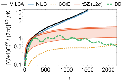
An estimate for the tSZ spectrum can be taken from Fig. 2 of Hill and Spergel (2014) or from Fig. 17 of Planck Collaboration 2015 XXII (2015). An estimate for the noise for Planck can be taken from Fig. 5 of Planck Collaboration 2015 XXII (2015), which relies on the tSZ-projected maps constructed using either. In Figure 1 we combine these estimates, together with an estimate of the total DD signal in each as per eq. (17). Note that current experimental noise is still of the same order of the best-fit tSZ templates, but future experiments such as COrE The COrE Collaboration (2011) will have noise levels well below them (we assume here a resolution of 4 arcmin and a conservative K arcmin noise level).
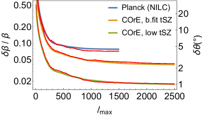
In Figure 2 we depict the achievable precision in the inferred value of the dipole by both Planck and COrE (or COrE+, PRISM André et al. (2014), PIXIE Kogut et al. (2011) or any full-sky experiment with considerably smaller noise than the tSZ spectrum: ), using such a consistency check. Since in this case the detection is only limited by , it depends directly on its amplitude. We thus consider two cases: the best fit and the lower bound amplitudes of the tSZ template as given by Fig. 17 of Planck Collaboration 2015 XXII (2015).
We also have built ideal full-sky simulations of the TT and of the -maps, and we have added the DD effect to the latter maps using eq. (7), with a value of as given by the measured dipole. We have run the estimator in eq. (16) on 300 simulations (for each case) and we plot in Figure 2 the standard deviation over the mean of the reconstructed value for , as a cross-check of eq. (15). Even for Planck the significance is estimated to be very high, at around . Note that for Planck there is almost no signal after since the noise starts increasing very rapidly while the signal slightly decreases, as can be seen from Figure 1; for COrE the situation is similar because, even if the noise is negligible, the ratio between the tSZ contamination and the DD signal increases for and thus the signal-to-noise grows slowly with for .
The extension of our estimators to the case of a generic direction of the dipole was derived to first order in eq. (6.1) of Quartin and Notari (2015b). In this case, the depends linearly on the 3 components of the dipole and by minimization it is straightforward to obtain the estimators and . The absolute uncertainty on each single component is given by the exact same estimate of Figure 2 and this can also be translated on an uncertainty on the direction angle by the simple relation , as discussed already in Amendola et al. (2011).
We have also tested in depth whether the dropped terms could produce any bias to our estimator by including them in the simulations described above. We got no discernible bias on the inferred nor any change in the scatter (as illustrated by the red curves in Figure 2). These terms can thus be safely ignored here. For completeness we give the coefficients of derived assuming and expanding eq. (1) to
| (19) |
with . Note that such tiny effects exhibit a different frequency dependence from the tSZ.
So far we have focused on the effects in eq. (II). Let us come back again to the DQ term in eq. (II), which was shown to be measurable in Kamionkowski and Knox (2003). In principle this can seen by Planck: different map-making techniques for extracting the blackbody signal have in fact different combinations of frequencies. Each map (SMICA, NILC, SEVEM and Commander, in the case of Planck Planck Collaboration 2015 IX (2015)) has weights . Following eq. (10), this leads to different effective terms for the different maps. So, when subtracting any two of such maps and a quadrupole remainder should be observed proportional to .
We stress here that such a remainder also contains a signal which allows us to make a consistency check, giving a measurement of and in the next section we will show how this can contaminate a tSZ map. The Planck Collaboration is aware of this, but they have not conducted such a check explicitly on the grounds that it would require a better understanding of the quadrupole foregrounds Planck Collaboration 2013 XXVII (2014). We can estimate the S/N of the DQ on a temperature map as .
The most straightforward estimation is to use directly a tSZ-projected map, for which by construction. For Planck we get that, according to Figure 1, we can estimate it as .
IV DD as a contamination to tSZ measurements and primordial -distortions
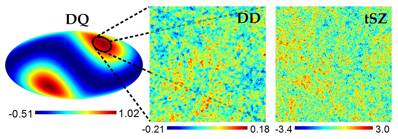
We now discuss how the DD can contaminate the standard tSZ measurements. The DD effects are maximal close to the dipole direction and its antipode. Figure 3 depicts both DD and tSZ maps in a region around the dipole direction. The DD is expected to be just a small, effect which is added to the tSZ maps. This is well below Planck’s instrumental noise, which is above the level at all scales. But it is above the expected CORE+ noise levels, and should therefore be subtracted in the future. At the level of the power spectrum the corrections are tiny, , because they mediate to zero in full-sky. We also show in the full-sky map the amplitude of the DQ in a -map. Let us also note here that such distortions, if not properly accounted for, could in principle affect also measurements of intrinsic spectral distortions. For instance PIXIE Kogut et al. (2011) should measure with a sensitivity of primordial distortions, which are expected to be produced at recombination at the level.
When measuring such distortions in the monopole it is certainly necessary to remove the monopole in eq. (II), which is , as noted in Chluba and Sunyaev (2003). However it is also relevant to remove the DD and DQ distortions. In fact, when introducing a mask, any multipole could leak into the monopole. Moreover one could be also interested in adapting future experiments like PIXIE Kogut et al. (2011) and PRISM André et al. (2014) to measure directly spectral distortions of multipoles (see Balashev et al. (2015) for the dipole). In this case a removal of DD and DQ is necessary because it is higher than the instrument sensitivity. Finally let us note that in Chluba and Sunyaev (2003) -distortions due to effects of order were also studied.
The presence of a mask enhances the leakages into the -channel. This is proportional to the asymmetry of the mask. For the power spectrum there will be an leakage on the (similar to Pereira et al. (2010)): , where is an angular average over the masked sky. Assuming a mask asymmetry of , there would be a contamination at , decreasing at higher . For small-sky experiments such as ACT ( Notari et al. (2014); Jeong et al. (2014)) the bias is larger, about at . For the maps, such a mask would also induce a leak from the DQ and a leak from the DD, which could affect the measurements of the -distortions in the monopole. We stress however that such leakages can be easily avoided by the use of a symmetric mask, as proposed in Quartin and Notari (2015b), or by subtraction using eq. (7).
V Discussion
We have shown that using a linearized formula for extracting the temperature fluctuations from intensity, one always also induces a leakage on the -maps. Such a signal is dominated by a leakage of the Dipole, the amplitude of which is and it contains in addition to the known quadrupole (DQ) and monopole of order also a signal proportional to the blackbody temperature map times a dipolar modulation of order over the whole sky, which comes from a cross-term between the Dipole and the rest of the map. Using the information from the temperature blackbody map, we are able to predict precisely the latter signal (which we called DD) at the level of the individual ’s. As we have shown the DD should be present already in Planck at about and future experiments are only limited by the degeneracy with the tSZ signal. Detecting this type of signal constitutes a consistency check of the map-making procedure. We also pointed out that the measurement performed in Planck Collaboration 2013 XXVII (2014) should have first removed the -type part of the signal, which is not carrying information independent from the CMB dipole, and then should have measured the blackbody Doppler couplings which are truly induced by a boost. Applying such a procedure will lead to a decrease in the signal-to-noise ratio in the Doppler estimator.
Vice versa, we stress that all such signals should be subtracted in order to see the tSZ signal or other physical -distortions in a clean way. We have shown that the DD signal, which spans over all angular scales, is at most between and of the tSZ signal close to the direction of our dipole (see Figure 3), and is less important in regions which are far away from it. This may not be a large contamination, but it is higher than the expected instrumental noise levels in the next-generation CMB experiments. For comparison the DQ is the largest distortion, but it only affects the mode.
Moreover such effects could contaminate measurements of intrinsic spectral distortions in the CMB: while a monopole and a DQ are known to give rise to a signal, we have pointed out that the DD gives rise to a non-negligible signal on all multipoles. Even if one focuses on measuring only monopole distortions, also the latter should be carefully subtracted in order to avoid possible leakages due to partial sky coverage.
Acknowledgments
We thank Barbara Comis for useful clarifications, and Craig Copi, Glenn Starkman, Jordi Miralda, Marcio O’Dwyer, Omar Roldan, Jim Zibin and Antony Lewis for interesting discussions. We also acknowledge important suggestions and corrections from the anonymous referees. MQ is grateful to Brazilian research agencies CNPq and FAPERJ for support and to the University of Barcelona for hospitality. AN is supported by the grants EC FPA2010-20807-C02-02, AGAUR 2009-SGR-168.
Appendix A DD in Planck maps
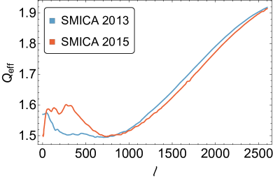
Planck maps were not built with the goal of removing the Dipolar Distortions. In fact, their CMB temperature maps do not even project out the -channel. This is probably due to the fact that the tSZ was not a large foreground and thus not removed in their different component separation techniques. This can be explicitly seen for the SMICA maps. In particular, for SMICA 2013 and 2015 we computed explicitly the sum of eq. (10) using the reported weights for all different multipoles. The result is in Figure 4. The weights were reconstructed from Planck Collaboration 2013 XII (2014) and Planck Collaboration 2015 IX (2015). Note that the result is different from zero at all scales, meaning that there is a contamination due to the -channel and thus also due to the DD. For the other map-making techniques used by Planck (NILC, SEVEM and Commander) defining an effective for different scales is not a straightforward task as they are not obtained through a simple weighted sum in harmonic space.
References
- Bennett et al. (2013) C. L. Bennett et al. (WMAP), Astrophys. J. Suppl. 208, 20 (2013), arXiv:1212.5225 [astro-ph.CO] .
- Planck Collaboration 2015 I (2015) Planck Collaboration 2015 I, (2015), arXiv:1502.01582 [astro-ph.CO] .
- André et al. (2014) P. André et al. (PRISM), JCAP 1402, 006 (2014), arXiv:1310.1554 [astro-ph.CO] .
- Kamionkowski and Knox (2003) M. Kamionkowski and L. Knox, Phys.Rev. D67, 063001 (2003), arXiv:astro-ph/0210165 [astro-ph] .
- Chluba and Sunyaev (2003) J. Chluba and R. Sunyaev, Astron.Astrophys. 424, 389 (2003), arXiv:astro-ph/0404067 [astro-ph] .
- Planck Collaboration 2013 XXVII (2014) Planck Collaboration 2013 XXVII, Astron.Astrophys. 571, A27 (2014), arXiv:1303.5087 [astro-ph.CO] .
- Planck Collaboration 2015 VIII (2015) Planck Collaboration 2015 VIII, (2015), arXiv:1502.01587 [astro-ph.CO] .
- Roldan et al. (2016) O. Roldan, A. Notari, and M. Quartin, JCAP 1606, 026 (2016), arXiv:1603.02664 [astro-ph.CO] .
- Notari and Quartin (2015) A. Notari and M. Quartin, JCAP 1506, 047 (2015), arXiv:1504.02076 [astro-ph.CO] .
- Quartin and Notari (2015a) M. Quartin and A. Notari, JCAP 1509, 050 (2015a), arXiv:1504.04897 [astro-ph.IM] .
- Planck Collaboration 2016 XLVI (2016) Planck Collaboration 2016 XLVI, (2016), arXiv:1605.02985 [astro-ph.CO] .
- Notari and Quartin (2012) A. Notari and M. Quartin, JCAP 1202, 026 (2012), arXiv:1112.1400 [astro-ph.CO] .
- Challinor and van Leeuwen (2002) A. Challinor and F. van Leeuwen, Phys.Rev. D65, 103001 (2002), arXiv:astro-ph/0112457 [astro-ph] .
- Kosowsky and Kahniashvili (2011) A. Kosowsky and T. Kahniashvili, Phys.Rev.Lett. 106, 191301 (2011), arXiv:1007.4539 [astro-ph.CO] .
- Amendola et al. (2011) L. Amendola, R. Catena, I. Masina, A. Notari, M. Quartin, and C. Quercellini, JCAP 1107, 027 (2011), arXiv:1008.1183 [astro-ph.CO] .
- Chluba (2011) J. Chluba, Mon. Not. Roy. Astron. Soc. 415, 3227 (2011), arXiv:1102.3415 [astro-ph.CO] .
- Sazonov and Sunyaev (1998) S. Y. Sazonov and R. A. Sunyaev, Astrophys. J. 508, 1 (1998), arXiv:astro-ph/9804125 [astro-ph] .
- Sunyaev and Khatri (2013) R. A. Sunyaev and R. Khatri, JCAP 1303, 012 (2013), arXiv:1302.6571 [astro-ph.CO] .
- Balashev et al. (2015) S. A. Balashev, E. E. Kholupenko, J. Chluba, A. V. Ivanchik, and D. A. Varshalovich, Astrophys. J. 810, 131 (2015), arXiv:1505.06028 [astro-ph.CO] .
- Fixsen (2009) D. J. Fixsen, Astrophys. J. 707, 916 (2009), arXiv:0911.1955 [astro-ph.CO] .
- Planck Collaboration 2015 XXII (2015) Planck Collaboration 2015 XXII, (2015), arXiv:1502.01596 [astro-ph.CO] .
- Quartin and Notari (2015b) M. Quartin and A. Notari, JCAP 1501, 008 (2015b), arXiv:1408.5792 [astro-ph.CO] .
- Van Waerbeke et al. (2014) L. Van Waerbeke, G. Hinshaw, and N. Murray, Phys. Rev. D89, 023508 (2014), arXiv:1310.5721 [astro-ph.CO] .
- Hill and Spergel (2014) J. C. Hill and D. N. Spergel, JCAP 1402, 030 (2014), arXiv:1312.4525 [astro-ph.CO] .
- Catena and Notari (2013) R. Catena and A. Notari, JCAP 1304, 028 (2013), arXiv:1210.2731 [astro-ph.CO] .
- The COrE Collaboration (2011) The COrE Collaboration (COrE), (2011), arXiv:1102.2181 [astro-ph.CO] .
- Kogut et al. (2011) A. Kogut et al., JCAP 1107, 025 (2011), arXiv:1105.2044 [astro-ph.CO] .
- Planck Collaboration 2015 IX (2015) Planck Collaboration 2015 IX, (2015), arXiv:1502.05956 [astro-ph.CO] .
- Pereira et al. (2010) T. S. Pereira, A. Yoho, M. Stuke, and G. D. Starkman, (2010), arXiv:1009.4937 [astro-ph.CO] .
- Notari et al. (2014) A. Notari, M. Quartin, and R. Catena, JCAP 1403, 019 (2014), arXiv:1304.3506 [astro-ph.CO] .
- Jeong et al. (2014) D. Jeong, J. Chluba, L. Dai, M. Kamionkowski, and X. Wang, Phys. Rev. D89, 023003 (2014), arXiv:1309.2285 [astro-ph.CO] .
- Planck Collaboration 2013 XII (2014) Planck Collaboration 2013 XII, Astron. Astrophys. 571, A12 (2014), arXiv:1303.5072 [astro-ph.CO] .