Electronic correlations in the Hubbard model on a bi-partite lattice

Abstract

In this work we study the Hubbard model on a bi-partite lattice using the coupled-cluster method (CCM). We first investigate how to implement this approach in order to reproduce the lack of magnetic order in the 1D model, as predicted by the exact Bethe-Ansatz solution. This result can only be reproduced if we include an algebraic correlation in some of the coupled-cluster model coefficients. Using the correspondence between the Heisenberg model and the Hubbard model in the large-coupling limit, we use very accurate results for the CCM applied to the Heisenberg and its generalisation, the $XXZ$ model, to determine CCM coefficients with the correct properties. Using the same approach we then study the 2D Hubbard model on a square and a honeycomb lattice, both of which can be though of as simplified models of real 2D materials. We analyse the charge and spin excitations, and show that with care we can obtain good results.

I Introduction

The Hubbard model Hubbard (1963) and its variations have been widely applied to investigate the electronic correlations of interacting electrons in low-dimensional systems. The simple form of the model not only provides an excellent test ground for bench-marking theoretical tools, but also has important applications in describing experimental data. The model has played an important role in our understanding of the high-$T_{c}$ superconductors over the last few decades, see, e.g., Ref. Hirsch (1985), and has been extensively studied using many microscopic methods, see, e.g., Refs. Avella and Mancini (2012, 2013) for recent reviews.

The Hubbard model consists of only two terms: a nearest-neighbour electron hopping term with strength $t$ and an on-site electronic repulsion with strength $U$. In two dimensions on a square lattice when half the available electronic states are filled, the on-site repulsion causes a Mott transition from a paramagnetic conductor to an antiferromagnetic insulator for any non-zero value of $U$ Hirsch (1985). However, the model on a honeycomb lattice shows a different picture: the paramagnetic state is stable for small $U$, and the Mott transition occurs at a non-zero value of the interaction $U=U_{c}$, which has a value of about $U_{c}/t\approx 4.5$ (see e.g., Ref. He and Lu (2012)). This quantum phase transition has attracted strong theoretical interests since the discovery of graphene and other two-dimensional materials such as silicene and Boron Nitride Xu et al. (2013) due to their hexagonal structures. Of course, the application of the Hubbard model to graphene and sister materials may be questioned and is a subject of ongoing debate; most theoretical studies of interaction effects in graphene employ the full long-range Coulomb interaction Kotov et al. (2012). Nevertheless, the Hubbard model with local interactions (the on-site and nearest neighbour interactions) has been used to investigate the electronic correlations in graphene such as the possible edge magnetism of narrow ribbons and formation of local magnetic moments (see references in Kotov et al. (2012)). Furthermore, there is also some theoretical discussion of possible spin-liquid phase between the metallic phase and the ordered antiferromagnetic insulating phase on a honeycomb lattice. Sorella et al Sorella et al. (2012) report, using a numerically exact Monte Carlo method, that there is little or no indication of such a phase transition to a spin liquid in clusters of 2592 atoms. Both Sorella et al and He et al He and Lu (2012) argue for a spin-liquid state below $U_{c}$, with a semi-metallic state only at $U=0$, with evidence for a first order Mott phase transition. Yang et al Yang et al. (2012) apply an effective Hamiltonian approach, and also find weak or no evidence for a quantum spin liquid. In the work of Lin et al Lin et al. (2015), a slightly modified version of the Hubbard model is studied.

One of the important methods to systematically study electronic correlations of interacting electron systems is the coupled-cluster method (CCM) Bishop (1991). The key advantages of the CCM are its avoidance of unphysical divergences in the thermodynamic limit and its ability to be taken to high accuracy through systematic inclusion of high-order correlations. The price to pay is that the method does not provide a variational bound to the ground state energy, and that the wave function is not Hermitian. Nevertheless, convergence of CCM calculation has been found to be rapid. Therefore, the CCM is the method of choice for state-of-the-art calculations for atomic and molecular systems in quantum chemistry, where it is used, amongst others, to calculate correlation energies, to an accuracy of less than one millihartree (1 mH) Bartlett and Musial (2007). The CCM has been successfully applied to a wide range of other physical systems, including problems in nuclear physics, both for finite and infinite nuclear matter, the electron gas and liquids, as well as various integrable and nonintegrable models, and various relativistic quantum field theories. In most such cases the numerical results are either the best or among the best available. A classical example is the electron gas, where the coupled cluster results for the correlation energy agree over the entire metallic density range to within less than 1 millihartree (or less than 1%) with the essentially exact Green’s function Monte Carlo results Bishop (1991). Most relevant to our present work, over the last two decades the CCM has also been successfully applied to describe quantum spin lattice systems accurately, providing some of the best numerical results for the ground state energy, the sub-lattice magnetization, and spin-wave excitation spectra (for a recent example see, e.g., Ref. Li and Bishop (2015)). In these applications, the full advantage of the systematic improvement by inclusion higher-order correlations attainable by computer algebra have revealed physical properties of the quantum phase transitions in spin systems.

The CCM shares quite a few of its roots with classic many-body techniques based on many-body perturbation theory, see Refs. Avella and Mancini (2012, 2013) for some modern examples. The result of CCM calculations look much like a resummation of the perturbation series, and indeed do not diverge where perturbation theory fails to converge. It is a pure method: normally one works directly with the full complement of quasi-particles relative to a generalised vacuum –usually called reference– state. There is a similarity with dynamical mean-field theory. The lowest order of CCM is like mean-field theory, and one can include higher order RPA-like correlations. In the standard formulation applied here it lacks the full power of the normal mean-field, which is included in the dynamical mean-field method, but including higher order correlations is much more systematic in CCM. Clearly the CCM is one of the family of cluster approximations. In its calculations all independent cluster excitations on the reference wave function are taken into account in the ket state–but not in the bra state to make the calculations practical. There is a variational formulation of the CCM, but with an independent bra and ket state variation, there is no variational upper bound for the energy, and excited states are solutions to a non-Hermitian eigenvalue problem. On the other hand, one can show that the Helmann-Feynman theorem is satisfied. It also means that we cn easily evaluate expectation values of any observable. Thus using CCM has both advantages and disadvantages relative to other many-body methods, and deserves to be studied in more detail for the Hubbard model.

There are a few CCM calculations using very simple approximations for the Hubbard model on a square lattice Roger and Hetherington (1990); Bishop et al. (1995). The nature of these calculations involves a systematic cluster truncation of the wave function; here we include higher-order correlations than in previous work, and extend the calculations to the honeycomb lattice. We take advantage of the fact that the Hubbard model reduces to a spin model in the large-$U$ limit and employ the existing CCM results for lattice spin models to obtain better numerical results for the ground-state energy and the sub-lattice magnetization. These ideas show some similarity with the work by Zheng, Paiva and collaborators Paiva et al. (2005); Zheng et al. (2005), who study the Hubbard model for large $U$ using a series expansion technique, and make use of the Heisenberg model results as well.

This paper is organized as follows. In Sec. II we introduce the Hubbard model and discuss its relation to the spin models. In Sec. III we provide a brief description of the CCM and the detail of its application to the Hubbard model for the ground state and excited states, including both the charge and spin-flip excitations. A particular high-order approximation scheme employing the earlier CCM results is introduced and applied. We also give the consistent results for the Hubbard model in the large-$U$ limit with the spin models. In the results section of Sec. IV, we summarize all the results for the 1D chain, and the 2D square and honeycomb models. We emphasize the significant improvement for a wide range of values of $U$ in the numerical results for the ground state energies and the magnetic order parameter (sub-lattice magnetisation) when the high-order correlations are included. We include a discussion of the indication of a phase transition for the honeycomb lattice. In the last section we provide a summery of our results and a discussion on the technical difference between the CCM calculations for the Hubbard and spin models. Some of the details of the CCM calculations can be found in appendix A. Since our work relies on the correspondence between the Hubbard and Heisenberg models, we discuss some pertinent details of that correspondence in appendix B.

II The Hubbard Model

We start from the Hubbard model defined on a bi-partite lattice, consisting of a hopping term with strength $t$ and an on-site potential $V$ with strength $U$ in terms of electron-creation operators $c^{\dagger}_{\boldsymbol{m}\sigma}$,

$$H = -t\sum_{\langle\boldsymbol{i}\boldsymbol{j}\rangle\sigma}\left(c_{\boldsymbol{i}\sigma}^{\dagger}c_{\boldsymbol{j}\sigma}+c_{\boldsymbol{j}\sigma}^{\dagger}c_{\boldsymbol{i}\sigma}\right)+U\sum_{\boldsymbol{m}}\left(n_{\boldsymbol{m}\uparrow}-\frac{1}{2}\right)\left(n_{\boldsymbol{m}\downarrow}-\frac{1}{2}\right)+\frac{NU}{4}$$ (1)

$$\equiv -tT+UV,$$ (2)

where the index $\boldsymbol{m}$ runs all $N$ lattice sites. The notation $\langle\boldsymbol{i}\boldsymbol{j}\rangle$ denotes a sum over nearest-neighbour sites (which are by definition on opposite sub-lattices), and we shall use indices $\boldsymbol{i}$ and $\boldsymbol{j}$ exclusively for one of the two sub-lattices, called $A$ and $B$, respectively. The spin index $\sigma=\uparrow,\downarrow$. Finally, the parameters $t$ and $U$ are the hopping and on-site interaction strengths, respectively. We subtract 1/2 from the number operators $n_{\boldsymbol{m}\sigma}=c_{\boldsymbol{m}\sigma}^{\dagger}c_{\boldsymbol{m}\sigma}$ in order for the excitations to have a maximally symmetric form.

In the large-$U/t$ limit, the Hamiltonian of Eq. (1) has been shown, after a unitary transformation, to be equivalent to the Heisenberg model in the subspace where $\langle V\rangle=0$, which is the space with exactly one electron occupying each lattice site Chao et al. (1978); MacDonald et al. (1988); Oleś (1990)

$$H=J\sum_{\langle\boldsymbol{i}\boldsymbol{j}\rangle}\left(\boldsymbol{S}_{\boldsymbol{i}}\cdot\boldsymbol{S}_{\boldsymbol{j}}-\frac{1}{4}\right),$$ (3)

where $J$ is given by

$$J=4t^{2}/U.$$ (4)

The objects $\boldsymbol{S}_{\boldsymbol{m}}$ are the spin-1/2 vector operators at lattice site $\boldsymbol{m}$. The Hamiltonian Eq. (3) can be derived using perturbation theory in the unitary transformation that links the two Hamiltonians, see Appendix B for a short discussion.

The Heisenberg model has been studied extensively by the coupled-cluster method (CCM) since the pioneering work of Ref. Roger and Hetherington (1990). These studies have also been generalised to the $XXZ$ model in Ref. Bishop et al. (1991),

$$H=J\sum_{\langle\boldsymbol{i}\boldsymbol{j}\rangle}\left(S_{\boldsymbol{i}}^{x}S_{\boldsymbol{j}}^{x}+S_{\boldsymbol{i}}^{y}S_{\boldsymbol{j}}^{y}+\Delta S_{\boldsymbol{i}}^{z}S_{\boldsymbol{j}}^{z}\right)$$ (5)

where the anisotropy parameter $\Delta$ distinguishes the various form of the $XXZ$ model ($\Delta>0$). The CCM analysis starts from the classical Ising limit ($\Delta\to\infty$) and includes quantum correlations in the ground state, which of course depend on the anisotropy. In particular, the analysis shows that the spin-spin correlations show algebraic decay as the anisotropy decreases to a critical value $\Delta=\Delta_{c}$. For example, on a square lattice at the critical anisotropy the spin-wave excitations become gapless with a value of spin-wave velocity in agreement with that of the second order spin-wave theory of Anderson Anderson (1952); Kubo (1952); Oguchi (1960) at the isotropic point $\Delta=1$; for the one-dimensional model, one finds the expected value zero for the sub-lattice magnetization at the critical anisotropy, in contrast to the divergent result from spin-wave theory Anderson (1952). There are good theoretical arguments that $\Delta_{c}$ converges to 1 as we increase the order of the CCM calculation.

In this paper, we apply a similar CCM analysis. We start from a Néel state and include quantum many-body correlations by considering correlations caused by excitations (both charge and spin) on top of this state. As expected, our results for the ground-state energies of the Hubbard model of Eq. (1) reduce to those of the spin models in the large-$U/t$ limit using corresponding CCM truncations. As we shall discuss in more detail below, this correspondence requires a very subtle incorporation of the Heisenberg model results into the Hubbard model, including the incorporation of the unitary transformation.

Therefore, for general values of $U/t$, we take the advantage of the results from the solution of the $XXZ$ model with the anisotropy as a parameter. We shall show that it makes sense to use the critical value, and directly employ the resulting algebraic two-body spin-spin correlations at the critical anisotropy in our study of the Hubbard model. Indeed, as we will demonstrate, the ground-state energies are at minimum at the critical anisotropy.

III Coupled-Cluster Method and the Super-SUB$n$ approximation

In the normal coupled-cluster method (NCCM) we describe the ground state of an interacting system as the exponential of a generalised creation operator acting on a generalised vacuum state (in a more group-theoretical setting, an extremal weight state) Bishop and Kümmel (1987); Bishop (1991),

$$|\Psi\rangle=e^{S}|\Phi_{0}\rangle.$$ (6)

The key idea of the CCM, is that we do not assume the bra state to be the Hermitian conjugate of the ket state. Effectively this corresponds to using a bi-orthogonal basis, where the dual states are not the Hermitian conjugates of the ket states. The advantage will be that all expressions are finite polynomials in the correlations, but the disadvantage can be that we no longer have a variational upper bound to the energy. We use the parametrisation

$$\langle\tilde{\Psi}|=\langle\Phi_{0}|(1+\tilde{S})e^{-S}.$$ (7)

The operators $S$ and $\tilde{S}$ are then expanded in generalised (multi-particle) creation and annihilation operators,

$$C_{I}\left|\Phi_{0}\right\rangle =0\text{ if $I>0$},$$

$$S=\sum_{I\neq 0}s_{I}C_{I}^{\dagger},\qquad\tilde{S}=\sum_{I\neq 0}\tilde{s}_{I}C_{I},$$ (8)

with many-body correlation coefficients $s_{I}$ and $\tilde{s}_{I}$ to be determined. Here we conventionally choose $C_{0}$ as the identity operator, and thus the inequality in the summations in Eq. (8) excludes a constant term.

The expansion (8) together with Eqs. (6) and (7) can give an in principle exact description for the ground state, by applying the variational principle to the energy. The ground state solution for the set of coefficients $s_{I}$ is then given by the non-linear equations obtained from the variation of the expectation value of the Hamiltonian, $\langle H\rangle=\left\langle\tilde{\Psi}\middle|H\middle|\Psi\right\rangle$, with respect to $\tilde{s}_{I}$,

$$\forall_{I>0}:\ \left\langle\Phi_{0}\right|C_{I}e^{-S}He^{S}\left|\Phi_{0}\right\rangle =0.$$ (9)

Using this equation, and the fact that the general energy expression is linear in $\tilde{s}$, we see that $\tilde{s}$ does not contribute to the ground-state energy,

$$E_{0} =\left\langle\Phi_{0}\right|e^{-S}He^{S}\left|\Phi_{0}\right\rangle.$$ (10)

The coefficients $\tilde{s}_{I}$, sometimes called bra-state coefficients, are thus not required for the evaluation of the ground state energy, but they do enter the expectation value of other observables through Eq. (7). They can determined from the linear equations, which follow from the variation of the general expression for the energy with respect to $s_{J}$,

$$\sum_{I>0}\tilde{s}_{I}\left\langle\Phi_{0}\right|C_{I}e^{-S}[H,C_{J}^{\dagger}]e^{S}\left|\Phi_{0}\right\rangle=0,$$ (11)

once we have determined the values of $s_{I}$ from Eq. (9).

Since there are only a finite–typically small–number of possible contractions, the equation (10) expresses the ground-state energy in terms of a small subset of the CCM coefficients $s_{I}$. Normally the CCM equations (9) involve all of the coefficients, due to the presence of the operators $C_{I}$. In many cases we can identify a hierarchy in these equations–that is commonly based on the number of basic (single-particle) operators that make up the operator $C_{I}^{\dagger}$. We then label successive terms in this hierarchy with an index $n$, and we denote the SUB$n$ approximation as the case where we use all the creation and annihilation operators up to level $n$ in the hierarchy. In principle we can systematically improve on these calculations by simply increasing $n$–though the complications increase rapidly with $n$.

III.1 CCM for the Hubbard model

The most comprehensive application of the coupled-cluster method to the Hubbard model can be found in Ref. Bishop et al. (1995), see also the earlier work Roger and Hetherington (1990). As is discussed in those papers, the common choice of reference state is the Néel state

$$|\Phi_{0}\rangle=\prod_{\boldsymbol{i},\boldsymbol{j}}c_{\boldsymbol{i}\uparrow}^{\dagger}c_{\boldsymbol{j}\downarrow}^{\dagger}|0\rangle,$$ (12)

i.e., an antiferromagnetic state where the $A$ sub-lattice is magnetised upwards, and the $B$ one downwards–so all nearest neighbours are in the classically optimal position of having their spins pointing in opposite directions. For this particular choice of reference state, it is easier to work with quasi-particle operators that are the single particle creation and annihilation operators relative to the Néel state (an extreme case of a Bogoliubov transformation)

$$a_{\boldsymbol{i}\uparrow} =c_{\boldsymbol{i}\uparrow}^{\dagger},\quad a_{\boldsymbol{i}\downarrow}=c_{\boldsymbol{i}\downarrow},$$

$$b_{\boldsymbol{j}\uparrow} =c_{\boldsymbol{j}\downarrow}^{\dagger},\quad b_{\boldsymbol{j}\downarrow}=c_{\boldsymbol{j}\uparrow}.$$ (13)

In terms of these new operators we have

$$H =-t\sum_{\langle\boldsymbol{i}\boldsymbol{j}\rangle}\left(b_{\boldsymbol{j}\uparrow}a_{\boldsymbol{i}\downarrow}-b_{\boldsymbol{j}\downarrow}a_{\boldsymbol{i}\uparrow}+a_{\boldsymbol{i}\downarrow}^{\dagger}b_{\boldsymbol{j}\uparrow}^{\dagger}-a_{\boldsymbol{i}\uparrow}^{\dagger}b_{\boldsymbol{j}\downarrow}^{\dagger}\right)+$$

$$-U\sum_{\boldsymbol{i}}a_{\boldsymbol{i}\downarrow}^{\dagger}a_{\boldsymbol{i}\uparrow}^{\dagger}a_{\boldsymbol{i}\uparrow}a_{\boldsymbol{i}\downarrow}-U\sum_{\boldsymbol{j}}b_{\boldsymbol{j}\downarrow}^{\dagger}b_{\boldsymbol{j}\uparrow}^{\dagger}b_{\boldsymbol{j}\uparrow}b_{\boldsymbol{j}\downarrow}+\frac{U}{2}(n_{a}+n_{b}).$$ (14)

We now expand the CCM correlations in terms of powers of the creation operators $a^{\dagger}$ and $b^{\dagger}$, the SUB$n$ expansion, as

$$S=\sum_{k=1}^{n}S_{k},\,\tilde{S}=\sum_{k=1}^{n}\tilde{S}_{k}.$$ (15)

Since the total spin projection quantum number is conserved, we always find an equal number of spin up and spin down operators in each $S_{n}$, and thus an equal number of $a$ and $b$ operators. The lowest order term takes the form

$$S_{1} =\sum_{\boldsymbol{i}\boldsymbol{j}}s_{\boldsymbol{i}\boldsymbol{j}}\left(a_{\boldsymbol{i}\uparrow}^{\dagger}b_{\boldsymbol{j}\downarrow}^{\dagger}-a_{\boldsymbol{i}\downarrow}^{\dagger}b_{\boldsymbol{j}\uparrow}^{\dagger}\right),$$ (16)

i.e., where the CCM operators $C_{I}$ are an antisymmetric combination of one $a$ and one $b$ creation operator.

It may be interesting here to comment on the choice of antisymmetry under spin exchange of the operator in Eq. (16), which is not immediately obvious from the discussion above. It is actually more restrictive than one would expect, but additional analysis shows that it is an operator that adds a spin-zero pair of quasi-particles to the Néel state. That explains why this is the correct structure: it is due to the fact that the Hamiltonian (14) is actually a quasi-particle spin $0$ operator, and the Néel state, which is the quasi-particle vacuum state, has spin zero as well. Thus any correlated state build upon this must also have this symmetry. Alternatively, this structure can be shown to be correct for the ground state due to its symmetry under exchange of $a_{i\sigma}^{\dagger}\leftrightarrow b_{j\bar{\sigma}}^{\dagger}$ (where the bar denotes a spin-flip, $\bar{\uparrow}=\downarrow$, $\bar{\downarrow}=\uparrow$) together with the anticommutation of the fermion operators.

The most general $S_{2}$ operator can be decomposed in three components,

$$S_{2} =\sum_{\boldsymbol{i}\boldsymbol{i}^{\prime}\boldsymbol{j}\boldsymbol{j}^{\prime}}\bigg{(}s_{\boldsymbol{i}\boldsymbol{i}^{\prime}\boldsymbol{j}\boldsymbol{j}^{\prime}}^{(1)}a_{\boldsymbol{i}\uparrow}^{\dagger}a_{\boldsymbol{i}^{\prime}\downarrow}^{\dagger}b_{\boldsymbol{j}\downarrow}^{\dagger}b_{\boldsymbol{j}^{\prime}\uparrow}^{\dagger}+$$

$$\qquad\quad s_{\boldsymbol{i}\boldsymbol{i}^{\prime}\boldsymbol{j}\boldsymbol{j}^{\prime}}^{(2)}a_{\boldsymbol{i}\uparrow}^{\dagger}a_{\boldsymbol{i}^{\prime}\uparrow}^{\dagger}b_{\boldsymbol{j}\downarrow}^{\dagger}b_{\boldsymbol{j}^{\prime}\downarrow}^{\dagger}+s_{\boldsymbol{i}\boldsymbol{i}^{\prime}\boldsymbol{j}\boldsymbol{j}^{\prime}}^{(3)}a_{\boldsymbol{i}\downarrow}^{\dagger}a_{\boldsymbol{i}^{\prime}\downarrow}^{\dagger}b_{\boldsymbol{j}\uparrow}^{\dagger}b_{\boldsymbol{j}^{\prime}\uparrow}^{\dagger}\bigg{)}.$$ (17)

We have a similar form for $\tilde{S}$, but now in term of annihilation operators,

$$\tilde{S}_{1}=\sum_{\boldsymbol{i}\boldsymbol{j}}\tilde{s}_{\boldsymbol{i}\boldsymbol{j}}\left(b_{\boldsymbol{j}\downarrow}a_{\boldsymbol{i}\uparrow}-b_{\boldsymbol{j}\uparrow}a_{\boldsymbol{i}\downarrow}\right),$$ (18)

and similar for $\tilde{S}_{2}$. Explicit investigation of the SUB2 truncation, retaining only $S_{1}$ and $S_{2}$, shows that the coefficients $s^{(2)}$ and $s^{(3)}$are solutions to a homogeneous linear problem, and are thus zero in the ground state . Since the ground state is translationally invariant, we find that independent of truncation the coefficients $s$ (16) are also translationally invariant, $s_{\boldsymbol{i}\boldsymbol{j}}=s_{\boldsymbol{j}-\boldsymbol{i}}\equiv s_{\boldsymbol{r}}$.

Here, and in the remainder of this paper we shall use the symbol $\boldsymbol{r}$ to denote a vector pointing from a point on the $A$ sublattice to a point on the $B$ sublattice. We shall also use the symbol $\boldsymbol{\rho}$ to denote the values of $\boldsymbol{r}$ that connect nearest neighbours. Solving the CCM equations, we find that all $s_{\boldsymbol{\rho}}$ are the same, $s_{\boldsymbol{\rho}}=s_{1}$, since the lattice symmetries assure that these parameters are direction independent in the ground state.

The exact expression for the energy in the CCM approach is given by (here $z$ is the lattice coordination number, the number of nearest neighbours of every lattice point)

$$E_{0}/N=t\sum_{\boldsymbol{\rho}}s_{\boldsymbol{\rho}}\equiv zts_{1},$$ (19)

which only depends on the value of $s_{1}$. By selecting those equations from Eq. (9) where $C_{I}$ consists of one $a$ and one $b$ annihilation operator, we find the one-body equation

$$2t\sum_{\boldsymbol{\rho}}\left(\delta_{\boldsymbol{r}\boldsymbol{\rho}}-\sum_{\boldsymbol{r}^{\prime}}s_{\boldsymbol{r}^{\prime}}s_{\boldsymbol{r}-\boldsymbol{r}^{\prime}+\boldsymbol{\rho}}\right)+2Us_{\boldsymbol{r}}+t\sum_{\boldsymbol{i}_{1}}\sum_{\boldsymbol{\rho}}\left(s_{\boldsymbol{i}_{1}\boldsymbol{i}_{2}\boldsymbol{i}_{1}+\boldsymbol{\rho},\boldsymbol{i}_{2}+\boldsymbol{r}}^{(1)}+s_{\boldsymbol{i}_{2}\boldsymbol{i}_{1}\boldsymbol{i}_{2}+\boldsymbol{r},\boldsymbol{i}_{1}+\boldsymbol{\rho}}^{(1)}\right)=0.$$ (20)

The second order coefficient $s^{(}1)$ appears in this equation due to contraction with the Hamiltonian in the evaluation of $e^{-S}He^{S}$. This equation is exact for any SUB$n$ truncation with $n\geq 2$. Similarly, the two-body equations (obtained for $C_{I}$’s consisting of two $a$ and two $b$ operators) will involve higher-order coefficients as well. This leads to an infinite hierarchy of equations, which require a closure approximation or even a truncation, in order to make the equations tractable.

III.1.1 SUB1 approximation

The simplest truncation to make is the SUB1 approximation, by which we denote a calculation where we only include the $S_{1}$ operator. It is quite illustrative to work through the derivation of these results in some detail to illustrate the methodology; for the more complicated calculations in the following sections the derivation is given in Appendix A.

From Eq. (20) we find the one-body equation

$$t\sum_{\boldsymbol{\rho}}\left(\delta_{\boldsymbol{r}\boldsymbol{\rho}}-\sum_{\boldsymbol{r}^{\prime}}s_{\boldsymbol{r}^{\prime}}s_{\boldsymbol{r}-\boldsymbol{r}^{\prime}+\boldsymbol{\rho}}\right)+Us_{\boldsymbol{r}}=0.$$ (21)

This can be solved by a sublattice Fourier transform, see, e.g., Bishop et al. (1991), by writing

$$s_{\boldsymbol{q}} =\sum_{\boldsymbol{r}}e^{i\boldsymbol{q}\cdot\boldsymbol{r}}s_{\boldsymbol{r}},$$ (22)

$$s_{\boldsymbol{r}} =\frac{1}{|\mathcal{A}|}\int_{{}_{\mathcal{A}}}e^{-i\boldsymbol{q}\cdot\boldsymbol{r}}s_{\boldsymbol{q}}\,d\boldsymbol{q},$$ (23)

and, when required (note the complex conjugate Fourier transform),

$$\tilde{s}_{\boldsymbol{r}}=\frac{1}{|\mathcal{A}|}\int_{{}_{\mathcal{A}}}e^{i\boldsymbol{q}\cdot\boldsymbol{r}}\tilde{s}_{\boldsymbol{q}}\,d\boldsymbol{q}.$$ (24)

Here $\mathcal{A}$ denotes the first Brillouin zone (FBZ) of the $B$ sub-lattice, and $|\mathcal{A}|$ is its area. Using the sublattice Fourier transform gives the equation

$$tz\left(\gamma_{\boldsymbol{q}}-\gamma_{-\boldsymbol{q}}s_{\boldsymbol{q}}^{2}\right)+Us_{\boldsymbol{q}}=0,$$ (25)

where

$$\gamma_{\boldsymbol{q}}\equiv\frac{1}{z}\sum_{\boldsymbol{\rho}}e^{i\boldsymbol{q}\cdot\boldsymbol{\rho}}.$$ (26)

On a general bi-partite lattice, $\gamma_{-\boldsymbol{q}}=\gamma_{\boldsymbol{q}}^{*}$. Equation (25) can now be solved as a quadratic equation. Choosing the physical root, one finds

$$s_{1}=\frac{1}{k}\frac{1}{|\mathcal{A}|}\int_{{}_{\mathcal{A}}}\left(1-\sqrt{1+k^{2}|\gamma_{\boldsymbol{q}}|^{2}}\right)d\boldsymbol{q},$$ (27)

where $k$ is the coordination-weighted ratio of coupling constants,

$$k=2zt/U,$$ (28)

as in Eq. (18) of Ref. Bishop et al. (1995).

III.1.2 SUB2 on-site approximation

In the SUB2 approximation, where we include also the $S_{2}$ operator, the energy equation (19) is unchanged, but we need to include the exact one-body CCM equation (20) and make an approximation to the two-body one,

$$-U\left[\left(s_{\boldsymbol{i}_{1}\boldsymbol{i}_{2}\boldsymbol{j}_{1}\boldsymbol{j}_{1}}^{(1)}+s_{\boldsymbol{j}_{1}-\boldsymbol{i}_{2}}s_{\boldsymbol{j}_{1}-\boldsymbol{i}_{1}}\right)\delta_{\boldsymbol{j}_{1}\boldsymbol{j}_{2}}+\left(s_{\boldsymbol{i}_{1}\boldsymbol{i}_{1}\boldsymbol{j}_{1}\boldsymbol{j}_{2}}^{(1)}+s_{\boldsymbol{j}_{1}-\boldsymbol{i}_{1}}s_{\boldsymbol{j}_{2}-\boldsymbol{i}_{1}}\right)\delta_{\boldsymbol{i}_{1}\boldsymbol{i}_{2}}-2s_{\boldsymbol{i}_{1}\boldsymbol{i}_{2}\boldsymbol{j}_{1}\boldsymbol{j}_{2}}^{(1)}\right]$$

$$-t\sum_{\boldsymbol{\rho}}\left[\sum_{\boldsymbol{i}_{3}}\left(s_{\boldsymbol{i}_{3}+\boldsymbol{\rho}-\boldsymbol{i}_{1}}s_{\boldsymbol{i}_{3}\boldsymbol{i}_{2}\boldsymbol{j}_{1}\boldsymbol{j}_{2}}^{(1)}+s_{\boldsymbol{i}_{3}+\boldsymbol{\rho}-\boldsymbol{i}_{2}}s_{\boldsymbol{i}_{1}\boldsymbol{i}_{3}\boldsymbol{j}_{1}\boldsymbol{j}_{2}}^{(1)}\right)+\sum_{\boldsymbol{j}_{3}}\left(s_{\boldsymbol{j}_{1}-\boldsymbol{j}_{3}+\boldsymbol{\rho}}s_{\boldsymbol{i}_{1}\boldsymbol{i}_{2}\boldsymbol{j}_{3}\boldsymbol{j}_{2}}^{(1)}+s_{\boldsymbol{j}_{2}-\boldsymbol{j}_{3}+\boldsymbol{\rho}}s_{\boldsymbol{i}_{1}\boldsymbol{i}_{2}\boldsymbol{j}_{1}\boldsymbol{j}_{3}}^{(1)}\right)\right] =0.$$ (29)

The lattice symmetries require that for the ground state $s^{(1)}$ is symmetric under interchange of the $i$ and $j$ indices. The two-body equation (29) is very hard to solve, as it contains objects with four independent indices; a simple first approximation is to choose a subset of coefficients, those with $i_{1}=i_{2}$ and $j_{1}=j_{2}$, and require those to be the only non-zero ones. In this on-site (OS) approximation, we thus have

$$s_{\boldsymbol{i}_{1}\boldsymbol{i}_{2}\boldsymbol{j}_{1}\boldsymbol{j}_{2}}^{(1)}=\delta_{\boldsymbol{i}_{1}\boldsymbol{i}_{2}}\delta_{\boldsymbol{j}_{1}\boldsymbol{j_{2}}}s_{\boldsymbol{j}_{1}-\boldsymbol{i}_{1}}^{(1)},$$ (30)

and a similar relation for the coefficients $\tilde{s}^{(1)}$.

This makes it straightforward to derive the CCM equations, see Appendix A.1 for details.

III.1.3 Super-SUB1 Approximation

As we shall show below, the solution of the truncated CCM equations in the OS approximation only gives a slight improvement on the simple SUB1 truncation. We believe that this is due to the fact that this approximation does not contain some important correlations. In other words, we may need to consider the SUB3 truncation for the Hubbard model. This may come as a surprise since for the Heisenberg model the SUB2 scheme is highly accurate. Due to the fact that we need to perform a unitary transformation to link the two models, in the Hubbard model, we can only describe similar correlations in the SUB3 approximation. This would be a very challenging calculation, and therefore we investigate an alternative closure approximation which includes the most important effects of the SUB3 truncation, but does not require a direct evaluation. We take advantage of the fact that the exact one-body equation Eq. (20) only contains $S_{1}$ and $S_{2}$ coefficients, and we take the SUB2 coefficients $s_{\boldsymbol{r}}^{(1)}$ and $\tilde{s}_{\boldsymbol{r}}^{(1)}$ from a related calculation. A natural choice would be the the CCM solution of the Heisenberg model, but as discussed before we shall use the more general spin-$1/2$ $XXZ$ model. Thus we choose $s_{\boldsymbol{r}}^{(1)}=\alpha_{\boldsymbol{r}}^{\Delta}$ and $\tilde{s}_{\boldsymbol{r}}^{(1)}=\tilde{\alpha}_{\boldsymbol{r}}^{\Delta}$, where we use $\alpha_{\boldsymbol{r}}^{\Delta}$ and $\tilde{\alpha}_{\boldsymbol{r}}^{\Delta}$ to refer to the ket and bra SUB2 coefficients for the $XXZ$ model with anisotropy factor $\Delta$ Bishop and Rosenfeld (1998). Strictly speaking, the parameter $\Delta$ should be $1$, since, as stated before, the Hubbard model goes to the $\Delta=1$ Heisenberg model in the large $U/t$ limit. We prefer to find the optimal choice of $\Delta$ for finite $U/t$. We shall show that the energy is minimal for the critical value of $\Delta$, where the CCM coefficients generate power-law decay of the correlation functions Bishop and Rosenfeld (1998). This critical behaviour is crucial in describing the one-dimensional model, and we shall argue that the critical value of $\Delta$ is the optimal choice. Explicit expressions for the CCM parameters are given in Appendix A.2.

III.1.4 Link to the Heisenberg model

If we want to exploit the link to the Heisenberg model more fully, we first need to investigate the behaviour of our results in the limit $U\rightarrow\infty.$ It is straightforward to show that in the SUB2 on-site approximation, the $s^{(1)}$ coefficients collapse to the double-flip coefficients of the SUB2-1 approximation for the $XXZ$ model at $\Delta=1$. Here one retains the full set of SUB1 coefficients and only the nearest neighbour SUB2 coefficient $s_{1}^{(1)}$. One finds that, for any bipartite lattice with coordination number $z$,

$$s_{1}^{(1)}\Bigr{|}_{U\rightarrow\infty}=\frac{1}{(2z-1)}.$$ (31)

The non-zero limit of the nearest-neighbour coefficients reflects the fact that the Néel state is not the quantum ground state in the large $U/t$ limit. This approximation also reproduces an approximation to the ground-state energy of the Heisenberg model. We find, neglecting the constant term,

$$\frac{E_{0}}{N}\Bigr{|}_{U\rightarrow\infty}=-z\frac{t^{2}}{U}\Big{(}1+s_{1}^{(1)}\Bigr{)}.$$ (32)

If we compare this to the $XXZ$-model ground-state energy in the SUB2-1 approximation,

$$\frac{E_{0}}{N}=-J\frac{z}{8}\Bigl{(}1+2\alpha_{1}^{\Delta}\Bigr{)}-J\frac{z}{8},$$ (33)

and use the relation (4), we see that these two indeed agree.

III.2 Excitation energies

There are two equivalent ways to derive the excitation energy from the CCM. The first is the bi-variational method, where we derive the excitation energies from the variations about stable equilibrium in the time-dependent variational method (sometimes called “generalised RPA” or “Harmonic Approximation”),

$$\delta\left\langle\tilde{\Psi}\middle|i\partial_{t}-H\middle|\Psi\right\rangle,=0$$ (34)

where we use the CCM states (6) and (7), but now with all the CCM coefficients depending on time. This shows the fundamental connectivity of the excitations to the ground state calculation. The disadvantage of this method is that we need to write the CCM variational functional ignoring the symmetries of the ground state, since the excited states do not share the symmetries of the ground state.

There is an alternative but completely equivalent method due to Emrich Emrich and Zabolitzky (1984); Emrich (1981a, b) based on a linearisation of the time-dependent Schrödinger equation in terms of the excitation operator $X=\sum_{J}\chi_{J}C_{J}^{\prime\dagger}$, which acts on the correlated CCM state to give the excited state $X\left|\Psi\right\rangle$. From the Schrödinger equation for this state, using the fact that $S$ and $X$ commute, we derive

$$e^{-S}He^{S}X\left|\Phi_{0}\right\rangle=EX\left|\Phi_{0}\right\rangle,$$ (35)

we can, by using projection on the states $\left\langle\Phi_{0}\right|C^{\prime}_{I}$, subtracting the ground state energy, and using Eqs. (6,7,8), obtain the equations

$$\sum_{J}\left\langle\Phi_{0}\right|C_{I}^{\prime}e^{-S}[H,C_{J}^{\prime\dagger}]e^{S}\left|\Phi_{0}\right\rangle\chi_{J} =\omega\chi_{I},$$ (36)

This is a linear eigenvalue problem for the excitation energies $\omega$. One should keep in mind that in principle we are not guaranteed that the eigenvalues are real, since CCM does not guarantee hermiticity–the fact that all physical eigenvalues have to be real can be used an important check on the quality of the approximations made to obtain the results. The reason we label the operators $C$ by a prime is that we usually consider creation operators that do not have the symmetry of the ground state, and they are thus not the same as the operators $C$ that occur in the ground-state calculation.

In this paper we shall consider both charge excitations and spin-flip modes. We shall label the energy spectrum by the “good quantum numbers”, particle number $n$ and total quasi-particle spin $S_{\text{tot}}$, and spin projection $S_{\text{tot}z}$

$$E=E(n,S_{\text{tot}},S_{\text{tot}z}).$$ (37)

III.2.1 Charge excitations

We first look at single-particle and single-hole (charge) excitations. We associate the operators $X^{h,p}$ with coefficients $\chi_{I}^{h,p}$, where the set of indices $\{I\}$ differs for electrons/particles ($p$) and holes ($h$). In the simplest approximation, we consider excitation operators that contain only a single quasi-particle operator,

$$X^{h} =\sum_{\boldsymbol{i}}^{N/2}\chi_{\boldsymbol{i}}^{h}\,a_{\boldsymbol{i}\uparrow}^{\dagger},$$ (38)

$$X^{p} =\sum_{\boldsymbol{i}}^{N/2}\chi_{\boldsymbol{i}}^{p}\,a_{\boldsymbol{i}\downarrow}^{\dagger},$$ (39)

The energy or both particle and hole states are identical, and are the same for the SUB1 and the super-SUB1 approximations. They are given by

$$\omega_{\boldsymbol{q}}^{c}=-zts_{\boldsymbol{q}}\,\gamma_{-\boldsymbol{q}}+\frac{1}{2}U.$$ (40)

By substituting Eq. (67) into Eq. (40) we get the explicit form

$$\omega_{\boldsymbol{q}}^{c}=\frac{U}{2}\sqrt{1+k^{2}(1+\alpha_{1}^{\Delta})\,|\gamma_{\boldsymbol{q}}|^{2}}.$$ (41)

Again, at $\alpha_{1}^{\Delta}=0$ the super-SUB1 solution collapses to the SUB1 one.

III.2.2 Spin-flip excitations

The spin-excitation equation is obtained within the NCCM framework by using spin-flip operators for $C_{J}^{\prime\dagger}$. These generate states with a non-zero total spin $S_{\text{tot}}$ without affecting the total number of electrons,

$$X^{s}=\sum_{I}\chi_{I}^{s}\,\hat{C}_{I}^{\prime\dagger}.$$ (42)

The spin-excitation energy is the difference between the energy of the spin-flipped state, $E(N,S_{\text{tot}}\neq 0)$, and the ground-state energy $E_{0}(N,S_{\text{tot}}=0)$ at half filling,

$$\omega^{s}=E(N,S_{\text{tot}},S_{\text{tot}z})-E_{0}(N,0,0).$$ (43)

In this paper we shall consider the case of pure spin-flip,

$$\langle\Phi_{0}|a_{\boldsymbol{i}^{\prime}\downarrow}a_{\boldsymbol{i}\uparrow}e^{-S}[H,X^{s}]e^{S}|\varphi_{0}\rangle=\omega^{s}\chi_{\boldsymbol{i},\boldsymbol{i}^{\prime}}^{s},$$ (44)

where

$$\omega^{s}=E(N,1,-1)-E_{0}(N,0,0),$$ (45)

and the single spin-flip operator is defined as

$$X^{s} =\sum_{\boldsymbol{i}_{1},\boldsymbol{i}_{2}}^{N/2}\chi_{\boldsymbol{i}_{1},\boldsymbol{i}_{2}}^{s}\,a_{\boldsymbol{i}_{1}\uparrow}^{\dagger}a_{\boldsymbol{i}_{2}\downarrow}^{\dagger},$$ (46)

where $\chi_{\boldsymbol{i}_{1},\boldsymbol{i})2}$ are the excitation correlation coefficients, which as the indices show both act on the A sublattice. The operator $X^{S}$ removes a spin-up electron from the A sublattice, and adds an electron with the opposite spin projection elsewhere on the same lattice.

The spin-flip equation in both SUB1 and super-SUB1 approximations reduces to

$$-t\,\sum_{\langle\boldsymbol{i},\boldsymbol{j}\rangle}^{N/2}\Bigl{(}\chi_{\boldsymbol{i,}\boldsymbol{i}_{1}}^{s}\,s_{\boldsymbol{i}_{2},\boldsymbol{j}}+\chi_{\boldsymbol{i}_{2},\boldsymbol{i}}^{s}\,s_{\boldsymbol{i}_{1},\boldsymbol{j}}\Bigr{)}+U\,\chi_{\boldsymbol{i}_{1},\boldsymbol{i}_{2}}^{s}\Bigl{(}1-\delta_{\boldsymbol{i}_{1},\boldsymbol{i}_{2}}\Bigr{)}=\omega^{s}\,\chi_{\boldsymbol{i}_{1},\boldsymbol{i}_{2}}^{s}.$$ (47)

As is common, see e.g. Ref. Bishop et al. (1991), a sublattice plane wave solution is considered for the solution of Eq. (47),

$$\chi_{\boldsymbol{i},\boldsymbol{i}^{\prime}}^{s}=\frac{1}{|\mathcal{A}|^{2}}\int d\boldsymbol{q}\int d\boldsymbol{q^{\prime}}\,\chi_{\boldsymbol{q},\boldsymbol{q}^{\prime}}^{s}\,e^{-\text{i}\boldsymbol{q}\cdot\boldsymbol{i}}\,e^{-\text{i}\boldsymbol{q}^{\prime}\cdot\boldsymbol{i}^{\prime}},$$ (48)

where both $\boldsymbol{q}$ and $\boldsymbol{q}^{\prime}$ are defined on the Brillouin zone of the A sublattice. This leads to the simple eigenvalue problem

$$\left(\omega_{\boldsymbol{q}_{1}}^{c}/t+\omega_{\boldsymbol{q}_{2}}^{c}/t\right)\chi_{\boldsymbol{q}_{1}\boldsymbol{q}_{2}}-\frac{U}{t}\frac{2}{N}\sum_{\boldsymbol{q}_{1}^{\prime}\boldsymbol{q}_{2}^{\prime}}\delta_{\boldsymbol{q}_{1}^{\prime}+\boldsymbol{q}_{2}^{\prime},\boldsymbol{q}_{1}+\boldsymbol{q}_{2}}^{\text{latt}}\chi_{\boldsymbol{q}_{1}^{\prime}\boldsymbol{q}_{2}^{\prime}}=\omega^{s}/t\,\chi_{\boldsymbol{q}_{1}\boldsymbol{q}_{2}},$$ (49)

where $\omega_{\boldsymbol{q}}^{c}$ is the energy of the charge excitations (40), effectively the single particle-contribution to the excitation energy, and the interaction term contains the lattice delta $\delta^{\text{latt}}$, which has “Umklapp” equivalence, i.e., vectors are taken equal after being transformed back into the first Brillouin zone. It is thus natural to label these excitations by their total momentum $\boldsymbol{Q}=\boldsymbol{q}_{1}+\boldsymbol{q}_{2}$, transformed back into the FBZ. Since the diagonal matrix $\left(\omega_{\boldsymbol{q}_{1}}^{c}+\omega_{\boldsymbol{q}_{2}}^{c}\right)\delta_{\boldsymbol{q}_{1}\boldsymbol{q}_{1}^{\prime}}\delta_{\boldsymbol{q}_{2}\boldsymbol{q}_{2}^{\prime}}$ does not commute with the matrix $\delta_{\boldsymbol{q}_{1}^{\prime}+\boldsymbol{q}_{2}^{\prime},\boldsymbol{q}_{1}+\boldsymbol{q}_{2}}^{\text{latt}}$, this is actually an interesting and non-trivial eigenvalue problem.

Fortunately, it is simple to analyse the large $U/t$ limit: Here $\omega^{c}/t\rightarrow\frac{1}{2}U/t$, so the first term in (49) becomes $U/t$ times the identity matrix, and now commutes with the second term. The second term has a block-diagonal form: each block (for fixed $\boldsymbol{Q}$) in the matrix has dimension $N/2$ by $N/2$. Within each block this matrix has one eigenvalue $-U/t$ and the remaining $N/2-1$ eigenvalues are $0$. Within these blocks the eigenvalues $\omega^{s}/t$ are thus $N/2-1$ times $U/t$, and one eigenvalue zero, for every value of $\boldsymbol{Q}$. This zero eigenvalue has eigenvector $\sqrt{\frac{2}{N}}(1,1,\ldots,1)$. Such a fully-delocalised eigenstate in Fourier space corresponds to a local state in coordinate space ($\boldsymbol{i}_{1}=\boldsymbol{i}_{2}$ in Eq. (47)), which is the usual local (on-site) spin flip excitation that describes the magnon states in the Heisenberg model.

Following a similar analysis for the $S_{\text{tot}}=1,S_{\text{tot}z}=1$ state we find exactly the same excitation spectrum. The third member of the multiplet, the states with $S_{\text{tot}}=1$ and $S_{\text{tot}z}=0$ have a noninteracting spectrum, $\omega=\omega_{\boldsymbol{q}_{1}}^{c}+\omega_{\boldsymbol{q}_{2}}^{c}$, and are thus of little interest at this level of approximation.

III.2.3 Link to the Heisenberg model and improved spectra

The result has a clear link to the Heisenberg model. At large $U/t$ we find a clear separation between a single state a low energy, and a continuum at much higher energy. The low energy state is in the space with $\langle V\rangle=0$, which is isomorphic to the space of spin states MacDonald et al. (1988). This can thus be interpreted as the spin-wave excitation of the Heisenberg model. The high energy continuum states have multiple occupation on a single site, and thus occur at a much higher energy.

In the large $U/t$ limit we can again use a perturbation argument to find the energy of the lowest state; we find that the energy of the lowest-energy local spin-flip excitations goes like

$$\omega^{s}/t\quad \underset{U/t\rightarrow\infty}{\rightarrow}U/t\frac{1}{2}k^{2}(1+\alpha_{1}^{\Delta})\,\frac{2}{N}\sum_{\boldsymbol{q}}|\gamma_{\boldsymbol{q}}|^{2}$$

$$=\frac{t}{U}2z(1+\alpha_{1}^{\Delta}),$$ (50)

which is a flat (momentum-independent) energy spectrum with a magnitude equal to the amplitude of the spin-wave spectrum as found in the CCM approximation for the Heisenberg model Bishop et al. (1991).

As discussed in appendix B, a more detailed analysis shows that the only difference between this answer and the spin-wave spectrum found in Ref. Bishop et al. (1991) is the additional term proportional to $s^{(1)}$ in the excitation energy in this reference. Using the fact that the correspondence between Hubbard and Heisenberg models involves both a unitary transformation and a perturbation expansion, the simplest way to take the additional contribution into account is just to add this term into our equation, in the spirit of the super-SUB1 approximation for the ground state. Thus, in coordinate space, we have to solve

$$-\,\sum_{\langle\boldsymbol{i},\boldsymbol{j}\rangle}^{N/2}\Bigl{(}\chi_{\boldsymbol{i,}\boldsymbol{i}_{1}}^{s}\,s_{\boldsymbol{i}_{2},\boldsymbol{j}}+\chi_{\boldsymbol{i}_{2},\boldsymbol{i}}^{s}\,s_{\boldsymbol{i}_{1},\boldsymbol{j}}\Bigr{)}-2\frac{t}{U}\sum_{\boldsymbol{r},\boldsymbol{\rho}}s^{(1)}_{\boldsymbol{r}}\chi_{{\boldsymbol{i}}_{1},{\boldsymbol{i}}_{1}}\delta_{\boldsymbol{i}_{1},\boldsymbol{r}-\boldsymbol{\rho}}+\frac{U}{t}\,\chi_{\boldsymbol{i}_{1},\boldsymbol{i}_{2}}^{s}\Bigl{(}1-\delta_{\boldsymbol{i}_{1},\boldsymbol{i}_{2}}\Bigr{)}=\frac{\omega^{s}}{t}\,\chi_{\boldsymbol{i}_{1},\boldsymbol{i}_{2}}^{s}.$$ (51)

As discussed in more detail in appendix B, as an expansion to first order in $t/U$ this expression is strictly speaking only valid for small $t/U$. It seems a reasonable approximation for intermediate $U$, but it definitely fails when $U$ is close to zero. As we shall see later, one of the issues with this approximation is that the excitation energies go below zero for small $U$.

The effect of this additional term is most easily written in Fourier space, where the only modification to the results above is an additional $\boldsymbol{Q}$-dependent shift $-2z(t^{2}/U)s^{(1)}(\boldsymbol{Q})\gamma(\boldsymbol{Q})$ of the energy of each mode. In the large $U$ limit, the low-energy spectrum thus collapses to

$$\omega^{s}/t=\frac{t}{U}2z\left(1+\alpha_{1}^{\Delta}-\alpha_{\boldsymbol{Q}}^{\Delta}\gamma(\boldsymbol{Q})\right)$$

which agrees with the known result for the Heisenberg model Bishop et al. (1991).

IV Results

IV.1 Ground state and sublattice magnetisation

We first look at the ground state energy and the magnetic order parameter (the sub-lattice magnetisation) for the Hubbard model. We start with the exactly solvable one-dimensional model. We compare the exact result to the super-SUB1 calculations, for the critical value of $\Delta$ ($\Delta_{c}\approx 0.372755$ in 1 dimension), the SUB2-OS approximation and the mean-field results in Figs. 1. The calculation for the critical $\Delta$ gives the lowest energy results. These are actually below the exact results for all values of $U/t$, but the difference is larger for small $U/t$. For the super-SUB1 calculation for the critical value of $\Delta$, we find the correct value of zero for the sub-lattice magnetisation. The energy does not converge to the exact value for $U/t\rightarrow\infty$, that would require $\Delta=1$. On the other hand, both the mean-field and SUB2-OS approximations converge to the exact result for the energy and sub-lattice magnetisation in the limit $U/t\downarrow 0$, but they produce poor results for the ground-state energy and the order parameter for even moderate values of $U/t$. The fact that the magnetisation is described correctly is a simple effect of the algebraic nature of the correlations for $\Delta=\Delta_{c}$, and gives us substantial confidence in applying the same approximations for 2D models. Henceforth we shall only look at the critical value of $\Delta$.

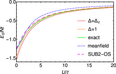
(a)

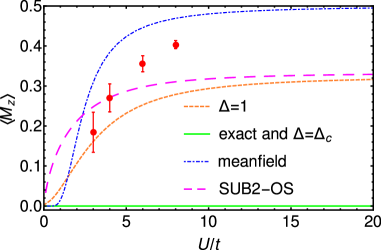
(b)

Figure 1: Ground state energy and magnetic order parameter of the 1D Hubbard model in the super-SUB1 approximation for $\Delta=\Delta_{c}$ and $\Delta=1$ compared to the exact result. We also show the results of mean-field theory and the CCM SUB2-OS approximation. The orange points (with error bars) show the Monte Carlo data from Ref. Yokoyama and Shiba (1987).

Our results for the 2D models are shown in Figs. 2 and 3. The ground state energy in the super-SUB1 approximation shows only a weak dependence on $\Delta$, which is why we only show the critical value results. The values of $\Delta_{c}$ ($0.7985$ for the square and $0.709826$ for the hexagonal lattice ) are rather close to $1$, so that in those figures we only probe a small range of parameters, which explains the similarity of the energies. Again, using $\Delta=\Delta_{c}$ gives the lowest ground state energy, and leads to a substantial reduction in the sub-lattice magnetisation for large $U/t$ which is likely to be relevant and correct, as in the 1D case. Note that the point where the magnetisaton goes through zero, is well outside the range of validity of the super-SUB1 approximation.

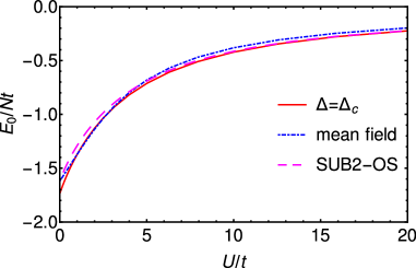
(a)

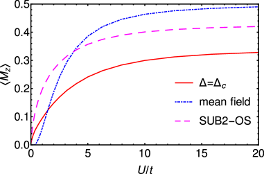
(b)

Figure 2: Ground state energy and magnetic order parameter for the 2D Hubbard model on a square lattice in the super-SUB1 approximation for $\Delta=\Delta_{c}$ compared to mean field theory and the SUB2-OS calculation.

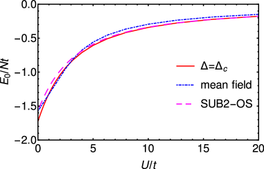
(a) The ground state energy.

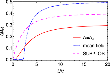
(b) The sub-lattice magnetisation.

Figure 3: Ground state energy and magnetic order parameter for the 2D Hubbard model on a honeycomb lattice in the super-SUB1 approximation for $\Delta=\Delta_{c}$ compared to mean field theory and the SUB2-OS calculation.

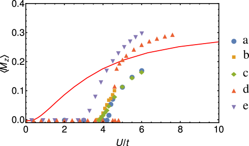
Figure 4: Comparison of our results (dashed and dotted line) to results presented in the literature: circles (a) Ref. Meng et al. (2010), squares (b) Ref. Sorella et al. (2012), lozenges (c) Ref. Assaad and Herbut (2013) (for a small magnetic field, the case $h_{0}=1$), triangles up (d) Ref. He and Lu (2012), and triangles down (e) from Ref. Chen et al. (2014). All results are scaled so that complete sub-lattice magnetisation corresponds to a value of $\langle M_{z}\rangle=1/2$. (See Fig. 3b for details of our work).

When we compare our results for the most sensitive parameter, the sub-lattice magnetisation, to some recent results in the literature, see Fig. 4, we note first of all the similarity between the literature results. The results from Ref. Chen et al. (2014) are still subject to substantial finite size corrections; and the results from Ref. Chen et al. (2014) agree on the transition point, but not on the nature of the transition and the size of the magnetisation above the transition point. In the area where we can rely on our results, which we estimate to be $U/t\gtrsim 6-8$, we find values of the magnetisation entirely consistent with the literature.

IV.2 Excited states

We now apply the method for excited states discussed in Secs. III.2.1 and III.2.2 to the Hubbard model. We label the high symmetry points in the first Brillouin zone as in Figs. 5.

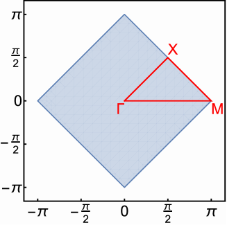
(a) square lattice.

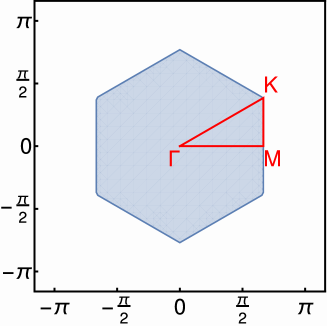
(b) honeycomb lattice.

Figure 5: The paths within the first Brillouin zone used in the presentation of excitation energies in the remainder of this paper.

IV.2.1 Charge excitations

The charge excitations, within the approximation made here, are rather similar to earlier results Roger and Hetherington (1990); Bishop et al. (1995), and thus also to those obtained with the mean-field method. The spectra show a large energy gap at large values of $U/t$: Since such excitations are suppressed in that limit, they scale as $U/t$. In Fig. 6 one can see an example of the results. In the square lattice the frequency is constant along the boundary of the first Brillouin zone (here represented as the line $M-X$) with a value of $U/2$. In the honeycomb lattice we see the dip around the $K$ point, which disappears as $U/t$ increases.

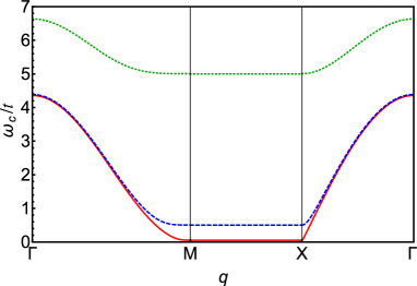
(a) Square lattice.

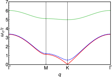
(b) Honeycomb lattice.

Figure 6: Charge excitations in the 2D Hubbard model for $U/t=0.1$ (solid red), $U/t=1$ (dashed blue) and $U/t=10$ (dotted green) for calculations in the super-SUB1 approximation.

IV.2.2 Spin-flip excitations

In the 1D case the spin-flip spectra can be calculated by solving the relevant eigenvalue problem on a lattice in $q$ space. These show a striking similarity to the pictures for two-magnon excitations in gapped 1D antiferromagnetic systems developed by Barnes Barnes (2003). This is due to the great similarity in the mathematical structure of the problems, but the physics is very different! Our results are for what is essentially a non-local single magnon excitation in the Hubbard model. The bound state at the bottom of the spectrum corresponds to the local single magnon excitation in the Hubbard model (in the large $U/t$ limit). As we can see the description of the magnon mode is not completely satisfactory; even though the continuum moves far away in this limit, the single bound state has a constant energy $\frac{t^{2}}{U}2z(1+\alpha_{1}^{\Delta})$, as specified by Eq. (50). On rather general grounds we do expect a gapless magnon in this limit Peres et al. (2004); without the Heisenberg corrections our result is only equal to the amplitude of the magnon spectrum for the Heisenberg model.

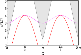
(a) $U/t=2.5$

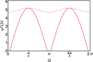
(b) $U/t=5$

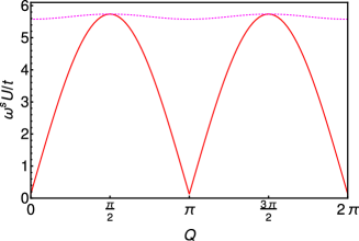
(c) $U/t=10$

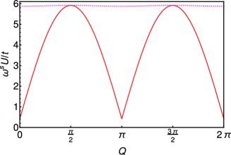
(d) $U/t=20$

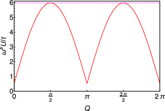
(e) $U/t=100$

Figure 7: The spin-excitation spectrum for $S_{z}=1$ in the 1D Hubbard model for several values of $U/t$. In each case we show the uncorrected approximation (dotted magenta line) and the Heisenberg corrected results for $\Delta=\Delta_{c}$ (red solid line). The grey area is the continuum of states visible for small $U/t$.

We have already discussed how we can correct for some of these shortcomings when we analyse the Heisenberg model; if we add the corrections discussed in Sec. III.2.3 we should get much better answers for small $t/U$. As we can see in Fig. 7, this is indeed the case. These corrections give a sensible magnon spectrum up to $U/t\simeq 5-10$, after which things break down. Interestingly, this is also roughly the range of parameters where the separation between continuum and bound state becomes comparable to the bound state energy.

Clearly in applying the super-SUB1 approximation, which is designed to improve results at large $U/t$, we pay a price at smaller values of $U/t$. As can be seen in Fig. 1a, we find a slight overbinding for large $U/t$, but this becomes a large effect for small $U/t$. The exact solution is bracketed between the $\Delta=1$ and the $\Delta=\Delta_{c}$ results down to $U/t\approx 2$, suggesting that the approximation we make gives a substantial improvement when we take $U/t$ above that value.

Since the structure of the approximation schemes is so similar, even though the results for the magnetisation looks rather different, it seems reasonable to assume that we obtain reliable results for the 2D problems for similar values of $U/t$, maybe slightly large to be on the conservative side. We first look at the square lattice, Fig. 8. As in the 1D model we see a continuum, and a bound state that merges with the continuum for small $U/t$. The continuum is flat at the lower end of the spectrum–actually since this caused by the combination of states at the edge of the Brillouin zone, the energy is exactly $U/t$. If we compare to the series expansion results from Ref. Zheng et al. (2005), who seem to have taken a similar approach to incorporating the Heisenberg model, we see that our results are very close to theirs–the difference is however larger than the quoted error-bars. Also, our spectrum is substantially flatter on the zone boundary between M and X; this can be traced to the flatness of the charge excitation spectrum in the CCM approximation: the series expansion has more structure on that boundary. It may well be that if we include higher order operators in the charge-state caclculations this result would improve substantially.

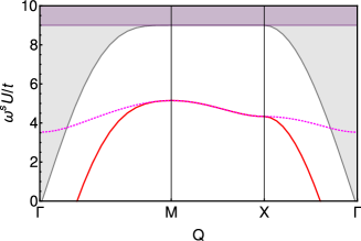
(a) $U/t=3$

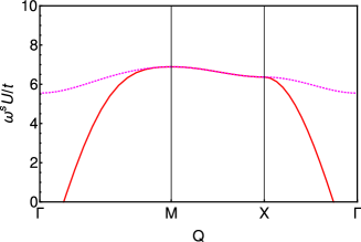
(b) $U/t=5$

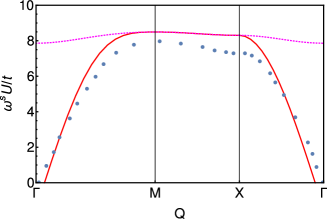
(c) $U/t=10$

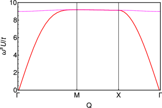
(d) $U/t=20$

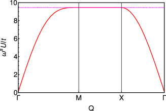
(e) $U/t=100$

Figure 8: The spin-excitation spectrum for $S_{z}=1$ for the 2D Hubbard model on the square lattice for several values of $U/t$. In each case we show the uncorrected approximation (dotted magenta line) and the Heisenberg corrected results for $\Delta=\Delta_{c}$ (red solid line). The grey area is the continuum of states visible for small $U/t$. The data points for $U/t=10$ are from the series expansion of Ref. Zheng et al. (2005) for $U/t=10.5$. We have suppressed the error bars on the series expansion results.

If we do the same thing for the model on the honeycomb lattice, Fig. 9, we see a slightly different behaviour. There still is a continuum and a bound state, but the continuum band now has structure. Once again, we see that the bound state converges to zero for large $U/t$. If we compare to the series expansion results from Ref. Paiva et al. (2005), we see that our results are very close to theirs–the error bars on the series expansion are substantial. There may be a bit more structure in the series expansion results, but we are not convinced all of this structure is real–it is not mirrored in the behaviour of the charge excitations.

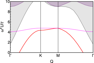
(a) $U/t=3$

(b) $U/t=5$

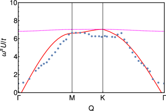
(c) $U/t=10$

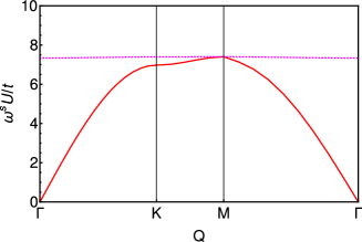
(d) $U/t=20$

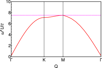
(e) $U/t=100$

Figure 9: The spin-excitation spectrum for $S_{z}=1$ for the 2D Hubbard model on the honeycomb lattice for several values of $U/t$. In each case we show the uncorrected approximation (dotted magenta line) and the Heisenberg corrected results for $\Delta=\Delta_{c}$ (red solid line). The grey area is the continuum of states visible for small $U/t$. The data points for $U/t=10$ are from the series expansion of Ref. Paiva et al. (2005) for the same value of $U/t$. We have suppressed the substantial error bars on the series expansion results.

V Outlook and Conclusions

In this paper we have investigated the ground and excitation state properties of Hubbard models in one and two-dimensions using the CCM, in similar fashion as earlier CCM analysis for the spin models. As expected, the analysis for the Hubbard models is much more involved than those of the spin models due to inclusion of the charge fluctuations, in addition to the spin fluctuations. Even though there is a close parallel between Hubbard and Heisenberg models for large $U/t$, we have concluded that the SUB2 scheme for the ground states of the spin models corresponds to the SUB3 scheme in the Hubbard model. Similar conclusion can also be drawn for the CCM analysis for the spin-flip excitations.

For efficiency purpose, we have directly employed the results of the two-body spin-spin correlations from our earlier calculations of the spin $XXZ$ model with the critical anisotropy in our evaluation of the ground state of the Hubbard models, avoiding explicit analysis of the complex SUB3 scheme, and have obtained reasonably good numerical results for the ground-state energies, the sub-lattice magnetization, and the charge excitation spectra for wide range values of the on-site interaction parameter $U/t$, when comparing with the corresponding results by numerical Monte Carlo methods. In the large-$U/t$ limit, our results reduce to those of the spin models as expected.

For the spin-flip excitation states, however, we do not obtain the corresponding gapless spin-wave spectrum as we would expect in the large-$U/t$ limit. Instead, we have obtained gapped spectra which becomes flat in the large-$U/t$ limit. We have concluded that this problem of gapped spectra can be solved by inclusion of the higher-order correlations in the excitation operators in a similar way as for the ground state, again due to the presence of charge fluctuations in the Hubbard models. More specifically, we need to consider mode-mode couplings as mentioned in Sec. IV.2.2. We have only dealt with this problem for large $U$; nevertheless our results for the spin-flip excitation states show well-defined bound states below a continuum for large values of $U/t$, with an the amplitude equal to the corresponding spin-wave velocity. The approximation breaks down as the energy of this bound state drops below the ground state near the $\Gamma$ point as $U/t$ decreases. We expect that this effect disappears when higher-order correlations in the excitation operator are included and we hope to report results in the near future.

It is also interesting to apply the extended CCM (ECCM) analysis to the Hubbard model since the lowest approximation of the ECCM will reproduce the mean-field results, to investigate in particular the properties of the metal-insulator transition for the honeycomb lattice model. We are also planning to extend our analysis to alternative models with many interesting phase structures. The Kitaev-Heisenberg model Kitaev (2006) has been generalised to a Hubbard-type model in optical lattices Duan et al. (2003) and studied in detail by Hassan and collaborators Hassan et al. (2013); Faye et al. (2014). The reason for the interest is the potential for realising an algebraic spin liquid. The only modification we need to make to to the Hubbard model is to make the hopping term spin dependent, which could be, in principle, implemented as a straightforward extension to the work reported here.

Appendix A Detailed derivation of CCM equations

A.1 SUB2 on-site approximation

The one- and two-body CCM equations now become much simpler, and we find

$$tz\left(\gamma_{\boldsymbol{q}}\left(1+s_{1}^{(1)}\right)-\gamma_{-\boldsymbol{q}}s_{\boldsymbol{q}}^{2}\right)+Us_{\boldsymbol{q}} = 0,$$ (52)

$$-U2\left[\left(s_{\boldsymbol{j}_{1}-\boldsymbol{i}_{1}}\right)^{2}\right]-4t\left(\sum_{\boldsymbol{\rho}}s_{\boldsymbol{\rho}}\right)s_{\boldsymbol{j}_{1}-\boldsymbol{i}_{1}}^{(1)} =0\implies$$

$$s_{\boldsymbol{r}}^{(1)} =-\frac{1}{k}\frac{1}{s_{1}}s_{\boldsymbol{r}}^{2},$$ (53)

where we solve for $s^{(1)}$.

We can also derive a similar set of equations for the coefficients in $\tilde{S}$ which are needed to evaluate expectation values, which we shall refer to as the one- and two-body bra-state equations,

$$k\gamma_{-\boldsymbol{q}}(1-2s_{\boldsymbol{q}}\tilde{s}_{\boldsymbol{q}})+2\tilde{s}_{\boldsymbol{q}}-2k\gamma_{-\boldsymbol{q}}\sum_{\boldsymbol{r}}\tilde{s}_{\boldsymbol{r}}^{(1)}s_{\boldsymbol{r}}^{(1)}-4\sum_{\boldsymbol{r}}e^{-i\boldsymbol{q}\cdot\boldsymbol{r}}s_{\boldsymbol{r}}\tilde{s}_{\boldsymbol{r}}^{(1)} = 0,$$ (54)

$$k\tilde{s}_{1}\frac{1}{z}\sum_{\boldsymbol{\rho}}\delta_{\boldsymbol{r},\boldsymbol{\rho}}-2ks_{1}\tilde{s}_{\boldsymbol{r}}^{(1)} = 0\implies$$

$$\tilde{s}_{\boldsymbol{r}}^{(1)} = \frac{\tilde{s}_{1}}{2zs_{1}}\delta_{|\boldsymbol{r}|,1}.$$ (55)

The remaining coefficients can be solved easily; we find

$$s_{\boldsymbol{q}}=\frac{1}{k\gamma_{-\boldsymbol{q}}}\left(1-\sqrt{1+k^{2}|\gamma_{\boldsymbol{q}}|^{2}\left[1-s_{1}/k\right]}\right),$$ (56)

together with a self-consistency condition for $s_{1}$,

$$s_{1} = \frac{1}{|\mathcal{A}|}\int_{\mathcal{A}}d\boldsymbol{q}\,\gamma_{-\boldsymbol{q}}s_{\boldsymbol{q}}$$ (57)

$$= \frac{1}{k|\mathcal{A}|}\int_{\mathcal{A}}d\boldsymbol{q}\,\left(1-\sqrt{1+k^{2}|\gamma_{\boldsymbol{q}}|^{2}\left[1-s_{1}/k\right]}\right)\,.$$

For the bra-state coefficients we have

$$\tilde{s}_{\boldsymbol{q}} = -\frac{\gamma_{-\boldsymbol{q}}}{2\sqrt{1+k^{2}|\gamma_{\boldsymbol{q}}|^{2}\left[1-s_{1}/k\right]}}\left(k-\tilde{s}_{1}\right),$$ (58)

where the value of $\tilde{s}_{1}$ can be evaluated directly,

$$\tilde{s}_{1} =\frac{1}{|\mathcal{A}|}\int_{\mathcal{A}}d\boldsymbol{q}\,\gamma_{\boldsymbol{q}}\tilde{s}_{\boldsymbol{q}}=-\frac{kI_{1}}{1-I_{1}},$$ (59)

$$I_{1} =\frac{1}{|\mathcal{A}|}\int_{\mathcal{A}}d\boldsymbol{q}\frac{|\gamma_{\boldsymbol{q}}|^{2}}{2\sqrt{1+k^{2}|\gamma_{\boldsymbol{q}}|^{2}\left[1-s_{1}/k\right]}}.$$ (60)

The order parameter for the problem is the “sub-lattice magnetisation”, the average $z$-component of the magnetisation in one of the sub-lattices (the total magnetisation is zero), $M_{z}=\frac{2}{N}\sum_{\boldsymbol{i}}S^{z}_{\boldsymbol{i}}$. We use the fact that the expectation value of an operator $O$ in the CCM approximation is given by

$$\langle O\rangle=\left\langle\tilde{\Psi}\middle|O\middle|\Psi\right\rangle=\left\langle\Phi_{0}\middle|(1+\tilde{S})e^{-S}Oe^{S}\middle|\Phi_{0}\right\rangle.$$ (61)

In the SUB1 approximation we find the simple expression

$$\langle M_{z}\rangle_{B}=\frac{1}{2}\left(1-2\frac{1}{|\mathcal{A}|}\int_{\mathcal{A}}d\boldsymbol{q}\,s_{\boldsymbol{q}}\tilde{s}_{\boldsymbol{q}}+\frac{1}{k}\tilde{s}_{1}\right).$$ (62)

A.2 Super-SUB1 Approxmation

Using the sublattice Fourier-transform, we can write the one-body equation as (with $s_{\boldsymbol{\rho}}^{(1)}\equiv s_{1}^{(1)}$ using the lattice symmetry)

$$t\left(\gamma_{\boldsymbol{q}}-\,\gamma_{-\boldsymbol{q}}\,s_{\boldsymbol{q}}^{2}+s_{1}^{(1)}\gamma_{\boldsymbol{q}}\right)+\dfrac{U}{z}s_{\boldsymbol{q}}=0,$$ (63)

and the one-body bra-state equation is given by

$$t\Bigl{(}1-2\langle\tilde{s}^{(1)}s^{(1)}\rangle\Bigr{)}\gamma_{-\boldsymbol{q}}-2t\,\gamma_{-\boldsymbol{q}}\,\tilde{s}_{\boldsymbol{q}}s_{\boldsymbol{q}}+\dfrac{U}{z}\Bigl{(}\tilde{s}_{\boldsymbol{q}}-2\left(s\ast\tilde{s}^{(1)}\right)_{\boldsymbol{q}}\Bigr{)}=0,$$ (64)

where,

$$\langle\tilde{s}^{(1)}s^{(1)}\rangle =\sum\limits_{\boldsymbol{r}}\tilde{s}_{\boldsymbol{r}}^{(1)}s_{\boldsymbol{r}}^{(1)}=\dfrac{1}{|\mathcal{A}|}\int\limits_{\mathcal{A}}\tilde{s}_{\boldsymbol{q}}^{(1)}s_{\boldsymbol{q}}^{(1)}\,d\boldsymbol{q},$$ (65)

$$\left(s\ast\tilde{s}^{(1)}\right)_{\boldsymbol{q}} =\sum\limits_{\boldsymbol{r}}\tilde{s}_{\boldsymbol{r}}^{(1)}s_{\boldsymbol{r}}\,e^{-\text{i}\boldsymbol{r}\cdot\boldsymbol{q}}=\dfrac{1}{|\mathcal{A}|^{2}}\int\limits_{\mathcal{A}}\int\limits_{\mathcal{A}}\tilde{s}_{\boldsymbol{q}_{2}}^{(1)}s_{\boldsymbol{q}_{1}}\delta_{\boldsymbol{q}_{1}-\boldsymbol{q}_{2},\boldsymbol{q}}^{\text{latt}}\,d\boldsymbol{q}_{1}d\boldsymbol{q}_{2}.$$ (66)

Here all $\boldsymbol{q}$’s are vectors defined within this first Brillouin zone. The lattice delta function $\delta^{\text{latt }}$ defines equality when both its arguments are translated back into the first Brillouin zone.

Solving both ket and bra equations (63,64) results in

$$s_{\boldsymbol{q}}=\dfrac{1}{k\gamma_{-\boldsymbol{q}}}\Bigl{(}1-\sqrt{1+k^{2}\,(1+s_{1}^{(1)})\,|\gamma_{\boldsymbol{q}}|^{2}}\Bigr{)},$$ (67)

and

$$\tilde{s}_{\boldsymbol{q}} =\dfrac{4\left(s\ast\tilde{s}^{(1)}\right)_{\boldsymbol{q}}-k\,\gamma_{-\boldsymbol{q}}\Bigl{(}1-2\langle\tilde{s}^{(1)}s^{(1)}\rangle\Bigr{)}}{2\Bigl{(}1-k\,\gamma_{-\boldsymbol{q}}\,s_{\boldsymbol{q}}\Bigr{)}}$$

$$=\dfrac{4\left(s\ast\tilde{s}^{(1)}\right)_{\boldsymbol{q}}-k\,\gamma_{-\boldsymbol{q}}\Bigl{(}1-2\langle\tilde{s}^{(1)}s^{(1)}\rangle\Bigr{)}}{2\sqrt{1+k^{2}\,(1+s_{\boldsymbol{q}}^{(1)})\,|\gamma_{\boldsymbol{q}}|^{2}}}.$$ (68)

In the super-SUB1 approximation, we do not solve for $s_{\boldsymbol{q}}^{(1)}$ and $\tilde{s}_{\boldsymbol{q}}^{(1)}$, but replace them with the solution to the unrestricted SUB2 solution of the $XXZ$ model,

$$\alpha_{\boldsymbol{q}}^{\Delta} =\dfrac{K}{\gamma_{-\boldsymbol{q}}}\Bigl{(}1-\sqrt{1-\kappa^{2}\,|\gamma_{\boldsymbol{q}}|^{2}}\Bigr{)}\,,$$ (69)

$$\tilde{\alpha}_{\boldsymbol{q}}^{\Delta} =\dfrac{D}{4K}\dfrac{\gamma_{-\boldsymbol{q}}}{\sqrt{1-\kappa^{2}\,|\gamma_{\boldsymbol{q}}|^{2}}}\,.$$ (70)

The coefficients $\kappa$, $K$ and $D$ all depend on $\alpha_{1}^{\Delta}$,

$$\kappa^{2} =\dfrac{1+2\Delta\,\alpha_{1}^{\Delta}+2\left(\alpha_{1}^{\Delta}\right)^{2}}{(\Delta+2\Delta\,\alpha_{1}^{\Delta})^{2}},$$ (71)

$$K =\Delta+2\alpha_{1}^{\Delta},$$ (72)

$$D^{-1} =\dfrac{1}{|\mathcal{A}|}\int\limits_{\mathcal{A}}\dfrac{1-|\gamma_{\boldsymbol{q}}|^{2}/2}{\sqrt{1-\kappa^{2}\,|\gamma_{\boldsymbol{q}}|^{2}}}d\boldsymbol{q}-\dfrac{1}{2}.$$ (73)

We thus need to solve these equations self-consistently.

Having found $\alpha$, we approximate $\left(s\ast\tilde{s}^{(1)}\right)_{\boldsymbol{q}}$ by

$$\left(s\ast\tilde{\alpha}^{\Delta}\right)_{\boldsymbol{q}} =\dfrac{1}{|\mathcal{A}|}\int\limits_{\mathcal{A}}\tilde{\alpha}_{\boldsymbol{q}^{\prime}-\boldsymbol{q}}^{\Delta}\,s_{\boldsymbol{q}^{\prime}}\,d\boldsymbol{q}^{\prime}$$ (74)

$$=\dfrac{D}{4Kk}\dfrac{1}{|\mathcal{A}|}\int\limits_{\mathcal{A}}\dfrac{\gamma_{\boldsymbol{q}-\boldsymbol{q}^{\prime}}}{\gamma_{-\boldsymbol{q}^{\prime}}}\left(\dfrac{1-\sqrt{1+k^{2}\,\left(1+\alpha_{1}^{\Delta}\right)\,|\gamma_{\boldsymbol{q}^{\prime}}|^{2}}}{\sqrt{1-\kappa^{2}\,|\gamma_{\boldsymbol{q}-\boldsymbol{q}^{\prime}}|^{2}}}\right)\,d\boldsymbol{q}^{\prime}.$$ (75)

Since the full solution $\tilde{\alpha}^{\Delta}$ is a periodic function on the lattice, it already incorporates the lattice delta function, and we can drop it in the calculation. The sublattice magnetization of the Hubbard model is, in this approximation, a function of the parameter $\Delta$, and is given by Bishop et al. (1991)

$$\langle M_{\Delta}\rangle_{B} =\frac{1}{2}-\sum\limits_{\boldsymbol{r}}\tilde{s}_{\boldsymbol{r}}\,s_{\boldsymbol{r}}-\sum\limits_{\boldsymbol{r}}\tilde{\alpha}_{\boldsymbol{r}}^{\Delta}\alpha_{\boldsymbol{r}}^{\Delta}.$$ (76)

Now, we can employ our knowledge about the staggered magnetization of the $XXZ$ model,

$$M_{\Delta}^{\text{XXZ}}=\frac{1}{2}-\sum\limits_{\boldsymbol{r}}\tilde{\alpha}_{\boldsymbol{r}}^{\Delta}\alpha_{\boldsymbol{r}}^{\Delta},$$ (77)

to express the sub-lattice magnetization of Hubbard model as

$$\langle M_{\Delta}\rangle_{B} = -\dfrac{D}{2Kk^{2}}\dfrac{1}{|\mathcal{A}|^{2}} \int\limits_{\mathcal{A}}\int\limits_{\mathcal{A}}\dfrac{\gamma_{\boldsymbol{q}-\boldsymbol{q}^{\prime}}}{\gamma_{\boldsymbol{q}}\gamma_{-\boldsymbol{q}^{\prime}}}\left(\dfrac{1}{\sqrt{1+k^{2}\,(1+\alpha_{1}^{\Delta})\,|\gamma_{\boldsymbol{q}}|^{2}}}-1\right)$$

$$\times\dfrac{1-\sqrt{1+k^{2}\,(1+\alpha_{1}^{\Delta})\,|\gamma_{\boldsymbol{q}^{\prime}}|^{2}}}{\sqrt{1-\kappa^{2}\,|\gamma_{\boldsymbol{q}-\boldsymbol{q}^{\prime}}|^{2}}}\,d\boldsymbol{q}\>d\boldsymbol{q}^{\prime}$$

$$+M_{\Delta}^{\text{XXZ}} \dfrac{1}{|\mathcal{A}|}\int\limits_{\mathcal{A}}\dfrac{1}{\sqrt{1+k^{2}\,(1+\alpha_{1}^{\Delta})\,|\gamma_{\boldsymbol{q}}|^{2}}}d\boldsymbol{q}.$$ (78)

Appendix B The super-SUB1 equation and excitation energies

As explained in Ref. MacDonald et al. (1988); Oleś (1990) it is a subtle process to derive the Heisenberg limit of the Hubbard model. To summarize their ideas succinctly, we disentangle the Hubbard-model Hamiltonian as [please note, the operators $T_{m}$ are not CCM operators, but are defined in Ref]

$$H/t=T+\frac{U}{t}V,\quad T=T_{0}+T_{1}+T_{-1},$$ (79)

where the label on $T_{m}$ denotes the number of potential quanta added by each operator,

$$[V,T_{m}]=mT_{m}.$$ (80)

We then perform a unitary transformation removing the coupling terms $T_{\pm 1}$ from the Hamiltonian. This transformed Hamiltonian takes the form, to first order in $t/U$,

$$H=\frac{U}{t}V+T_{0}+\frac{t}{U}[T_{-1},T_{1}].$$ (81)

For half filling, the states satisfying $V|\phi\rangle=0$ are exactly those that map on spin states, with one electron on each site. These states are also annihilated by $T_{0}$ and $T_{-1}$, and in the space of these states only the term $\frac{t}{U}T_{-1}T_{1}$ contributes, which, as discussed in Ref. MacDonald et al. (1988) is in the spin-state model space the Heisenberg model Hamiltonian parametrised in terms of fermion operators.

So what is the importance of this? It means that if we wish to borrow the $S^{(2)}$ operator from the Heisenberg model in the Hubbard model, we should in principle first perform the inverse unitary transformation on the operator $S^{(2)}$.

Let us be a bit more specific, which may help us understand the situation better. The $T$ operators take the form

$$T_{0} = -\sum_{\langle\boldsymbol{i}\boldsymbol{j}\rangle}\biggl{(}a_{\boldsymbol{i},\text{$\uparrow$}}b_{\boldsymbol{j}\downarrow}(n_{\boldsymbol{i}\downarrow}h_{\boldsymbol{j}\uparrow}+h_{\boldsymbol{i}\downarrow}n_{\boldsymbol{j}\uparrow})-a_{\boldsymbol{i}\downarrow}b_{\boldsymbol{j}\uparrow}\left(n_{\boldsymbol{i}\uparrow}h_{\boldsymbol{j}\downarrow}+h_{\boldsymbol{i}\uparrow}n_{\boldsymbol{j}\downarrow}\right)$$ (82)

$$+a_{\boldsymbol{i}\text{$\downarrow$}}^{\dagger}b_{\boldsymbol{j}\uparrow}^{\dagger}(h_{\boldsymbol{i}\uparrow}n_{\boldsymbol{j}\downarrow}+n_{\boldsymbol{i}\uparrow}h_{\boldsymbol{j}\downarrow})-a_{\boldsymbol{i}\uparrow}^{\dagger}b_{\boldsymbol{j}\downarrow}^{\dagger}\left(n_{\boldsymbol{j}\uparrow}h_{\boldsymbol{i}\downarrow}+h_{\boldsymbol{j}\uparrow}n_{\boldsymbol{i}\downarrow}\right)\biggr{)},$$

$$T_{1} = -\sum_{\langle\boldsymbol{i}\boldsymbol{j}\rangle}\left(a_{\boldsymbol{i}\text{$\uparrow$}}b_{\boldsymbol{j}\downarrow}n_{\boldsymbol{i}\downarrow}n_{\boldsymbol{j}\uparrow}-a_{\boldsymbol{i}\downarrow}b_{\boldsymbol{j}\uparrow}n_{\boldsymbol{i}\uparrow}n_{\boldsymbol{j}\downarrow}+a_{\boldsymbol{i}\text{$\downarrow$}}^{\dagger}b_{\boldsymbol{j}\uparrow}^{\dagger}h_{\boldsymbol{i}\uparrow}h_{\boldsymbol{j}\downarrow}-a_{\boldsymbol{i}\uparrow}^{\dagger}b_{\boldsymbol{j}\downarrow}^{\dagger}h_{\boldsymbol{j}\uparrow}h_{\boldsymbol{i}\downarrow}\right),$$ (83)

$$T_{-1} = -\sum_{\langle\boldsymbol{i}\boldsymbol{j}\rangle}\left(a_{\boldsymbol{i}\text{$\uparrow$}}b_{\boldsymbol{j}\downarrow}h_{\boldsymbol{i}\downarrow}h_{\boldsymbol{j}\uparrow}-a_{\boldsymbol{i}\downarrow}b_{\boldsymbol{j}\uparrow}h_{\boldsymbol{i}\uparrow}h_{\boldsymbol{j}\downarrow}+a_{\boldsymbol{i}\text{$\downarrow$}}^{\dagger}b_{\boldsymbol{j}\uparrow}^{\dagger}n_{\boldsymbol{i}\uparrow}n_{\boldsymbol{j}\downarrow}-a_{\boldsymbol{i}\uparrow}^{\dagger}b_{\boldsymbol{j}\downarrow}^{\dagger}n_{\boldsymbol{j}\uparrow}n_{\boldsymbol{i}\downarrow}\right),$$ (84)

where $h_{\alpha}=1-n_{\alpha}$, and $n_{\alpha}$ is the fermion number operator for a given position and spin. The unitary transformation on the Hubbard Hamiltonian takes the form

$$H_{\text{equiv}}=\mathcal{U}H\mathcal{U}^{\dagger},$$ (85)

with

$$\mathcal{U}=\exp\left(\frac{t}{U}\left(T_{1}-T_{-1}\right)\right).$$ (86)

To the dominant order in $t/U$, we find that the Hamiltonian takes the form

$$H_{\text{equiv}}=t\left(\frac{U}{t}V+T_{0}+\frac{t}{U}[T_{-1},T_{1}]\right).$$ (87)

Clearly we will have to consider the subspace of smallest $V$ if $U$ gets large. For half filling, this is the subspace annihilated by $V$, which is exactly the subspace that maps onto spin states, i.e., which single fermion occupancy at each site. States in this space are also annihilated by $T_{0}$ and $T_{-1}$, so that the only term remaining is the Heisenberg Hamiltonian

$$H_{\text{he}}=t\left(\frac{t}{U}T_{-1}T_{1}\right).$$ (88)

If we now apply the CCM method to Eq. (88), we see that the equations are different than the ones we get for the Hubbard model–there is some similarity, but there are additional terms if we compare them within the spin-state subspace. That can be most easily understood in terms of inequivalent operators: the $S$ operators for the fermion-version of the Heisenberg model are related to those of the Hubbard model by an inverse unitary transformation

$$S_{\text{Hubbard}}=\mathcal{U}^{\dagger}S_{\text{Heisenberg}}\mathcal{U}.$$ (89)

We would like to take over these coefficients from the Heisenberg to the Hubbard model in a super-SUB1 approximation; if we do not want to loose the Heisenberg model correspondence we have to include more than the lowest order transformation of $S^{(2)}$. If we make the approximation that the $S^{(2)}$ of the Hubbard model equals that of the Heisenberg one, we miss the fact that we need the first order corrections in the Hubbard version to reproduce the Heisenberg results. The idea is that we require that the CCM equations of the Hubbard model go over into the equations for the Heisenberg model in the limit $t/U\rightarrow 0$. Any term that is absent in the Hubbard model calculation gets added in by hand. For the ground-state calculations that corresponds exactly to the super-SUB1 approximation employed in this paper; there is an effect on the equations for the coefficients, but not on the energy expressions.

The situation is slightly more subtle for the excited state calculation. Rather than performing a lengthy calculation, we extract the lowest corrections from the Heisenberg model result for the magnon excitation energy,

$$\omega_{\boldsymbol{q}}/t=\frac{t}{U}2z\left[1+\alpha_{1}(2-z|\gamma_{\boldsymbol{q}}|^{2})\right]$$ (90)

As shown in the main text, we already get a term proportional $1+2\alpha_{1}z$ from the main evaluation; we just need to add the missing term in perturbatively. We need to be careful since it acts on $\boldsymbol{Q}$, not on the relative momentum, but comparing to the Heisenberg CCM equations shows that the right answer is the equation

$$-t\,\sum_{\langle\boldsymbol{i},\boldsymbol{j}\rangle}^{N/2}\Bigl{(}\chi_{\boldsymbol{i,}\boldsymbol{i}_{1}}^{s}\,s_{\boldsymbol{i}_{2},\boldsymbol{j}}+\chi_{\boldsymbol{i}_{2},\boldsymbol{i}}^{s}\,s_{\boldsymbol{i}_{1},\boldsymbol{j}}\Bigr{)}+U\,\chi_{\boldsymbol{i}_{1},\boldsymbol{i}_{2}}^{s}\Bigl{(}1-\delta_{\boldsymbol{i}_{1},\boldsymbol{i}_{2}}\left[1+\frac{t^{2}}{U^{2}}\sum_{\boldsymbol{r},\boldsymbol{\rho}}a_{\boldsymbol{r}}^{\Delta}\delta_{\boldsymbol{i}_{1},\boldsymbol{r}-\boldsymbol{\rho}}\right]\Bigr{)}=\omega^{s}\,\chi_{\boldsymbol{i}_{1},\boldsymbol{i}_{2}}^{s}.$$ (91)

This of course means that this equation is no longer valid for small $U/t$–but that should not come as a surprise since the super-SUB1 approximation also fails for such parameters.

References

- Hubbard (1963) J. Hubbard, Proc. Roy. Soc. A 276, 238 (1963).
- Hirsch (1985) J. E. Hirsch, Phys. Rev. Lett. 54, 1317 (1985).
- Avella and Mancini (2012) A. Avella and F. Mancini, eds., Strongly Correlated Systems, Springer Series in Solid-State Sciences, Vol. 171 (Springer Berlin Heidelberg, Berlin, Heidelberg, 2012).
- Avella and Mancini (2013) A. Avella and F. Mancini, eds., Strongly Correlated Systems, Springer Series in Solid-State Sciences, Vol. 176 (Springer Berlin Heidelberg, Berlin, Heidelberg, 2013).
- He and Lu (2012) R.-Q. He and Z.-Y. Lu, Phys. Rev. B 86, 045105 (2012).
- Xu et al. (2013) M. Xu, T. Liang, M. Shi, and H. Chen, Chemical Reviews 113, 3766 (2013).
- Kotov et al. (2012) V. N. Kotov, B. Uchoa, V. M. Pereira, F. Guinea, and A. H. Castro Neto, Rev. Mod. Phys. 84, 1067 (2012).
- Sorella et al. (2012) S. Sorella, Y. Otsuka, and S. Yunoki, Scientific Reports 2 (2012), 10.1038/srep00992.
- Yang et al. (2012) H.-Y. Yang, A. F. Albuquerque, S. Capponi, A. M. Läuchli, and K. P. Schmidt, New Journal of Physics 14, 115027 (2012).
- Lin et al. (2015) H.-F. Lin, H.-D. Liu, H.-S. Tao, and W.-M. Liu, Scientific Reports 5 (2015), 10.1038/srep09810.
- Bishop (1991) R. F. Bishop, Theo. Chim. Acta 80, 95 (1991).
- Bartlett and Musial (2007) R. J. Bartlett and M. Musial, Rev. Mod. Phys. 79, 291 (2007).
- Li and Bishop (2015) P. H. Y. Li and R. F. Bishop, J. Phys. Cond. Matt. 27, 386002 (2015).
- Roger and Hetherington (1990) M. Roger and J. H. Hetherington, Eur. Phys. Lett. 11, 255 (1990).
- Bishop et al. (1995) R. F. Bishop, Y. Xian, and C. Zeng, Int. J. Quant. Chem. 55, 181 (1995).
- Paiva et al. (2005) T. Paiva, R. T. Scalettar, W. Zheng, R. R. P. Singh, and J. Oitmaa, Physical Review B 72, 085123 (2005).
- Zheng et al. (2005) W. Zheng, R. R. P. Singh, J. Oitmaa, O. P. Sushkov, and C. J. Hamer, Physical Review B 72, 033107 (2005).
- Chao et al. (1978) K. A. Chao, J. Spałek, and A. M. Oleś, Physical Review B 18, 3453 (1978).
- MacDonald et al. (1988) A. H. MacDonald, S. M. Girvin, and D. Yoshioka, Phys. Rev. B 37, 9753 (1988).
- Oleś (1990) A. M. Oleś, Physical Review B 41, 2562 (1990).
- Bishop et al. (1991) R. F. Bishop, J. B. Parkinson, and Yang Xian, Phys. Rev. B 44, 9425 (1991).
- Anderson (1952) P. W. Anderson, Phys. Rev. 86, 694 (1952).
- Kubo (1952) R. Kubo, Phys. Rev. 87, 568 (1952).
- Oguchi (1960) T. Oguchi, Phys. Rev. 117, 117 (1960).
- Bishop and Kümmel (1987) R. F. Bishop and H. G. Kümmel, Physics Today 40, 52 (1987).
- Note (1) Here we use the notation , and similar for .
- Note (2) This can again be explained in terms of the quasi-particle spin symmetry: There is only one spin zero operator.
- Bishop and Rosenfeld (1998) R. F. Bishop and J. Rosenfeld, International Journal of Modern Physics B 12, 2371 (1998).
- Emrich and Zabolitzky (1984) K. Emrich and J. G. Zabolitzky, Phys. Rev. B 30, 2049 (1984).
- Emrich (1981a) K. Emrich, Nuclear Physics A 351, 397 (1981a).
- Emrich (1981b) K. Emrich, Nuclear Physics A 351, 379 (1981b).
- Yokoyama and Shiba (1987) H. Yokoyama and H. Shiba, Journal of the Physical Society of Japan 56, 3582 (1987).
- Note (3) The value for the hexagonal lattice disagrees with that quoted in Ref. Bishop and Rosenfeld (1998)–on further analysis it appears that the numerical approach applied in that reference is unstable for divergent integrands, as we encounter at the critical point.
- Meng et al. (2010) Z. Y. Meng, T. C. Lang, S. Wessel, F. F. Assaad, and A. Muramatsu, Nature 464, 847 (2010).
- Assaad and Herbut (2013) F. F. Assaad and I. F. Herbut, Phys. Rev. X 3, 031010 (2013).
- Chen et al. (2014) Q. Chen, G. H. Booth, S. Sharma, G. Knizia, and G. K.-L. Chan, Phys. Rev. B 89, 165134 (2014).
- Barnes (2003) T. Barnes, Phys. Rev. B 67, 024412 (2003).
- Peres et al. (2004) N. M. R. Peres, M. A. N. Araújo, and D. Bozi, Phys. Rev. B 70, 195122 (2004).
- Kitaev (2006) A. Kitaev, Annals of Physics January Special Issue, 321, 2 (2006).
- Duan et al. (2003) L.-M. Duan, E. Demler, and M. D. Lukin, Phys. Rev. Lett. 91, 090402 (2003).
- Hassan et al. (2013) S. R. Hassan, P. V. Sriluckshmy, S. K. Goyal, R. Shankar, and D. Sénéchal, Phys. Rev. Lett. 110, 037201 (2013).
- Faye et al. (2014) J. P. L. Faye, D. Sénéchal, and S. R. Hassan, Phys. Rev. B 89, 115130 (2014).