Generic finite size scaling for discontinuous nonequilibrium phase transitions into absorbing states

Abstract

Based on quasi-stationary distribution ideas, a general finite size scaling theory is proposed for discontinuous nonequilibrium phase transitions into absorbing states. Analogously to the equilibrium case, we show that quantities such as, response functions, cumulants, and equal area probability distributions, all scale with the volume, thus allowing proper estimates for the thermodynamic limit. To illustrate these results, five very distinct lattice models displaying nonequilibrium transitions – to single and infinitely many absorbing states – are investigated. The innate difficulties in analyzing absorbing phase transitions are circumvented through quasi-stationary simulation methods. Our findings (allied to numerical studies in the literature) strongly point to an unifying discontinuous phase transition scaling behavior for equilibrium and this important class of nonequilibrium systems.

Nonequilibrium phase transition (NeqPT) into absorbing states (AS) is key in a wide range of phenomena as marro ; odor07 ; henkel ; hinrichsen ; odor04 : chemical reactions, interface growth, epidemics, and population dynamics. Likewise, it is relevant for the emergence of spatio-temporal chaos in different classes of problems, as experimentally verified in liquid crystal electroconvection take07 , driven suspensions pine , and superconducting vortices okuma . So, much has been done on continuous NeqPT, specially addressing universality odor04 ; lubeck04 ; henkel ; henkel-2010 . But comparatively less attention has been payed to discontinuous transitions in systems with AS fiore14 ; oliveira2 , the case, e.g., in catastrophic shifts processes martin2015 (bearing important questions regarding the influence of diffusion and disorder in creating or destroying AS), heterogeneous catalysis ehsasi ; zgb , ecological scp ; deser , granular soto , and replicator dynamics fontanari , cooperative coinfection coinfection , language formation naming , and social patterns castellano .

Discontinuous transitions to AS conceivably require mechanisms suppressing the formation of absorbing minority islands induced by fluctuations lubeck ; grassberger . Also, there are strong evidences they cannot occur in 1D if the interactions are short-range: the absence of boundary fields would prevent the stabilization of compact clusters hinrichsen00 . In spite of these presumably universal facts, a general description of discontinuous NeqPT, including to identify a possible scaling behavior, is still lacking.

Equilibrium first-order transitions are characterized by discontinuities in the order parameter $\phi$ and by thermodynamic “densities”, whose susceptibilities display delta-like shapes. In finite systems, such quantities become continuous functions of the control parameter $\lambda$. However, the infinite limit still can be estimated from a finite size scaling theory (FSS) fisher ; binder ; binder2 ; binder3 ; lee ; borgs ; landau ; fioreprl , when second derivates scale linearly with the volume $V=L^{d}$ (for $d$ the spatial dimension and $L$ the lattice size). Also $|\lambda_{V}-\lambda_{0}|$ goes with $1/V$, with $\lambda_{V}$ ($\lambda_{0}$) the coexistence point for a finite $V$ (in the thermodynamic limit).

For NeqPT to AS, precise methods like spreading simulations – available for continuous transitions – as well as a FSS framework (like the above) are absent in the discontinuous case. Actually, a difficulty in its analysis is that the AS often prevent simulations to properly converge, precluding any scaling inference. Even for large systems, eventually the dynamics will end up in an AS via a statistical fluctuation of small, but nonzero, probability. Also, metastable states can make hard to locate or even classify transition points due to doubts if the observed order parameter jump is genuine.

In the present contribution we address such class of problems, presenting solid arguments for a common finite size scaling behavior. Based on previous suggestions rikvold ; saif ; sinha ; fiore14 – and in the fact that equilibrium and nonequilibrium phase transitions share important similarities when the later display stationary (steady) states similarities (see below) – we develop a FSS for transitions into single and infinitely many AS by means of the quasi-stationary (QS) concept. We show that, in full analogy with equilibrium, standard quantities follow a same $1/V$ scaling. Five models are used to illustrate our results.

The quasi-stationary probability distribution (QSPD) idea, powerful for continuous NeqPT qssim , is likewise valuable here. In very general terms, such method has as the main purpose to evade just the absorption process. Formally, assume at time $t$ the microstates ($\sigma$) probability distribution $P(\sigma,t)$ and the survival probability $P_{s}(t)$, i.e., the probability that the system is still active. Then, the QSPD $P_{QS}(\sigma)=\lim_{t\rightarrow\infty}P(\sigma,t)/P_{s}(t)$, describes the asymptotic properties of a finite system conditioned to survival dickman-vidigal02 ; nasell01 . In practice, $P_{QS}$ is calculated by effectively redistributing the flux from the absorbing state to the system non-absorbing subspace when the dynamics is sufficiently close to the absorbing condition. In this case, although the detailed balance is not satisfied, if the redistribution is made compatible with the QS distribution itself (through a self-consistent procedure, see qssim ), then the global balance note0 is verified in the non-absorbing subspace of the original problem. Furthermore, the QS distribution becomes the stationary solution of the modified process dickman-vidigal02 . Thus, typical quantities in a QS ensemble usually converge to the corresponding stationary ones when $L\to\infty$ dickman-vidigal02 .

For no spatial structure problems, analytic QSPDs have been obtained from the master equation. Indeed, for some discontinuous transitions, including Schlögl (second) schlogol72 and ZGB zgb models, a mean field calculation dickman-vidigal02 ; zgbqs resulted in bimodal QSPDs. Nevertheless, to portray QSPDs for systems with spatial structure, one must rely on numerical protocols. An efficient scheme is that in qssim , which stores and gradually updates a set of configurations (compatible with the QS ensemble) visited during the time evolution. Whenever a transition to AS is imminent, the system is “relocated” to one of the saved configurations. This accurately reproduces the results from the much longer procedure of performing averages only on samples that have not visited the AS at the end of their respective runs.

To construct a FSS for discontinuous NeqPTs to AS, we now observe the following. First, the role of inverse flux is to turn off the system natural sink, thus with the absorbing becoming an ‘usual’ phase (but with most of its dynamics still properly taken into account through $P(\sigma,t)$, see the expression for $P_{QS}$ above). Second, certainly the resulting effective problem does not become reversible, but it has a weaker nonequilibrium character, presenting steady states (the global balance, restored by the inverse flux, guarantee this later fact gb-ss ). Third, to a nonequilibrium steady state we always can associate a stable probability density stable-pd . Very important, such stationarity allows an extended version of the central limit theorem to hold true. So, the corresponding distribution can be described by Gaussians gaussian .

As already mentioned, in the thermodynamic limit dickman-vidigal02 we can expect this resulting effective to fairly reproduce the macroscopic transition behavior of the original system. Moreover, it represents a discontinuous transition between two ‘normal’ phases $\pm$, bearing two scales, the order parameter $\phi=\phi_{\pm}$ at the transition point. Hence, in general for a finite nonetheless reasonable large $V$, the bimodal probability distribution is reasonably well described by a sum of two Gaussians (see binder ; binder2 ; binder3 ; lee ) $P_{V}(\phi)=\sum_{\omega=\pm}P_{V}^{(\omega)}(\phi)$, with ($\tilde{\lambda}=\lambda-\lambda_{0}$)

$$P_{V}^{(\omega)}(\phi)=\frac{\sqrt{V}}{\sqrt{2\pi}}\,\frac{\exp[g(V)\tilde{\lambda}\phi-g(V)(\phi-\phi_{\omega})^{2}/(2\chi_{\omega})]}{[F_{-}(\tilde{\lambda};V)+F_{+}(\tilde{\lambda};V)]}.$$ (1)

$\lambda_{0}$ is the control parameter value at the phase transition in the thermodynamic limit, the $F$’s give the normalization, and $g(V)$ is an increasing function of $V$. $P_{V}(\phi)$ has the expected behavior: for $V\rightarrow\infty$ and $\lambda=\lambda_{0}$, we get the superposition of two $\delta$ functions centered at $\phi=\phi_{\pm}$. For the extensive case $g(V)=V$

$$F_{\pm}(\tilde{\lambda};V)=\sqrt{\chi_{\pm}}\,\exp\left[V\tilde{\lambda}\left(\phi_{\pm}+\frac{\chi_{\pm}}{2}\tilde{\lambda}\right)\right].$$ (2)

Now, the pseudo-transition point $\lambda_{V}$ can be estimated, e.g., from (i) the coexisting phases equal probability condition, i.e., equal areas of $P_{V}^{(-)}$ and $P_{V}^{(+)}$, or yet from the maximum of (ii) variance $\chi=V(\langle\phi^{2}\rangle-\langle\phi\rangle^{2})$, and (iii) moment ratio (reduced cumulant) $U_{2}={\langle\phi^{2}\rangle}/{\langle\phi\rangle^{2}}$. In first order in $\tilde{\lambda}$ note1 , both (i) and (ii) lead to $\lambda_{V}=\lambda_{0}-V^{-1}\,\ln[\chi_{+}/\chi_{-}]/(2(\phi_{+}+\phi_{-}))$. For (iii), we get $\lambda_{V}=\lambda_{0}-V^{-1}\,(\ln[\chi_{-}/\chi_{+}]+2\ln[\phi_{-}/\phi_{+}])/(2(\phi_{-}-\phi_{+}))$. Note $|\lambda_{V}-\lambda_{0}|$ is the same if estimated via equal areas or maximum of $\chi$, not differing too much if derived by the $U_{2}$ maximum. Thus, distinct measures shows that $|\lambda_{V}-\lambda_{0}|\sim 1/V$, the usual equilibrium scaling.

This description is illustrated by periodic square lattice models simulated from the QS approach. For the equal area criterion, whenever $P_{V}^{(\pm)}(\phi)$ have relevant overlap we consider each $P_{V}^{(\omega)}(\phi)$ occupying half of the corresponding $\phi$ interval.

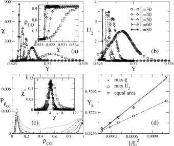
Figure 1: The ZGB model. (a) The order parameter $\rho_{CO}$ (inset) and its variance $\chi$ versus the creation probability $Y$. (b) The moment ratio $U_{2}$ versus $Y$. (c) The (non-normalized) order parameter QS probability distribution at the equal area condition. Inset: data collapse analysis from the relations ${\chi}^{*}=\chi/L^{2}$ and $y^{*}=(Y-Y_{0})L^{2}$. (d) Scaling of $Y_{L}$ as function of $1/L^{2}$.

Consider the Ziff-Gulari-Barshad (ZGB) model zgb , which reproduces relevant features of carbon monoxide oxidation on a catalytic surface (a lattice whose sites can be either empty or occupied by an oxygen atom O or a carbon monoxide molecule CO). CO (O₂) reach the surface with probability $Y$ ($1-Y$). Whenever a CO encounters a vacant site, the site becomes occupied. If a O₂ molecule encounters two nearest-neighbor empty sites, it dissociates filling the two sites. If 2 atoms O and 1 atom C reach an elementary $2\times 2$ lattice cell, they immediately form CO₂ and desorb. The model exhibits two transitions – regulated by the $CO$ molecules fraction, $\rho_{CO}$ – each between an active steady and an absorbing (poisoned) state. For large (extreme low) $Y$, the surface becomes saturated by CO (O). The former (latter) transition is discontinuous (continuous, belonging to the DP universality). The discontinuous transition is shown in Fig. 1. The $Y$ region of rapid increase of $\rho_{CO}$ (inset of (a)) corresponds to the maxima of $\chi$ and $U_{2}$ (which increase with $L^{2}$, Fig. 1 (a) and (b)) and their location scale with $1/L^{2}$, Fig. 1 (d). So we estimate $Y_{0}=0.5253(3)$ (max. of $\chi$) and $Y_{0}=0.5254(3)$ (max. of $U_{2}$). The $Y_{L}$ for which the two peaks of $P_{\rho_{CO}}$, Fig. 1 (c), have the same area also scales with $1/L^{2}$. From this we estimate $Y_{0}=0.5253(3)$. These values are in excellent agreement among them and with $Y_{0}=0.5250(6)$, recently obtained by other means sinha . Defining ${\chi}^{*}=\chi/L^{2}$ and $y^{*}=(Y-Y_{0})L^{2}$, the collapsed data is shown in Fig. 1 (c) inset, confirming a $L^{2}$ scaling.

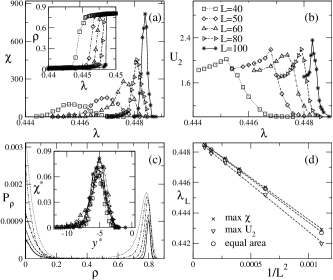
Figure 2: The 2SCP model. (a) The order parameter $\rho$ (inset) and its variance $\chi$ versus the creation rate $\lambda$. (b) The moment ratio $U_{2}$ versus $\lambda$. (c) The (non-normalized) order parameter QS probability distribution at the equal area condition. Inset: data collapse analysis from the relations ${\chi}^{*}=\chi/L^{2}$ and $y^{*}=(\lambda-\lambda_{0})L^{2}$. (d) Scaling of $\lambda_{L}$ as function of $1/L^{2}$.

For a two-species symbiotic contact process (2SCP) scp , any site is either empty or occupied by an element A, by an element B, or by one of each. Each individual reproduces (autocatalytic), creating a new at one of its first-neighbors sites at rate $\lambda_{A}=\lambda_{B}=\lambda$. In a single occupied site, A or B dies at unitary rate. Sole individuals follows the usual CP dynamics scp . However, in doubly occupied sites, due to symbiosis both A and B die at a reduced $\mu=$ const $<1$ rate. Besides the CP usual active (A and B populations fixed) and absorbing phases, there are two extra symmetric active phases, in which just one species exists.

If A and B diffuse with rate $D$, for $\mu\to 0$ the transition changes from continuous to discontinuous. The order parameter is the density of occupied sites $\rho$. Figure 2 exemplifies this 2SCP for $\mu=0.01$ and $D=0.1$, with a discontinuous transition between absorbing and active symmetric phases for $\lambda\approx 0.449$ scp . Like ZGB, in the transition region there are peaks for $\chi$ and $U_{2}$, Fig. 2 (a) and (b), whose maxima positions $\lambda_{L}$ increase with $1/L^{2}$, Fig. 2 (d). A $L\rightarrow\infty$ extrapolation yields $\lambda_{0}=0.4489(1)$ and $0.4490(1)$, respectively. The equal areas condition for $P_{\rho}$, Fig. 2 (c), shows a $1/L^{2}$ scaling, leading to $\lambda_{0}=0.4488(1)$. The estimates display excellent agreement among them and with Ref. scp . Finally, a fair data collapse is shown in Fig. 2 (c) inset.

We discuss a model of competitive interactions in bipartite ($k=$ A and B) sublattices martins , assuming the version in salete , so instead of critical martins , the phase diagram has three coexistence lines. Also, besides an absorbing, we have a spontaneous breaking symmetry transition. Given a site in the sublattice $k$, the number of particles in its first ($j=1$) and second ($j=2$) nearby neighborhood is $n_{jk}$. For $n^{(a)}_{jk}$ the number of adjacent particles in $j$, the dynamics is as the following salete . With probability $(1+\mu\,(n_{1k})^{2})/(\lambda_{1}+\lambda_{2}+1+\mu\,(n_{1k})^{2})$ we attempt to annihilate a randomly selected particle P. If P survives, we choose at will $j=1,2$. Then, with probability $p_{j}$ we try to create a new particle in a free site in the $j$ neighborhood of P, with $p_{j}=\lambda_{j}/(\lambda_{1}+\lambda_{2}+1+\mu\,(n_{1k})^{2})$ for $n^{(a)}_{jk}\geq j$ and zero otherwise (in martins , $\mu=\lambda_{2}=0$).

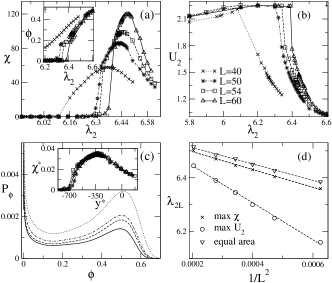
Figure 3: The competitive CP ab–as transition. (a) The order parameter $\phi$ (inset) and its variance $\chi$ versus the creation rate $\lambda_{2}$. (a) The order parameter variance $\chi$ versus the creation rate $\lambda_{2}$. (b) The moment ratio $U_{2}$ versus $\lambda_{2}$. (c) The (non-normalized) order parameter QS probability distribution at the equal area condition. Inset: data collapse analysis from the relations ${\chi}^{*}=\chi/L^{2}$ and $y^{*}=(\lambda_{2}-{\lambda_{2}}_{0})L^{2}$. (d) Scaling of ${\lambda_{2}}_{L}$ as function of $1/L^{2}$.

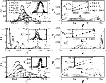
Figure 4: The second Schlögl model: versions SL1 in (a) and (b), SL2 in (c) and (d), and SL1 with time disorder in (e) and (f). Left panels, the order parameters variance $\chi$ versus $\alpha$ (insets: their collapsed plots). Right panels, the (non-normalized) order parameters QS probability distributions (insets: $\alpha_{L}$ as function of $1/L^{2}$).

The absorbing (ab)–active symmetric (as) phases line is discontinuous for lower $\lambda_{1}$. Proper order parameters are $\rho=(\rho_{A}+\rho_{B})/2$ and $\phi=|\rho_{A}-\rho_{B}|$, with $\rho_{X}$ the $X$-sublattice density. In the ab phase we have $\rho=\phi=0$, whereas for the as phase $\rho\neq 0$ and $\phi=0$. So, for the as phase, the sublattices are equally populated. From Fig. 3 we see that the ab–as transition follows our FSS.

Finally, we address two versions of the second Schlögl model schlogol72 : SL1 jensen ; paula , corresponding to a lattice version of the stochastic differential equation considered in martin2015 , and SL2 fiore14 , a modification of a pair contact process pcp . In SL$n$, a particle ($n=1$) [a pair of two adjacent particles ($n=2$)] is randomly selected and can be annihilated with probability $p_{0}=\alpha/(1+\alpha)$. If it is not, then:
(1) For SL1, a nearest neighbor site $i$ is chosen. If $i$ is empty, the particle diffuses to it. Otherwise, with probability $p=0.5$ jensen ; paula a new particle is created and placed at will in a neighboring empty site;
(2) If for SL2 there is at least $nn_{p}>1$ other pairs in the original pair neighborhood, a new particle can be created with rate $nn_{p}/4$ in an available site in this same neighborhood.

SL1 (SL2) presents single (infinite) AS, with the order parameter being the particle density $\rho$ (pair density $\phi$). The transitions occur close to $\alpha=0.0747$ (SL1) paula and $\alpha=0.0480$ (SL2) fiore14 . Results are summarized in Fig. 4. For both models our $\alpha_{L}$’s scale with $1/L^{2}$. For SL1, we obtain $\alpha_{0}=0.0742(1)$ (maximum of $\chi$), $0.0743(1)$ (maximum of $U_{2}$) and $0.0742(1)$ (equal areas). All estimates agree very well and are close to $0.0747$ in paula (calculated from the threshold separating ongoing active state and an exponential decay of $\rho$, considering a fully occupied initial configuration). For SL2 $\alpha_{0}=0.0473(1)$ (maximum of $\chi$), $0.0472(1)$ (maximum of $U_{2}$) and $0.0472(1)$ (equal areas), all close to $0.0480$ in fiore14 (derived from the onset for the decay of $\phi$ towards the absorbing regime).

Lastly, we incorporate temporal disorder into the SL1 model by assuming that at each instance, the creation probability, $1-p_{0}$, is $\mbox{Min}\{1/(1+\alpha)+\delta,1\}$, with $\delta$ randomly chosen within $[-\sigma,\sigma]$. Results for $\sigma=0.15$ are shown in Fig. 4 (e) and (f). Here also $\alpha_{L}$’s scales with $1/L^{2}$, from which we obtain $\alpha_{0}=0.0680(1)$ (maximum of $\chi$), $0.0683(2)$ (maximum of $U_{2}$) and $0.0680(1)$ (equal areas). Similar conclusions are obtained for $\sigma=0.25$ (not shown), from which $\alpha_{0}=0.0265(1)$ (maximum of $\chi$ and equal areas). So, in contrast to spatial disorder martin2015 , the present is the first evidence that temporal disorder does not hinder discontinuous absorbing phase transitions (but obviously, more studies should be in order, see, e.g., vazquez-2010 ).

In summary, we propose a general FSS theory for discontinuous NeqPTs to AS. From QS ideas, we obtain an effective system – which reproduces the thermodynamic properties of the original problem – undergoing ‘normal’ (i.e., not to AS) discontinuous phase transitions. Moreover it is described by a bimodal distribution for the order parameter, so allowing inference of the $V$ scaling behavior. The only eventual difficulty to implement such universal scheme would be if the particular system hinders a QSPD. However, the known examples displaying such feature are very specific problem . Our study is particularly useful given that this class of NeqPTs have no equilibrium counterparts and there are no universal treatments for discontinuous absorbing phase transitions for $d\geq 2$.

We acknowledge CNPq, Capes, CT-Infra and Fapesp for research grants. We are in debt to Hans J. Herrmann and Mario de Oliveira for insightful discussions.

References

- (1) J. Marro and R. Dickman, Nonequilibrium Phase Transitions in Lattice Models (Cambridge University Press, Cambridge, 1999).
- (2) G. Ódor, Universality in Nonequilibrium Lattice Systems: Theoretical Foundations (World Scientific, Singapore, 2007)
- (3) M. Henkel, H. Hinrichsen, and S. Lubeck, Non-Equilibrium Phase Transitions Volume I: Absorbing Phase Transitions (Springer-Verlag, Dordrecht, 2008).
- (4) H. Hinrichsen, Adv. Phys. 49, 815 (2000).
- (5) G. Ódor, Rev. Mod. Phys. 76, 663 (2004).
- (6) K. A. Takeuchi, M. Kuroda, H. Chaté, and M. Sano, Phys. Rev. Lett. 99, 234503 (2007).
- (7) L. Corté, P. M. Chaikin, J. P. Gollub, and D. J. Pine, Nature Physics 4, 420 (2008).
- (8) S. Okuma, Y. Tsugawa, and A. Motohashi, Phys. Rev. B 83, 012503 (2011).
- (9) S. Lubeck, Int. J. Mod. Phys. B 18, 3977 (2004).
- (10) M. Henkel and M. Pleimling, Non-Equilibrium Phase Transitions Volume II: Ageing and Dynamical Scale (Springer-Verlag, Dordrecht, 2010).
- (11) C. E. Fiore, Phys. Rev. E 89, 022104 (2014).
- (12) E. F. da Silva and M. J. de Oliveira, J. Phys. A 44, 135002 (2011); ibid, Comp. Phys. Comm. 183, 2001 (2012).
- (13) P. V. Martín, J. A. Bonachela, S. A. Levin, and M. A. Muñoz, PNAS 112, E1828 (2015).
- (14) R. M. Ziff, E. Gulari, and Y. Barshad, Phys. Rev. Lett. 56, 2553 (1986).
- (15) M. Ehsasi, M. Matloch, O. Frank, J. H. Block, K. Christmann, F. S. Rys, and W. Hirschwald, J. Chem. Phys. 91, 4949 (1989).
- (16) M. M. de Oliveira, R. V. Santos, and R. Dickman, Phys. Rev. E 86, 011121 (2012); M. M. de Oliveira and R. Dickman, Phys. Rev. E 90, 032120 (2014).
- (17) H. Weissmann and N. M. Shnerb, EPL 106, 28004 (2014).
- (18) B. Néel, I. Rondini, A. Turzillo, N. Mujica, and R. Soto, Phys. Rev. E 89, 042206 (2014).
- (19) G. O. Cardozo and J. F. Fontanari, Physica A 359, 478 (2006).
- (20) L. Chen, F. Ghanbarnejad, W. Cai, and P. Grassberger, EPL 104, 50001 (2013).
- (21) N. Crokidakis and E. Brigatti. J. Stat. Mech. P01019 (2015).
- (22) C. Castellano, M. Marsili, and A. Vespignani, Phys. Rev. Lett. 85, 3536 (2000).
- (23) S. Lübeck, J. Stat. Phys. 123, 193 (2006).
- (24) P. Grassberger, J. Stat. Mech. P01004 (2006).
- (25) H. Hinrichsen, eprint: cond-mat/0006212 (2000).
- (26) M. E. Fisher and A. N. Berker, Phys. Rev. B 26, 2507 (1982).
- (27) K. Binder and D. P. Landau, Phys. Rev. B 30, 1477 (1984).
- (28) M. S. S. Challa, D. P. Landau, and K. Binder, Phys. Rev. B 34, 1841 (1986).
- (29) K. Binder, Rep. Prog. Phys. 50, 783 (1987).
- (30) J. Lee and J. M. Kosterlitz, Phys. Rev. B 43, 3265 (1991).
- (31) C. Borgs and R. Kotecký, J. Stat. Phys. 61, 79 (1990); ibid, Phys. Rev. Lett. 68, 1734 (1992).
- (32) D. P. Landau and K. Binder, A guide to Monte Carlo Simulations in Statistical Physics, (Cambridge University Press, Cambridge, 2000).
- (33) C. E. Fiore and M. G. E. da Luz, Phys. Rev. Lett. 107, 230601 (2011).
- (34) E. Machado, G. M. Buendía, and P. A. Rikvold, Phys. Rev. E 71, 031603 (2005).
- (35) M. A. Saif and P. M. Gade, J. Stat. Mech. P07023 (2009).
- (36) I. Sinha and A. K. Mukherjee, J. Stat. Phys. 146, 669 (2012).
- (37) H. Hinrichsen, Physica A 369, 1 (2006); R. A. Blythe, J. Phys.: Conf. Ser. 40, 1 (2006); R. Brak, J. de Gier, V. Rittenberg; J. Phys. A 37, 4303 (2004); R. A. Blythe, M. R. Evans; Phys. Rev. Lett. 87, 080601 (2002).
- (38) M. M. de Oliveira and R. Dickman, Phys. Rev. E 71, 016129 (2005); ibid Braz. J. Phys. 36, 685 (2006).
- (39) R. Dickman and R. Vidigal, J. Phys. A 35, 1147 (2002).
- (40) I. Nȧsell, J. Theor. Biol. 211, 11 (2001).
- (41) For micro-configurations, their transition rate, and the probabiliy of , the global balance implies .
- (42) F. Schlögol, Z. Phys. 253, 147 (1972).
- (43) M. M. de Oliveira and R. Dickman, Physica A 343, 525 (2004).
- (44) K. Mallick, Pramana 73, 417 (2009); T. Tomé and M. J. de Oliveira Phys. Rev. Lett. 108, 020601 (2012).
- (45) J. Keizer, Statistical Thermodynamics of Nonequilibrium Processes (Springer-Verlag, New York, 1987); H. Larralde and D. P. Sanders, J. Phys. A 42, 335002 (2009).
- (46) Claudio Landim, Aniura Milanés, Stefano Olla, Markov Proc. Rel. Fields 14, 165 (2008); M. Cramer, C. M. Dawson, J. Eisert, T. J. Osborne Phys. Rev. Lett. 100, 030602 (2008); M Cramer and J Eisert, New J. Phys. 12, 055020 (2010).
- (47) Terms are unimportant around the transition point for large ’s.
- (48) M. M. de Oliveira and R. Dickman, Phys. Rev. E 84, 011125 (2011).
- (49) S. Pianegonda and C. E. Fiore, J. Stat. Mech. P05008, (2014).
- (50) A. Windus and H. J. Jensen, J. Phys. A 40, 2287 (2007).
- (51) P. V. Martín, J. A. Bonachela, and M. A. Muñoz, Phys. Rev. E 89, 012145 (2014).
- (52) J. K. L. da Silva and R. Dickman, Phys. Rev. E 60, 5126 (1999).
- (53) F. Vazquez, C. López, J. M. Calabrese, M. A. Muñoz, J. Theor. Biol. 264, 360 (2010).
- (54) A. D. Barbour and P. K. Pollett, J. Appl. Probab. 47, 934 (2010); A. D. Barbour and P. K. Pollett, Stoc. Process. Applic. 122, 3740 (2012); P. Groisman and M. Jonckheere, Markov Process. Relat. Fields 19, 521 (2013).