On the convergence analysis of the optimized gradient method

Abstract

This paper considers the problem of unconstrained minimization of smooth convex functions having Lipschitz continuous gradients with known Lipschitz constant. We recently proposed an optimized gradient method (OGM) kim::ofo for this problem and showed that it has a worst-case convergence bound for the cost function decrease that is twice as small as that of Nesterov’s fast gradient method (FGM) nesterov:83:amf , yet has a similarly efficient practical implementation. Drori drori:16:tei showed recently that OGM has optimal complexity over the general class of first-order methods. This optimality makes it important to study fully the convergence properties of OGM. The previous worst-case convergence bound for OGM was derived for only the last iterate of a secondary sequence. This paper provides an analytic convergence bound for the primary sequence generated by OGM. We then discuss additional convergence properties of OGM, including the interesting fact that OGM has two types of worst-case functions: a piecewise affine-quadratic function and a quadratic function. These results help complete the theory of optimal first-order methods for smooth convex minimization.

1 Introduction

Consider the unconstrained smooth convex minimization problem

$$\min_{\bm{x}\in\mathbb{R}^{d}}\; \;f(\bm{x})$$ (M)

with the following three conditions:

• $f\;:\;\mathbb{R}^{d}\rightarrow\mathbb{R}$ is a convex function of the type $\mathcal{C}_{L}^{1,1}(\mathbb{R}^{d})$, i.e., continuously differentiable with Lipschitz continuous gradient:

  $$||\nabla f(\bm{x})-\nabla f(\bm{y})||\leq L||\bm{x}-\bm{y}||,\quad\forall\bm{x},\bm{y}\in\mathbb{R}^{d},$$

  where $L>0$ is the Lipschitz constant.

• The optimal set $X_{*}(f)=\mathop{\operator@font arg\,min}_{\bm{x}\in\mathbb{R}^{d}}f(\bm{x})$ is nonempty, i.e., problem (M) is solvable.

• The distance between the initial point $\bm{x}_{0}$ and an optimal solution $\bm{x}_{*}\in X_{*}(f)$ is bounded by $R>0$, i.e., $||\bm{x}_{0}-\bm{x}_{*}||\leq R$.

We use $\mathcal{F}_{L}(\mathbb{R}^{d})$ to denote the class of functions that satisfy the above conditions hereafter.

For large-scale optimization problems of type (M) that arise in various fields such as communications, machine learning and signal processing, general first-order algorithms that query only the cost function values and gradients are attractive because of their mild dependence on the problem dimension cevher:14:cof . For simplicity, we initially focus on the class of fixed-step first-order (FO) algorithms having the following form:

Algorithm Class FO $\displaystyle\text{Input: }f\in\mathcal{F}_{L}(\mathbb{R}^{d}),\;\bm{x}_{0}\in\mathbb{R}^{d}.$ $\displaystyle\text{For }i=0,\ldots,N-1$ $\displaystyle\quad\bm{x}_{i+1}=\bm{x}_{i}-\frac{1}{L}\sum_{k=0}^{i}h_{i+1,k}\nabla f(\bm{x}_{k})$ (1.1)

FO updates use weighted sums of current and previous gradients $\{\nabla f(\bm{x}_{k})\}_{k=0}^{i}$ with (pre-determined) step sizes $\{h_{i+1,k}\}_{k=0}^{i}$ and the Lipschitz constant $L$. Class FO includes the (fixed-step) gradient method (GM), the heavy-ball method polyak:64:smo , Nesterov’s fast gradient method (FGM) nesterov:83:amf ; nesterov:05:smo , and the recently introduced optimized gradient method (OGM) kim::ofo . Those four methods have efficient recursive formulations rather than directly using (1.1) that would require storing all previous gradients and computing weighted summations every iteration. Among class FO, Nesterov’s FGM has been used widely, since it achieves the optimal rate $O({1}/{N^{2}})$ for decreasing a cost function in $N$ iterations nesterov:04 , and has two efficient forms as shown below for smooth convex problems.

Algorithm FGM1 nesterov:83:amf $\displaystyle\text{Input: }f\in\mathcal{F}_{L}(\mathbb{R}^{d}),\;\bm{x}_{0}\in\mathbb{R}^{d},\;\bm{y}_{0}=\bm{x}_{0},\;t_{0}=1.$ $\displaystyle\text{For }i=0,\ldots,N-1$ $\displaystyle\quad\bm{y}_{i+1}=\bm{x}_{i}-\frac{1}{L}\nabla f(\bm{x}_{i})$ $\displaystyle\quad t_{i+1}=\frac{1+\sqrt{1+4t_{i}^{2}}}{2},$ $\displaystyle\quad\bm{x}_{i+1}=\bm{y}_{i+1}+\frac{t_{i}-1}{t_{i+1}}(\bm{y}_{i+1}-\bm{y}_{i})$     Algorithm FGM2 nesterov:05:smo $\displaystyle\text{Input: }f\in\mathcal{F}_{L}(\mathbb{R}^{d}),\;\bm{x}_{0}\in\mathbb{R}^{d},\;\bm{y}_{0}=\bm{x}_{0},\;t_{0}=1.$ $\displaystyle\text{For }i=0,\ldots,N-1$ $\displaystyle\quad\bm{y}_{i+1}=\bm{x}_{i}-\frac{1}{L}\nabla f(\bm{x}_{i})$ $\displaystyle\quad\bm{z}_{i+1}=\bm{x}_{0}-\frac{1}{L}\sum_{k=0}^{i}t_{k}\nabla f(\bm{x}_{k})$ $\displaystyle\quad t_{i+1}=\frac{1+\sqrt{1+4t_{i}^{2}}}{2},$ $\displaystyle\quad\bm{x}_{i+1}=\left(1-\frac{1}{t_{i+1}}\right)\bm{y}_{i+1}+\frac{1}{t_{i+1}}\bm{z}_{i+1}$

Both FGM1 and FGM2 produce identical sequences $\{\bm{y}_{i}\}$ and $\{\bm{x}_{i}\}$, where the primary sequence $\{\bm{y}_{i}\}$ satisfies the following convergence bound nesterov:83:amf ; nesterov:05:smo for any $1\leq i\leq N$:

$$f(\bm{y}_{i})-f(\bm{x}_{*})\leq\frac{LR^{2}}{2t_{i-1}^{2}}\leq\frac{2LR^{2}}{(i+1)^{2}}.$$ (1.2)

In kim::ofo , we showed that the secondary sequence $\{\bm{x}_{i}\}$ of FGM satisfies the following convergence bound that is similar to (1.2) for any $1\leq i\leq N$:

$$f(\bm{x}_{i})-f(\bm{x}_{*})\leq\frac{LR^{2}}{2t_{i}^{2}}\leq\frac{2LR^{2}}{(i+2)^{2}}.$$ (1.3)

Taylor et al. taylor::ssc demonstrated that the upper bounds (1.2) and (1.3) are only asymptotically tight.

When the large-scale condition “$d\geq 2N+1$” holds, Nesterov nesterov:04 showed that for any first-order method generating $\bm{x}_{N}$ after $N$ iterations there exists a function $\phi$ in $\mathcal{F}_{L}(\mathbb{R}^{d})$ that satisfies the following lower bound:

$$\frac{3L||\bm{x}_{0}-\bm{x}_{*}||^{2}}{32(N+1)^{2}}\leq\phi(\bm{x}_{N})-\phi(\bm{x}_{*}).$$ (1.4)

Although FGM achieves the optimal rate $O({1}/{N^{2}})$, one can still seek algorithms that improve upon the constant factor in (1.2) and (1.3), in light of the gap between the bounds (1.2), (1.3) of FGM and the lower complexity bound (1.4). Building upon Drori and Teboulle (hereafter “DT”)’s approach drori:14:pof of seeking FO methods that are faster than Nesterov’s FGM (reviewed in Section 2.3), we recently proposed following two efficient formulations of OGM kim::ofo .

Algorithm OGM1 $\displaystyle\text{Input: }f\in\mathcal{F}_{L}(\mathbb{R}^{d}),\;\bm{x}_{0}\in\mathbb{R}^{d},\;\bm{y}_{0}=\bm{x}_{0},\;\theta_{0}=1.$ $\displaystyle\text{For }i=0,\ldots,N-1$ $\displaystyle\quad\bm{y}_{i+1}=\bm{x}_{i}-\frac{1}{L}\nabla f(\bm{x}_{i})$ $\displaystyle\quad\theta_{i+1}=\begin{cases}\frac{1+\sqrt{1+4\theta_{i}^{2}}}{2},&i\leq N-2\\ \frac{1+\sqrt{1+8\theta_{i}^{2}}}{2},&i=N-1\end{cases}$ $\displaystyle\quad\bm{x}_{i+1}=\bm{y}_{i+1}+\frac{\theta_{i}-1}{\theta_{i+1}}(\bm{y}_{i+1}-\bm{y}_{i})$ $\displaystyle\hskip 120.0pt+\frac{\theta_{i}}{\theta_{i+1}}(\bm{y}_{i+1}-\bm{x}_{i})$     Algorithm OGM2 $\displaystyle\text{Input: }f\in\mathcal{F}_{L}(\mathbb{R}^{d}),\;\bm{x}_{0}\in\mathbb{R}^{d},\;\bm{y}_{0}=\bm{x}_{0},\;\theta_{0}=1.$ $\displaystyle\text{For }i=0,\ldots,N-1$ $\displaystyle\quad\bm{y}_{i+1}=\bm{x}_{i}-\frac{1}{L}\nabla f(\bm{x}_{i})$ $\displaystyle\quad\bm{z}_{i+1}=\bm{x}_{0}-\frac{1}{L}\sum_{k=0}^{i}2\theta_{k}\nabla f(\bm{x}_{k})$ $\displaystyle\quad\theta_{i+1}=\begin{cases}\frac{1+\sqrt{1+4\theta_{i}^{2}}}{2},&i\leq N-2\\ \frac{1+\sqrt{1+8\theta_{i}^{2}}}{2},&i=N-1\end{cases}$ $\displaystyle\quad\bm{x}_{i+1}=\left(1-\frac{1}{\theta_{i+1}}\right)\bm{y}_{i+1}+\frac{1}{\theta_{i+1}}\bm{z}_{i+1}$

OGM1 and OGM2 have computational efficiency comparable to FGM1 and FGM2, and produce identical primary sequence $\{\bm{y}_{i}\}$ and secondary sequence $\{\bm{x}_{i}\}$. The last iterate $\bm{x}_{N}$ of OGM satisfies the following analytical worst-case bound (kim::ofo, , Theorem 2):

$$f(\bm{x}_{N})-f(\bm{x}_{*})\leq\frac{LR^{2}}{2\theta_{N}^{2}}\leq\frac{LR^{2}}{(N+1)(N+1+\sqrt{2})},$$ (1.5)

which is twice as small as those for FGM in (1.2) and (1.3). Recently for the condition “$d\geq N+1$”, Drori drori:16:tei showed that for any first-order method there exists a function $\psi$ in $\mathcal{F}_{L}(\mathbb{R}^{d})$ that cannot be minimized faster than the following lower bound:

$$\frac{L||\bm{x}_{0}-\bm{x}_{*}||^{2}}{2\theta_{N}^{2}}\leq\psi(\bm{x}_{N})-\psi(\bm{x}_{*}),$$ (1.6)

where $\bm{x}_{N}$ is the $N$th iterate of any first-order method. This lower complexity bound (1.6) improves on (1.4), and exactly matches the bound (1.5) of OGM, showing that OGM achieves the optimal worst-case bound of the cost function for first-order methods when $d\geq N+1$. What is remarkable about Drori’s result is that OGM was derived by optimizing over the class FO having fixed step sizes, leading to (1.5), whereas Drori’s lower bound in (1.6) is for the general class of first-order methods where the step sizes are arbitrary. It is interesting that OGM with its fixed step sizes is optimal over the apparently much broader class.

Because OGM has such optimality, it is desirable to understand its properties thoroughly. For example, analytical bounds for the primary sequence $\{\bm{y}_{i}\}$ of OGM have not been studied previously, although numerical bounds were discussed by Taylor et al. taylor::ssc . This paper provides analytical bounds for the primary sequence of OGM, augmenting the convergence analysis of $\bm{x}_{N}$ of OGM given in kim::ofo . We also relate OGM to another version of Nesterov’s accelerated first-order method in nesterov:13:gmf that has a similar formulation as OGM2.

In (kim::ofo, , Theorem 3), we specified a worst-case function for which OGM achieves the first upper bound in (1.5) exactly. The corresponding worst-case function is the following piecewise affine-quadratic function:

$$f_{\mathrm{1,OGM}}(\bm{x};N)=\begin{cases}\frac{LR}{\theta_{N}^{2}}||\bm{x}||-\frac{LR^{2}}{2\theta_{N}^{4}},&\text{if }||\bm{x}||\geq\frac{R}{\theta_{N}^{2}},\\ \frac{L}{2}||\bm{x}||^{2},&\text{otherwise,}\end{cases}$$ (1.7)

where OGM iterates remain in the affine region with the same gradient value (without overshooting) for all $N$ iterations. Section 4 shows that a simple quadratic function is also a worst-case function for OGM, and describes why it is interesting that the optimal OGM has these two types of worst-case functions.

Section 2 reviews DT’s Performance Estimation Problem (PEP) framework in drori:14:pof that enables systematic worst-case performance analysis of optimization methods. Section 3 provides new convergence analysis for the primary sequence of OGM. Section 4 discusses the two types of worst-case functions for OGM, and Section 5 concludes.

2 Prior work: Performance Estimation Problem (PEP)

Exploring the convergence performance of optimization methods including class FO has a long history. DT drori:14:pof were the first to cast the analysis of the worst-case performance of optimization methods into an optimization problem called PEP, reviewed in this section. We also review how we developed OGM kim::ofo that is built upon DT’s PEP.

2.1 Review of PEP

To analyze the worst-case convergence behavior of a method in class FO having given step sizes $\bm{h}=\{h_{i,k}\}_{0\leq k<i\leq N}$, DT’s PEP drori:14:pof bounds the decrease of the cost function after $N$ iterations as

$$\mathcal{B}_{\mathrm{P}}(\bm{h},N,d,L,R)\triangleq\; \max_{\begin{subarray}{c}f\in\mathcal{F}_{L}(\mathbb{R}^{d}),\\ \bm{x}_{0},\cdots,\bm{x}_{N}\in\mathbb{R}^{d},\\ \bm{x}_{*}\in X_{*}(f)\end{subarray}}f(\bm{x}_{N})-f(\bm{x}_{*})$$ (P)

$$\text{s.t.}\>\;||\bm{x}_{0}-\bm{x}_{*}||\leq R,\quad\bm{x}_{i+1}=\bm{x}_{i}-\frac{1}{L}\sum_{k=0}^{i}h_{i+1,k}\nabla f(\bm{x}_{k}),\quad i=0,\ldots,N-1,$$

for given dimension $d$, Lipschitz constant $L$ and the distance $R$ between an initial point $\bm{x}_{0}$ and an optimal point $\bm{x}_{*}\in X_{*}(f)$.

Since problem (P) is difficult to solve, DT drori:14:pof introduced a series of relaxations. Then the upper bound of the worst-case performance was found numerically in drori:14:pof by solving a relaxed PEP problem. For some cases, analytical worst-case bounds were revealed in drori:14:pof ; kim::ofo , where some of those analytical bounds were even found to be exact despite the relaxations. On the other hand, Taylor et al. taylor::ssc studied the numerical tight worst-case bound of (P) by avoiding DT’s one relaxation step that is not guaranteed to be tight and showing the tightness of the rest of DT’s relaxations in drori:14:pof (for the condition “$d\geq N+2$”).

To summarize recent PEP studies, DT extended the PEP approach for nonsmooth convex problems drori::aov , Drori’s thesis drori:14:phd includes an extension of PEP to projected gradient methods for constrained smooth convex problems, and Taylor et al. taylor:15:ewc studied PEP for various first-order algorithms for solving composite convex problems. Similarly but using different relaxations of (P), Lessard et al. lessard:16:aad applied the Integral quadratic constraints to (P), leading to simpler computation but slightly looser convergence upper bounds.

The next two sections review relaxations of DT’s PEP and an approach for optimizing the choice of $\bm{h}$ for FO using PEP in drori:14:pof .

2.2 Review of DT’s relaxation on PEP

This section reviews relaxations introduced by DT to make (P) into a simpler semidefinite programming (SDP) problem. DT first relax the functional constraint $f\in\mathcal{F}_{L}(\mathbb{R}^{d})$ by a well-known property of the class of $\mathcal{F}_{L}(\mathbb{R}^{d})$ functions in (nesterov:04, , Theorem 2.1.5) and then further relax as follows:

$$\mathcal{B}_{\mathrm{P1}}(\bm{h},N,d,L,R)\triangleq\; \max_{\begin{subarray}{c}\bm{G}\in\mathbb{R}^{(N+1)d},\\ \bm{\delta}\in\mathbb{R}^{N+1}\end{subarray}}LR^{2}\delta_{N}$$ (P1)

$$\text{s.t.}\>\;\frac{1}{2}||\bm{g}_{i-1}-\bm{g}_{i}||^{2}\leq\delta_{i-1}-\delta_{i}-\left\langle\bm{g}_{i},\ \sum_{k=0}^{i-1}h_{i,k}\bm{g}_{k}\right\rangle,\quad i=1,\ldots,N,$$

$$\qquad\!\frac{1}{2}||\bm{g}_{i}||^{2}\leq-\delta_{i}-\left\langle\bm{g}_{i},\ \sum_{j=1}^{i}\sum_{k=0}^{j-1}h_{j,k}\bm{g}_{k}+\bm{\nu}\right\rangle,\quad i=0,\ldots,N,$$

for any given unit vector $\bm{\nu}\in\mathbbm{R}^{d}$, where we denote $\bm{g}_{i}\triangleq\frac{1}{L||\bm{x}_{0}-\bm{x}_{*}||}\nabla f(\bm{x}_{i})$ and $\delta_{i}\triangleq\frac{1}{L||\bm{x}_{0}-\bm{x}_{*}||^{2}}(f(\bm{x}_{i})-f(\bm{x}_{*}))$ for $i=0,\ldots,N,*$, and define $\bm{G}=[\bm{g}_{0}\cdots\bm{g}_{N}]^{\top}\in\mathbb{R}^{(N+1)\times d}$ and $\bm{\delta}=[\delta_{0}\cdots\delta_{N}]^{\top}\in\mathbb{R}^{N+1}$.

Maximizing relaxed problem (P1) is still difficult, so DT drori:14:pof use a duality approach on (P1). Replacing $\max_{\bm{G},\bm{\delta}}LR^{2}\delta_{N}$ by $\min_{\bm{G},\bm{\delta}}-\delta_{N}$ for convenience, the Lagrangian of the corresponding constrained minimization problem (P1) with dual variables $\bm{\lambda}=(\lambda_{1},\cdots,\lambda_{N})^{\top}\in\mathbb{R}_{+}^{N}$ and $\bm{{\tau}}=(\tau_{0},\cdots,\tau_{N})^{\top}\in\mathbb{R}_{+}^{N+1}$ becomes

$$\mathcal{L}(\bm{G},\bm{\delta},\bm{\lambda},\bm{{\tau}};\bm{h})\triangleq-\delta_{N}+\sum_{i=1}^{N}\lambda_{i}(\delta_{i}-\delta_{i-1})+\sum_{i=0}^{N}\tau_{i}\delta_{i}+\mathop{{}\mathsf{Tr}\!\left\{\bm{G}^{\top}\bm{S}(\bm{h},\bm{\lambda},\bm{{\tau}})\bm{G}+\bm{\nu}\bm{{\tau}}^{\top}\bm{G}\right\}}\nolimits,$$ (2.1)

where

$$\begin{cases}\bm{S}(\bm{h},\bm{\lambda},\bm{{\tau}})\triangleq\sum_{i=1}^{N}\lambda_{i}\bm{A}_{i-1,i}(\bm{h})+\sum_{i=0}^{N}\tau_{i}\bm{D}_{i}(\bm{h}),&\\ \bm{A}_{i-1,i}(\bm{h})\triangleq\frac{1}{2}(\bm{u}_{i-1}-\bm{u}_{i})(\bm{u}_{i-1}-\bm{u}_{i})^{\top}+\frac{1}{2}\sum_{k=0}^{i-1}h_{i,k}(\bm{u}_{i}\bm{u}_{k}^{\top}+\bm{u}_{k}\bm{u}_{i}^{\top}),&\\ \bm{D}_{i}(\bm{h})\triangleq\frac{1}{2}\bm{u}_{i}\bm{u}_{i}^{\top}+\frac{1}{2}\sum_{j=1}^{i}\sum_{k=0}^{j-1}h_{j,k}(\bm{u}_{i}\bm{u}_{k}^{\top}+\bm{u}_{k}\bm{u}_{i}^{\top}),&\end{cases}$$ (2.2)

and $\bm{u}_{i}=\bm{e}_{i+1}\in\mathbbm{R}^{N+1}$ is the $(i+1)$th standard basis vector.

Using further derivations of a duality approach on (2.1) in drori:14:pof , the dual problem of (P1) becomes the following SDP problem:

$$\mathcal{B}_{\mathrm{P}}(\bm{h},N,d,L,R)\leq \mathcal{B}_{\mathrm{D}}(\bm{h},N,L,R)\triangleq\min_{\begin{subarray}{c}(\bm{\lambda},\bm{{\tau}})\in\Lambda,\\ \gamma\in\mathbb{R}\end{subarray}}\left\{\frac{1}{2}LR^{2}\gamma\;:\;\left(\begin{array}[]{cc}\bm{S}(\bm{h},\bm{\lambda},\bm{{\tau}})&\frac{1}{2}\bm{{\tau}}\\ \frac{1}{2}\bm{{\tau}}^{\top}&\frac{1}{2}\gamma\end{array}\right)\succeq 0\right\},$$ (D)

where

$$\Lambda=\left\{(\bm{\lambda},\bm{{\tau}})\in\mathbbm{R}_{+}^{N}\times\mathbbm{R}_{+}^{N+1}\;:\;\begin{array}[]{l}\tau_{0}=\lambda_{1},\quad\lambda_{N}+\tau_{N}=1,\\ \lambda_{i}-\lambda_{i+1}+\tau_{i}=0,\;i=1,\ldots,N-1,\end{array}\right\}.$$

Then, for given $\bm{h}$, the bound $\mathcal{B}_{\mathrm{D}}(\bm{h},N,L,R)$ (that is not guaranteed to be tight) can be numerically computed using any SDP solver, while analytical upper bounds $\mathcal{B}_{\mathrm{D}}(\bm{h},N,L,R)$ for some choices of $\bm{h}$ were found in drori:14:pof ; kim::ofo . Section 3 finds a new analytical upper bound for a modified version of $\mathcal{B}_{\mathrm{D}}$.

2.3 Review of optimizing the step sizes using PEP

In addition to finding upper bounds for given FO methods, DT drori:14:pof searched for the best FO methods with respect to the worst-case performance. Ideally one would like to optimize $\bm{h}$ over problem (P):

$$\bm{\hat{h}}_{\mathrm{P}}\triangleq\mathop{\operator@font arg\,min}_{\bm{h}\in\mathbb{R}^{{N(N+1)}/{2}}}\mathcal{B}_{\mathrm{P}}(\bm{h},N,d,L,R).$$ (HP)

However, optimizing (HP) directly seems impractical, so DT minimized the dual problem (D) using a SDP solver over the coefficients $\bm{h}$ as

$$\bm{\hat{h}}_{\mathrm{D}}\triangleq\mathop{\operator@font arg\,min}_{\bm{h}\in\mathbb{R}^{{N(N+1)}/{2}}}\mathcal{B}_{\mathrm{D}}(\bm{h},N,L,R).$$ (HD)

Due to relaxations, the computed $\bm{\hat{h}}_{\mathrm{D}}$ is not guaranteed to be optimal for problem (HP). Nevertheless, we show in kim::ofo that solving (HD) leads to an algorithm (OGM) having a convergence bound that is twice as small as that of FGM. Interestingly, OGM is optimal among first-order methods with $d\geq N+1$ drori:16:tei , i.e., $\bm{\hat{h}}_{\mathrm{D}}$ is a solution of both (HP) and (HD) for $d\geq N+1$. An optimal point $(\bm{\hat{h}},\bm{\hat{\lambda}},\bm{{\hat{\tau}}},\hat{\gamma})$ of (HD) is given in (kim::ofo, , Lemma 4 and Proposition 3) as follows:

$$\hat{h}_{i+1,k} =\begin{cases}\frac{\theta_{i}-1}{\theta_{i+1}}\hat{h}_{i,k},&k=0,\ldots,i-2,\\ \frac{\theta_{i}-1}{\theta_{i+1}}(\hat{h}_{i,i-1}-1),&k=i-1,\\ 1+\frac{2\theta_{i}-1}{\theta_{i+1}},&k=i,\end{cases}$$ (2.5)

$$=\begin{cases}\frac{1}{\theta_{i+1}}\left(2\theta_{k}-\sum_{j=k+1}^{i}\hat{h}_{j,k}\right),&k=0,\ldots,i-1,\\ 1+\frac{2\theta_{i}-1}{\theta_{i+1}},&k=i,\end{cases}$$ (2.6)

$$\hat{\lambda}_{i} =\frac{2\theta_{i-1}^{2}}{\theta_{N}^{2}},\quad i=1,\ldots,N,\quad\hat{\tau}_{i}=\begin{cases}\frac{2\theta_{i}}{\theta_{N}^{2}},&i=0,\ldots,N-1,\\ \frac{1}{\theta_{N}},&i=N,\end{cases}\quad\hat{\gamma}=\frac{1}{\theta_{N}^{2}}.$$ (2.7)

Thus both OGM1 and OGM2 satisfy the convergence bound (1.5) (kim::ofo, , Theorem 2, Propositions 4 and 5).

3 New convergence analysis for the primary sequence of OGM

3.1 Relaxed PEP for the primary sequence of OGM

This section applies PEP to an iterate $\bm{y}_{N}$ of the following class of fixed-step first-order methods (FO^′), complementing the worst-case performance of $\bm{x}_{N}$ in the previous section.

Algorithm Class FO^′ $\displaystyle\text{Input: }f\in\mathcal{F}_{L}(\mathbb{R}^{d}),\;\bm{x}_{0}\in\mathbb{R}^{d},\;\bm{y}_{0}=\bm{x}_{0}.$ $\displaystyle\text{For }i=0,\ldots,N$ $\displaystyle\quad\bm{y}_{i+1}=\bm{x}_{i}-\frac{1}{L}\nabla f(\bm{x}_{i})$ $\displaystyle\quad\bm{x}_{i+1}=\bm{x}_{i}-\frac{1}{L}\sum_{k=0}^{i}h_{i+1,k}\nabla f(\bm{x}_{k}).$

We first replace $f(\bm{x}_{N})-f(\bm{x}_{*})$ in (P) by $f(\bm{y}_{N+1})-f(\bm{x}_{*})$ as follows:

$$\mathcal{B}_{\mathrm{P^{\prime}}}(\bm{h},N,d,L,R)\triangleq\; \max_{\begin{subarray}{c}f\in\mathcal{F}_{L}(\mathbb{R}^{d}),\\ \bm{x}_{0},\cdots,\bm{x}_{N},\bm{y}_{N+1}\in\mathbb{R}^{d},\\ \bm{x}_{*}\in X_{*}(f)\end{subarray}}f(\bm{y}_{N+1})-f(\bm{x}_{*})$$ (P^′)

$$\text{s.t.}\>\;||\bm{x}_{0}-\bm{x}_{*}||\leq R,\quad\bm{y}_{N+1}=\bm{x}_{N}-\frac{1}{L}\nabla f(\bm{x}_{N}),$$

$$\qquad\!\bm{x}_{i+1}=\bm{x}_{i}-\frac{1}{L}\sum_{k=0}^{i}h_{i+1,k}\nabla f(\bm{x}_{k}),\quad i=0,\ldots,N-1.$$

We could directly repeat relaxations on (P^′) as reviewed in Section 2.2, but we found it difficult to solve a such relaxed problem of (P^′) analytically. Instead, we use the following inequality nesterov:04 :

$$f\left(\bm{x}-\frac{1}{L}\nabla f(\bm{x})\right)\leq f(\bm{x})-\frac{1}{2L}\left\|\nabla f(\bm{x})\right\|^{2},\quad\forall\bm{x}\in\mathbb{R}^{d}.$$ (3.1)

to relax (P^′), leading to the following bound:

$$\mathcal{B}_{\mathrm{P1}^{\prime}}(\bm{h},N,d,L,R)\triangleq\; \max_{\begin{subarray}{c}f\in\mathcal{F}_{L}(\mathbb{R}^{d}),\\ \bm{x}_{0},\cdots,\bm{x}_{N}\in\mathbb{R}^{d},\\ \bm{x}_{*}\in X_{*}(f)\end{subarray}}f(\bm{x}_{N})-\frac{1}{2L}||\nabla f(\bm{x}_{N})||^{2}-f(\bm{x}_{*})$$ (P1^′)

$$\text{s.t.}\>\;||\bm{x}_{0}-\bm{x}_{*}||\leq R,$$

$$\qquad\!\bm{x}_{i+1}=\bm{x}_{i}-\frac{1}{L}\sum_{k=0}^{i}h_{i+1,k}\nabla f(\bm{x}_{k}),\quad i=0,\ldots,N-1.$$

This bound has an additional term $-\frac{1}{2L}||\nabla f(\bm{x}_{N})||^{2}$ compared to (P). We later show that the increase of the worst-case upper bound due to this strict relaxation step using (3.1) is negligible asymptotically.

Similar to relaxing from (P) to (P1) in Section 2.2, we relax (P1^′) to the following bound:

$$\mathcal{B}_{\mathrm{P2}^{\prime}}(\bm{h},N,d,L,R)\triangleq\; \max_{\begin{subarray}{c}\bm{G}\in\mathbb{R}^{(N+1)d},\\ \bm{\delta}\in\mathbb{R}^{N+1}\end{subarray}}LR^{2}\left(\delta_{N}-\frac{1}{2}||\bm{g}_{N}||^{2}\right)$$ (P2^′)

$$\text{s.t.}\>\;\frac{1}{2}||\bm{g}_{i-1}-\bm{g}_{i}||^{2}\leq\delta_{i-1}-\delta_{i}-\left\langle\bm{g}_{i},\ \sum_{k=0}^{i-1}h_{i,k}\bm{g}_{k}\right\rangle,\quad i=1,\ldots,N,$$

$$\qquad\!\frac{1}{2}||\bm{g}_{i}||^{2}\leq-\delta_{i}-\left\langle\bm{g}_{i},\ \sum_{j=1}^{i}\sum_{k=0}^{j-1}h_{j,k}\bm{g}_{k}+\bm{\nu}\right\rangle,\quad i=0,\ldots,N,$$

for any given unit vector $\bm{\nu}\in\mathbb{R}^{d}$. Then, as in Section 2.2 and drori:14:pof ; kim::ofo , one can show that the dual problem of (P2^′) is the following SDP problem

$$\mathcal{B}_{\mathrm{P}^{\prime}}(\bm{h},N,d,L,R)\leq \mathcal{B}_{\mathrm{D}^{\prime}}(\bm{h},N,L,R)\triangleq\min_{\begin{subarray}{c}(\bm{\lambda},\bm{{\tau}})\in\Lambda,\\ \gamma\in\mathbb{R}\end{subarray}}\left\{\frac{1}{2}LR^{2}\gamma\;:\;\left(\begin{array}[]{cc}\bm{S}(\bm{h},\bm{\lambda},\bm{{\tau}})+\frac{1}{2}\bm{u}_{N}\bm{u}_{N}^{\top}&\frac{1}{2}\bm{{\tau}}\\ \frac{1}{2}\bm{{\tau}}^{\top}&\frac{1}{2}\gamma\end{array}\right)\succeq 0\right\},$$ (D^′)

by considering that the Lagrangian of (P2^′) becomes

$$\mathcal{L}^{\prime}(\bm{G},\bm{\delta},\bm{\lambda},\bm{{\tau}};\bm{h})\triangleq -\delta_{N}+\sum_{i=1}^{N}\lambda_{i}(\delta_{i}-\delta_{i-1})+\sum_{i=0}^{N}\tau_{i}\delta_{i},+\mathop{{}\mathsf{Tr}\!\left\{\bm{G}^{\top}\left(\bm{S}(\bm{h},\bm{\lambda},\bm{{\tau}})+\frac{1}{2}\bm{u}_{N}\bm{u}_{N}^{\top}\right)\bm{G}+\bm{\nu}\bm{{\tau}}^{\top}\bm{G}\right\}}\nolimits$$ (3.4)

when we replace $\max_{\bm{G},\bm{\delta}}LR^{2}\left(\delta_{N}-\frac{1}{2}||\bm{g}_{N}||^{2}\right)$ in (P2^′) by $\min_{\bm{G},\bm{\delta}}\left(-\delta_{N}+\frac{1}{2}||\bm{g}_{N}||^{2}\right)$ for simplicity as we did for (P1) and (2.1). The formulation (3.4) is similar to (2.1), except the term $\frac{1}{2}\bm{u}_{N}\bm{u}_{N}^{\top}$. The derivation of (D^′) and (3.4) is omitted here, since it is almost identical to the derivation of (D) and (2.1) in drori:14:pof ; kim::ofo .

3.2 Convergence analysis for the primary sequence of OGM

To find an upper bound for (D^′), it suffices to specify a feasible point.

Lemma 1

The following choice of $(\bm{\hat{h}}^{\prime},\bm{\hat{\lambda}}^{\prime},\bm{{\hat{\tau}}}^{\prime},\hat{\gamma}^{\prime})$ is a feasible point of (D^′):

$$\hat{h}_{i+1,k}^{\prime} =\begin{cases}\frac{t_{i}-1}{t_{i+1}}\hat{h}_{i,k}^{\prime},&k=0,\ldots,i-2,\\ \frac{t_{i}-1}{t_{i+1}}(\hat{h}_{i,i-1}^{\prime}-1),&k=i-1,\\ 1+\frac{2t_{i}-1}{t_{i+1}},&k=i,\end{cases}$$ (3.5)

$$=\begin{cases}\frac{1}{t_{i+1}}\left(2t_{k}-\sum_{j=k+1}^{i}\hat{h}_{j,k}^{\prime}\right),&k=0,\ldots,i-1,\\ 1+\frac{2t_{i}-1}{t_{i+1}},&k=i,\end{cases}$$ (3.6)

$$\hat{\lambda}_{i}^{\prime} =\frac{t_{i-1}^{2}}{t_{N}^{2}},\quad i=1,\ldots,N,\quad\hat{\tau}_{i}^{\prime}=\frac{t_{i}}{t_{N}^{2}},\quad i=0,\ldots,N,\quad\hat{\gamma}^{\prime}=\frac{1}{2t_{N}^{2}}.$$ (3.7)

Proof

The equivalency between (3.5) and (3.6) follows from (kim::ofo, , Proposition 3). Also, it is obvious that $(\bm{\hat{\lambda}}^{\prime},\bm{{\hat{\tau}}}^{\prime})\in\Lambda$ using $t_{i}^{2}=\sum_{k=0}^{i}t_{k}$.

We next rewrite $\bm{S}(\bm{\hat{h}}^{\prime},\bm{\hat{\lambda}}^{\prime},\bm{{\hat{\tau}}}^{\prime})$ to show that the choice $(\bm{\hat{h}}^{\prime},\bm{\hat{\lambda}}^{\prime},\bm{{\hat{\tau}}}^{\prime},\hat{\gamma}^{\prime})$ satisfies the positive semidefinite condition in (D^′). For any $\bm{h}$ and $(\bm{\lambda},\bm{{\tau}})\in\Lambda$, the $(i,k)$th entry of the symmetric matrix $\bm{S}(\bm{h},\bm{\lambda},\bm{{\tau}})$ in (2.2) can be written as

$$S_{i,k}(\bm{h},\bm{\lambda},\bm{{\tau}}) =\begin{cases}\frac{1}{2}\Big{(}(\lambda_{i}+\tau_{i})h_{i,k}+\tau_{i}\sum_{j=k+1}^{i-1}h_{j,k}\Big{)},&i=2,\ldots,N,\;k=0,\ldots,i-2,\\ \frac{1}{2}\left((\lambda_{i}+\tau_{i})h_{i,k}-\lambda_{i}\right),&i=1,\ldots,N,\;k=i-1,\\ \lambda_{i+1},&i=0,\ldots,N-1,\;k=i,\\ \frac{1}{2},&i=N,\;k=i.\end{cases}$$ (3.8)

Inserting $\bm{\hat{h}}^{\prime}$, $\bm{\hat{\lambda}}^{\prime}$ and $\bm{{\hat{\tau}}}^{\prime}$ into (3.8), we get

$$S_{i,k}(\bm{\hat{h}}^{\prime},\bm{\hat{\lambda}}^{\prime},\bm{{\hat{\tau}}}^{\prime})+\frac{1}{2}\bm{u}_{N}\bm{u}_{N}^{\top}= \begin{cases}\frac{1}{2}\Big{(}\frac{t_{i}^{2}}{t_{N}^{2}}\frac{1}{t_{i}}\left(2t_{k}-\sum_{j=k+1}^{i-1}\hat{h}_{j,k}^{\prime}\right)+\frac{t_{i}}{t_{N}^{2}}\sum_{j=k+1}^{i-1}\hat{h}_{j,k}^{\prime}\Big{)},&i=2,\ldots,N,\;k=0,\ldots,i-2,\\ \frac{1}{2}\left(\frac{t_{i}^{2}}{t_{N}^{2}}\left(1+\frac{2t_{i-1}-1}{t_{i}}\right)-\frac{t_{i-1}^{2}}{t_{N}^{2}}\right),&i=1,\ldots,N,\;k=i-1,\\ \frac{t_{i}^{2}}{t_{N}^{2}},&i=0,\ldots,N-1,\;k=i,\\ 1,&i=N,\;k=i,\end{cases}$$

$$= \frac{t_{i}t_{k}}{t_{N}^{2}}$$

where the second equality uses $t_{i}^{2}-t_{i}-t_{i-1}^{2}=0$.

Finally, using $\hat{\gamma}^{\prime}$, we have

$$\left(\begin{array}[]{cc}\bm{S}(\bm{\hat{h}}^{\prime},\bm{\hat{\lambda}}^{\prime},\bm{{\hat{\tau}}}^{\prime})+\frac{1}{2}\bm{u}_{N}\bm{u}_{N}^{\top}&\frac{1}{2}\bm{{\hat{\tau}}}^{\prime}\\ \frac{1}{2}\bm{{\hat{\tau}}}^{\prime\top}&\frac{1}{2}\hat{\gamma}^{\prime}\end{array}\right)=\left(\begin{array}[]{cc}\frac{1}{t_{N}^{2}}\bm{t}\,\bm{t}^{\top}&\frac{1}{2t_{N}^{2}}\bm{t}\\ \frac{1}{2t_{N}^{2}}\bm{t}^{\top}&\frac{1}{4t_{N}^{2}}\end{array}\right)=\frac{1}{t_{N}^{2}}\left(\begin{array}[]{c}\bm{t}\\ \frac{1}{2}\end{array}\right)\left(\begin{array}[]{c}\bm{t}\\ \frac{1}{2}\end{array}\right)^{\top}\succeq 0,$$

where $\bm{t}=(t_{0},\cdots,t_{N})^{\top}$. ∎

Since $\bm{\hat{h}}$ (2.5) and $\bm{\hat{h}}^{\prime}$ (3.5) are identical except for the last iteration, the intermediate iterates $\{\bm{x}_{i}\}_{i=0}^{N-1}$ of FO with both $\bm{\hat{h}}$ and $\bm{\hat{h}}^{\prime}$ are equivalent. We can also easily notice that the sequence $\{\bm{y}_{i}\}_{i=0}^{N}$ of FO^′ with both $\bm{\hat{h}}$ and $\bm{\hat{h}}^{\prime}$ are also identical, implying that both the primary sequence $\{\bm{y}_{i}\}$ of OGM and FO^′ with $\bm{\hat{h}}^{\prime}$ are equivalent.

Using Lemma 1, the following theorem provides an analytical convergence bound for the primary sequence $\{\bm{y}_{i}\}$ of OGM.

Theorem 3.1

Let $f\in\mathcal{F}_{L}(\mathbb{R}^{d})$ and let $\bm{y}_{0},\cdots,\bm{y}_{N}\in\mathbb{R}^{d}$ be generated by OGM1 and OGM2. Then for $1\leq i\leq N$, the primary sequence for OGM satisfies:

$$f(\bm{y}_{i})-f(\bm{x}_{*})\leq\frac{LR^{2}}{4t_{i-1}^{2}}\leq\frac{LR^{2}}{(i+1)^{2}}.$$ (3.9)

Proof

The sequence $\{\bm{y}_{i}\}_{i=0}^{N}$ generated by FO^′ with $\bm{\hat{h}}^{\prime}$ is equivalent to that of OGM1 and OGM2 (kim::ofo, , Propositions 4 and 5).

Using $\hat{\gamma}^{\prime}$ (3.7) and $t_{i}^{2}\geq\frac{(i+2)^{2}}{4}$, we have

$$f(\bm{y}_{N})-f(\bm{x}_{*})\leq\mathcal{B}_{\mathrm{D^{\prime}}}(\bm{\hat{h}}^{\prime},N-1,L,R)=\frac{1}{2}LR^{2}\hat{\gamma}^{\prime}=\frac{LR^{2}}{4t_{N-1}^{2}}\leq\frac{LR^{2}}{(N+1)^{2}},$$ (3.10)

based on Lemma 1. Since the primary sequence $\{\bm{y}_{i}\}_{i=0}^{N}$ of OGM1 and OGM2 does not depend on a given $N$, we can extend (3.10) for all $1\leq i\leq N$. ∎

Due to a strict relaxation leading to (P1^′), we cannot guarantee that the bound (3.9) is tight. However, the next proposition shows that bound (3.9) is asymptotically tight by specifying one particular worst-case function that was conjectured by Taylor et al. (taylor::ssc, , Conjecture 4).

Proposition 1

For the following function in $\mathcal{F}_{L}(\mathbb{R}^{d})$:

$$f_{\mathrm{1,OGM}^{\prime}}(\bm{x};N)=\begin{cases}\frac{LR}{2t_{N-1}^{2}+1}||\bm{x}||-\frac{LR^{2}}{2(2t_{N-1}^{2}+1)^{2}},&\text{if }||\bm{x}||\geq\frac{R}{2t_{N-1}^{2}+1},\\ \frac{L}{2}||\bm{x}||^{2},&\text{otherwise},\end{cases}$$ (3.11)

the iterate $\bm{y}_{N}$ generated by OGM1 and OGM2 provides the following lower bound:

$$\frac{LR^{2}}{4t_{N-1}^{2}+2}=f_{\mathrm{1,OGM}^{\prime}}(\bm{y}_{N};N)-f_{\mathrm{1,OGM}^{\prime}}(\bm{x}_{*};N)\leq\max_{\begin{subarray}{c}f\in\mathcal{F}_{L}(\mathbb{R}^{d}),\\ \bm{x}_{*}\in X_{*}(f)\end{subarray}}f(\bm{y}_{N})-f(\bm{x}_{*}).$$ (3.12)

Proof

Starting from $\bm{x}_{0}=R\bm{\nu}$, where $\bm{\nu}$ is a unit vector, and using the following property of the coefficients $\bm{\hat{h}}^{\prime}$ (kim::ofo, , Equation (8.2)):

$$\sum_{j=1}^{i}\sum_{k=0}^{j-1}\hat{h}_{j,k}^{\prime}=t_{i}^{2}-1,\quad i=1,\ldots,N,$$ (3.13)

the primary iterates of OGM1 and OGM2 are as follows

$$\bm{y}_{i} =\bm{x}_{i-1}-\frac{1}{L}\nabla f_{\mathrm{1,OGM}^{\prime}}(\bm{x}_{i-1};N)=\bm{x}_{0}-\frac{1}{L}\sum_{j=1}^{i-1}\sum_{k=0}^{j-1}\hat{h}_{j,k}^{\prime}\nabla f_{\mathrm{1,OGM}^{\prime}}(\bm{x}_{k};N)-\frac{1}{L}\nabla f_{\mathrm{1,OGM}^{\prime}}(\bm{x}_{i-1};N)$$

$$=\left(1-\frac{t_{i-1}^{2}}{2t_{N-1}^{2}+1}\right)R\bm{\nu},\quad i=1,\ldots,N,$$

where the corresponding sequence $\{\bm{x}_{0},\cdots,\bm{x}_{N-1},\bm{y}_{1},\cdots,\bm{y}_{N}\}$ stays in the affine region of the function $f_{\mathrm{1,OGM}^{\prime}}(\bm{x};N)$ with the same gradient value:

$$\nabla f_{\mathrm{1,OGM}^{\prime}}(\bm{x}_{i};N)=\nabla f_{\mathrm{1,OGM}^{\prime}}(\bm{y}_{i+1};N)=\frac{LR}{2t_{N-1}^{2}+1}\bm{\nu},\quad i=0,\ldots,N-1.$$

Therefore, after $N$ iterations of OGM1 and OGM2, we have

$$f_{\mathrm{1,OGM}^{\prime}}(\bm{y}_{N};N)-f_{\mathrm{1,OGM}^{\prime}}(\bm{x}_{*};N)=f_{\mathrm{1,OGM}^{\prime}}\left(\frac{t_{N-1}^{2}+1}{2t_{N-1}^{2}+1}R\bm{\nu};N\right)=\frac{LR^{2}}{2(2t_{N-1}^{2}+1)},$$

exactly matching the lower bound (3.12). ∎

The lower bound (3.12) matches the tight numerical worst-case bound in taylor::ssc (see Table 1). While Taylor et al. taylor::ssc provide numerical evidence about the tight bound of the primary sequence of OGM, our (3.12) provides an analytical bound that suffices for asymptotically tight worst-case analysis.

3.3 New formulations of OGM

Using (kim::ofo, , Propositions 4 and 5), Algorithm FO^′ with the coefficients $\bm{\hat{h}}^{\prime}$ (3.5) and (3.6) can be implemented efficiently as follows:

Algorithm OGM1^′ $\displaystyle\text{Input: }f\in\mathcal{F}_{L}(\mathbb{R}^{d}),\;\bm{x}_{0}\in\mathbb{R}^{d},\;\bm{y}_{0}=\bm{x}_{0},\;t_{0}=1.$ $\displaystyle\text{For }i=0,\ldots,N-1$ $\displaystyle\quad\bm{y}_{i+1}=\bm{x}_{i}-\frac{1}{L}\nabla f(\bm{x}_{i})$ $\displaystyle\quad t_{i+1}=\frac{1+\sqrt{1+4t_{i}^{2}}}{2}$ $\displaystyle\quad\bm{x}_{i+1}=\bm{y}_{i+1}+\frac{t_{i}-1}{t_{i+1}}(\bm{y}_{i+1}-\bm{y}_{i})$ $\displaystyle\hskip 120.0pt+\frac{t_{i}}{t_{i+1}}(\bm{y}_{i+1}-\bm{x}_{i})$     Algorithm OGM2^′ $\displaystyle\text{Input: }f\in\mathcal{F}_{L}(\mathbb{R}^{d}),\;\bm{x}_{0}\in\mathbb{R}^{d},\;\bm{y}_{0}=\bm{x}_{0},\;t_{0}=1.$ $\displaystyle\text{For }i=0,\ldots,N-1$ $\displaystyle\quad\bm{y}_{i+1}=\bm{x}_{i}-\frac{1}{L}\nabla f(\bm{x}_{i})$ $\displaystyle\quad\bm{z}_{i+1}=\bm{x}_{0}-\frac{1}{L}\sum_{k=0}^{i}2t_{k}\nabla f(\bm{x}_{k})$ $\displaystyle\quad t_{i+1}=\frac{1+\sqrt{1+4t_{i}^{2}}}{2}$ $\displaystyle\quad\bm{x}_{i+1}=\left(1-\frac{1}{t_{i+1}}\right)\bm{y}_{i+1}+\frac{1}{t_{i+1}}\bm{z}_{i+1}$

The OGM^′ is very similar to OGM, because it generates same primary and secondary sequence; only the last iterate of the secondary sequence differs. Therefore, the bound (3.9) applies to the primary sequence $\{\bm{y}_{i}\}$ of both OGM and OGM^′, as summarized in the following corollary.

Corollary 1

Let $f\in\mathcal{F}_{L}(\mathbb{R}^{d})$ and let $\bm{y}_{0},\cdots,\bm{y}_{N}\in\mathbb{R}^{d}$ be generated by OGM1^′ and OGM2^′. Then for $1\leq i\leq N$,

$$f(\bm{y}_{i})-f(\bm{x}_{*})\leq\frac{LR^{2}}{4t_{i-1}^{2}}\leq\frac{LR^{2}}{(i+1)^{2}}.$$ (3.14)

3.4 Comparing tight worst-case bounds of FGM, OGM and OGM^′

While some analytical upper bounds of FGM, OGM and OGM^′ such as (1.2), (1.3) (1.5), (3.9) and (3.14) are available for comparison, some of those are tight only asymptotically or some bounds for such algorithms are even unknown analytically. Therefore, we used the code of Taylor et al. taylor::ssc for tight (numerical) comparison of algorithms of interest for some given $N$. Table 1 provides tight numerical bounds of the primary and secondary sequence of FGM, OGM and OGM^′. Interestingly, the worst-case performance of the secondary sequence of OGM^′ is worse than that of FGM sequences, whereas the primary sequence of OGM (and OGM^′) is roughly twice better.

Table 1: Exact numerical bound of the last primary iterate $\bm{y}_{N}$ and the last secondary iterate $\bm{x}_{N}$ of FGM, OGM and OGM^′

$N$	FGM(primary)	FGM(secondary)	OGM(primary)	OGM(secondary)	OGM′(secondary)
1	${LR^{2}}/{6.00}$	${LR^{2}}/{6.00}$	${LR^{2}}/{6.00}$	${LR^{2}}/{8.00}$	${LR^{2}}/{5.24}$
2	${LR^{2}}/{10.00}$	${LR^{2}}/{11.13}$	${LR^{2}}/{12.47}$	${LR^{2}}/{16.16}$	${LR^{2}}/{9.62}$
3	${LR^{2}}/{15.13}$	${LR^{2}}/{17.35}$	${LR^{2}}/{21.25}$	${LR^{2}}/{26.53}$	${LR^{2}}/{15.12}$
4	${LR^{2}}/{21.35}$	${LR^{2}}/{24.66}$	${LR^{2}}/{32.25}$	${LR^{2}}/{39.09}$	${LR^{2}}/{21.71}$
5	${LR^{2}}/{28.66}$	${LR^{2}}/{33.03}$	${LR^{2}}/{45.42}$	${LR^{2}}/{53.80}$	${LR^{2}}/{29.38}$
10	${LR^{2}}/{81.07}$	${LR^{2}}/{90.69}$	${LR^{2}}/{143.23}$	${LR^{2}}/{159.07}$	${LR^{2}}/{83.54}$
20	${LR^{2}}/{263.65}$	${LR^{2}}/{283.55}$	${LR^{2}}/{494.68}$	${LR^{2}}/{525.09}$	${LR^{2}}/{269.56}$
40	${LR^{2}}/{934.89}$	${LR^{2}}/{975.10}$	${LR^{2}}/{1810.08}$	${LR^{2}}/{1869.22}$	${LR^{2}}/{947.55}$
80	${LR^{2}}/{3490.22}$	${LR^{2}}/{3570.75}$	${LR^{2}}/{6866.93}$	${LR^{2}}/{6983.13}$	${LR^{2}}/{3516.00}$

The following proposition uses a quadratic function to define a lower bound on the worst-case performance of OGM1^′ and OGM2^′.

Proposition 2

For the following quadratic function in $\mathcal{F}_{L}(\mathbb{R}^{d})$:

$$f_{\mathrm{2}}(\bm{x})=\frac{L}{2}||\bm{x}||^{2}$$ (3.15)

both OGM1^′ and OGM2^′ provide the following lower bound:

$$\frac{LR^{2}}{2t_{i}^{2}}=f_{\mathrm{2}}(\bm{x}_{i})-f_{\mathrm{2}}(\bm{x}_{*})\leq\max_{\begin{subarray}{c}f\in\mathcal{F}_{L}(\mathbb{R}^{d}),\\ \bm{x}_{*}\in X_{*}(f)\end{subarray}}f(\bm{x}_{i})-f(\bm{x}_{*}),$$ (3.16)

Proof

We use induction to show that the following iterates:

$$\bm{x}_{i}=(-1)^{i}\frac{1}{t_{i}}R\bm{\nu},\quad i=0,\ldots,N,$$ (3.17)

correspond to the iterates of OGM1^′ and OGM2^′ applied to $f_{\mathrm{2}}(\bm{x})$. Starting from $\bm{x}_{0}=R\bm{\nu}$, where $\bm{\nu}$ is a unit vector, and assuming that (3.17) holds for $i<N$, we have

$$\bm{x}_{i+1} =\bm{x}_{i}-\frac{1}{L}\sum_{k=0}^{i}\hat{h}_{i+1,k}^{\prime}\nabla f_{\mathrm{2}}(\bm{x}_{k})$$

$$=\left(\bm{x}_{i}-\frac{1}{L}\hat{h}_{i+1,i}^{\prime}\nabla f_{\mathrm{2}}(\bm{x}_{i})\right)-\frac{1}{L}\sum_{k=0}^{i-1}\frac{t_{i}-1}{t_{i+1}}\hat{h}_{i,k}^{\prime}\nabla f_{\mathrm{2}}(\bm{x}_{k})+\frac{1}{L}\frac{t_{i}-1}{t_{i+1}}\nabla f_{\mathrm{2}}(\bm{x}_{i-1})$$

$$=\frac{1-2t_{i}}{t_{i+1}}\bm{x}_{i}+\frac{t_{i}-1}{t_{i+1}}(\bm{x}_{i}-\bm{x}_{i-1})+\frac{t_{i}-1}{t_{i+1}}\bm{x}_{i-1}=-\frac{t_{i}}{t_{i+1}}\bm{x}_{i}$$

$$=(-1)^{i+1}\frac{1}{t_{i+1}}R\bm{\nu},$$

where the second and third equalities use (1.1) and (3.5). Therefore, we have

$$f_{\mathrm{2}}(\bm{x}_{N})-f_{\mathrm{2}}(\bm{x}_{*})=f_{\mathrm{2}}\left((-1)^{N}\frac{1}{t_{N}}R\bm{\nu}\right)=\frac{LR^{2}}{2t_{N}^{2}},$$

after $N$ iterations of OGM1^′ and OGM2^′, which is equivalent to the lower bound (3.16). ∎

Since the analytical lower bound (3.16) matches the numerical tight bound in Table 1, we conjecture that the quadratic function $f_{\mathrm{2}}(\bm{x})$ is the worst-case function for the secondary sequence of OGM^′ and thus (3.16) is the tight worst-case bound. Whereas FGM has similar worst-case bounds (and behavior as conjectured by Taylor et al. (taylor::ssc, , Conjectures 4 and 5)) for both its primary and secondary sequence, the two sequences of OGM^′ (or intermediate iterates of OGM) have two different worst-case behaviors, as discussed further in Section 4.2.

3.5 Related work: Nesterov’s accelerated first-order method in nesterov:13:gmf

Interestingly, an algorithm in (nesterov:13:gmf, , Section 4) is similar to OGM2^′ and satisfies same convergence bound (3.9) for the primary sequence $\{\bm{y}_{i}\}$, which we call Nes13 in this paper for convenience.

Algorithm Nes13 nesterov:13:gmf $\displaystyle\text{Input: }f\in\mathcal{F}_{L}(\mathbb{R}^{d}),\;\bm{x}_{0}\in\mathbb{R}^{d},\;\bm{y}_{0}=\bm{x}_{0},\;t_{0}=1.$ $\displaystyle\text{For }i=0,1,\ldots$ $\displaystyle\quad\bm{y}_{i+1}=\bm{x}_{i}-\frac{1}{L}\nabla f(\bm{x}_{i})$ $\displaystyle\quad\bm{z}_{i+1}=\bm{x}_{0}-\frac{1}{L}\sum_{k=0}^{i}2t_{k}\nabla f(\bm{y}_{k+1})$ $\displaystyle\quad t_{i+1}=\frac{1+\sqrt{1+4t_{i}^{2}}}{2}$ $\displaystyle\quad\bm{x}_{i+1}=\left(1-\frac{1}{t_{i+1}}\right)\bm{y}_{i+1}+\frac{1}{t_{i+1}}\bm{z}_{i+1}$

The only difference between OGM2^′ and Nes13 is the gradient used for the update of $\bm{z}_{i}$. While both algorithms achieve same bound (3.9), Nes13 is less attractive in practice since it requires computing gradients at two different points $\bm{x}_{i}$ and $\bm{y}_{i+1}$ at each $i$th iteration.

Similar to Proposition 1, the following proposition shows that the bound (3.9) is asymptotically tight for Nes13.

Proposition 3

For the function $f_{\mathrm{1,OGM}^{\prime}}(\bm{x};N)$ (3.11) in $\mathcal{F}_{L}(\mathbb{R}^{d})$, the iterate $\bm{y}_{N}$ generated by Nes13 achieves the lower bound (3.12).

Proof

See the proof of Proposition 1. ∎

4 Two worst-case functions for an optimal fixed-step GM and OGM

This section discusses two algorithms, an optimal fixed-step GM and OGM, in class FO that have a piecewise affine-quadratic function and a quadratic function as two worst-case functions. Considering that OGM is optimal among first-order methods (for $d\geq N+1$), it is interesting that OGM has two different types of worst-case functions, because this property resembles the (numerical) analysis of the optimal fixed-step GM in taylor::ssc (reviewed below).

4.1 Two worst-case functions for an optimal fixed-step GM

The following is GM with a constant step size $h$.

Algorithm GM $\displaystyle\text{Input: }f\in\mathcal{F}_{L}(\mathbb{R}^{d}),\;\bm{x}_{0}\in\mathbb{R}^{d}.$ $\displaystyle\text{For }i=0,\ldots,N$ $\displaystyle\quad\bm{x}_{i+1}=\bm{x}_{i}-\frac{h}{L}\nabla f(\bm{x}_{i})$

For GM with $0<h<2$, both drori:14:pof and taylor::ssc conjecture the following tight convergence bound:

$$f(\bm{x}_{N})-f(\bm{x}_{*})\leq\frac{LR^{2}}{2}\max\left(\frac{1}{2Nh+1},(1-h)^{2N}\right).$$ (4.1)

The proof of the bound (4.1) for $0<h\leq 1$ is given in drori:14:pof , while the proof for $1<h<2$ is still unknown but strong numerical evidence is given in taylor::ssc . In other words, at least one of the two functions specified below is conjectured to be a worst-case for GM with a constant step size $0<h<2$. Such functions are a piecewise affine-quadratic function

$$f_{\mathrm{1,GM}}(\bm{x};h,N) =\begin{cases}\frac{LR}{2Nh+1}||\bm{x}||-\frac{LR^{2}}{2(2Nh+1)^{2}},&\text{if }||\bm{x}||\geq\frac{R}{2Nh+1},\\ \frac{L}{2}||\bm{x}||^{2},&\text{otherwise,}\end{cases}$$ (4.2)

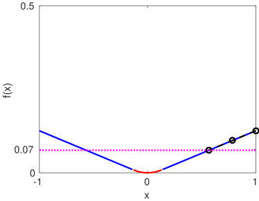
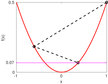
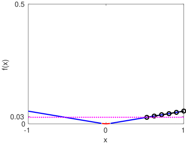
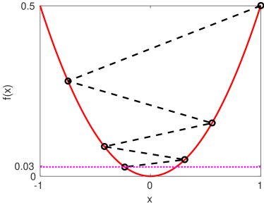
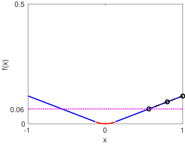
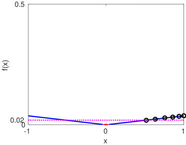
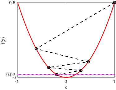
and a quadratic function $f_{\mathrm{2}}(\bm{x})$ (3.15), where $f_{\mathrm{1,GM}}(\bm{x};h,N)$ and $f_{\mathrm{2}}(\bm{x})$ contribute to the factors $\frac{1}{2Nh+1}$ and $(1-h)^{2N}$ respectively in (4.1). Here, $f_{\mathrm{1,GM}}(\bm{x};h,N)$ is a worst-case function where the GM iterates approach the optimum slowly, whereas $f_{\mathrm{2}}(\bm{x})$ is a worst-case function where the iterates overshoot the optimum. (See Fig. 1.)

Assuming that the above conjecture for a fixed-step GM holds, Taylor et al. taylor::ssc searched (numerically) for the optimal fixed-step size $0<h_{\mathrm{opt}}(N)<2$ for given $N$ that minimizes the bound (4.1):

$$h_{\mathrm{opt}}(N)\triangleq\mathop{\operator@font arg\,min}_{0<h<2}\max\left(\frac{1}{2Nh+1},(1-h)^{2N}\right).$$ (4.3)

GM with the step $h_{\mathrm{opt}}(N)$ has two worst-case functions $f_{\mathrm{1,GM}}(\bm{x};h,N)$ and $f_{\mathrm{2}}(\bm{x})$, and must compromise between two extreme cases. On the other hand, the case $0<h<h_{\mathrm{opt}}(N)$ has only $f_{\mathrm{1,GM}}(\bm{x};h,N)$ as the worst-case and the case $h_{\mathrm{opt}}(N)<h<2$ has only $f_{\mathrm{2}}(\bm{x})$ as the worst-case. We believe this compromise is inherent to optimizing the worst-case performance of FO methods. The next section shows that the optimal OGM also has this desirable property.

For the special case of $N=1$, the optimal OGM reduces to GM with a fixed-step $h=1.5$, and this confirms the conjecture in taylor::ssc that the step $h_{\mathrm{opt}}(1)=1.5$ (4.3) is optimal for a fixed-step GM with $N=1$. However, proving the optimality of $h_{\mathrm{opt}}(N)$ (4.3) for the fixed-step GM for $N>1$ is left as future work.

Fig. 1 visualizes the worst-case performance of GM with the optimal fixed-step $h_{\mathrm{opt}}(N)$ for $N=2$ and $N=5$. As discussed, for the two worst-case function in Fig. 1, the final iterates reach the same cost function value, where the iterates approach the optimum slowly for $f_{\mathrm{1,GM}}(\bm{x};h,N)$, and overshoot for $f_{\mathrm{2}}(\bm{x})$.

(a) $N=2$: $f_{\mathrm{1,GM}}\left(\bm{x};h_{\mathrm{opt}}(2),2\right)$

(b) $N=2$: $f_{\mathrm{2}}(\bm{x})$

(c) $N=5$: $f_{\mathrm{1,GM}}\left(\bm{x};h_{\mathrm{opt}}(5),5\right)$

(d) $N=5$: $f_{\mathrm{2}}(\bm{x})$

Figure 1: The worst-case performance of the sequence $\{\bm{x}_{i}\}_{i=0}^{N}$ of GM with an optimal fixed-step $h_{\mathrm{opt}}(N)$ for $N=2,5$ and $d=L=R=1$. The numerically optimized fixed-step sizes for $N=2,5$ are $h_{\mathrm{opt}}(2)=1.6058$ and $h_{\mathrm{opt}}(5)=1.7471$ taylor::ssc .

4.2 Two worst-case functions for the last iterate $\bm{x}_{N}$ of OGM

(kim::ofo, , Theorem 3) showed that $f_{\mathrm{1,OGM}}(\bm{x};N)$ (1.7) is a worst-case function for the last iterate $\bm{x}_{N}$ of OGM. The following theorem shows that a quadratic function $f_{\mathrm{2}}(\bm{x})$ (3.15) is also a worst-case function for the last iterate of OGM.

Theorem 4.1

For the quadratic function $f_{\mathrm{2}}(\bm{x})=\frac{L}{2}||\bm{x}||^{2}$ (3.15) in $\mathcal{F}_{L}(\mathbb{R}^{d})$, both OGM1 and OGM2 exactly achieve the convergence bound (1.5), i.e.,

$$f_{\mathrm{2}}(\bm{x}_{N})-f_{\mathrm{2}}(\bm{x}_{*})=\frac{LR^{2}}{2\theta_{N}^{2}}.$$

Proof

We use induction to show that the following iterates:

$$\bm{x}_{i}=(-1)^{i}\frac{1}{\theta_{i}}R\bm{\nu},\quad i=0,\ldots,N,$$ (4.4)

correspond to the iterates of OGM1 and OGM2 applied to $f_{\mathrm{2}}(\bm{x})$.

Starting from $\bm{x}_{0}=R\bm{\nu}$, where $\bm{\nu}$ is a unit vector, and assuming that (4.4) holds for $i<N$, we have

$$\bm{x}_{i+1} =\bm{x}_{i}-\frac{1}{L}\sum_{k=0}^{i}\hat{h}_{i+1,k}\nabla f_{\mathrm{2}}(\bm{x}_{k})$$

$$=\left(\bm{x}_{i}-\frac{1}{L}\hat{h}_{i+1,i}\nabla f_{\mathrm{2}}(\bm{x}_{i})\right)-\frac{1}{L}\sum_{k=0}^{i-1}\frac{\theta_{i}-1}{\theta_{i+1}}\hat{h}_{i,k}\nabla f_{\mathrm{2}}(\bm{x}_{k})+\frac{1}{L}\frac{\theta_{i}-1}{\theta_{i+1}}f_{\mathrm{2}}(\bm{x}_{i-1})$$

$$=\frac{1-2\theta_{i}}{\theta_{i+1}}\bm{x}_{i}+\frac{\theta_{i}-1}{\theta_{i+1}}(\bm{x}_{i}-\bm{x}_{i-1})+\frac{\theta_{i}-1}{\theta_{i+1}}\bm{x}_{i-1}=-\frac{\theta_{i}}{\theta_{i+1}}\bm{x}_{i}$$

$$=(-1)^{i+1}\frac{1}{\theta_{i+1}}R\bm{\nu},$$

where the second and third equalities use (1.1) and (2.5). Therefore, we have

$$f_{\mathrm{2}}(\bm{x}_{N})-f_{\mathrm{2}}(\bm{x}_{*})=f_{\mathrm{2}}\left((-1)^{N}\frac{1}{\theta_{N}}R\bm{\nu}\right)=\frac{LR^{2}}{2\theta_{N}^{2}}$$

after $N$ iterations of OGM1 and OGM2, exactly matching the bound (1.5). ∎

Thus the last iterate $\bm{x}_{N}$ of OGM has two worst case functions: $f_{\mathrm{1,OGM}}(\bm{x};N)$ and $f_{\mathrm{2}}(\bm{x})$, similar to an optimal fixed-step GM in Section 4.1. Fig. 2 illustrates behavior of OGM for $N=2$ and $N=5$, where OGM reaches same worst-case cost function value for two different functions $f_{\mathrm{1,OGM}}(\bm{x};N)$ and $f_{\mathrm{2}}(\bm{x})$ after $N$ iterations.

(a) $N=2$: $f_{\mathrm{1,OGM}}$ ($\bm{x}$;2)

(b) $N=2$: $f_{\mathrm{2}}(\bm{x})$

(c) $N=5$: $f_{\mathrm{1,OGM}}$ ($\bm{x}$;5)

(d) $N=5$: $f_{\mathrm{2}}(\bm{x})$

Figure 2: The worst-case performance of the secondary sequence $\{\bm{x}_{i}\}_{i=0}^{N}$ of OGM for $N=2,5$ and $d=L=R=1$.

In (taylor::ssc, , Conjecture 4) and Section 3.2, the primary sequence of OGM is conjectured to have $f_{\mathrm{1,OGM}^{\prime}}(\bm{x};N)$ as a worst-case function, whereas the quadratic function $f_{\mathrm{2}}(\bm{x})$ becomes the best-case as the first primary iterate of OGM reaches the optimum just in one step. On the other hand, Section 3.4 conjectured that $f_{\mathrm{2}}(\bm{x})$ is a worst-case function for the secondary sequence of OGM prior to the last iterate. Apparently the primary and secondary sequences of OGM have two extremely different worst-case analyses, whereas the last iterate $\bm{x}_{N}$ of OGM compromises between the two worst-case behaviors, making the worst-case behavior of the optimal OGM interesting.

5 Conclusion

We provided an analytical convergence bound for the primary sequence of OGM1 and OGM2, augmenting the bounds of the last iterate of the secondary sequence of OGM in kim::ofo . The corresponding convergence bound is twice as small as that of Nesterov’s FGM, showing that the primary sequence of OGM is faster than FGM. However, interestingly the intermediate iterates of the secondary sequence of OGM were found to be slower than FGM in the worst-case.

We proposed two new formulations of OGM, called OGM1^′ and OGM2^′ that are related closely to Nesterov’s accelerated first-order methods in nesterov:13:gmf (originally developed for nonsmooth composite convex functions and differing from FGM in nesterov:83:amf ; nesterov:05:smo ). For smooth problems, OGM and OGM^′ provide faster convergence speed than nesterov:13:gmf considering the number of gradient computations required per iteration.

We showed that the last iterate of the secondary sequence of OGM has two types of worst-case functions, a piecewise affine-quadratic function and a quadratic function. In light of the optimality of OGM (for $d\geq N+1$) in drori:16:tei , it is interesting that OGM has these two types of worst-case functions. Because the optimal fixed-step GM also appears to have two such worst-case functions, one might conjecture that this behavior is a general characteristic of optimal fixed-step first-order methods.

In addition to the optimality of fixed-step first-order methods for the cost function value, studying the optimality for an alternative criteria such as the gradient ($||\nabla f(\bm{x}_{N})||$) is an interesting research direction. Just as Nesterov’s FGM was extended for solving nonsmooth composite convex functions beck:09:afi ; nesterov:13:gmf , it would be interesting to extend OGM to such problems; recently this was numerically studied by Taylor et al. taylor:15:ewc . Incorporating a line-search scheme in beck:09:afi ; nesterov:13:gmf to OGM would be also worth investigating, since computing the Lipschitz constant $L$ is sometimes expensive in practice.

References

- (1) Beck, A., Teboulle, M.: A fast iterative shrinkage-thresholding algorithm for linear inverse problems. SIAM J. Imaging Sci. 2(1), 183–202 (2009). DOI 10.1137/080716542
- (2) Cevher, V., Becker, S., Schmidt, M.: Convex optimization for big data: scalable, randomized, and parallel algorithms for big data analytics. IEEE Sig. Proc. Mag. 31(5), 32–43 (2014). DOI 10.1109/MSP.2014.2329397
- (3) Drori, Y.: Contributions to the complexity analysis of optimization algorithms. Ph.D. thesis, Tel-Aviv Univ., Israel (2014)
- (4) Drori, Y.: The exact information-based complexity of smooth convex minimization (2016). URL http://arxiv.org/abs/1606.01424. Arxiv 1606.01424
- (5) Drori, Y., Teboulle, M.: Performance of first-order methods for smooth convex minimization: A novel approach. Math. Program. 145(1-2), 451–82 (2014). DOI 10.1007/s10107-013-0653-0
- (6) Drori, Y., Teboulle, M.: An optimal variant of Kelley’s cutting-plane method. Mathematical Programming (2016). DOI 10.1007/s10107-016-0985-7
- (7) Kim, D., Fessler, J.A.: Optimized first-order methods for smooth convex minimization. Mathematical Programming (2015). DOI 10.1007/s10107-015-0949-3
- (8) Lessard, L., Recht, B., Packard, A.: Analysis and design of optimization algorithms via integral quadratic constraints. SIAM J. Optim. 26(1), 57–95 (2016). DOI 10.1137/15M1009597
- (9) Nesterov, Y.: A method for unconstrained convex minimization problem with the rate of convergence . Dokl. Akad. Nauk. USSR 269(3), 543–7 (1983)
- (10) Nesterov, Y.: Introductory lectures on convex optimization: A basic course. Kluwer Academic Publishers, Dordrecht (2004)
- (11) Nesterov, Y.: Smooth minimization of non-smooth functions. Mathematical Programming 103(1), 127–52 (2005). DOI 10.1007/s10107-004-0552-5
- (12) Nesterov, Y.: Gradient methods for minimizing composite functions. Mathematical Programming 140(1), 125–61 (2013). DOI 10.1007/s10107-012-0629-5
- (13) Polyak, B.T.: Some methods of speeding up the convergence of iteration methods. USSR Comp. Math. Math. Phys. 4(5), 1–17 (1964)
- (14) Taylor, A.B., Hendrickx, J.M., Glineur, F.: Exact worst-case performance of first-order algorithms for composite convex optimization (2015). URL http://arxiv.org/abs/1512.07516. Arxiv 1512.07516
- (15) Taylor, A.B., Hendrickx, J.M., Glineur, F.: Smooth strongly convex interpolation and exact worst-case performance of first-order methods. Mathematical Programming (2016). DOI 10.1007/s10107-016-1009-3