A Smooth and Locally Sparse Estimator for Functional Linear Regression via Functional SCAD Penalty
Abstract
In this paper, we propose a new regularization technique called “functional SCAD”. We then combine this technique with the smoothing spline method to develop a smooth and locally sparse (i.e., zero on some sub-regions) estimator for the coefficient function in functional linear regression. The functional SCAD has a nice shrinkage property that enables our estimating procedure to identify the null subregions of the coefficient function without over shrinking the non-zero values of the coefficient function. Additionally, the smoothness of our estimated coefficient function is regularized by a roughness penalty rather than by controlling the number of knots. Our method is more theoretically sound and is computationally simpler than the other available methods. An asymptotic analysis shows that our estimator is consistent and can identify the null region with the probability tending to one. Furthermore, simulation studies show that our estimator has superior numerical performance. Finally, the practical merit of our method is demonstrated on two real applications.
1Department of Statistical Sciences, University of Toronto, Toronto, ON, Canada
2Department of Statistics and Actuarial Science, Simon Fraser University, Burnaby, BC, Canada
3Department of Statistics, Colorado State University, Fort Collins, CO, U.S.A.
keywords: B-spline basis, null region, smoothly clipped absolute deviation.
1 Introduction
In this paper, we study the problem of estimating the coefficient function in the following functional linear regression (FLR) model
| (1) |
where each is a scalar response, is the grand mean, are independent realizations of an unknown centered stochastic process defined on the domain , and , . The coefficient function is also called the regression weight function: weights the cumulative contribution of a functional predictor to the corresponding response . It is of practical interest to know where has no effect on , where has a significant effect on , and the effect magnitude. Statistically, this paper focuses on identifying the null subregions of (i.e., the subregions on which ), and simultaneously estimating on its non-null subregions.
Historically, functional linear regression originates from ordinary linear regression with a large number of predictors. When the number of predictors is very large, estimators produced by ordinary least squares exhibit excessive variability, and hence perform poorly on prediction. Researchers have developed many approaches to rectify the issue, such as partial least squares (PLS), principal components regression (PCR), and ridge regression, etc. Unfortunately, when the predictors were actually discrete observations of some continuous process, Hastie and Mallows, (1993) pointed out that none of these methods directly made use of the spatial information, i.e., the correlation and the order between predictors. They suggested that it would be more natural to regularize the variability by directly restricting the coefficient vector to be smooth. They also prototyped the ideas of penalized least squares and smoothing splines. These ideas were then explored more thoroughly in Ramsay and Silverman, (1997).
Following Hastie and Mallows, (1993) and Ramsay and Silverman, (1997), more theoretical and practical treatments of functional linear regression emerged. For example, Cardot et al., (2003) studied some theoretical aspects of FLR, such as identifiability, existence and unicity of the estimator of . They also proposed an estimator based on smoothing splines with a roughness penalty. The method developed by Crambes et al., (2009) is also based on smoothing splines, but it includes an unusual term in the roughness penalty to ensure the existence of their estimator without additional assumptions on sample curves. Both works used B-spline bases and provided convergence rates of the resulting estimators in terms of a norm induced by the covariance operator of the process . Instead of B-spline approximation, Li and Hsing, (2007) used a penalized Fourier basis to estimate , and derived an -norm convergence rate for their estimator. While Hastie and Mallows, (1993) motivated the aforementioned works to use penalized least squares, some researchers also used spectral decomposition of the covariance function of to estimate the coefficient function. For instance, Cardot et al., (2003) proposed to obtain an initial estimate through principal components regression and then smooth it by means of B-spline approximation. In Cai and Hall, (2006) and Hall and Horowitz, (2007), was estimated based on the spectral decomposition as well.
Besides the classic task of estimating , researchers have also studied some other aspects of FLR. For example, Cardot et al., (2007) investigated the convergence rates of some estimators in the weak topology of . Preda, (2007) and Yuan and Cai, (2010) explored FLR from the point of view of reproducing kernel Hilbert space. Müller and Stadtmüller, (2005) studied generalized functional linear models. Yao et al., (2005) extended the scope of FLR to the sparse longitudinal data. Fan and Zhang, (2000) and Lian, (2012) studied FLR with a functional response.
Recently, James et al., (2009) recognized the importance of the interpretability of estimated and proposed a so-called “FLiRTI” approach that intended to produce a more interpretable estimator. In order to obtain which is zero on subregions, FLiRTI penalizes the function values and derivatives at some grid points using the L1 regularization method. This method can successfully shrink small values of . Unfortunately, FLiRTI cannot warrant that the estimated is zero on some subregions for the following two reasons: 1) in order to have to be zero on some subregions, we need to force the function value at the group of grid points in those subregions to be zero simultaneously; 2) even we force a function and its first several derivatives to be zero at a point by L1 regularization, it may still nonzero at a subregion around the point: a smooth function is zero in a subregion around a point if and only if its value and all of its derivatives are zero at that point. As pointed out by Zhou et al., (2013), the FLiRTI estimate tends to have a large variation: a small grid size causes unstable numerical solution of the LASSO method; but a large set of dense grid points makes FLiRTI tend to overparametrize the model.
Zhou et al., (2013) also proposed a method for simultaneously identifying the null subregions of and estimating on its non-null subregions. The method has two stages: in the first stage, a Dantzig selector is used to obtain an initial estimate of the null subregions, and in the second stage, the estimated null subregions are refined. The estimate of on the non-null subregions is produced via a group SCAD penalty proposed by Wang et al., (2007). Selection of several tuning parameters in each stage not only increases the estimation variability and computational complexity but also makes the method difficult to implement, which limits the applications of this method.
In this paper, we first propose a new regularization technique called “functional SCAD” (fSCAD for short), and then combine it with smoothing splines to develop a one-stage procedure, called SLoS (Smooth and Locally Sparse). This procedure simultaneously identifies the null subregions of and produces a smooth estimate of in the non-null subregions. Here, “locally sparse” means a curve is zero on some subregions of its domain (Tu et al.,, 2012). The fSCAD can be viewed as a functional generalization of the ordinary SCAD proposed in Fan and Li, (2001). Its nice shrinkage property enables the SLoS estimating procedure to identify the null subregions of without over shrinking the non-zero values of on the non-null subregions. In addition, we employ a roughness penalty to regularize the smoothness of the SLoS estimator of . Compared to existing methods in the literature, our SLoS method has two distinct features. First, unlike the FLiRTI pointwise penalization method, our fSCAD regularizes the “overall magnitude” of the estimated coefficient function . Second, unlike the two-stage procedure in Zhou et al., (2013), our SLoS method combines fSCAD and smoothing splines together in a single optimization objective function. By solving this optimization problem, we are able to produce an estimate of the null subregions, as well as a smooth estimate of in its non-null subregions simultaneously in one single step. These two features make our estimating procedure theoretically sounder and computationally simpler.
The rest of the paper is organized as follows. In Section 2 we propose the fSCAD regularization technique and the SLoS estimator. In Section 2.1, we present the functional SCAD penalty and discuss its shrinkage property. We then provide a brief background of smoothing spline method in Section 2.2. In Section 2.3, we propose the SLoS estimator for the coefficient function . In Section 2.4, we extend our method to the case where there are multiple functional predictors. The asymptotic properties of the SLoS estimator are provided in Section 3. In Section 4 we evaluate the numerical performance of our estimator via simulation studies. In Section 5 we apply the SLoS method to study two real datasets. The paper is concluded in Section 6. Proofs of theorems are collected in a supplementary file. The Matlab codes for running the application and simulation studies can be downloaded at the website http://people.stat.sfu.ca/ cao/Research/FLR/.
2 Methodology
2.1 Functional SCAD
To motivate our functional SCAD, we first briefly review the ordinary SCAD penalty proposed by Fan and Li, (2001) in the setting of regression with multiple scalar predictors. Here, we use ordinary linear regression as an example to illustrate the SCAD technique. An ordinary linear model with one response variable and covariates can be expressed as
| (2) |
where . Using the least-squares function as a loss function, the SCAD estimator of is defined as
| (3) |
where the penalty function is the SCAD penalty function of Fan and Li, (2001). It is defined on as
where a suggested value for is according to Fan and Li, (2001), and is a tuning parameter varying with sample size. Additionally, when the number of covariates is fixed, the SCAD penalty enjoys the so-called oracle property: it is able to identify the true sub-model with probability tending to one, and meanwhile produce an asymptotically normal estimate for each non-zero variable (Fan and Li, (2001)). In other words, the estimator performs as well as if the true sub-model was known, i.e., we know which coefficients ’s are zero in advance. Even when the number of covariates grows as the sample size increases, still enjoys the oracle property under certain regularity conditions, as discussed in Fan and Peng, (2004) and Fan and Lv, (2011).
The ordinary linear model (2) changes to the functional linear model (1) if the summation is replaced by the integral . Similarly, for the SCAD penalty term in (3), if we normalize it by , then in the functional space, it is generalized to an integral . In this paper, we call
| (4) |
the fSCAD penalty.
We have introduced the fSCAD as an analogy to the ordinary SCAD. From that point of view, the fSCAD might be viewed as a functional generalization of the ordinary SCAD. Now, to gain insight into its shrinkage nature, we shall present a different way of introducing it in the setting of locally sparse modeling. For example, suppose is locally sparse and we want to have a locally sparse estimate of . A natural idea is to divide the domain into many small subintervals and then penalize the overall magnitude of on each subinterval to shrink the estimated towards zero on those subintervals where the true is zero. A possible measure of overall magnitude could be a normalized norm of on a subinterval, and a possible penalty function could be the ordinary SCAD penalty. The following remarkable result shows that this idea of locally sparse modeling actually leads to our fSCAD regularization.
Theorem 1.
Let be an equally spaced sequence in the domain , and denote the restriction of on the subinterval , i.e., for and zero elsewhere. If is continuous, then for any ,
| (5) |
where .
In Theorem 1, the normalized norm plays the role of measuring “overall magnitude” of over the subinterval . The identity (5) shows that, the fSCAD of is indeed the limit of the average SCAD penalty on the “overall magnitude” of over each small subinterval . This connection to the ordinary SCAD regularization sheds light on the shrinkage nature of fSCAD. Roughly speaking, with fSCAD regularization, Theorem 1 implies the following: 1) when is overall very small on (i.e., is very small), then the SCAD penalty will shrink towards zero identically over . This indicates that fSCAD is able to choose a locally sparse estimate; and 2) when has significant overall magnitude on (i.e., is big enough), then does not get penalized on the subinterval. This means fSCAD can avoid over shrinking .
Theorem 1 also provides a practical way to approximately compute the fSCAD penalty: we choose a large and then approximate by . When B-spline expansion (introduced in the next section) is used to approximate , we might take because it is relatively easy to compute the norm of a B-spline function. Moreover, for a B-spline basis, each only involves a few basis coefficients due to the compact support property of B-spline basis functions. In this particular setting, the approximated fSCAD can be viewed as a generalized SCAD with a diverging number of parameters.
The shrinkage feature of fSCAD brings it numerous potential applications in locally sparse modeling. For example, in Section 2.3, we use it to derive our SLoS estimator of the coefficient function in functional linear regression. Now we begin to discuss the shrinkage nature of the fSCAD in a more precise way. In other words, we will argue that the fSCAD shrinks the values of the estimator towards zero on the null subregions of , but does not over shrink the estimate on the non-null subregions. First of all, since
where denotes the supremum norm. Immediately, we have
| (6) |
Let denote and suppose is a consistent continuous estimator of . For any fixed , if , then by the continuity of we have on a small neighborhood of for some . When is sufficiently large, the subinterval containing is inside . Then with probability tending to one, we have for all and hence . As , with probability tending to one. This indicates that the consistent estimator does not get penalized for its values at . On the other hand, if on a small interval , then on with probability tending to one. When is sufficiently large, one or more subintervals are inside . Then in probability. By choosing an appropriate , the penalty grows with in the rate , and hence forces to become identically zero on .
2.2 Smoothing Spline Method
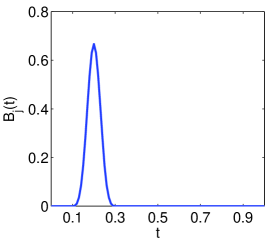
To prepare for the introduction of our SLoS estimator, in this section we briefly review the smoothing spline method for estimating . Recall that B-spline basis functions are defined by their order, as well as a sequence of knots. Suppose we set their order to and place equally spaced knots in the domain to define the B-spline basis functions. Over each subinterval, each B-spline basis function is a polynomial of the degree . Moreover, each B-spline basis function is nonzero over no more than consecutive subintervals. When is large, each B-spline basis function is only nonzero on a very short subregion. This property is called the compact support property, which is critical for efficient computation and makes B-spline bases very popular in functional data analysis. This property is also very important for us to practically compute the SLoS estimator. For example, Figure 1 shows one of 23 cubic B-spline basis functions defined with 21 equally spaced knots. This basis function is only nonzero on the interval [0.1,0.3]. Please refer to de Boor, (2001) for more details about B-spline basis functions.
Let denote the linear space spanned by the B-spline basis functions defined above. A modern method of estimating the coefficient function in the functional linear model (1) is to choose which minimizes the sum of squared residual errors. However, this method usually produces an estimator that exhibits excessive variability, especially when is relatively large. A popular approach to obtain a smooth estimator for is to add regularization through roughness penalty. For example, a smooth estimator of , proposed in Cardot et al., (2003), is defined as
where is the th order differential operator with , and denotes the norm of a function. The parameter is a tuning parameter varying with the sample size . Note that by setting , the above smooth estimator of is reduced to the classical ordinary least-squares estimator. This estimator is very rough when is large, while as , the estimator converges to a linear function. Thus, serves as a smoothing parameter, which controls the degree of smoothing of .
Although regularization via roughness penalty is able to produce a smooth estimator, it does not yield a locally sparse estimator. In other words, it is not able to identify the null subregions of . In the next section, we add the fSCAD to the fitting criterion to produce a smooth and meanwhile locally sparse estimate of .
2.3 The SLoS Estimator
We now combine fSCAD and smoothing splines together to obtain a smooth and locally sparse estimator for in the functional linear model (1), which is called the SLoS estimator in this paper.
The coefficient function along with the constant intercept is estimated by minimizing defined as follows:
| (7) |
where the minimization is taken over all and . In the fitting criterion, , we combine two penalty terms in a single optimization criterion: the roughness penalty regularizes the smoothness of , and the fSCAD penalty term regularizes the local sparseness of .
In the fitting criterion (7), we scale the fSCAD penalty up by the factor , where is the number of subintervals segmented by the knots of the B-spline basis functions for . This is necessary for the estimated coefficient function to enjoy the theoretical properties presented in Section 3. Also, according to Theorem 1, the fSCAD penalty term can be approximated by
| (8) |
Thus, the fSCAD penalty term actually represents the penalty on the overall magnitude of of all subintervals. Based on this observation, we emphasize that the fSCAD penalty regularizes in the way that it penalizes the overall magnitude of on each subinterval, rather than the pointwise penalization fashion adopted in FLiRTI (James et al.,, 2009). This ensures that if the fSCAD regularization forces the overall magnitude of on a subinterval to be zero, then the estimated is identically zero almost everywhere on that subinterval. Therefore, our method overcomes the shortcoming of the FLiRTI (James et al.,, 2009). Moreover, our one-stage fitting procedure is computationally simpler than the two-stage method proposed by Zhou et al., (2013).
Below we shall show how to compute the SLoS estimator in practice. To simplify the notation and manifest our main idea, we assume , and redefine the function . The case that is considered at the end of this section. We estimate as a linear combination of B-spline basis functions:
where is the vector of B-spline basis functions, and is the corresponding vector of coefficients. Let be an matrix with entries for , . Let . Then the first term of in (7) is expressed in the matrix notation as
| (9) |
Let be an matrix with entries for . Then the second term of in (7) is
| (10) |
Next, we turn to the third term of in (7). According to Theorem 1, we approximate the fSCAD penalty term as (8), and
where is an -by- matrix with entries if and zero otherwise. The SCAD penalty function might be approximated by the local quadratic approximation (LQA) proposed in Fan and Li, (2001) as follows, since it makes the computation simpler. When , the LQA of SCAD function is
Then given some initial estimate , for we have
| (11) |
where is a term defined as
Let
| (12) |
Then we have
| (13) |
Now, we put (9), (10) and (13) together to express in the matrix notation as
| (14) |
Thus, optimizing with respect to is equivalent to optimizing with respect to in (14). Also note that the term does not depend on and hence has no impact on optimizing . Differentiating with respect to and setting it to zero, we have the following equation
with the solution
As in Fan and Li, (2001), we repeat the above computation steps until converges and in each iteration we manually shrink variables that are very small to zero. In summary, we have the following algorithm to compute and obtain the estimator :
-
Compute the initial estimate ;
-
Given , compute and ; if a variable is very small in magnitude and makes almost singular or badly scaled so that inverting is numerically unstable, then it is manually shrunk to zero;
-
Repeat Step 2 until the convergence of is reached.
To carry out the above algorithm, we need to evaluate the matrix with elements . When covariate functions are not fully observed, approximation of elements is mandatory. Provided that covariate functions are observed at a regular and dense grid of time points over , we can compute . An alternative approach is to fit each using the spline regression method first. Then we compute , where is the fitted curve of based on the observations . When the grid is regular and dense, these two approaches yield an almost identical approximate of . When is observed on a sparse and irregular grid, we can first estimate from the sparse measurements using some available methods such as functional principal component analysis (Yao et al. (2005)).
When , we modify the matrices , and as follows to produce an estimate of simultaneously: 1) add one more parameter to the topmost of the column vector ; 2) add one more column of all ones to the leftmost of ; 3) add one column of all zeros to the leftmost of both and , and then add one more row of all zeros to the topmost of both and . With these changes, the algorithm above can be carried out to estimate and simultaneously.
When using the smoothing spline method, the choice of is not crucial (Cardot et al., (2003)), as the roughness of the estimator is controlled by the roughness penalty, rather than the number of knots. This is demonstrated by a simulation study, which is detailed in Section A in the supplementary file. The simulation study also provides a practical guideline on choosing : estimators with a larger perform better in identifying null region of , while those with a smaller perform better in prediction. Once is determined, we can perform a search over a grid of candidate values of and based on some popular selection criteria such as cross-validation, generalized cross-validation, BIC, AIC or RIC.
2.4 Extension to Multiple Regressors
Our method can also be extended to estimate the following functional linear model with multiple functional covariates:
| (15) |
where each is a scalar response, is the grand mean, are independent realizations of an unknown centered stochastic process defined on the domain , and , . We estimate the coefficient functions, , and by minimizing
| (16) |
where . The computational steps described in Section (2.3) are modified as follows to minimize . Corresponding to each regressor , we compute the matrix , which has entries for , . Let be the column catenation of , and correspondingly set , i.e., set to be the matrix with blocks in its main diagonal and zeros elsewhere. For each , we also have a matrix which corresponds to the matrix in (12). Then in (14) is replaced by . After these modifications, the iterative algorithm described in Section 2.3 can be carried out without any change.
3 Theoretical Properties
Let us set up some notations first. We use to denote the empirical version of the covariance operator of the random process , and is defined by
For a function , define a semi-norm and its population version . Let denote the null region of and denote the non-null region of , i.e., and .
We also assume the following regularity conditions:
-
(C1)
is almost surely bounded, i.e., a.s for some constant . Here, denotes .
-
(C2)
is in the Hölder space . That is, for some constant , integer and . Let . Assume , where is the degree of the B-spline basis.
-
(C3)
There exists a sequence of such that , such that , and .
In the above, (C1) and (C2) are the same as (H1) and (H3) of Cardot et al., (2003). Additionally, Assumption (C3) is analogous to regularity conditions () and () in Fan and Peng, (2004) to ensure the unbiasedness and guarantee that the penalty does not dominate the least squares. Intuitively, Assumption (C3) prevents the tail of on its support from being too thin. If the tail is too thin, then the fSCAD penalty dominates the least squares loss.
Recall that and are tuning parameter varying with . To emphasize their dependency on the sample size , we denote them by and , respectively. In addition, we assume the following conditions on choosing values of , and :
-
(C4)
and .
The theorem below establishes the existence of our estimator and its consistency.
Theorem 2.
Under assumptions (C1)-(C4), with probability tending to one, there exists a local minimizer of (7) such that and .
We now introduce some notations for stating the next property. First, recall that the support of is defined as the closure of . For any and a subset of the real line , the -neighborhood of , defined by , is denoted by . We also define as . Intuitively, extends a little bit, while shrinks a little bit. The following theorem shows that, with probability tending to one, is collectively zero on the null region except for those points on the boundaries.
Theorem 3.
Under conditions (C1)-(C4), as , For every not in the support of , we have with probability tending to one. Moreover, for every , we have and with probability tending to one, where denotes the interior of .
Proofs of the above theorem have been relegated to supplementary file.
4 Simulation Studies
We conducted a simulation study to investigate the numerical performance of our SLoS estimator. In this study, we compared our estimator to the following estimators: 1) the ordinary least squares (OLS) estimator, corresponding to and , 2) the smoothing spline (Smooth) estimator proposed in Cardot et al., (2003), corresponding to , and 3) the oracle estimator. The oracle estimator was computed by placing equally spaced knots only on the non-null region and was regularized by a roughness penalty. Notice that only the oracle estimator assumes the null region is known, while the other three estimators do not know the null region. It will be shown that our SLoS estimator performs much better than the OLS estimator and the smooth estimator, and the SLoS estimator performs almost as well as the oracle estimator, although our SLoS estimator does not know the null region in advance. In our simulation study, we did not compare our method with Zhou et al., (2013) and James et al., (2009) because, the FLiRTI method proposed in James et al., (2009) is numerically unstable in our simulation settings, and the method of Zhou et al., (2013) is fairly difficult to implement and tune. This difficulty stems from the fact that, at each stage, several tuning parameters have to be chosen carefully.
In the comparison, we reported the integrated squared error () defined on the null region and the non-null region as follows
| (17) |
where was the length of the null region and was the length of the non-null region of . and measure the integrated squared error between an estimated coefficient function and the true function on the null region and the non-null region, respectively. We also assessed the performance of estimators on prediction by the mean squared error (MSE) on predicting on a test dataset that is independent of the training dataset. The prediction mean sqaured error () is computed as follows:
| (18) |
where denotes the test dataset, is the size of the test dataset, and is the estimated intercept and coefficient function from the training dataset.
The SLoS estimator used cubic B-spline basis functions defined by equally spaced knots in [0,1]. For choosing , we found that the empirical formula works quite well in practice, where denotes the integer closest to . According to this formula, . It made large enough to well approximate the fSCAD penalty. The values of in the following simulation studies were determined by the above formula. The tuning parameters and were chosen using BIC as the selection criterion by the procedure proposed in Section 2.3. BIC was used because it encouraged sparser models. The smoothing spline method also used cubic B-spline basis functions, and used AIC to choose the smoothing parameter and the number of knots that defined the B-spline basis, because AIC yielded better performance than cross-validation or BIC. The OLS estimator also used AIC to choose the order and the number of knots which defined the B-spline basis, because AIC also yielded better performance than cross-validation or BIC. The oracle estimator used cross-validation to choose the number of knots and the smoothing parameter , as cross-validation yielded better performance than AIC or BIC.
We considered the functional linear model
| (19) |
where . Three different types of coefficient functions were considered:
-
Case I:
There is no signal, i.e., .
-
Case II:
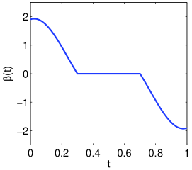
There is a flat region of . We considered the following function
which vanishes on . The function is plotted in Figure 2LABEL:sub@subfig:case-II.
-
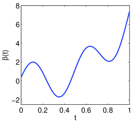
Case III:
There is no flat region of . We considered . It is plotted in Figure 2LABEL:sub@subfig:case-III. It was designed so that it has no flat region, but crosses zero twice. Therefore, this case does not favor the SLoS method.
The measurement error was set to 1 in Case I, and chosen so that the signal-to-noise ratio equals to 4 in the other two cases. The true was set to 1.
The covariate functions were generated based on the equation , where the coefficients were generated from the standard normal distribution, and were B-spline basis functions defined by order 5 and 71 equally spaced knots (the number 71 is randomly selected between 50 and 100). Using this model, for each sample size , we independently generated 100 datasets. For each dataset, we also generated a separate test dataset with the sample size 5000.
| Oracle | OLS | Smooth | SLoS | |||||
|---|---|---|---|---|---|---|---|---|
| Case I | ||||||||
| - | 2. | 10 (1.61) | 0. | 91 (0.92) | 0. | 23 (0.43) | ||
| - | 0. | 57 (0.46) | 0. | 29 (0.24) | 0. | 05 (0.11) | ||
| - | 0. | 27 (0.22) | 0. | 12 (0.10) | 0. | 02 (0.03) | ||
| Case II | ||||||||
| 1. | 62 (0.89) | 3. | 89 (2.39) | 3. | 47 (2.18) | 2. | 11 (1.25) | |
| 0. | 58 (0.32) | 1. | 28 (0.58) | 1. | 06 (0.40) | 0. | 72 (0.36) | |
| 0. | 28 (0.14) | 0. | 67 (0.31) | 0. | 57 (0.24) | 0. | 37 (0.16) | |
| Case III | ||||||||
| - | 2. | 25 (1.42) | 2. | 12 (1.36) | 1. | 83 (0.78) | ||
| - | 0. | 64 (0.35) | 0. | 61 (0.28) | 0. | 56 (0.21) | ||
| - | 0. | 35 (0.20) | 0. | 30 (0.15) | 0. | 28 (0.11) | ||
| OLS | Smooth | SLoS | |||
|---|---|---|---|---|---|
| Case I | |||||
| 1.65 (1.67) | 0. | 57 (0.72) | 0. | 06 (0.31) | |
| 0.42 (0.41) | 0. | 18 (0.18) | 0. | 01 (0.10) | |
| 0.20 (0.22) | 0. | 08 (0.08) | 0. | 00 (0.00) | |
| Case II | |||||
| 19.75 (18.15) | 20. | 09 (18.20) | 0. | 15 (0.32) | |
| 7.34 (4.62) | 6. | 37 (3.31) | 0. | 04 (0.09) | |
| 4.23 (3.10) | 4. | 00 (2.58) | 0. | 01 (0.03) | |
| Oracle | OLS | Smooth | SLoS | |||||
|---|---|---|---|---|---|---|---|---|
| Case II | ||||||||
| 1. | 93 (1.18) | 4. | 13 (3.56) | 3. | 11 (2.68) | 2. | 51 (1.60) | |
| 0. | 73 (0.44) | 1. | 23 (0.88) | 0. | 88 (0.47) | 0. | 86 (0.44) | |
| 0. | 37 (0.18) | 0. | 66 (0.39) | 0. | 46 (0.22) | 0. | 46 (0.19) | |
| Case III | ||||||||
| - | 1. | 88 (1.55) | 1. | 64 (1.35) | 1. | 32 (0.61) | ||
| - | 0. | 52 (0.36) | 0. | 46 (0.25) | 0. | 41 (0.17) | ||
| - | 0. | 28 (0.20) | 0. | 22 (0.12) | 0. | 20 (0.08) | ||
The simulation results are shown in Table 1, 2 and 3. They clearly show that the SLoS method wins under each evaluation criterion in all cases except the oracle procedure. From Table 1, we can see that, in terms of prediction, our method performs significantly better than the OLS and Smooth estimators in Case I and II. Surprisingly, it also performs slightly better than the other two methods in Case III, although this case does not favor the SLoS estimator. We investigated this phenomenon, and found that the shrinkage effect of fSCAD penalty reduced the variability of SLoS estimator without causing significant bias. The reduction of variability is more significant when sample size is small. Therefore, our estimator yielded a better variance-bias tradeoff on the performance of prediction. We also noticed that the oracle procedure only performed slightly better than the SLoS method.
In terms of estimation of , Table 2 shows that the SLoS method yielded a much lower integrated squared error on the null region, and Table 3 shows that it has a similar performance to the Smooth estimator on the non-null region. Even in Case III where the setting does not favor the SLoS method, the SLoS estimator still slightly outperforms the OLS and Smooth estimators. In summary, the SLoS method stands out in both predicting response variable and estimating the coefficient function .
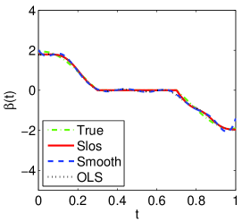
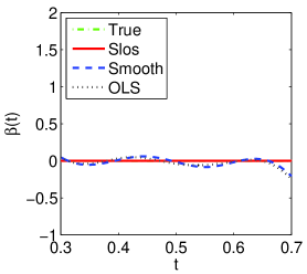
We also evaluate the ability of SLoS method to identify the null subregions. Figure 3LABEL:sub@subfig:rand-s1 displays the estimated by SLoS, OLS and Smooth method in one random simulation replicate, as well as the true . The estimated by the oracle procedure is not displayed in Figure 3LABEL:sub@subfig:rand-s1, as it is almost identical to the true and is hard to be distinguished in the graph. Figure 3LABEL:sub@subfig:rand-s1 shows that all three methods produce a very good estimate of . To get a close look at the null sug-region, Figure 3LABEL:sub@subfig:rand-s1-n1 displays the same functions of Figure 3LABEL:sub@subfig:rand-s1 only in the null region . In this figure, we can see that, for the SLoS estimator, it is identically zero. However, the estimated produced by the other two methods are non-zero almost everywhere in the null region . We also observe similar results in most of other simulation replicates.
Finally, we quantify the ability to identify the null subregions using the average of proportions of null subregions that are correctly identified by the SLoS estimator, which is computed as follows. First, for each run, we compute the value of on a sequence of dense and equally-spaced points in the null subregion. For example, in Case I, the sequence is taken to be , and in Case II, it is taken to be . Then we compute the proportion of the points at which is zero among all points in the sequence. Finally, we average the calculated proportions from 100 runs. The result is summarized in Table 4. It shows that the performance of our estimator on identifying null region is quite remarkable: in Case I (Case II, respectively), on average more than 95% (92%) of the null region was correctly identified when , and this number increases to 100% (95%) when . This also numerically verifies the conclusion in Theorem 3.
| Case I (%) | 98.40 (6.14) | 99.70 (1.75) | 100 (0.00) |
| Case II (%) | 92.20 (5.47) | 93.41 (3.27) | 95.01 (2.04) |
5 Applications
5.1 Canadian Weather Data
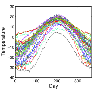
Ramsay and Silverman, (2005) studied the relationship between the daily mean temperature curves and the annual rainfall by analyzing the weather data of 35 Canadian cities. This relationship is modelled using the functional linear regression model (1), where the daily mean temperature curve is the functional covariate, and the logarithm of the annual rainfall is the response variable. Figure 4 displays the daily mean temperature recorded at 35 Canadian cities in one year.
We applied our SLoS approach to estimate the functional linear regression model (1) from the Canadian weather data. The coefficient function was estimated as a linear combination of cubic B-spline basis functions defined on with . Here, the value of was also set by the empirical formula that is introduced in the previous section. To respect the periodic nature of temperature cycles, we restricted that . The tuning parameters were chosen by the the procedure proposed in Section 2.3.
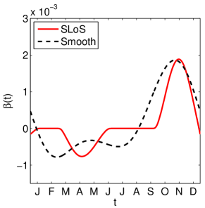
Figure 5 shows the temperature coefficient function estimated by our SLoS method and the smoothing spline method (Cardot et al.,, 2003). It shows that the estimated coefficient function is zero roughly in January and summer months (late June, July, August and early September). This suggests the temperature in summer has no significant effect on the annual rainfall. Our method also produced a smooth estimate of on the non-null subregions. It indicates that the temperature in fall months (late October, November and early December) has a significant contribution to the annual rainfall. These results are consistent with the results discovered in the previous research on this data (James et al.,, 2009).
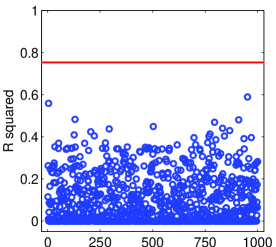
Figure 6 shows the results of a permutation test for SLoS estimator on this data. The solid line represents the for the SLoS estimator, which is 0.73. The responses are random permuted 1000 times and the new are plotted in Figure 6, indicated by circles. All 1000 permuted are under 0.73. This provides strong evidence of the relationship between temperature and annual rainfall discovered by our SLoS method.
5.2 Spectrometric Data
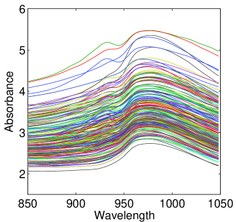
The data is available at http://www.math.univ-toulouse.fr/ferraty/SOFTWARES/NPFDA/npfda-datasets.html, which originates from Tecator dataset (http://lib.stat.cmu.edu/datasets/tecator). There are in total 215 samples. Each sample contains finely chopped pure meat, and a spectrometric curve of spectra of absorbances measured at 100 wavelengths among 850 - 1050 nm is recorded. Figure 7 displays the 215 curves in the dataset. At the same time, the fat content, measured in percent, is also determined by analytic chemistry. The task is to predict the fat content based on the spectrometric curve. Our interest is to investigate what range of spectra that has predicting power on fat content and what range that does not.
We applied our SLoS approach to estimate the functional linear regression model (1) from the spectrometric data. The coefficient function was estimated as a linear combination of cubic B-spline basis functions defined on with . Here, the value of was also set by the empirical formula that is introduced in the previous section. The tuning parameters were chosen by the the procedure proposed in Section 2.3.
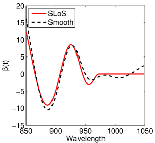
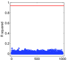
Figure 8 shows the coefficient function estimated by our SLoS method and the smoothing spline method (Cardot et al.,, 2003). It shows that the estimated coefficient function is zero roughly on [970,1050]. This suggests the high end of spectrum has no predicting power on fat content. Our method also produced a smooth estimate of on the non-null subregions. It indicates spectrum channels with wavelength among 850 - 970 nm have a significant contribution to the prediction power of the fat content. Figure 9 shows the results of a permutation test for SLoS estimator on this data. The solid line represents the for the SLoS estimator, which is 0.94. The responses are randomly permuted 1000 times and the new are plotted in Figure 9, indicated by circles. All 1000 permuted are under 0.2. This provides strong evidence of the relationship between spectrum and fat content discovered by our SLoS method.
6 Concluding Remarks
When a large number of predictors are involved in a regression problem, parsimonious models via SCAD or other shrinkage regularization methods have been proven to have less variability and better interpretability. In this paper, we propose the functional SCAD regularization method which extends the ordinary SCAD to the functional setting. The functional SCAD, when combined with the penalized B-spline expansion method, yields a smooth and locally sparse (SLoS) estimator of the coefficient function in functional linear regression.
The SLoS procedure is a combination of three techniques: 1) the functional SCAD that is responsible for identifying the null subregions of the coefficient function while at the same time avoiding over shrinking the non-zero values, 2) the B-spline basis expansion that is used to practically compute the SLoS estimator efficiently thanks to its compact support property, and 3) the roughness regularization that assures the smoothness of our estimator even when a large number of knots are used to define the B-spline basis. Therefore, our method is able to accurately identify the null region and simultaneously produce a smooth estimator on the non-null region. Comparing to existing methods in the literature, our estimation procedure is more theoretically sound and is computationally simpler. The simulation studies show that our estimator has superior numerical performance and finite-sample properties. Furthermore, the applications on two real datasets demonstrate the practical merit of our method.
In summary, while our work focused on the functional linear regression, it is important to recognize that the functional SCAD is in fact a very general regularization technique which can be applied in many other domains in functional data analysis. For example, it may be used in a spline smoothing problem to obtain a smooth and locally sparse estimator of an unknown curve. It can also be used in functional principle component analysis to produce smooth and locally sparse functional principal components. Both of these problems are suggested starting points for future research.
References
- Cai and Hall, (2006) Cai, T. T. and Hall, P. (2006). Prediction in functional linear regression. The Annals of Statistics, 34(5):2159–2179.
- Cardot et al., (2003) Cardot, H., Ferraty, F., and Sarda, P. (2003). Spline estimators for the functional linear model. Statistica Sinica, 13:571–591.
- Cardot et al., (2007) Cardot, H., Mas, A., and Sarda, P. (2007). CLT in functional linear regression models. Probability Theory and Related Fields, 138:325–361.
- Crambes et al., (2009) Crambes, C., Kneip, A., and Sarda, P. (2009). Smoothing splines estimators for functional linear regression. The Annals of Statistics, 37(1):35–72.
- de Boor, (2001) de Boor, C. (2001). A practical Guide to Splines. Springer-Verlag, New York.
- Fan and Li, (2001) Fan, J. and Li, R. (2001). Variable selection via nonconcave penalized likelihood and its oracle properties. Journal of the American Statistical Association, 96(456):1348–1360.
- Fan and Lv, (2011) Fan, J. and Lv, J. (2011). Non-concave penalized likelihood with NP-dimensionality. IEEE Transactions on Information Theory, 57:5467–5484.
- Fan and Peng, (2004) Fan, J. and Peng, H. (2004). Nonconcave penalized likelihood with a diverging number of parameters. The Annals of Statistics, 32(3):928–961.
- Fan and Zhang, (2000) Fan, J. and Zhang, J.-T. (2000). Two-step estimation of functional linear models with applications to longitudinal data. Journal of the Royal Statistical Society. Series B (Statistical Methodology), 62(2):303–322.
- Hall and Horowitz, (2007) Hall, P. and Horowitz, J. L. (2007). Methodology and convergence rates for functional linear regression. The Annals of Statistics, 35(1):70–91.
- Hastie and Mallows, (1993) Hastie, T. and Mallows, C. (1993). A statistical view of some chemometrics regression tools]: Discussion. Technometrics, 35(2):140–143.
- James et al., (2009) James, G. M., Wang, J., and Zhu, J. (2009). Functional linear regression that’s interpretable. The Annals of Statistics, 37(5A):2083–2108.
- Li and Hsing, (2007) Li, Y. and Hsing, T. (2007). On rates of convergence in functional linear regression. Journal of Multivariate Analysis, 98:1782–1804.
- Lian, (2012) Lian, H. (2012). Convergence of nonparametric functional regression estimates with functional responses. Electronic Journal of Statistics, 6:1373–1391.
- Müller and Stadtmüller, (2005) Müller, H.-G. and Stadtmüller, U. (2005). Generalized functional linear models. The Annals of Statistics, 33(2):774–805.
- Preda, (2007) Preda, C. (2007). Regression models for functional data by reproducing kernel Hilbert spaces methods. Journal of Statistical Planning and Inference, 137:829–840.
- Ramsay and Silverman, (1997) Ramsay, J. O. and Silverman, B. W. (1997). Functional Data Analysis. Springer-Verlag, New York.
- Ramsay and Silverman, (2005) Ramsay, J. O. and Silverman, B. W. (2005). Functional Data Analysis. Springer Series in Statistics. Springer, 2nd edition.
- Tu et al., (2012) Tu, C. Y., Song, D., Breidt, F. J., Berger, T. W., and Wang, H. (2012). Functional model selection for sparse binary time series with multiple inputs. Economic Time Series: Modeling and Seasonality, pages 477–497.
- Wang et al., (2007) Wang, L., Chen, G., , and Li, H. (2007). Group scad regression analysis for microarray time course gene expression data. Bioinformatics, 23(12):1486–1494.
- Yao et al., (2005) Yao, F., Müller, H.-G., and Wang, J.-L. (2005). Functional linear regression analysis for longitudinal data. The Annals of Statistics, 33(6):2873–2903.
- Yuan and Cai, (2010) Yuan, M. and Cai, T. T. (2010). A reproducing kernel Hilbert space approach to functional linear regression. The Annals of Statistics, 38(6):3412–3444.
- Zhou et al., (2013) Zhou, J., Wang, N.-Y., and Wang, N. (2013). Functional linear model with zero-value coefficient function at sub-regions. Statistica Sinica, 23:25–50.