The VMC Survey - XX. Identification of new Cepheids in the Small Magellanic Cloud

Abstract

We present $K_{\mathrm{s}}$-band light curves for 299 Cepheids in the Small Magellanic Cloud (SMC) of which 288 are new discoveries that we have identified using multi-epoch near-infrared photometry obtained by the VISTA survey of the Magellanic Clouds system (VMC). The new Cepheids have periods in the range from 0.34 to 9.1 days and cover the magnitude interval 12.9 $\leq\langle K_{\mathrm{s}}\rangle\leq$ 17.6 mag. Our method was developed using variable stars previously identified by the optical microlensing survey OGLE. We focus on searching new Cepheids in external regions of the SMC for which complete VMC $K_{\mathrm{s}}$-band observations are available and no comprehensive identification of different types of variable stars from other surveys exists yet.

1 Introduction

The Visual and Infrared survey Telescope for Astronomy (VISTA, Emerson et al. 2006) survey of the Magellanic Clouds system (VMC, Cioni et al. 2011) is collecting $Y,J,K_{\mathrm{s}}$ photometry down to $Y$=21.9 mag, $J$=22.0 mag, $K_{\mathrm{s}}$=21.5 mag (5 $\sigma$ level on the stacked images) for sources in the Large Magellanic Cloud (LMC), the Small Magellanic Cloud (SMC), the Bridge connecting them, and a small part of the Magellanic Stream. The VMC images are processed by the Cambridge Astronomical Survey Unit (CASU; Lewis et al. 2010) through the VISTA Data Flow System (VDFS) pipeline that performs aperture photometry of the images. The reduced data are then further processed by the Wide Field Astronomy Unit (WFAU) in Edinburgh where the single epochs are stacked and catalogued in the VISTA Science Archive (VSA; Cross et al. 2012). As of 2016 January, the VMC survey observations are 74% complete, with specific completion levels of 62%, 95%, 95% and 100% for the LMC, the SMC, the Bridge and the Stream, respectively. A main aim of the VMC survey is to study the structure of the whole Magellanic system using different distance indicators. Among them, most notably, are primary standard candles such as the Cepheids and the RR Lyrae stars, for which VMC is obtaining $K_{\mathrm{s}}$-band light curves with 13 (or more) individual epochs, with most epochs reaching a depth of $K_{\mathrm{s}}$=19.3 mag (5 $\sigma$ level). The significantly reduced amplitude of these pulsating variables in the near-infrared, with respect to the optical bands, along with the multi-epoch cadence of the VMC $K_{\mathrm{s}}$-band observations, allows us to infer accurate mean $K_{\mathrm{s}}$ magnitudes. Furthermore, the near-infrared period-luminosity ($PL$) relations are intrinsically much narrower than the corresponding optical relations and less affected by systematic uncertainties in reddening and metal content (Caputo et al., 2000). For these reasons the VMC data are very well suited to construct $PL$ relations with a high level of precision and accuracy (e.g. Ripepi et al. 2012a, b, 2014, 2015; Muraveva et al. 2015). Conversely, the smaller amplitudes compared to optical bands make it more difficult to identify these variables from near-infrared data alone. In VMC, most of the information (identification, period, variability type, etc.) needed to fold the $Y,J,K_{\mathrm{s}}$-band light curves and derive average $Y,J,K_{\mathrm{s}}$ magnitudes for the variable stars are taken from the catalogues of Magellanic Cloud variables produced by large microlensing optical surveys such as MACHO (Alcock et al., 2000), EROS (Tisserand et al., 2007) and OGLE (Soszyński et al., 2008a) that were conducted in the last two decades to search for baryonic dark matter in the Milky Way. As described in Udalski et al. (2015), the observations of the fourth phase of the OGLE project (hereinafter, OGLE IV) have been successfully run over the last five years. First results have been published in Soszyński et al. (2012) (South Ecliptic Pole region), Kozłowski et al. (2013) (Magellanic Bridge) and Soszyński et al. (2015a) (anomalous Cepheids).

Table 1: Information on the $K_{\mathrm{s}}$-band photometry of the VMC tiles analyzed in this paper. Col. 1: Field and tile number, Col. 2: Right Ascension (RA, J2000), Col. 3: Declination (Dec, J2000), Col. 4: position angle, Col. 5: number of $K_{\mathrm{s}}$ observations, Cols. 6,7: Dates of the 1st and last observations expressed in dd/mm/yy format, Col. 8: Time interval (T.I.) between first and last observations, Col. 9: Airmass, Col. 10: Full Width at Half Maximum (FWHM), Col. 11: Ellipticity, Col. 12: Limiting magnitude. Reported values of airmass, FWHM, ellipticity and limiting magnitude are averages over all nights. They are indicated with their respective standard deviations. The number of epochs ($N_{K_{\mathrm{s}}}$) includes both shallow and deep observations (see text for details).

$$\begin{array}[]{cccccccrcccc}\hline\cr\hline\cr\vskip 3.0pt plus 1.0pt minus 1.0pt\cr\mathrm{Tile}&\alpha&\delta&\mathrm{\phi}&N_{K_{\mathrm{s}}}&\mathrm{1st\,Epoch}&\mathrm{Last\,Epoch}&\mathrm{T.\,I.}&\mathrm{Airmass}&\mathrm{FWHM}&e&\mathrm{LimMag}\\ &\mathrm{(h:m:s)}&(^{\circ}\mathrm{:}^{\prime}\mathrm{:}^{\prime\prime})&\mathrm{(deg)}&&&&\mathrm{(d)}&&&&\mathrm{(mag)}\\ \vskip 3.0pt plus 1.0pt minus 1.0pt\cr\hline\cr\vskip 3.0pt plus 1.0pt minus 1.0pt\cr\mathrm{LMC\,6\_8}&06\mathrm{:}02\mathrm{:}21.984&-69\mathrm{:}14\mathrm{:}42.360&-83.7904&15&23/02/11&16/04/14&1148&1.49\pm 0.04&0.96\pm 0.19&0.06\pm 0.01&19.30\pm 0.24\\ \vskip 3.0pt plus 1.0pt minus 1.0pt\cr\mathrm{LMC\,7\_3}&05\mathrm{:}02\mathrm{:}55.200&-67\mathrm{:}42\mathrm{:}14.760&-97.7044&16&12/01/11&04/03/13&782&1.44\pm 0.05&0.95\pm 0.10&0.06\pm 0.02&19.23\pm 0.19\\ \vskip 3.0pt plus 1.0pt minus 1.0pt\cr\mathrm{LMC\,8\_8}&05\mathrm{:}59\mathrm{:}23.136&-66\mathrm{:}20\mathrm{:}28.680&-84.4802&16&14/11/09&26/11/10&377&1.39\pm 0.05&0.93\pm 0.11&0.06\pm 0.02&19.36\pm 0.27\\ \vskip 3.0pt plus 1.0pt minus 1.0pt\cr&&&&&&&&&&&\\ \mathrm{SMC\,3\_1}&00\mathrm{:}02\mathrm{:}39.912&-73\mathrm{:}53\mathrm{:}31.920&-11.3123&16&21/08/12&01/07/14&679&1.60\pm 0.05&1.01\pm 0.15&0.05\pm 0.01&19.38\pm 0.16\\ \vskip 3.0pt plus 1.0pt minus 1.0pt\cr\mathrm{SMC\,3\_3}&00\mathrm{:}44\mathrm{:}55.896&-74\mathrm{:}12\mathrm{:}42.120&-1.2120&18&03/08/11&05/09/12&399&1.62\pm 0.04&1.02\pm 0.10&0.07\pm 0.02&19.35\pm 0.15\\ \vskip 3.0pt plus 1.0pt minus 1.0pt\cr\mathrm{SMC\,3\_5}&01\mathrm{:}27\mathrm{:}30.816&-74\mathrm{:}00\mathrm{:}49.320&+8.9671&16&29/07/11&07/10/12&436&1.58\pm 0.06&1.02\pm 0.15&0.06\pm 0.01&19.34\pm 0.22\\ \vskip 3.0pt plus 1.0pt minus 1.0pt\cr\mathrm{SMC\,4\_2}&00\mathrm{:}25\mathrm{:}14.088&-73\mathrm{:}01\mathrm{:}47.640&-5.9198&15&18/10/12&23/06/14&606&1.57\pm 0.06&0.94\pm 0.08&0.05\pm 0.01&19.29\pm 0.21\\ \vskip 3.0pt plus 1.0pt minus 1.0pt\cr\mathrm{SMC\,4\_3}&00\mathrm{:}45\mathrm{:}14.688&-73\mathrm{:}07\mathrm{:}11.280&-1.1369&16&29/08/11&18/08/13&720&1.56\pm 0.05&0.92\pm 0.10&0.07\pm 0.01&19.27\pm 0.17\\ \vskip 3.0pt plus 1.0pt minus 1.0pt\cr\mathrm{SMC\,4\_4}&01\mathrm{:}05\mathrm{:}19.272&-73\mathrm{:}05\mathrm{:}15.360&+3.6627&15&25/09/12&14/07/14&648&1.56\pm 0.06&0.87\pm 0.06&0.07\pm 0.02&19.27\pm 0.16\\ \vskip 3.0pt plus 1.0pt minus 1.0pt\cr\mathrm{SMC\,4\_5}&01\mathrm{:}25\mathrm{:}11.016&-72\mathrm{:}56\mathrm{:}02.040&+8.4087&18&29/08/11&25/11/13&819&1.56\pm 0.06&0.92\pm 0.17&0.06\pm 0.01&19.42\pm 0.19\\ \vskip 3.0pt plus 1.0pt minus 1.0pt\cr\mathrm{SMC\,5\_2}&00\mathrm{:}26\mathrm{:}41.688&-71\mathrm{:}56\mathrm{:}35.880&-5.5717&17&09/06/11&10/11/12&520&1.53\pm 0.06&0.99\pm 0.18&0.07\pm 0.01&19.24\pm 0.27\\ \vskip 3.0pt plus 1.0pt minus 1.0pt\cr\mathrm{SMC\,5\_3}&00\mathrm{:}44\mathrm{:}49.032&-72\mathrm{:}01\mathrm{:}36.120&-1.2392&19&04/10/12&08/08/14&673&1.54\pm 0.07&0.95\pm 0.12&0.06\pm 0.01&19.31\pm 0.15\\ \vskip 3.0pt plus 1.0pt minus 1.0pt\cr\mathrm{SMC\,5\_4}&01\mathrm{:}04\mathrm{:}26.112&-71\mathrm{:}59\mathrm{:}51.000&+3.4514&18&26/10/10&23/10/12&728&1.58\pm 0.08&0.92\pm 0.11&0.07\pm 0.01&19.35\pm 0.15\\ \vskip 3.0pt plus 1.0pt minus 1.0pt\cr\mathrm{SMC\,5\_6}&01\mathrm{:}41\mathrm{:}28.800&-71\mathrm{:}35\mathrm{:}47.040&12.3004&18&30/09/11&11/09/14&1077&1.58\mathrm{\pm}0.08&1.0\mathrm{\pm}0.2&0.05\mathrm{\pm}0.01&19.15\pm 0.65\\ \vskip 3.0pt plus 1.0pt minus 1.0pt\cr\mathrm{SMC\,6\_3}&00\mathrm{:}45\mathrm{:}48.768&-70\mathrm{:}56\mathrm{:}08.160&-1.0016&14&20/08/11&06/11/13&809&1.52\pm 0.06&0.95\pm 0.12&0.05\pm 0.01&19.39\pm 0.22\\ \vskip 3.0pt plus 1.0pt minus 1.0pt\cr\mathrm{SMC\,6\_5}&01\mathrm{:}21\mathrm{:}22.488&-70\mathrm{:}46\mathrm{:}10.920&+7.5039&14&06/09/11&18/10/13&773&1.49\pm 0.03&0.97\pm 0.17&0.05\pm 0.01&19.42\pm 0.17\\ \vskip 3.0pt plus 1.0pt minus 1.0pt\cr\hline\cr\hline\cr\end{array}$$

However, as we are writing this paper, none of the available optical catalogues cover the field of view of VMC entirely (see Figure 4 of Moretti et al. 2014). There are external regions in both the LMC and SMC, and the whole Bridge area where a comprehensive census of all types of variable stars is still missing. On the other hand, in VMC each field is observed in the $K_{\mathrm{s}}$-band at least 13 times (Cioni et al., 2011): 11 times with an exposure of 750s (deep observations, hereafter) and twice with shorter exposures of 375s each (shallow observations, hereafter) obtained over more than one year time-span. Furthermore, the VSA provides a list of flags related to the analysis of the light curves of each VMC source (Cross et al., 2012), that can be used to identify variable sources. In this paper we show that, in spite of the small amplitudes in the near-infrared, pulsating variable stars can be effectively detected from the VMC data if a proper analysis is performed. Specifically, we combine the information from: i) the ($J-K_{\mathrm{s}}$, $K_{\mathrm{s}}$) colour-magnitude and the ($Y-J$, $Y-K_{\mathrm{s}}$) colour-colour diagrams, ii) the analysis of the $K_{\mathrm{s}}$-band light curves, iii) the Period-Luminosity relations, and iv) the VSA flags, to devise a procedure and detect variable stars in the external regions of the Magellanic system using only the VMC data.

This paper is organised as follows. The reliability of the VSA flags in detecting variable stars is presented in Section 2. Section 3 describes the method to identify variable stars in the SMC where information is available from the OGLE III survey. In Section 4 we apply our method to identify classical Cepheids (CCs) in external regions of the SMC where the VMC observations are complete and no other CC variable star catalogue is currently available. Our results are summarized in Section 5.

2 Identification of variable stars using the VSA flags

We have tested the ability of the VSA in identifying variable stars based solely on the VMC data in three most external and completely observed tiles in the LMC, namely, tile LMC 6_8, 7_3 and 8_8. The upper portion of Table 1 provides centre coordinates of these 3 LMC tiles, together with information related to their observations. We specifically selected these three tiles because they contain a large number of variable stars of different types and are located in external fields of the LMC with similar level of crowding as in the regions where we currently have VMC data, but there is no coverage by the optical surveys. We first cross-matched the OGLE catalogues (Soszyński et al. 2008a, b, 2009a, 2009b, 2012; Poleski et al. 2010; Graczyk et al. 2011) of variable stars in these fields against the VMC catalogue of the corresponding three tiles. We adopted a pairing radius of 0.5 arcsec in order to maximize the reliability of the matching procedure as discussed in Ripepi et al. (2015). There are 7206 variable stars in common between the two catalogues; in particular we have 94 $\delta$ Scuti (DSCT) stars, 1071 RR Lyrae (RRLYR) stars, 1521 Eclipsing binaries (ECL), 217 CCs, 4289 Long Period Variables (among wich are 83 Mira, 3626 OGLE Small Amplitude Red Giants – OSARGs, and 580 SemiRegular Variables – SRVs), 6 Type II Cepheids (T2Ceps) and 8 Anomalous Cepheids (ACs). For all of them we investigated the Variability classification provided by the VSA; this is summarized by the “Variability Class” parameter which is the result of the analysis performed by the WFAU team on the $Y$, $J$ and $K_{\mathrm{s}}$-band light curves of the sources. “Variability Class” is either 1 or 0, whether or not the object is classified as variable (Cross et al. 2009, 2012). Table 2 compares the number of OGLE variable stars cross-matched with VMC sources in the aforementioned tiles and the number of them classified as variables by the VSA (VariableClass=1). The effectiveness of the VSA in selecting variable stars depends on the mean magnitude, period and amplitude of the light variation and, in turn, on the type of variability. Indeed, according to the numbers in Table 2 the type of variable stars most easily classified as such by the VSA are the LPV-Mira, ACs, LPV-SRV, T2Cep’s and CCs. Note that the sample of T2Ceps and of ACs are not statistically representative. In this paper we focus on the detection of Cepheids, CCs in particular, because they are numerous and will give us a very good statistical sample to work with. We leave for a future paper the analysis of other types of variables. CCs typically have single-epoch photometric errors in the $K_{\mathrm{s}}$-band of about 0.01 mag (Ripepi et al., 2012b; Moretti et al., 2014), typical $K_{\mathrm{s}}$ amplitudes between 0.05 and 0.38 mag and periods between $\sim$0.5 d and tens of days. The search for CCs was performed in regions of the Magellanic system where we expect this kind of variable stars to be present and the VMC observations are complete, but for which no optical data are currently available. In particular, we focused on the external regions of the SMC (see Section 4).

Table 2: VSA classification of variable stars within VMC tiles LMC 6_8, 7_3 and 8_8. Col. 1: Type of variable stars; Col. 2: number of OGLE III stars with a VMC counterpart within 0.5 arcsec; Col. 3: number of stars classified as variables by the VSA; Col. 4: percentage value. See text for details.

Type	$N_{\rm OGLE}$	$N_{\rm VSA}$	$N$%
DSCT	94	1	1%
RRLYR	1071	28	3%
ECL	1521	132	9%
LPV-OSARG	3626	576	16%
CC	217	137	63%
T2Cep	6	4	67%
LPV-SRV	580	477	82%
AC	8	7	87%
LPV-Mira	83	75	90%

3 Defining the method to detect classical Cepheids

In order to specifically optimize the detection of CCs, we first analyzed the properties of the VMC data for variable stars in the SMC classified as CCs by OGLE III (Soszyński et al., 2010a). These authors identified 4630 CCs in the SMC, of which 2626 are fundamental-mode (F), 1644 are first-overtone (1O), 83 are second-overtone (2O), 274 are double-mode (59 F/1O and 215 1O/2O) and three are triple-mode CCs. The mean $I$-band magnitude of these CCs ranges from $\sim$10 mag to $\sim$19 mag, with two major peaks at $I\sim$16.8 mag and $I\sim$15.8 mag. We have used the OGLE III coordinates of the SMC CCs as reference in the following analysis. Figure 1 shows the distribution of the OGLE III footprint (red contours) and the VMC tiles (black rectangles) in the SMC area.

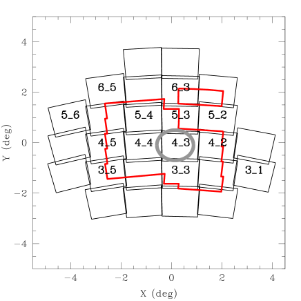
Figure 1: Celestial distribution of OGLE III footprint (red contours) and VMC tiles (black rectangles) in the SMC area. $X$ and $Y$ are defined as in van der Marel & Cioni (2001) with $\alpha_{0}=12.5$ deg and $\delta_{0}=-73.0$ deg. Tiles analysed in this work are labelled with their VMC IDs. The grey oval shows the area containing the peak density of the SMC CCs which was avoided in the present analysis.

The SMC tiles analysed in this work are the ones for which the VMC observations were completed before 2014 September 30. They are tiles SMC 3_3, 3_5, 4_2, 4_3, 4_4, 4_5, 5_2, 5_3, 5_4, 6_3 and 6_5, labelled with their IDs in Fig. 1. The lower portion of Table 1 lists centre coordinates and observation properties for all of them. OGLE III observations cover the most central and crowded regions of the SMC. In particular, the peak in stellar density (see Figure 1 of Rubele et al. 2015) and CC density (see right panel of Figure 18 in Moretti et al. 2014) in the SMC occurs in an area centered at coordinates RA=12 deg, Dec=$-$73.1 deg and radius of 2 deg in RA and 0.5 deg in Dec. This region, marked by a grey oval in Fig. 1, mainly covers the tile SMC 4_3 and contains 1695 of the 4630 CCs identified by the OGLE III survey in the SMC. However, as we aim at fine-tuning our procedures to identify new SMC CCs outside the OGLE III field (see Section 4), we considered in the following analysis only CCs lying in the external portions of the OGLE III footprint, where the level of crowding and reddening is similar to what we found in the regions which currently have only VMC data (see Fig. 1). Specifically, we considered 2935 CCs located outside the oval shape in Fig. 1. By matching the OGLE III and VMC catalogues, using a pairing radius of 0.5 arcsec we obtained a sample of 2411 CCs that have VMC $K_{\mathrm{s}}$-band light curves. Increasing the paring radius to 1.0 arcsec would result in increasing by about 1% the number of misidentifications. Conversely, reducing the paring radius to 0.1 arcsec, would result in loosing about 10% of the crossmatched sources. On the other hand, the reliability of our cross-identifications and, in turn, of the value adopted for the paring radius, is specifically assessed by folding the VMC $K_{\mathrm{s}}$-band light curves according to the corresponding OGLE III periods (e.g. Ripepi et al. 2015). These CCs lie in the tiles (see Fig. 1): SMC 3_3, 3_5, 4_2, 4_3 and 4_4 (excluding sources inside the oval grey contour), 4_5, 5_2 (two sources), 5_3, 5_4, 6_3 (four sources) and 6_5 (two sources).

3.1 Selection based on the colour-magnitude and colour-colour diagrams

We used the sample of 2411 OGLE III CCs described in the previous section as a reference to define the range in VMC colours and magnitudes in which the SMC CCs lie. Figure 2 shows the distribution of such stars in the ($J-K_{\mathrm{s}}$, $K_{\mathrm{s}}$) colour-magnitude diagram. We have highlighted with red dashed contours the region that we will use to select CC candidates. We note that 2365 of the 2411 reference CCs (corresponding to 98% of the sample) have $\langle K_{\mathrm{s}}\rangle<$ 17.0 mag and only 2% of the population have fainter magnitudes. Specifically, 45 stars have $17.0\leq\langle K_{\mathrm{s}}\rangle\leq$ 18.2 mag and only 1 CC is as faint as $\langle K_{\mathrm{s}}\rangle$ = 18.6 mag. We have also reported in Fig. 2 the theoretical instability strips (ISs) for CCs with metallicity Z=0.004 and helium abundance $Y$=0.25 taken from Bono et al. (2000, 2001a, 2001b). These values of $Z$ and $Y$ are appropriate for the SMC CCs. To transform the theoretical IS edges to the observational plane we adopted the static model atmospheres by Castelli et al. (1997a, b), an absorption $A_{V}$=0.1 mag (Haschke et al., 2011) and a distance modulus of 19.0 mag, computed as the weighted average of the CC results in table 1 of Haschke et al. (2012).

Specifically, we have plotted in Fig. 2 the blue and red edges of the IS for CCs of different pulsation modes: F (grey lines), 1O (green lines) and 2O (magenta lines). For magnitudes brighter than 14 mag, there is reasonably good agreement, within the errors, between theoretical and observed IS’s, suggesting that the sample of CCs we are using as reference (Soszyński et al., 2010a), once matched with the VMC data, represents the ranges in $K_{\mathrm{s}}$ magnitude and $J$-$K_{\mathrm{s}}$ colour covered by the SMC CCs very well. A number of reference CCs, especially at magnitudes fainter than $K_{\mathrm{s}}\sim$14 mag, are found beyond the boundaries of the theoretical IS’s, both at bluer and redder colours. This is likely caused by metallicity, differential reddening issues and by the poor sampling of their VMC $J$-band light curves. Indeed, the same theoretical ISs are in much better agreement with other observational samples, including Magellanic Cepheids, where light curves are better sampled in colour (e.g. Bono et al. 1999, Marconi et al. 2005). We also compared the colour-magnitude distribution for sources with more than 10 data points in the $J$ band (about 10% of our sample) using the $J$-$K_{\mathrm{s}}$ colours obtained after analyzing both the $J$ and $K_{\mathrm{s}}$-band light curves with a custom template fitting procedure (Ripepi et al., 2015, 2016). We obtained a relatively more compact distribution, confirming that the poor sampling of the VMC $J$-band light curves is one of the possible issues.

The right panel of Figure 2 shows the distribution of these CCs in the $Y-J$, $Y-K_{\mathrm{s}}$ colour-colour diagram. As in Fig. 2, we have highlighted with red dashed contours the region that we will use in Sec. 4 to select CC candidates.

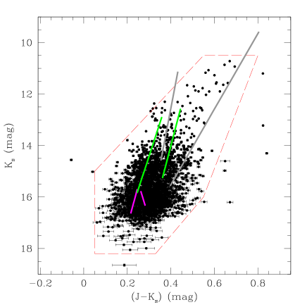
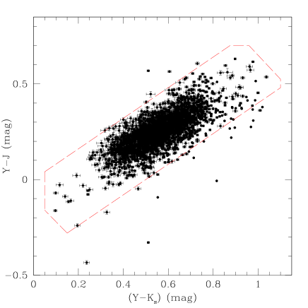
Figure 2: Left: Distribution of known SMC CCs in the ($J-K_{\mathrm{s}}$, $K_{\mathrm{s}}$) colour-magnitude diagram. Grey, green and magenta solid lines represent the theoretical blue and red edges of the CC ISs for F, 1O and 2O pulsation modes, respectively. Right: Same as the left panel but in the ($Y-J$, $Y-K_{\mathrm{s}}$) colour-colour diagram. In both panels, red dashed contours indicate the boundaries of the region that will be used to select candidate CCs in the external part of the SMC. See Section 3 for details.

3.2 Analysis of the light curves

OGLE III periods of the reference CCs range between 0.25 d to 208 d. The vast majority of the reference CCs (2240 sources) have $P$$<$5d, 109 sources have $5\leq$$P$$<$10 d, 60 have $10\leq$$P$$<$75 d and only 2 sources have $P$$\geq$75 d. Specifically, these two sources have $P_{\rm OGLE}$= 128.2 d and $P_{\rm OGLE}$ =208.8 d; despite their $K_{\mathrm{s}}$-band photometry ($K_{\mathrm{s}}\sim$ 11 mag) should not be saturated, they are fainter than expected according to the $K_{\mathrm{s}}$-band $PL$ relation, especially the last one. The same feature occurs in the $I$-band OGLE data. Despite their images do not show any clear problem, their folded $K_{\mathrm{s}}$-band light curves are very noisy without a clear shape; for these reasons we decided to discard them and focus on the sources with $P$ lower than 80 d.

We analysed the $K_{\mathrm{s}}$-band light curves and derived the period of the reference CCs from the $K_{\mathrm{s}}$ time-series data alone, ignoring OGLE III information on the period. We used all available VMC epochs to study the light curves including observations obtained during nights with sky conditions (i.e. seeing and ellipticity) that exceeded the VMC requirements (Cioni et al., 2011), since our fitting procedure is able to handle lower accuracy data (see, e.g., Ripepi et al. 2015 and references therein). The resulting light curves have a number of data points that ranges from 7 to 60. We checked the images of some CCs with a few epochs and found that often these sources are contaminated by very bright companions.

Periods were derived using the program “Significance Spectrum” (SigSpec; Reegen 2011). SigSpec is a method specifically developed for detecting and characterizing periodic signals in noisy data. While most period search analyses explore only the Fourier amplitude, through the power spectrum, ignoring phase information, SigSpec is based on the definition of a quantity called spectral significance for a time series, a function of Fourier phase and amplitude. The spectral significance quantity conveys more information than does the conventional amplitude spectrum alone, and appears to simplify statistical issues as well as the interpretation of phase information.

We ran SigSpec on the VMC $K_{\mathrm{s}}$-band time-series adopting a lower period of 0.25 d, an upper period of 80 d and weighting by the $K_{\mathrm{s}}$ single-epoch errors. The r.m.s. of the light curve analysis typically ranged from 0.002 mag to 0.15 mag, (with a few extreme values as large as 0.3 mag) and a median value of 0.015 mag. The median value of the spectral significance is $\sim$ 3.0 with a standard deviation of 0.9, and minimum and maximum values of 0.9 and 7.0 (see also discussion at the end of Section 3.3). Figure 3 shows the comparison between the OGLE III periods and the periods we derived for the reference CCs running SigSpec on the $K_{\mathrm{s}}$ time-series data. For 54% of the sources (1302 stars) the two periods are in good agreement, the difference being smaller than 0.02 d. On the other hand, for some stars the period found by SigSpec ($P_{\rm SigSpec}$) is definitely shorter than that published by the OGLE team. In particular, about 800 sources have $\Delta P$=$P_{\rm OGLE}$ (where $\Delta P$=$P_{\rm OGLE}-P_{\rm SigSpec}$) because their $P_{\rm SigSpec}$ is near zero (see Fig 3). This is probably due to alias problems in the case of sources with period shorter than a few days and to saturation of the $K_{\mathrm{s}}$ time series for stars with longer period. Conversely, there are about 150 stars for which $P_{\rm SigSpec}$ is definitely longer than $P_{\rm OGLE}$ and hence $\Delta P$ assumes large negative values (see Fig 3). This might be due to faintness and hence poor quality of the $K_{\mathrm{s}}$ light curves of these stars that affect the period search procedure. We also checked if there is any dependence of $\Delta P$ on the amplitude of the light curves, but did not find any. We do not have an estimate of the error on $P_{\rm SigSpec}$ for each star but, assuming the OGLE as the correct one, we can use as an estimate of the $P_{\rm SigSpec}$ error the median value of $\Delta P$, that is 0.002 d.

As an additional test, we performed an analysis of the $K_{\mathrm{s}}$ light curves using a different period search program, FNPEAKS (Kurtz, 1985). We adopted the same limits (0.25-80 d) for the period and a frequency step of 0.0001 s^-1. For 29% of the stars there is good agreement between the OGLE IIII and the FNPEAKS periods: $\arrowvert\Delta$P$\arrowvert\leq$ 0.02 d. FNPEAKS does not allow to weight by the error of the single epoch magnitudes; this probably explains the lower percentage of periods recovered within 0.02 d with respect to SigSpec (54%). We also checked the $P$ versus $\Delta P$ plot, that is the counterpart of Fig. 3. The shape of the $\Delta P$=$P_{\rm OGLE}-$$P_{\rm FNPEAKS}$ versus $P_{\rm OGLE}$ is very similar to Fig. 3, hence confirming that FNPEAKS and SigSpec find consistent results, however, SigSpec appears to be more efficient. In the analysis described in Sec. 4 we will thus adopt SigSpec to estimate the period of the candidate variable stars.

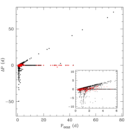
Figure 3: Distribution of $\Delta P$=$P_{\rm OGLE}-P_{\rm SigSpec}$ versus $P_{\rm OGLE}$. Shown in the inset is an enlargement of the short period region. Red points indicate stars within 3 $\sigma$ from the $PL$ relations but with $\Delta P$ larger than 0.02 d. See text and Fig. 4 for details.

3.3 Selection based on the Period-luminosity relation

Figure 4 shows the $K_{\mathrm{s}}$-band period-luminosity ($PL$) plane obtained for the 2411 reference CCs using for the period values derived with the SigSpec analysis and for the $K_{\mathrm{s}}$ average magnitude values available from the VSA. Red solid lines show the $PL$ fits obtained for F and 1O mode CCs, using the periods from OGLE III; red dashed lines show the corresponding 3$\sigma$ boundaries for 1O (upper dashed line) and F (lower dashed line) CCs, respectively. As expected, Cepheids with a good SigSpec estimate of the period ($\arrowvert\Delta$P$\arrowvert\leq$0.02 d, black points) lie near the $PL$s defined using the OGLE III periods. Specifically, there are 1589 objects lying within 3$\sigma$ from the $PL$s, corresponding to 66% of the original sample. This number includes 1304 stars with $\arrowvert\Delta$P$\arrowvert\leq$ 0.02 d (black points) and 285 sources with $\arrowvert\Delta$P$\arrowvert$ larger than 0.02 d (grey points). These 285 sources are marked by red points in the $\Delta$P versus $P_{\rm OGLE}$ distribution shown in Fig. 3. The bulk of the distribution has $\arrowvert\Delta$P$\arrowvert\leq$ 1 d (253 objects), and only a few sources (32 stars) have $\Delta$P values larger than $\pm$ 1 d and up to 2.5 d.

Stars within the 3$\sigma$ from the $PL$s, show an average significance (see Section 3.2) of 3.4 with minimum and maximum values of 1.8 and 7.0, respectively. We checked the position of these stars on the $PL$ according to their $significance$ value and noted that several stars with significance value between 1.8 and 2.0 lie within 2$\sigma$ from the $PL$s. Hence, in the following analysis we will retain only sources with significance larger than 1.7 (Section 4). We will also take into account the possible contamination by other types of variable stars. In particular, the RR Lyrae stars follow a $PL_{K_{\mathrm{s}}}$ relation that, although different, partially overlaps with the $PL_{K_{\mathrm{s}}}$ relation of CCs. A black dashed box schematically shows the locus of the SMC RR Lyrae stars in the $K_{\mathrm{s}}$-band $PL$ plane in Fig. 4. This issue will be discussed in more detail in Section 4.1.

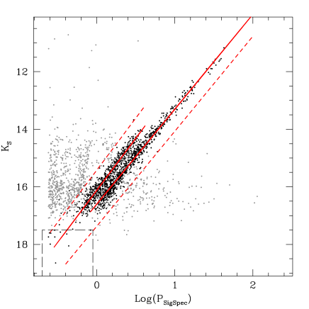
Figure 4: Distribution of known SMC CCs in the Period-$K_{\mathrm{s}}$-band Luminosity plane using for the period values derived from the analysis of the $K_{\mathrm{s}}$-band light curves. Red solid lines show the $PL$ relations for F (right) and 1O (left) CCs derived using the OGLE III periods. Red dashed lines represent 3$\sigma$ boundaries of the 1O (upper line) and F (lower line) $PL$s, respectively. Black and grey dots show stars with $\arrowvert\Delta$P$\arrowvert\leq$0.02 d and $\arrowvert\Delta$P$\arrowvert>$ 0.02 d, respectively. A black dashed box marks the region populated by RR Lyrae stars. See Section 4.1 for details.

3.4 VSA flags

The VSA provides several flags describing the quality of the light curve of each VMC source. A complete explanation of these parameters is provided in Cross et al. (2012) and on the VSA web page. Here we briefly summarize the properties that are relevant for the present study. The VSA classifies sources according to their nature by the $mergedClass$ parameter within the $vmcSource$ table, containing the information about the sources extracted from the stacked images. Specifically, the association between parameter value and physical nature of the source is as follows: 1=galaxy, 0=noise, $-1$=stellar, $-2$=probableStar, $-3$=probableGalaxy, $-9$=saturated source. The $KsppErrBits$ parameter encodes quality issues associated with a given $K_{\mathrm{s}}$-band detection within the vmcSource table. Its value is zero for a detection without quality issues and grows according to the severity of the issue. In particular to include sources with only minor $K_{\mathrm{s}}$-band quality issues the user can filter as $KsppErrBits<$256.

We used the VSA flags to select among our sample of 2411 reference CCs only stars with at least 10 data points (this corresponds to 2407 of the 2411 sources), that are classified as stars or probable stars by the VSA ($mergedClass$=$-$1 or $-$2), as variables ($VarClass$=1) and that do not exibit any severe quality issues ($KsppErrBits<$256), thus ending up with a total of 1445 sources. This corresponds to 60% of our original sample. Five hundred of the sources that the VSA classifies as non variable sources ($VarClass$=0) perfectly lie within the 3$\sigma$ limits from the $PL$s. Hence, the VSA flags, although useful for a first selection of variable sources, need to be fine-tuned (see, e.g., Ferreira Lopes & Cross 2015) to increase their capability to detect bona fide variable stars. In the next section we will use the VSA flags to corroborate our identification of new SMC CCs based on the colour-magnitude and colour-colour diagrams and $PL$ selections described in the previous sections.

In conclusion, to identify CCs from the VMC $K_{\mathrm{s}}$-band time series data we will

• first select candidate variables by applying the colour-magnitude and colour-colour diagrams cuts described in Section 3.1,

• analyse with SigSpec the light curves of the candidate variables to determine their periods (see Section 3.2),

• consider as best candidates the stars falling within 3$\sigma$ from the $PL$s defined as described in Sec. 3.3,

• investigate the VSA flags.

In this way, following a visual inspection of the light-curves to identify bona fide CCs, we should be able to identify 66% of the CCs that populate the external areas of the SMC analysed in the next Section.

4 Detection of classical Cepheids in the external regions of the SMC

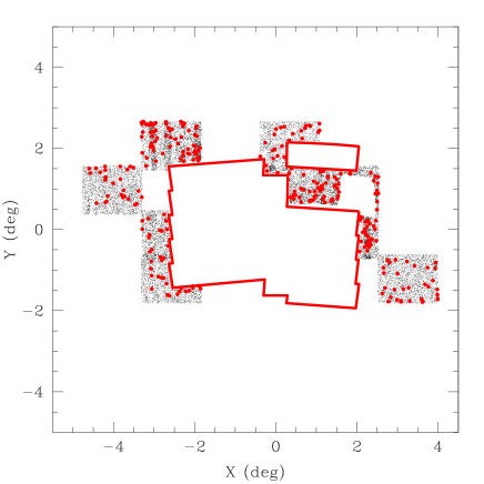
Figure 5: Spatial distribution of the SMC CC candidates (black points) selected using the tools described in Section 3. $X$ and $Y$, the red contours and the VMC tiles are defined as in Fig. 1. The white area within tile SMC 5_2 at $X\sim 2$, $Y\sim 1$ corresponds to the 47 Tucanae field analyzed by Weldrake et al. (2004). Sources that we confirm to be bona fide new Cepheids are marked by red filled circles (see text for details).

We have applied the methods described in Section 3 to look for CCs in all regions of the SMC where we currently have complete VMC data, but where no optical comprehensive catalogue of variable stars is available yet. Figure 5 shows the portion of sky we have analysed with the different VMC tiles labelled in Fig. 1 (see also Tab. 1). We specifically considered only regions outside the OGLE III footprint (red solid lines) and also discarded the region studied by Weldrake et al. (2004; empty area within tile SMC 5_2 at $X\sim 2$, $Y\sim 1$), who provided a comprehensive catalogue of variable stars in the field of the Galactic globular cluster 47 Tucanae. In particular, we first selected our candidates in the aforementioned VMC tiles, and then discarded sources lying in the region that overlaps with the OGLE III and Weldrake et al. (2004) fields. The sources were then further selected using the colour-magnitude and colour-colour diagrams, as described in Section 3.1, yielding 19,938 candidate CCs, that are plotted as black points in Fig. 5.

Rubele et al. (2015) estimated the star formation history (SFH) in these regions of the SMC. By comparing the best-fitting SFH models with the theoretical CC instability strips for $Z$=0.004 and $Y$=0.25 we predict a few hundreds CCs to populate the area under investigation. Hence, clearly, only a few percent of our 19,938 CC candidates are bona fide CCs. For 18,090 of these sources the VSA provides $K_{\mathrm{s}}$-band light curves with at least 10 data points, we analysed them with SigSpec and defined their period following the procedure described in Section 3.2. Furthermore, we derived average $K_{\mathrm{s}}$ magnitudes and $K_{\mathrm{s}}$-band amplitudes (Amp$K_{\mathrm{s}}$) analysing the light curves with an automatic template fitting procedure specifically developed for the analysis of the $K_{\mathrm{s}}$-band light curves of the SMC CCs (Ripepi et al., 2016). We then used the periods derived with SigSpec and the average $K_{\mathrm{s}}$ magnitudes computed as described above to plot the sources in the Period - $K_{\mathrm{s}}$ Luminosity plane shown in Fig. 6. We have also plotted in this figure the 3$\sigma$ boundaries of the $K_{\mathrm{s}}$-band $PL$ relations defined by the OGLE III SMC CCs (see Section 3.3).

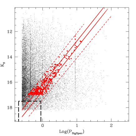
Figure 6: Distribution of the 18,090 candidate CCs (black points) in the Period - $K_{\mathrm{s}}$-band Luminosity plane. Red solid lines show the $PL$ relations and their 3$\sigma$ boundaries (red dashed lines) defined by the OGLE III SMC CCs. A black dashed box highlights the region occupied by the SMC RR Lyrae stars. Red filled circles mark bona fide CCs identified in the present study. Their $K_{\mathrm{s}}$-band light curves are shown in Fig. 7.

Excluding objects more than 3$\sigma$ away from the F and 1O mode $PL$ relations the sample reduces to 4,817 sources.

We further selected the sample using the parameters of the template fitting procedure. A comprehensive description of this procedure and of its parameters is provided by Ripepi et al. (2016). Here we simply note that we used the parameter $G$, which gives an estimate of the goodness of the fit by weighting the residuals of the fit (rms) with the number of data points rejected (outliers) from the fitting procedure. The first term of $G$ tends to favour templates which give the smallest rms values, whereas the second term favours those removing the least number of outliers. The balance between these two terms generally yields an automatic selection of the best templates that is in agreement with the visual inspection of the fitting procedure. Since $G$ is inversely proportional to the square of the rms and directly proportional to the fourth power of the ratio between used in the fit and total number of phase points in the light curve, values of $G$ in the interval 100-10000 generally mean good fit, and, in absolute terms, also good light curve with small scatter. On the contrary, values of $G$ below 100 are usually associated with highly scattered light curves. Finally, we retained only sources with the $G$ parameter between 100 and 10,000 and $K_{\mathrm{s}}$-band amplitude $\geq$ 0.04 mag further reducing the sample to 3,636 best candidates with $\langle K_{\mathrm{s}}\rangle$ magnitude in the range of 12.31 to 18.21 mag. This number appears to be still rather large if compared to expectations from the SFH recovery. A check was made by comparing the distributions of CCs in the VMC tiles partially covered by OGLE III. In particular, half of the tile SMC 4_5 is covered by both OGLE III and VMC and the other half only by VMC (see Figs. 1 and 5). We divided the tile into four subregions, each of them approximately covering the same area. The two western subregions lie within the OGLE III footprint, while the two eastern ones lie outside. OGLE III detected 53 CCs in the north-western subregion and 30 in the southern one. From the SFH performed by Rubele et al. (2015) and the theoretical IS’s (Bono et al. 2000, 2001a, 2001b), we obtain a total number of about 55 (with a minimum of 35 and a maximum of 76) CCs from the SFH recovery, in good agreement with the OGLE III findings. Our number of CC candidates in the two eastern subregions of tile SMC 4_5 is roughly 10 times that observed by OGLE III in the two western ones. This test suggests that the majority of the 3636 new candidate variable stars are not CCs and that a high level of contamination must be present among them. In particular there could be contamination by other types of variables, but also issues such as: saturation (on the bright side), limiting magnitude and photometric error problems (on the faint side), blending effects, intrinsic problems of the NIR data, etc. These issues may particularly affect faint sources, thus leading to an overestimate of the number of variable sources. Indeed, the sample of 3,636 new candidate variables includes 1,677 sources with $\langle K_{\mathrm{s}}\rangle<$ 17.0 mag and 1,959 fainter sources with $17.0\leq\langle K_{\mathrm{s}}\rangle\leq$ 18.2 mag. However, according to the discussion in Section 3.1, only 2% of the SMC CCs have $\langle K_{\mathrm{s}}\rangle$ magnitudes fainter than 17.0 mag. Hence, the 1,959 candidate variables fainter than 17.0 mag should include, at most, $\sim$ 40 bona fide CCs. We hence visually inspected only the $K_{\mathrm{s}}$ light curves of all 1,677 sources brighter than $\langle K_{\mathrm{s}}\rangle$= 17.0 mag and selected among them 297 sources whose $K_{\mathrm{s}}$-band light curves have the typical shapes of CCs. In particular, all sources with very poor light curve coverage were discarded since a firm classification was not possible. Moreover, for several sources the light curves did not show the typical shape of cepheids, these sources were discarded as well. During the visual inspection, a percentage reliability flag has been assigned to each source. This flag is 100% for a source with (i) good phase coverage, (ii) good light curve shape and (iii) good position in the PL, while its value diminishes according to issues related to one or more of the aforementioned features, becoming 62% for sources that are not confirmed to vary.

Then we also checked a subsample of 240 among the 1,959 sources fainter than $\langle K_{\mathrm{s}}\rangle$ = 17.0 mag; this provided two additional sources with light curves typical of CCs. Particular attention was devoted to sources showing a $K_{\mathrm{s}}$-band amplitude between 0.04 mag and 0.1 mag since at this level of amplitude it is hard to distinguish between real variable sources and spurious objects. We hence decided to keep only low amplitude sources with a good light curve coverage and very clear shapes.

We consider this total sample of 299 candidate variable stars that passed the colour-magnitude and colour-colour diagrams, $PL$, template parameters selections and the visual inspection of the light curve as bona fide Cepheids. Out of 299, nine sources are in common with the General Catalog of Variable Stars (GCVS, Artyukhina et al. 1996), two (VMC-SMC-CEP-258 and 286) are ACs in common with Soszyński et al. 2015a, while 288 are new CCs identified in the present study. The new CCs have periods in the range from about 0.34 to 9.1 d and span the magnitude range: 12.9 $\leq\langle K_{\mathrm{s}}\rangle\leq$ 17.6 mag, and only two being fainter than 17.0 mag (see above). This number is well consistent with the predictions of Rubele et al. (2015) SFH recovery in these external regions of the SMC. In particular, of the 299 confirmed Cepheids, only 13 are located in the eastern subregions of tile SMC 4_5. In the same two subregions Rubele et al. (2015) SFH recovery leads to a total number of about 10 (with a minimum of 4 and a maximum of 20) CCs, in very good agreement with our findings.

Table 3 lists our 299 SMC Cepheids along with their RA, Dec (J2000) coordinates, the period obtained with SigSpec (for a discussion about the errors see Section 3.2), the $K_{\mathrm{s}}$-band amplitude and the intensity-averaged $K_{\mathrm{s}}$ magnitude computed with the template-fitting procedure, the VarClass parameter attributed by the VSA and the variability type (VarType) assigned in the present study together with comments, if any, and the aforementioned percentage reliability flag. The last column of Table 3 also provides the GCVS identification number, whenever appropriate. The sources are ordered by increasing magnitude going from brighter to fainter objects. Their spatial distribution over the SMC is shown in Fig. 5 where they have been marked as red filled circles.

Table 3: Information on the 299 Cepheids that we have identified in the SMC using only the near-infrared photometry of the VMC survey. Col. 1: VMC-SMC-CEP ID, Col. 2: Right Ascension (RA, J2000), Col. 3: Declination (Dec, J2000), Col. 4: number of $K_{\mathrm{s}}$ observations, Col. 5: period computed with SigSpec, Col. 6: $K_{\mathrm{s}}$ amplitude computed with the template fitting procedure, Col. 7: intensity-averaged $K_{\mathrm{s}}$ magnitude computed with the template fitting procedure, Col. 8: VarClass flag assigned by the VSA, Col. 9: variability type assigned in the present study, corresponding percentage reliability flag and specific comments, if any. The table is published in its entirety as Supporting Information with the electronic version of the article. A portion is shown here for guidance regarding its form and content.

VMC ID	RA	Dec	$N_{K_{\mathrm{s}}}$	$P_{\rm SigSpec}$	Amp$K_{\mathrm{s}}$	$\langle K_{\mathrm{s}}\rangle$	VarClass	VarType & Comments
	(deg)	(deg)		(d)	(mag)	(mag)
001	01:43:58.77	$-$71:50:09.7	18	8.89656	0.06	12.350	0	75% CC few points at min
002	01:43:15.53	$-$71:42:49.8	18	8.897351	0.08	12.599	0	75% CC few points at min
003	01:28:07.58	$-$72:48:52.1	18	12.52367	0.27	12.758	1	100% CC GCVS2347
004	01:24:25.35	$-$74:16:50.5	16	13.151942	0.29	12.792	1	100% CC GCVS2343
005	01:42:56.52	$-$71:18:46.0	18	9.122673	0.05	12.885	0	75% CC few points at min
006	01:38:18.83	$-$71:22:18.4	18	8.886835	0.04	13.076	0	75% CC few points at min
007	01:23:00.57	$-$74:22:16.8	16	9.752387	0.21	13.182	1	100% CC GCVS2337
008	01:38:00.64	$-$71:39:22.2	18	8.887862	0.06	13.269	0	75% CC few points at min
009	00:29:43.53	$-$71:33:21.0	17	8.371283	0.06	13.470	0	100% CC
010	01:13:25.40	$-$70:58:09.2	14	5.233301	0.06	13.533	0	75% CC few points at min

During the revision phase of this manuscript, Soszyński et al. (2015b) paper presenting CCs in the Magellanic Clouds was posted as a preprint on the ArXiv. The authors comment that they can counter-identify 278 sources out of the 299 Cepheids in our list (the remaining 21 fall in the inter-CCD gaps of their camera; Soszynski, private communication) and they confirm 35 of the SMC Cepheids we have identified in our study. They also say that most of the remaining objects from our list turned out to be constant or nearly constant in the optical bands. We have cross-matched our catalogue with Soszyński et al. (2015b)’s and find that indeed 36 (about 13%) of our Cepheids are confirmed by OGLE IV, namely, the nine CCs in common with the GCVS, the two ACs also identified by Soszyński et al. (2015a) and 25 new CCs. This result is encouraging, since it confirms that our method is promising despite the limited number of data points and the intrinsically low amplitude of the VMC light curves. But it is also quite puzzling due to the low rate of optical confirmations, since our 299 bona fide Cepheids were selected not simply because of the light variation in the $K_{\mathrm{s}}$-band, but, more importantly, because they also fall in the colour-magnitude and colour-colour diagrams where OGLE III SMC bona-fide Cepheids are found, and because they also follow the SMC Cepheid $PL$ relation.

The $K_{\mathrm{s}}$-band light curves of our 299 bona fide SMC Cepheids folded according to the period derived from the analysis with SigSpec, are shown in Fig. 7. We first display the 9 CCs in common with the GCVS and the 25 new CCs discovered in our study and later confirmed also by OGLE IV; all other bona fide Cepheids (including the two ACs) follow. The light curves appear overall quite symmetrical and it is difficult with the VMC $K_{\mathrm{s}}$-band data to identify features such as bumps. $K_{\mathrm{s}}$ time series data for all of them are provided in Table 4. Among the remarks in the last column of Tab. 3, “few points at min/max” is used whenever the light curve is not homogeneously covered at minimum or maximum light. For some of these sources, we checked the light curve of nearby sources within 5 arcsec, to rule out unidentified photometric problems that might cause/mimic the light variation. They look flat suggesting that the variability of the sources identified as Cepheids is real, even for less well sampled light curves.

Finally, we recall that according to the results in Section 3.3 our technique enables recovery of about a 66% of the true Cepheids that may occur in these external regions of the SMC and that bona fide Cepheids may also be present in the sample of about 2,000 candidate variables fainter than $K_{\mathrm{s}}$ = 17.0 mag that were not analyzed here. Therefore, there are likely additional Cepheids that we may have missed either because their SigSpec periods are wrong by more than $\pm$ 2.5 d, thus causing them to fall outside the 3$\sigma$ boundaries of the $PL$s, or because they are fainter than $K_{\mathrm{s}}$ = 17.0 mag.

Table 4: $K_{\mathrm{s}}$-band time-series photometry of our 299 SMC Cepheids. The table is published in its entirety as Supporting Information with the electronic version of the article. A portion is shown here for guidance regarding its form and content.

Star VMC-SMC-CEP-001
HJD-2400000	$K_{\mathrm{s}}$	err$K_{\mathrm{s}}$
(d)	(mag)	(mag)
55834.792559	12.339	0.002
55927.600518	12.344	0.002
56146.865651	12.336	0.002
56147.757493	12.336	0.002
56155.743101	12.336	0.002
56159.787169	12.342	0.002
56163.761878	12.327	0.002
56175.694234	12.330	0.002
56188.672502	12.389	0.002
56189.703199	12.360	0.002
56190.724434	12.334	0.002
56208.619677	12.337	0.002
56226.551935	12.335	0.002
56256.553723	12.336	0.002
56282.578397	12.333	0.002
56300.546758	12.329	0.002
56486.866850	12.326	0.002
56911.795036	12.331	0.002

Figure 7: $K_{\mathrm{s}}$-band light curves of bona fide Cepheids in the external regions of the SMC identified in the present study. For each source we indicate the VMC ID (ordered by increasing magnitude; see also Tab. 3) and the period derived from the analysis of the light curve with SigSpec. We first display the 9 CCs in common with the GCVS (VMC-SMC-CEP-003, 004, 007, 011, 022, 039, 041, 051, 091) and 25 new CCs discovered in our study that were later confirmed also by OGLE IV (VMC-SMC-CEP-023, 035, 038, 042, 056, 075, 081, 085, 087, 093, 097, 101, 110, 121, 133, 136, 138, 140, 161, 166, 177, 188, 231, 237, 292). All other bona fide Cepheids (including the two ACs) follow. The figure is published in its entirety as Supporting Information with the electronic version of the article.

4.1 Contamination by other types of variable stars

Adopting as reference the catalogue of RR Lyrae stars detected in the SMC by the OGLE III survey (Soszyński et al., 2010b), Muraveva et al. (in prep.) studied the $K_{\mathrm{s}}$-band $PL$ relation of 1,081 SMC RR Lyrae stars observed by VMC. They found that these variables typically have $K_{\mathrm{s}}$ mean magnitude between 17.5 mag and 19.5 mag, with a subset of about 200 of them having 17.5 $\leq\langle K_{\mathrm{s}}\rangle\leq$ 18.2 mag. In this magnitude range there is partial overlap with the short period, faint end of the CCs distribution (see Fig. 2). Furthermore, while the number of CCs is expected to drop significantly moving from the centre to the external region of the SMC, the distribution of RR Lyrae stars declines gently and their number is expected to remain rather high in the peripheral areas we are investigating (e.g. Fig. 7 of Soszyński et al. 2015a). Therefore, some of the 1,959 candidate variables with $17.0\leq\langle K_{\mathrm{s}}\rangle\leq$ 18.2 mag may be RR Lyrae stars.

A further three percent contamination can also be expected from ECLs, they can spread all over the colour-magnitude diagram (see Moretti et al. 2014), thus we would need different criteria to distinguish them.

Finally, some of the sources could be ACs like VMC-SMC-CEP-258 and 286, or T2Ceps, due to the partial overlap existing among the $PL$s of the different types of Cepheids, especially between CCs and ACs (e.g. Soszyński et al. 2008b).

5 Summary and conclusions

We have developed a technique to identify variable stars using only the multi-epoch near-infrared photometry obtained by the VMC survey and have specifically tailored it to the identification of Cepheids. The technique exploits colour-magnitude and colour-colour diagrams, and $PL$ relations defined by known SMC Cepheids, along with template parameter selections and visual inspection of the light curve to identify bona fide Cepheids. The technique was applied to external regions of the SMC for which complete VMC $K_{\mathrm{s}}$-band observations are available and no comprehensive identification of variable stars from other surveys exists yet. We have identified and present $K_{\mathrm{s}}$-band light curves for 299 SMC Cepheids, of which 9 are CCs in common with the General Catalog of Variable Stars (GCVS, Artyukhina et al. 1996), two are ACs also found by Soszyński et al. (2015a) and the remaining 288 sources are new discoveries. The number of SMC Cepheids we have detected is consistent with the predictions of Rubele et al. (2015) SFH recovery in these regions of the SMC, taking into account that our technique may enable recovery of only about a 66% of the true Cepheids that may occur in these external regions of the SMC. Subsequently, Soszyński et al. (2015b) crossmatched 278 of the sources in our list with their optical photometry and confirmed 36 of them as Cepheids. This result is encouraging, since it shows that our technique is promising despite the limited number of data points and the intrinsically low amplitude of the VMC light curves, but the low rate of optical confirmations is rather surprising and calls for further investigations to understand this discrepancy and possible physical/technical reasons behind it. This near-infrared vs optical light-curve connection/conspiracy will be addressed in a following paper.

References

- Alcock et al. (2000) Alcock C., et al. 2000, ApJ , 542, 281
- Artyukhina et al. (1996) Artyukhina, N. M., Durlevich, O. V., Frolov, M. S., et al. 1996, VizieR Online Data Catalog, 2205,
- Bailey (1902) Bailey, S. I. 1902, Annals of Harvard College Observatory, 38, 1
- Bono et al. (2001a) Bono, G., Caputo, F., & Marconi, M. 2001, MNRAS , 325, 1353
- Bono et al. (1999) Bono, G., Caputo, F., Castellani, V., & Marconi, M. 1999, ApJ , 512, 711
- Bono et al. (2000) Bono, G., Castellani, V., & Marconi, M. 2000, ApJ , 529, 293
- Bono et al. (2001b) Bono, G., Gieren, W. P., Marconi, M., & Fouqué, P. 2001, ApJ , 552, L141
- Caputo et al. (2000) Caputo, F., Marconi, M., & Musella, I. 2000, A&A , 354, 610
- Castelli et al. (1997a) Castelli, F., Gratton, R. G., & Kurucz, R. L. 1997a, A&A , 318, 841
- Castelli et al. (1997b) Castelli, F., Gratton, R. G., & Kurucz, R. L. 1997b, A&A , 324, 432
- Cioni et al. (2011) Cioni M.-R. L., Clementini G., Girardi L., et al. 2011, A&A , 527, A116
- Cioni et al. (2013) Cioni, M.-R. L., Anders, P., Bagheri, G., et al. 2013, The Messenger, 154, 23
- Cross et al. (2009) Cross, N. J. G., Collins, R. S., Hambly, N. C., et al. 2009, MNRAS , 399, 1730
- Cross et al. (2012) Cross N. J. G., Collins R. S., Mann R. G., et al. 2012, A&A , 548, A119
- de Grijs & Bono (2015) de Grijs, R., & Bono, G. 2015, AJ , 149, 179
- Emerson et al. (2006) Emerson, J., McPherson, A., & Sutherland, W. 2006, The Messenger, 126, 41
- Ferreira Lopes & Cross (2015) Ferreira Lopes C. E., Cross N. J. G.,2015 arXiv:1506.04914
- Graczyk et al. (2011) Graczyk, D., Soszyński, I., Poleski, R., et al. 2011, Acta Astron. , 61, 103
- Haschke et al. (2011) Haschke, R., Grebel, E. K., & Duffau, S. 2011, AJ , 141, 158
- Haschke et al. (2012) Haschke, R., Grebel, E. K., & Duffau, S. 2012, AJ , 144, 107
- Kozłowski et al. (2013) Kozłowski, S., Udalski, A., Wyrzykowski, Ł., et al. 2013, Acta Astron. , 63, 1
- Kurtz (1985) Kurtz, D. W. 1985, MNRAS , 213, 773
- Lewis et al. (2010) Lewis, J. R., Irwin, M., & Bunclark, P. 2010, Astronomical Data Analysis Software and Systems XIX, 434, 91
- Liu & Janes (1990) Liu, T., & Janes, K. A. 1990, ApJ , 354, 273
- Marconi et al. (2005) Marconi, M., Musella, I., & Fiorentino, G. 2005, ApJ , 632, 590
- Moretti et al. (2014) Moretti, M. I., Clementini, G., Muraveva, T., et al. 2014, MNRAS , 437, 2702
- Muraveva et al. (2014) Muraveva, T., Clementini, G., Maceroni, C., et al. 2014, MNRAS , 443, 432
- Muraveva et al. (2015) Muraveva, T., Palmer, M., Clementini, G., et al. 2015, ApJ , 807, 127
- Poleski et al. (2010) Poleski, R., Soszyñski, I., Udalski, A., et al. 2010, Acta Astron. , 60, 1
- Reegen (2004) Reegen, P. 2004, The A-Star Puzzle, 224, 791
- Reegen (2007) Reegen, P. 2007, A&A , 467, 1353
- Reegen (2011) Reegen, P. 2011, Communications in Asteroseismology, 163, 3
- Ripepi et al. (2012a) Ripepi V., Moretti M. I., Clementini G., et al. 2012a, Ap& SS , 69
- Ripepi et al. (2012b) Ripepi V., Moretti M. I., Marconi M., et al. 2012b, MNRAS , 424, 1807
- Ripepi et al. (2014) Ripepi, V., Marconi, M., Moretti, M. I., et al. 2014, MNRAS , 437, 2307
- Ripepi et al. (2015) Ripepi, V., Moretti, M. I., Marconi, M., et al. 2015, MNRAS , 446, 3034
- Ripepi et al. (2016) Ripepi, V., Marconi, M., Moretti, M. I., et al. 2016, ApJS in press, arXiv:1602.09005
- Rubele et al. (2012) Rubele, S., Kerber, L., Girardi, L., et al. 2012, A&A , 537, A106
- Rubele et al. (2015) Rubele, S., Girardi, L., Kerber, L., et al. 2015, MNRAS , 449, 639
- Soszyński et al. (2008a) Soszyński I., Poleski R., Udalski A., et al. 2008, Acta Astron. , 58, 163
- Soszyński et al. (2008b) Soszyński, I., Udalski, A., Szymański, M. K., et al. 2008, Acta Astron. , 58, 293
- Soszyński et al. (2010a) Soszyñski, I., Poleski, R., Udalski, A., et al. 2010, Acta Astron. , 60, 17
- Soszyński et al. (2009a) Soszyński, I., Udalski, A., Szymański, M. K., et al. 2009, Acta Astron. , 59, 1
- Soszyński et al. (2009b) Soszyñski, I., Udalski, A., Szymañski, M. K., et al. 2009, Acta Astron. , 59, 239
- Soszyński et al. (2010b) Soszyñski, I., Udalski, A., Szymañski, M. K., et al. 2010, Acta Astron. , 60, 165
- Soszyński et al. (2012) Soszyński I., Udalski A., Poleski R., et al. 2012, Acta Astron. , 62, 219
- Soszyński et al. (2015a) Soszyński, I., Udalski, A., Szymański, M. K., et al. 2015, Acta Astron. , 65, 233
- Soszyński et al. (2015b) Soszyński, I., Udalski, A., Szymański, M. K., et al. 2015, Acta Astron. , 65, 297
- Tisserand et al. (2007) Tisserand P., et al. 2007, A&A , 469, 387
- Udalski et al. (2015) Udalski, A., Szymański, M. K., & Szymański, G. 2015, Acta Astron. , 65, 1
- Weldrake et al. (2004) Weldrake, D. T. F., Sackett, P. D., Bridges, T. J., & Freeman, K. C. 2004, AJ , 128, 736