Stochastic Optimally-Tuned Ranged-Separated Hybrid Density Functional Theory
Abstract
We develop a stochastic formulation of the optimally-tuned range-separated hybrid density functional theory which enables significant reduction of the computational effort and scaling of the non-local exchange operator at the price of introducing a controllable statistical error. Our method is based on stochastic representations of the Coulomb convolution integral and of the generalized Kohn-Sham density matrix. The computational cost of the approach is similar to that of usual Kohn-Sham density functional theory, yet it provides much more accurate description of the quasiparticle energies for the frontier orbitals. This is illustrated for a series of silicon nanocrystals up to sizes exceeding electrons. Comparison with the stochastic GW many-body perturbation technique indicates excellent agreement for the fundamental band gap energies, good agreement for the band-edge quasiparticle excitations, and very low statistical errors in the total energy for large systems. The present approach has a major advantage over one-shot GW by providing a self-consistent Hamiltonian which is central for additional post-processing, for example in the stochastic Bethe-Salpeter approach.
I Introduction
First-principles descriptions of quasiparticle excitations in extended and large confined molecular systems are prerequisite for understanding, developing and controlling molecular electronic, optoelectronic and light-harvesting devices. In search of reliable theoretical frameworks, it is tempting to use Kohn-Sham density functional theory (DFT),Kohn and Sham (1965) which provides accurate predictions of the structure and properties of molecular, nanocrystal and solid state systems. However, Kohn-Sham DFT (KS-DFT) approximations predict poorly quasiparticle excitation energies both in confined and in extended systems,Ogut et al. (1999); Godby and White (1998); Teale et al. (2008) even for the frontier occupied orbital energy, for which KS-DFT is expected to be exact.Almbladh and von Barth (1985); Perdew et al. (1982); Sham and Schlüter (1983) This has led to the development of two main first-principles alternative frameworks for quasiparticle excitations: many-body perturbation theory, mainly within the so-called GW approximationHedin (1965) on top of DFT, Hybertsen and Louie (1985); Del Sole et al. (1994); Steinbeck et al. (1999); Fleszar (2001); Onida et al. (2002); Rinke et al. (2005); Friedrich and Schindlmayr (2006); Shishkin and Kresse (2007); Trevisanutto et al. (2008); Rostgaard et al. (2010); Liao and Carter (2011); Blase et al. (2011); Tamblyn et al. (2011); Samsonidze et al. (2011); Marom et al. (2012); van Setten et al. (2012); Pham et al. (2013) and generalized–KS DFT.Seidl et al. (1996); Heyd et al. (2005); Gerber et al. (2007); Brothers et al. (2008); Barone et al. (2011)
Recently, range-separated hybrid (RSH) functionals Savin and Flad (1995); Iikura et al. (2001); Yanai et al. (2004); Baer and Neuhauser (2005); Livshits and Baer (2007); Vydrov and Scuseria (2006); Chai and Head-Gordon (2008) combined with an optimally-tuned range parameter Livshits and Baer (2008); Baer et al. (2010) were shown to very successfully predict quasiparticle band gaps, band edge energies and excitation energies for a range of interesting small molecular systems, well matching both experimental results and GW predictions.Stein et al. (2010); Kronik et al. (2012); Körzdörfer et al. (2012); Jacquemin et al. (2014) The key element of the range parameter tuning is the minimization of the deviation between the highest occupied orbital energy and the ionization energyBaer et al. (2010); Stein et al. (2010) or the direct minimization of the energy curvature.Stein et al. (2012)
The use of GW and the optimally-tuned RSH (OT-RSH) approaches for describing quasiparticle excitations in extended systems is hampered by high computational scaling. The computational bottleneck in GW is in the calculation of the screened potential within the Random Phase Approximation (RPA) while in OT-RSH it is the application of non-local exchange to each of the molecular orbitals. OT-RSH is a self-consistent method and should therefore be compared to self-consistent GW calculations; however, the latter are extremely expensive as the self-energy operator must be applied to all Dyson orbitals.
Recently, we proposed a stochastic formulation limited to the approach, where the computational complexity was reduced by combining stochastic decomposition techniques and real-time propagation to obtain the expectation value of the self-energy within the GW approximation.Neuhauser et al. (2014a) The stochastic GW (sGW) was used to describe charge excitations in very large silicon nanocrystals (NCs) with ( is the number of electrons), with computational complexity scaling nearly linearly with the system size. Similar stochastic techniques have been developed by us for DFT,Baer et al. (2013) for embedded DFT,Neuhauser et al. (2014b) and for other electronic structure problems.Baer and Rabani (2012); Neuhauser et al. (2013a, b); Ge et al. (2013); Gao et al. (2015)
Here we develop a stochastic formalism suitable for applying the OT-RSH functionals for studying quasiparticle excitations in extended systems. The approach builds on our previous experience with the exchange operator,Baer and Neuhauser (2012); Cytter et al. (2014); Rabani et al. (2015) but several new necessary concepts are developed here for the first time. We start with a brief review of the OT-RSH approach, then move on to describe the specific elements of the stochastic approach, and finally present results.
We dedicate this paper to Prof. Ronnie Kosloff from the Hebrew University to acknowledge his important contributions to the field of computational/theoretical chemistry. Kosloff has been our teacher and mentor for many years and his methods, such as the Chebyshev expansions and Fourier grids,Kosloff (1988, 1994) are used extensively in our present work as well.
II Optimally-Tuned Range Separated Hybrid Functionals
For a systems of electrons in an external one-electron potential having a total spin magnetization in the direction, the OT-RSH energy is a functional of the spin-dependent density matrix (DM) given in atomic units as:
where is the range-parameter, discussed below, while
| (2) |
is the Hartree energy functional of the density and is the Coulomb potential energy. is the unknown –dependent exchange-correlation energy functional which in practical applications is approximated. The non-local exchange energy functional is given by
| (3) |
where . This choice of accounts for long-range contributions to the non-local exchange energy and thus dictates a complementary cutoff in the local exchange-correlation energy, , to avoid over-counting the exchange energy.Savin (1995); Iikura et al. (2001); Baer et al. (2010)
When the exact functional is used, minimizing with respect to under the constraints specified below leads to the exact ground-state energy and electron density . For approximate approximate estimates of these quantities are obtained. To express the constraints we first require the spin-dependent DM to be Hermitian and thus expressible as:
| (4) |
where and are its eigenvalues and orthonormal eigenfunctions. The constraints are then given in terms of the eigenvalues as:
| (5) |
| (6) |
| (7) |
The necessary conditions for a minimum of is that obey the generalized KS equations:
| (8) |
where are the spin-dependent eigenvalues of the generalized KS Hamiltonian ( and ) given by:
| (9) |
Note that the DM and its eigenstates minimizing the energy functional are themselves –dependent and are thus denoted by , ; the DM eigenvalues are not –dependent, as shown below. The one-electron Hamiltonian contains the kinetic energy, a local potential in –space and a non-local exchange operator . The local –space potential is further decomposed into three contributions:
| (10) |
where is the Hartree potential and is the short-range exchange-correlation potential. The non-local exchange operator is expressed by its operation on a wave function of the same spin as:
| (11) |
In this work we consider closed shell systems where and where is the number of electron pairs, i.e., the level number of the highest occupied orbital. In this case, as in Hartree–Fock theory and DFT, the DM eigenvalues which minimize are if and 0 otherwise.Dreizler and Gross (1990) Hence, these conditions are used a-priori as constraints during the minimization of . However, for the tuning process the ensemble partial ionization of an up-spin (or down-spin) electron needs to be considered. Thus, these values for are still used except for and where is fixed to be a positive fraction (i.e., the negative of the overall charge of the system, ) during the minimization of the GKS ensemble energy (for clarity, we abbreviate for the frontier orbital energy () and occupation ()). We note in passing that tuning is often done by combining a linearity condition from the electron system.Stein et al. (2009) We leave this for future work, and state that it can be done along the same lines as described here for the electron system.
The optimally-tuned range-parameter is determined from the requirement that the highest occupied generalized KS orbital energy is independent of its occupancy :
| (12) |
Through Janak’s theorem Janak (1978) this equation implies that the energy curvature is zero. In practical terms, Eq. (12) is solved by a graphical root search as shown in Fig. 1 and discussed below.
III Stochastic Formulation of the Non-Local Exchange Operator
In real-space or plane-waves implementations the application of the Hamiltonian on a single particle wave function involves a pair of Fast Fourier Transforms (FFT) to switch the wave function between –space where the kinetic energy is applied and –space for applying the potential energy.Kosloff and Kosloff (1983) Therefore, for a grid of grid-points the operational cost is . The KS Hamiltonian operation scales quasi linearly with system size. The scaling is much steeper for the RSH Hamiltonian because the non-local exchange operator applies Coulomb convolution integrals, each of which is done using an FFT of its own thus involving operations. Therefore, the GKS Hamiltonian operation which scales quasi-quadratically is much more time consuming than the KS Hamiltonian. Our approach, described next, reduces significantly the operation cost and even lowers the scaling due to the reduction of as the system size grows.
We first express the occupations in the DM in Eq. (4) as a combination of a occupations of a closed-shell density matrix and a remnant due to the overall charge of the molecule, (assuming ; This separation reduces the stochastic error later when the charge of the system is continuously varied, as needed for the optimal tuning. Thus:
| (13) | |||||
| (14) |
where is the frontier orbital being charged and is the amount of charge. When tuning the neutral system is the HOMO and it is being positively charged (electrons removed from HOMO) so . When tuning for the anion is the LUMO and the system being negatively charged (electrons are added to the LUMO) so . We assume without loss of generality that the spin of the charge frontier orbital is up. Next we evaluate the first term on the RHS of Eq. (14) using stochastic orbitals:
| (15) |
where is a projected-stochastic orbital described in terms of the eigenstates of (which can be alternatively obtained using a Chebyshev expansion of the relevant projection operator Baer et al. (2013)):
| (16) |
and
| (17) |
is a stochastic orbital with a random sign () at each grid-point. (Note that application of Eq. (16) is itself a quadratic step however it is a “cheap” step as it is done only once in each SCF iteration.) With this, Eq. (11) is rewritten as:
| (18) |
Next, we address the convolution in the random part of the above expression, by rewriting the range-separated Coulomb potential as
| (19) |
where , is the Fourier transform of , and is a random phase between and at each –space grid point. This can be seen by inserting the definition of into Eq. (19) and using the identity . (See Appendix A for the treatment of the term). The non-local exchange operation is finally written as:
| (20) |
In actual applications we use a finite number of pairs of stochastic orbitals and thus:
The ’s are calculated once and stored in memory while the ’s are generated on the fly. The computational scaling of the non-local exchange operation on is thus (vs. for the deterministic case). Typically, and and thus, the operation of the stochastic non-local exchange becomes comparable in terms of computational effort to that of operating with the kinetic energy, so the computational cost of applying the GKS Hamiltonian is similar to that of the KS Hamiltonian.
IV Results for Silicon Nanocrystals
The new method has been implemented using the BNL functional Baer and Neuhauser (2005); Livshits and Baer (2007) for a series of hydrogen passivated silicon nanocrystals of varying sizes: Si, Si, Si and Si with real-space grids of , , , and grid-points, respectively. We solve the generalized KS equations fully self-consistently using the Chebyshev–filtered subspace acceleration Zhou et al. (2006); Khoo et al. (2010) to obtain the occupied and low lying unoccupied eigenfunctions and eigenvalues.
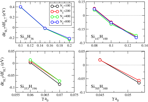
The curvature for the different NCs, estimated from a forward difference formula with , is plotted as a function of in Fig. 1. The curvature is a decreasing function of and has a node at the optimal value of the range parameter . For each NC the curvature results are shown for several values of the number of stochastic orbitals . We find that the statistical fluctuations near become smaller as the system grows and can be reduced with proper choice of . For example, for the larger system the results near can be converged with only compared to the total number of occupied states for this system which is . The reduction of these fluctuations is partially due to the decrease of itself as the NC size increases (this decrease is shown in the right panel of Fig. 1), leading to a smaller contribution of the non-local exchange to the orbital energies.
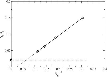
The results in the right panel of the figure also show that closely follows a linear function of . We expect that for larger NCs with , this linear relation will break down and the optimal range parameter will converge to the bulk value, which through reverse engineering Eisenberg and Baer (2009) can be estimated as (shown as a horizontal dotted line). Such a localization-induced by the exchange has been seen for 1D conjugated polymers Vlček et al. (2015) but not for bulk solids like silicon, likely due to the enormity of the calculation.
In Fig. 2 we plot the highest occupied molecular orbital (HOMO, left panel) and lowest unoccupied molecular orbital (LUMO, right panel) energies obtained from the relations Janak (1978)
| (22) |
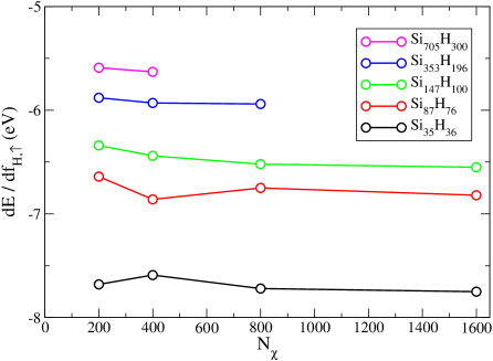
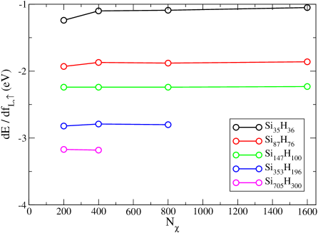
respectively, as a function of at . We find that determining the HOMO and LUMO energies using the above first derivative relations reduces the noise compared to obtaining their values directly from the eigenvalues. Clearly and converge as increases. Moreover, as the system size increases the fluctuations in and decreases for a given value of , consistent with the discussion above. This is evident from the plot of the differences between the frontier orbital energies at adjacent values of .
=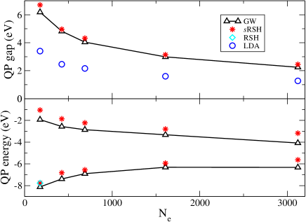
In the lower panel of Fig. 3 we plot the converged (with respect to ) HOMO and LUMO energies at for the series of silicon NCs. For the smallest system () we compare the stochastic approach developed here with a deterministic RSH calculation using a non-local exchange with all occupied orbitals and obtaining the Coulomb convolution integrals with FFTs, thereby eliminating any source of statistical error. The purpose it to show that when the stochastic results are converged the agreement with a deterministic calculations is perfect on a relevant magnitude of energy. We find that the HOMO energy increases and the LUMO energy decreases with the size of the NC. This is consistent with our recent calculations on silicon NCs using the stochastic GW approach, albeit the fact that there is a small shift in the quasi-particle energies obtained from the stochastic RSH approach compared to the sGW. Indeed, a similar shift has been reported previously for much smaller silicon NCs.Stein et al. (2010) However, the source of this discrepancy is not clear, particularly, since the GW calculations were done within the so called limit, and the OT-RSH often provides better quasiparticle energies in comparison to experiments.Kronik et al. (2012) In the upper panel of Fig. 3 we plot the fundamental (quasiparticle) gaps. Here, the agreement with the sGW approach is rather remarkable, especially compared to the LDA results which significantly underestimate the quasiparticle gap across all sizes studied.
| System | Functional | |||||
|---|---|---|---|---|---|---|
| S | LDA | - | -6.13 | -2.73 | 3.40 | 1.6 |
| BN | 800 | -7.72 | -1.09 | 6.63 | 16 | |
| 1600 | -7.75 | -1.05 | 6.70 | 30 | ||
| S | LDA | - | -5.13 | -3.85 | 1.28 | 132 |
| BN | 200 | -5.59 | -3.18 | 2.41 | 234 | |
| 400 | -5.63 | -3.17 | 2.46 | 310 |
(a)
(b)
(c) In CPU-hrs
In Table 1 we provide numerical details of the calculations for the smallest and largest NC studied. We report the results for the HOMO and LUMO orbital energies for two different choices of Comparing these two values we can conclude that the statistical errors for the LUMO are very small ( eV) for the largest NC and even the HOMO has small errors of around eV. Moreover, similar or even larger statistical errors are observed for the smaller NC for much larger values of , indicating that for a given accuracy the number of stochastic orbitals decreases with the system size. This is partially correlated with the reduction of with the system size, as discussed above.
V Summary
We have developed a stochastic representation for the non-local exchange operator in order to combine real-space/plane-waves methods with optimally-tuned range-separated hybrid functionals within the generalized Kohn-Sham scheme. Our formalism uses two principles, one is a stochastic decomposition the Coulomb convolution integrals and the other is the representation of the density matrix using stochastic orbitals. Combining these two ideas leads to a significant reduction of the computational effort and, for the systems studied in this work, to a reduction of the computational scaling of the non-local exchange operator, at the price of introducing a statistical error. The statistical error is controlled by increasing the number of stochastic orbitals and is also found to reduce with the system size Applications to silicon NCs of varying sizes show relatively good agreement for the band-edge quasiparticle excitations in comparison to a many-body perturbation approach within the sGW approximation and excellent agreement for the fundamental band gap. The stochastic approach has a major advantage over the GW by providing a self-consistent Hamiltonian which is central for post-processing, for example in conjunction with a real-time Bethe–Salpeter approach.Rabani et al. (2015) The results shown here for and are the largest reported so far for the optimally-tuned range-separated generalized Kohn-Sham approach.
Acknowledgements.
R. B. and E. R. gratefully thank the Israel Science Foundation–FIRST Program (Grant No. 1700/14). R.B. gratefully acknowledges support for his sabbatical visit by the Pitzer Center and the Kavli Institute of the University of California, Berkeley. D. N. and E. R. acknowledge support by the NSF, grants CHE-1112500 and CHE-1465064, respectively.
Appendix A treatment of the term
For accelerating convergence, it turns out to be better to remove the term from the the random vector expression representing the interaction, i.e.,
This is because in practice the term is very large. Analytically, this term is easily shown to commute with the Fock Hamiltonian and simply contribute a constant (times the occupation) to the eigenvalues and to the total energy, so it can be added a-posteriori:
where
References
- Kohn and Sham (1965) W. Kohn and L. J. Sham, Phys. Rev. 140, A1133 (1965).
- Ogut et al. (1999) S. Ogut, J. R. Chelikowsky, and S. G. Louie, Phys. Rev. Lett. 83, 1270 (1999).
- Godby and White (1998) R. W. Godby and I. D. White, Phys. Rev. Lett. 80, 3161 (1998).
- Teale et al. (2008) A. M. Teale, F. De Proft, and D. J. Tozer, J. Chem. Phys. 129, 044110 (2008).
- Almbladh and von Barth (1985) C.-O. Almbladh and U. von Barth, Phys. Rev. B 31, 3231 (1985).
- Perdew et al. (1982) J. P. Perdew, R. G. Parr, M. Levy, and J. L. Balduz, Phys. Rev. Lett. 49, 1691 (1982).
- Sham and Schlüter (1983) L. J. Sham and M. Schlüter, Phys. Rev. Lett. 51, 1888 (1983).
- Hedin (1965) L. Hedin, Phys. Rev. 139, A796 (1965).
- Hybertsen and Louie (1985) M. S. Hybertsen and S. G. Louie, Phys. Rev. Lett. 55, 1418 (1985).
- Del Sole et al. (1994) R. Del Sole, L. Reining, and R. Godby, Phys. Rev. B 49, 8024 (1994).
- Steinbeck et al. (1999) L. Steinbeck, A. Rubio, L. Reining, M. Torrent, I. White, and R. Godby, Comput. Phys. Commun. 125, 05 (1999).
- Fleszar (2001) A. Fleszar, Phys. Rev. B 64 (2001).
- Onida et al. (2002) G. Onida, L. Reining, and A. Rubio, Rev. Mod. Phys. 74, 601 (2002).
- Rinke et al. (2005) P. Rinke, A. Qteish, J. Neugebauer, C. Freysoldt, and M. Scheffler, New J. Phys. 7, (2005).
- Friedrich and Schindlmayr (2006) C. Friedrich and A. Schindlmayr, NIC Series 31, 335 (2006).
- Shishkin and Kresse (2007) M. Shishkin and G. Kresse, Phys. Rev. B 75, 235102 (2007).
- Trevisanutto et al. (2008) P. E. Trevisanutto, C. Giorgetti, L. Reining, M. Ladisa, and V. Olevano, Phys. Rev. Lett. 101, 226405 (2008).
- Rostgaard et al. (2010) C. Rostgaard, K. W. Jacobsen, and K. S. Thygesen, Phys. Rev. B 81, 085103 (2010).
- Liao and Carter (2011) P. Liao and E. A. Carter, Phys. Chem. Chem. Phys. 13, 15189 (2011).
- Blase et al. (2011) X. Blase, C. Attaccalite, and V. Olevano, Phys. Rev. B 83, 115103 (2011).
- Tamblyn et al. (2011) I. Tamblyn, P. Darancet, S. Y. Quek, S. A. Bonev, and J. B. Neaton, Phys. Rev. B 84, 201402 (2011).
- Samsonidze et al. (2011) G. Samsonidze, M. Jain, J. Deslippe, M. L. Cohen, and S. G. Louie, Phys. Rev. Lett. 107, 186404 (2011).
- Marom et al. (2012) N. Marom, F. Caruso, X. Ren, O. T. Hofmann, T. Körzdörfer, J. R. Chelikowsky, A. Rubio, M. Scheffler, and P. Rinke, Phys. Rev. B 86, 245127 (2012).
- van Setten et al. (2012) M. van Setten, F. Weigend, and F. Evers, J. Chem. Theory Comput. 9, 232 (2012).
- Pham et al. (2013) T. A. Pham, H.-V. Nguyen, D. Rocca, and G. Galli, Phys. Rev. B 87, 155148 (2013).
- Seidl et al. (1996) A. Seidl, A. Görling, P. Vogl, J. A. Majewski, and M. Levy, Phys. Rev. B 53, 3764 (1996).
- Heyd et al. (2005) J. Heyd, J. E. Peralta, G. E. Scuseria, and R. L. Martin, J. Chem. Phys. 123, 174101 (2005).
- Gerber et al. (2007) I. C. Gerber, J. G. Angyan, M. Marsman, and G. Kresse, J. Chem. Phys. 127, 054101 (2007).
- Brothers et al. (2008) E. N. Brothers, A. F. Izmaylov, J. O. Normand, V. Barone, and G. E. Scuseria, J. Chem. Phys. 129, 011102 (2008).
- Barone et al. (2011) V. Barone, O. Hod, J. E. Peralta, and G. E. Scuseria, Acc. Chem. Res. 44, 269 (2011).
- Savin and Flad (1995) A. Savin and H. J. Flad, Int. J. Quantum Chem. 56, 327 (1995).
- Iikura et al. (2001) H. Iikura, T. Tsuneda, T. Yanai, and K. Hirao, J. Chem. Phys. 115, 3540 (2001).
- Yanai et al. (2004) T. Yanai, D. P. Tew, and N. C. Handy, Chem. Phys. Lett. 393, 51 (2004).
- Baer and Neuhauser (2005) R. Baer and D. Neuhauser, Phys. Rev. Lett. 94, 043002 (2005).
- Livshits and Baer (2007) E. Livshits and R. Baer, Phys. Chem. Chem. Phys. 9, 2932 (2007).
- Vydrov and Scuseria (2006) O. A. Vydrov and G. E. Scuseria, J. Chem. Phys. 125, 234109 (2006).
- Chai and Head-Gordon (2008) J. D. Chai and M. Head-Gordon, Phys. Chem. Chem. Phys. 10, 6615 (2008).
- Livshits and Baer (2008) E. Livshits and R. Baer, J. Phys. Chem. A 112, 12789 (2008).
- Baer et al. (2010) R. Baer, E. Livshits, and U. Salzner, Annu. Rev. Phys. Chem. 61, 85 (2010).
- Stein et al. (2010) T. Stein, H. Eisenberg, L. Kronik, and R. Baer, Phys. Rev. Lett. 105, 266802 (2010).
- Kronik et al. (2012) L. Kronik, T. Stein, S. Refaely-Abramson, and R. Baer, J. Chem. Theory Comput. 8, 1515 (2012).
- Körzdörfer et al. (2012) T. Körzdörfer, R. M. Parrish, N. Marom, J. S. Sears, C. D. Sherrill, and J.-L. Brédas, Phys. Rev. B 86, 205110 (2012).
- Jacquemin et al. (2014) D. Jacquemin, B. Moore, A. Planchat, C. Adamo, and J. Autschbach, J. Chem. Theory Comput. 10, 1677 (2014).
- Stein et al. (2012) T. Stein, J. Autschbach, N. Govind, L. Kronik, and R. Baer, J. Phys. Chem. Lett. 3, 3740 (2012).
- Neuhauser et al. (2014a) D. Neuhauser, Y. Gao, C. Arntsen, C. Karshenas, E. Rabani, and R. Baer, Phys. Rev. Lett. 113, 076402 (2014a).
- Baer et al. (2013) R. Baer, D. Neuhauser, and E. Rabani, Phys. Rev. Lett. 111, 106402 (2013).
- Neuhauser et al. (2014b) D. Neuhauser, R. Baer, and E. Rabani, J. Chem. Phys. 141, 041102 (2014b).
- Baer and Rabani (2012) R. Baer and E. Rabani, Nano Lett. 12, 2123 (2012).
- Neuhauser et al. (2013a) D. Neuhauser, E. Rabani, and R. Baer, J. Chem. Theory Comput. 9, 24 (2013a).
- Neuhauser et al. (2013b) D. Neuhauser, E. Rabani, and R. Baer, J. Phys. Chem. Lett. 4, 1172 (2013b).
- Ge et al. (2013) Q. Ge, Y. Gao, R. Baer, E. Rabani, and D. Neuhauser, J. Phys. Chem. Lett. 5, 185 (2013).
- Gao et al. (2015) Y. Gao, D. Neuhauser, R. Baer, and E. Rabani, J. Chem. Phys. 142, 034106 (2015).
- Baer and Neuhauser (2012) R. Baer and D. Neuhauser, J. Chem. Phys. 137, 051103 (2012).
- Cytter et al. (2014) Y. Cytter, D. Neuhauser, and R. Baer, J. Chem. Theory Comput. 10, 4317 (2014).
- Rabani et al. (2015) E. Rabani, R. Baer, and D. Neuhauser, Phys. Rev. B 91, 235302 (2015).
- Kosloff (1988) R. Kosloff, J. Phys. Chem. 92, 2087 (1988).
- Kosloff (1994) R. Kosloff, Annu. Rev. Phys. Chem. 45, 145 (1994).
- Savin (1995) A. Savin, Beyond the Kohn-Sham Determinant (World Scientific, Singapore, 1995), p. 129.
- Dreizler and Gross (1990) R. M. Dreizler and E. K. U. Gross, Density Functional Theory: An Approach to the Quantum Many Body Problem (Springer, Berlin, 1990).
- Stein et al. (2009) T. Stein, L. Kronik, and R. Baer, J. Am. Chem. Soc. 131, 2818 (2009).
- Janak (1978) J. Janak, Phys. Rev. B 18, 7165 (1978).
- Eisenberg and Baer (2009) H. R. Eisenberg and R. Baer, Phys. Chem. Chem. Phys. 11, 4674 (2009).
- Kosloff and Kosloff (1983) D. Kosloff and R. Kosloff, J. Comput. Phys. 52, 35 (1983).
- Zhou et al. (2006) Y. Zhou, Y. Saad, M. L. Tiago, and J. R. Chelikowsky, Phys. Rev E 74, 066704 (2006).
- Khoo et al. (2010) K. Khoo, M. Kim, G. Schofield, and J. R. Chelikowsky, Phys. Rev. B 82, 064201 (2010).
- Vlček et al. (2015) V. Vlček, H. R. Eisenberg, G. Steinle-Neumann, and R. Baer, arXiv preprint arXiv:1509.05222 (2015).