Time-delayed models of gene regulatory networks

Abstract

In this review we discuss different mathematical models of gene regulatory networks as relevant to the onset and development of cancer. After discussion of alternative modelling approaches, we use a paradigmatic two-gene network to focus on the role played by time delays in the dynamics of gene regulatory networks. We contrast the dynamics of the reduced model arising in the limit of fast mRNA dynamics with that of the full model. The review concludes with the discussion of some open problems.

1 Introduction

Cancer is a complex disease, triggered by multiple mutations in various genes and exacerbated by a number of different behavioural and environmental factors. Some risk factors associated with possible onset and development of cancer are preventable, such as, inappropriate diet, physical inactivity, smoking and drinking [1], while other causes include pathogens (HPV16 and HPV18 are known to cause up to 70% of cervical cancer cases [2]), as well as genetic pre-disposition. Many studies have focussed on identifying efficient genetic cancer biomarkers, such as, specific genes and groups of genes associated with significant number of cases of breast cancer [3], prostate [4] and pancreatic cancer [5]. Despite this progress, due to significant complexity associated with mutations of various cancer genes, many molecular mechanisms of oncogenesis remain poorly understood.

Recent advances in microarray and high-throughput sequencing technologies have provided pathways for measuring the expression of thousands of genes and mapping most crucial genes and groups of genes controlling different types of cancer. The networks of interactions between DNA, RNA, proteins and molecules, are defined as gene regulatory networks (GRNs). GRNs play a major role in a large number of normal life processes, including cell differentiation, metabolism, the cell cycle and signal transduction, hence, significant efforts have been made to develop mathematical techniques for their analysis [6, 7, 8].

GRNs are usually formalised as networks (undirected or directed) where the nodes represent individual genes, proteins etc, and the edges correspond to some form of regulation between the nodes. In order to make progress in understanding the onset and development of cancer, as well as to develop effective drug targets, it is essential to be able to reconstruct GRNs pertinent to particular types of cancer from available data. Yeh et al. [9] have used a $K$-nearest-neighbours algorithm to identify GRNs correlated with cancer, tumour grade and stage in prostate cancer. As an alternative approach, Bonnet et al. [10] have utilised LeMoNe (Learning Module Networks) algorithms to derive GRNs from gene and mRNA expression, as measured in lymphoblastoid cell lines of prostate cancer patients. A rule-based algorithm has been successfully used to determine GRNs in colon cancer [11], and similar kinds of networks have been identified from microarray data using neural fuzzy networks [12]. Madhamshettiwar et al. [13] discuss different approaches to infer GRNs in ovarian cancer, as well as the potential of using these GRNs to develop optimal drug targets. Bayesian network techniques have been employed to construct GRNs from microarray data for breast cancer [14]. In a recent paper, Emmert-Streib et al. [15] have successfully used a BC3Net inference algorithm to analyse a large-scale breast cancer gene expression data set and reconstruct the associated GRN.

In the next section we survey and compare different approaches to model the dynamics of GRNs, making an emphasis on particular biological features that can be best represented by each of the methods. Section 3 focuses on the role of transcriptional and translational time delays in GRN models, and we show how such delays can be introduced in a paradigmatic two-gene activator-inhibitor GRN. Depending on a particular biological regime in which a given GRN is operating, it is often possible to encounter a situation where there is a significant separation of time scales due to, for instance, very fast mRNA dynamics compared to other characteristic time scales. In such a case it is possible to perform dimensional reduction and concentrate on the dynamics of a smaller number of variables. In Section 4 we analyse such reduced model and show how one can derive analytical conditions that lead to a transition from a stable steady state to stable periodic oscillations that are impossible in the model system without the time delays. Section 5 extends the analysis to a full nonlinear system to illustrate differences in stability conditions. The review concludes in Section 6 with a discussion of main results and some open questions.

2 Mathematical models of gene regulatory networks

In the analysis of gene regulatory networks and their dynamics, the first step is the identification of key modules or components and possible relations between them, which is often done by interrogating available expression data. Once the topology of the GRN has been fixed, the next step in modelling the dynamics is making realistic assumptions about specific rules that govern the expression of particular genes. Depending on the level of understanding of underlying processes, the complexity of the GRN under investigation, and the specific questions to be addressed, there are several methodologically different approaches that can be employed. Endy & Brent [16] and Hasty et al. [17] discuss biological underpinnings for studying and modelling GRNs, while excellent reviews by de Jong [7], Bernot et al. [8], Tušek & Kurtanjek [18], and Hecker et al. [19] give an overview of mathematical and statistical techniques that have been successfully used to model GRNs, and some of these methods are discussed below.

2.1 Boolean networks

Some of the first models developed for modelling GRNs were the so-called Boolean networks [20, 21, 22], where the states of all genes participating in the interactions are represented by binary variables having the values of ON and OFF, or 1 and 0, with the possibility of either synchronous or asynchronous update rules for the nodes. Boolean logic rules are then used to approximate regulatory control of gene expression [23], with updates of binary states of all genes taking place simultaneously [24]. Boolean networks approach has been extended in several directions to provide a better approximation of real GRNs. Shmulevich et al. [25] have proposed a probabilistic analogue of Boolean networks to account for stochastic nature of many processes involved in gene expression. Silvescu and Honavar [26] have proposed temporal Boolean networks, where the next state of genes in the networks is determined not only by their current state, but also by a fixed number of their previous states, which effectively allows one to take into account some history of transitions in a GRN. Recently, Boolean network models of GRNs have been compared to models based on ordinary differential equations (ODEs), and, in fact, it has been shown that some Boolean models can be rigorously derived as coarse-grained analogues of some ODE models [27].

Significant advantage of using Boolean networks to model GRNs lies in the fact that they allow one to consider networks with a very large number of nodes. At the same time, there are several deficiencies in this approach. The first one concerns the fact that since the gene states only admit the values of ON or OFF, this formalism does not take into account intermediate stages of gene expression [28]. Another issue is that GRNs modelled by Boolean networks can exhibit behaviour not observed in real life, hence, special care has to be taken when choosing the class of admissible Boolean functions [29].

2.2 Fuzzy methods

Due to intrinsic imprecision and uncertainty associated with gene expression data, it may be appropriate to move away from precise rules of Boolean logic in favour of machine learning techniques based on fuzzy logic. The basic idea is that rather than trying to reconstruct some assumed fixed gene network topology, one considers the whole family of possible networks with all possible distributions of links between nodes. The problem lies in using actual data to assign appropriate probabilities to each of these configurations, so that for a given input the fuzzy network would provide an output that most resembles actual data. A significant advantage of fuzzy logic for inferring the structure of GRNs lies in their ability to rely on already available knowledge of biological relations between different nodes in the network, and, at the same time, being able to recover important previously unknown connections. On the other hand, fuzzy methods for GRN inference are characterised by a high level of computational complexity.

To give a few examples, fuzzy approach has been used to analyse microarray data from the yeast cell cycle and to recover a set of GRNs, with $k$-nearest-neighbour algorithm being used to replace missing data [30]. Woolf and Wang [31] have used a $k$-means clustering algorithm to reconstruct and evaluate GRNs for Saccharomyces cerevisiae. In this approach, groups of co-regulated genes are considered as clusters, and clustering algorithm is then used to detect cluster centres. Volkert and Mahlis [32] have used a smooth response surface algorithm to recover GRNs from gene expression data for Saccharomyces cerevisiae. Approaches based on an artificial bee colony search algorithm have allowed the reconstruction of a GRN in Escherichia coli [33]. A very recent review by Al Qazlan et al. [34] gives an overview of different fuzzy methods, as well as their combinations with other approaches, such as ordinary differential equations, with the purpose of optimising data mining of gene expression and microarray datasets to recover GRNs.

2.3 Ordinary and delay differential equation models

A very powerful and mathematically insightful methodology for analysis of GRNs is based on nonlinear ordinary or delay differential equations (ODEs or DDEs). In this approach, a gene regulatory network is represented by concentrations of different mRNAs and proteins, and the dynamics can be written as a system of ODEs or DDEs using the law of mass action for individual reactions [6]. Some of the earliest results on ODE models of gene regulation go back to Goodwin [35, 36], who introduced and studied a negative feedback loop involving the concentrations of mRNA, an enzyme and a metabolite. It has been later shown that a negative feedback loop is absolutely essential to ensure the existence of stable periodic solutions, while positive feedback is required for multi-stationarity [37, 38]. This approach was subsequently generalised and expanded [39, 40, 41, 42]; reviews by Smolen et al. [24], de Jong [7] and Hecker et al. [19] discuss some of these models based on systems of nonlinear ODEs. A very important aspect of all these models is a regulation function that controls the rates of gene expression. In light of experimental evidence suggesting monotonic sigmoidal shape of regulation functions [43], a conventional choice for this function is given by the Hill function [44, 45, 46]. Weiss [47] has discussed various chemical mechanisms associated with the Hill function, including different kinds of ligand binding, and a more recent review of the uses of the Hill function in GRN models can be found in [48].

In order to more accurately represent a switch-like behaviour of the gene expression, several authors have developed models of GRNs using piecewise-linear differential equations, in which the continuous Hill function is replaced by a discontinuous step function [49, 50, 51, 52, 53, 54]. Besides regular steady states, the piecewise-linear models also allow for singular steady states, which although important for representing homeostasis in GRNs, are complex to analyse due to discontinuities at the thresholds [55, 56]. Polynikis et al. [44] discuss various features of piecewise-linear ODE models and different dynamical regimes that can be exhibited in these models, including possible periodic solutions, sharp-threshold dynamics, and the comparison with models based on continuous regulation function.

In terms of applications to cancer, ODE models have explained aberrant dynamics of the NF-$\kappa$B transcription factor linked to oncogenesis, tumour progression and resistance to therapy, as well as the dynamics of I$\kappa$B-NF-$\kappa$B [57, 58]. Another example is the analysis of the feedback loop between the tumour suppressor p53 and the oncogene Mdm2 [59], and the single-cell response of p53 to radiation-induced DNA damage [60]. There is a clinical evidence suggesting that different components of the PI3K/AKT pathway can lead to aberrant cell growth, metastatic competence and therapy resistance, and some progress has been made in modelling this pathway and identifying inhibitors responsible for the regulation of PI3K/AKT signalling [61]. Cheng et al. [62] and Edelman et al. [63] give a number of examples of the uses of differential equation based models for the analysis of GRNs in cancer.

Another aspect that has to be properly accounted for in dynamical models is the fact that transcription and translation during gene expression often take place over non-negligible time periods. Monk [64] has shown how time delays can cause oscillatory gene expression and provide insights into the dynamics of interactions between p53 and Mdm2 proteins associated with cancer suppression. Subsequent research has focused on the role of time delays in GRN dynamics [65, 66, 67, 68, 69]. Xiao and Cao [70] have analysed a Hopf bifurcation in a gene network with two transcriptional delays, which occurs when the sum of the delays passes through a critical value, and shown how the amplitude and period of oscillations of gene expression change with the time delays. Due to the fact that it may not be practically possible to identify discrete transcription/translation time delays, a better alternative would be to use models with distributed delay [71]. Models with time delays have been used to understand the regulation of feedback loops involving transcription factors E2F and Myc, known oncogenes and possible tumour suppressors [72, 73]. Ribeiro et al. [74] have developed a delayed stochastic simulation algorithm for analysis of the p53-Mdm2 feedback loop whose malfunction is associated with 50% of cancers. Sequences of multiple reactions with unknown intermediate kinetics can also be successfully analysed using time-delayed models [75, 76].

2.4 Stochastic models

Experimental evidence suggests that significant stochastic fluctuations are observed during gene expression and regulation, hence, in many cases it is paramount to use stochastic models for studying GRN dynamics [77, 78]. Even in the absence of extrinsic noise associated with variability in different environmental factors, there are several fundamental processes responsible for intrinsic stochasticity of gene expression [79, 80]. One of these is the process of initiation of transcription, which starts by first forming an elongation complex by binding RNA polymerase (RNAp) to the promoter region of the gene, and there is a significant variation in the duration of elongation processes between different transcription events [81, 82, 83, 84]. Binding of RNAp to the promoter regions of different genes results in switching of these genes on and off, thus either blocking or facilitating further transcription, which gives another major source of noise in GRNs. Stochasticity in expression of individual gene results in stochastic behaviour of larger genetic circuits and GRNs [77, 85]. Some of the early work on stochastic gene expression emerged from experiments in synthetic biology [86, 87] that demonstrated how stochasticity can result in sustained oscillations, and significant amount of research has been subsequently done both theoretically and experimentally on the analysis of stochastic (and delayed) oscillations in gene regulatory networks [80, 88, 89, 90]. Zavala and Marquez-Lago have recently considered delay-induced oscillations in deterministic and stochastic models of single-cell gene expression, highlighting important differences between these two types of models and associated behaviours [91].

Besides being an intrinsic feature of biological dynamics, stochasticity has proved to be important in the context of engineered genetic switches [86, 92]. de Jong [7] and El Samad et al. [93] discuss various methods for modelling stochastic GRN models, including stochastic master equation and various stochastic simulation algorithms. Bratsun et al. [90] have developed an algorithm for analysis of non-Markovian dynamics in GRNs with time delays and showed that these delays are able to induce oscillatory dynamics in the case where deterministic models do not exhibit oscillations. This methodology was later improved, and several exact stochastic simulation algorithms have been developed for simulations of time-delayed models [94, 95]. A review by Ribeiro [84] discusses various techniques for simulating stochastic time-delayed dynamics of gene expression, and very recently Jansen et al. [96] have reviewed the role of delay distribution in the stochastic dynamics during gene expression.

Another way to approach stochasticity in the analysis and reconstruction of GRNs is by using so-called Bayesian networks [97], where gene expression values are represented as random variables, and relations between them are probabilistic. Learning techniques for Bayesian networks [98, 99] allow one to combine expression data with an a priori knowledge to deduce the structure of GRN that best matches the available expression data. Friedman et al. [97] have developed an algorithm for deriving Bayesian networks that circumvents a dimensionality problem, and this method has been used to analyse the cell cycle data for S. cerevisiae containing numerous measurements of mRNA expression levels [100]. Out of 800 genes it was possible to identify a few genes controlling the regulation of cell cycle processes.

The rest of this paper is devoted to consideration of the effects of transcriptional and translational time delays on the dynamics of GRNs. In the next Section we introduce the time-delayed model of a two-gene activation-inhibition network together with its quasi-steady state simplification, and establish the well-posedness of both models. Section 4 contains the derivation of analytical conditions for stability and a Hopf bifurcation in the case of very fast mRNA dynamics, while in Section 5 the analysis is extended to the full time-delayed system. The paper concludes in Section 6 with discussion of results and future research directions.

3 Time-delayed models: derivation and positivity

To motivate the analysis of time-delayed effects in gene regulatory dynamics, following Polynikis et al. [44], we consider an activation-inhibition two-gene GRN consisting of two genes $a$ and $b$, which are assumed to have no effect on their own expression; at the same time, protein $P_{b}$ is assumed to activate the expression of gene $a$, while protein $P_{a}$ inhibits the expression of gene $b$. This is one of the fundamental motifs, which has been shown to be functionally relevant in GRNs [62, 101]. Denoting the concentrations of proteins $P_{a}$ and $P_{b}$ as $p_{a}$ and $p_{b}$, and concentrations of transcribed mRNAs as $r_{a}$ and $r_{b}$, the following system of equations can be derived for the dynamics of this GRN [44]

$$\begin{array}[]{l}\dot{r}_{a}=m_{a}h^{+}(p_{b};\theta_{b},n_{b})-\gamma_{a}r_{a},\\ \\ \dot{r}_{b}=m_{b}h^{-}(p_{a};\theta_{a},n_{a})-\gamma_{b}r_{b},\\ \\ \dot{p}_{a}=k_{a}r_{a}-\delta_{a}p_{a},\\ \\ \dot{p}_{b}=k_{b}r_{b}-\delta_{b}p_{b},\end{array}$$ (1)

where $m_{i}$ are the maximum transcription rates, $k_{i}$ are the translation rates, $\gamma_{i}$ are the mRNA degradation rates, and $\delta_{i}$ are the protein degradation rates for $i=a,b$. Equations (1) are called the complete nonlinear model (CNM). To make further analytical progress, the activation and inhibition functions in the system (1) can be written as the following Hill functions,

$$\begin{array}[]{l}\displaystyle{h^{+}(p_{i};\theta_{i},n_{i})=\frac{p_{i}^{n_{i}}}{p_{i}^{n_{i}}+\theta_{i}^{n_{i}}},\mbox{ and }}\\ \\ \displaystyle{h^{-}(p_{i};\theta_{i},n_{i})=1-h^{+}(p_{i};\theta_{i},n_{i})=\frac{\theta_{i}^{n_{i}}}{p_{i}^{n_{i}}+\theta_{i}^{n_{i}}},\hskip 14.22636pti=a,b,}\end{array}$$

where $\theta_{a}$ and $\theta_{b}$ are known as activation and inhibition coefficients, and the integer parameters $n_{a}$ and $n_{b}$, known as Hill coefficients, determine the steepness of Hill curves [6]. The parameters $\theta_{a}$ and $\theta_{b}$ give the values of protein concentrations $p_{a}$ and $p_{b}$, at which the corresponding Hill function achieves half of its maximum value. Depending on the values of transcription rates, this would then lead to a significant increase in the respective mRNAs regulated by these proteins [8, 44].

Due to the fact that the dynamics of mRNA is normally much faster that that of related proteins, one can use a quasi-steady state assumption to simplify the CNM (1) by reducing the number of equations. Effectively, this means assuming that mRNAs have already reached their steady-state concentrations, i.e. taking $\dot{r}_{i}\approx 0$, $i=a,b$ in the CNM (1), and then focusing on the dynamics of proteins only, as given by the following simplified nonlinear model (SNM)

$$\begin{array}[]{l}\dot{p}_{a}=k^{\prime}_{a}h^{+}(p_{b};\theta_{b},n_{b})-\delta_{a}p_{a},\\ \\ \dot{p}_{b}=k^{\prime}_{b}h^{-}(p_{a};\theta_{a},n_{a})-\delta_{b}p_{b},\end{array}$$

where

$${k^{\prime}_{a}=\frac{m_{a}k_{a}}{\gamma_{a}},\hskip 14.22636ptk^{\prime}_{b}=\frac{m_{b}k_{b}}{\gamma_{b}}.}$$ (2)

Polynikis et al. [44] have shown that, while the CNM exhibits Hopf bifurcation of a positive equilibrium, leading to persistent oscillations, in the case of the SNM model this behaviour can disappear. They have also demonstrated an important role played by the Hill coefficients, as well as the separation of timescales between mRNA and proteins, with a larger scale separation favouring a stable equilibrium rather than oscillatory behaviour.

While the transcription and translation may be faster than characteristic times associated with significant changes in protein concentrations (of the order of 5 minutes for transcription+translation and 1 hour for a 50% change in the concentration of translated protein for E. coli. [6]), these are, in fact, multi-step processes consisting of thousands of consecutive chemical reactions. Hence, the duration of transcription and translation is non-negligible when considered in the context of GRN dynamics [84, 96], and has to be correctly accounted for in mathematical models. To analyse the effects of transcriptional and translational time delays we introduce the following model

$$\begin{array}[]{l}\dot{r}_{a}=m_{a}h^{+}(p_{b}(t-\tau_{r_{a}});\theta_{b},n_{b})-\gamma_{a}r_{a},\\ \\ \dot{r}_{b}=m_{b}h^{-}(p_{a}(t-\tau_{r_{b}});\theta_{a},n_{a})-\gamma_{b}r_{b},\\ \\ \dot{p}_{a}=k_{a}r_{a}(t-\tau_{p_{a}})-\delta_{a}p_{a},\\ \\ \dot{p}_{b}=k_{b}r_{b}(t-\tau_{p_{b}})-\delta_{b}p_{b},\end{array}$$ (3)

where $\tau_{r_{a}}$ and $\tau_{r_{b}}$ are the delays during transcription of mRNAs $r_{a}$ and $r_{b}$, and $\tau_{p_{a}}$ and $\tau_{p_{b}}$ are the delays during translation of proteins $p_{a}$ and $p_{b}$, respectively. This model will be referred to as the delayed complete non-linear model (DCNM). Similar to the case of instantaneous transcription and translation, the quasi-steady-state assumption simplifies the system (3) to the following delayed simplified non-linear model (DSNM)

$$\begin{array}[]{l}\dot{p}_{a}=k^{\prime}_{a}h^{+}(p_{b}(t-\tau_{r_{a}}-\tau_{p_{a}});\theta_{b},n_{b})-\delta_{a}p_{a},\\ \\ \dot{p}_{b}=k^{\prime}_{b}h^{-}(p_{a}(t-\tau_{r_{b}}-\tau_{p_{b}});\theta_{a},n_{a})-\delta_{b}p_{b},\end{array}$$ (4)

with parameters $k^{\prime}_{a}$ and $k^{\prime}_{b}$ defined in (2).

Before proceeding with the analysis, one has to augment the models (3) and (4) with the appropriate initial conditions and establish that these models are well-posed, i.e. that their solutions remain non-negative for all time to ensure their biological feasibility. The initial conditions for the DCNM model (3) are given by

$$\begin{array}[]{l}r_{a}(s)=\phi_{1}(s),\hskip 14.22636pts\in[-\tau_{\rm max},0],\\ \\ r_{b}(s)=\phi_{2}(s),\hskip 14.22636pts\in[-\tau_{\rm max},0],\\ \\ p_{a}(s)=\phi_{3}(s),\hskip 14.22636pts\in[-\tau_{\rm max},0],\\ \\ p_{b}(s)=\phi_{4}(s),\hskip 14.22636pts\in[-\tau_{\rm max},0],\\ \\ \end{array}$$ (5)

where $\tau_{\rm max}=\max(\tau_{r_{a}},\tau_{r_{b}},\tau_{p_{a}},\tau_{p_{b}})$ and $\phi_{i}(s)\in C([-\tau_{\rm max},0],\mathbb{R})$ with $\phi_{i}(s)\geq 0$ $(-\tau_{\rm max}\leq s\leq 0$, $i=1,..,4)$, and similarly for the DSNM model (4). Here, $C([-\tau_{\rm max},0],\mathbb{R})$ is the Banach space of continuous mappings of the interval $[-\tau_{\rm max},0]$ onto $\mathbb{R}$. It is further assumed that $r_{a}(0)>0$, $r_{b}(0)>0$ to ensure that at least some amount of proteins will be produced.

We now prove that the solution $(r_{a}(t),r_{b}(t),p_{a}(t),p_{b}(t))$ of the DCNM model (3) with the initial condition (5) is positive for all $t>0$. This result can be proven by contradiction, following the methodology used in [102]. As a first step, let us show that $r_{b}(t)\geq 0$ for all $t>0$. Let $t_{1}>0$ be the first time when $p_{a}(t_{1})r_{b}(t_{1})=0$; assuming that $r_{b}(t_{1})=0$ implies $p_{a}(t)\geq 0$ for all $t\in[0;t_{1}]$, and since $t_{1}$ is the first time when $r_{b}(t_{1})=0$, this also means $dr_{b}(t_{1})/dt\leq 0$, i.e. the function $r_{b}(t)$ is decreasing at $t=t_{1}$. On the other hand, evaluating the second equation of the system (3) at $t=t_{1}$ yields

$$\frac{dr_{b}(t_{1})}{dt}=\frac{m_{b}\theta_{a}^{n_{a}}}{p_{a}(t_{1}-\tau_{r_{b}})^{n_{a}}+\theta_{a}^{n_{a}}}>0,$$

which gives a contradiction. Since $r_{b}(0)>0$, this implies $r_{b}(t)>0$ for all $t>0$. Now that the positivity of $r_{b}(t)$ has been established, let $t_{2}>0$ be the first time when $p_{b}(t_{2})=0$. In order for this to happen, one must have $dp_{b}(t_{2})/dt\leq 0$, i.e. the function $p_{b}(t)$ should be decreasing at $t=t_{2}$. At the same time, evaluating the last equation of the system (3) at $t=t_{2}$ yields

$$\frac{dp_{b}(t_{2})}{dt}=k_{b}r_{b}(t_{2}-\tau_{p_{b}})>0,$$

which gives a contradiction, and, therefore, $p_{b}(t)>0$ for all $t>0$. In a similar manner, the positivity of $p_{b}(t)$ implies the positivity of $r_{a}(t)$, which in turn implies the positivity of $p_{a}(t)$. Hence, all solutions $r_{a}(t)$, $r_{b}(t)$, $p_{a}(t)$ and $p_{b}(t)$ of the DCNM model (3) are positive for all $t>0$. The same approach can be employed to show positivity of solutions of the DSNM model (4).

Steady states $(\bar{r}_{a},\bar{r}_{b},\bar{p}_{a},\bar{p}_{b})$ of the DCNM model can be found as roots of the following system of algebraic equations

$$\begin{array}[]{l}m_{a}h^{+}(\bar{p}_{b};\theta_{b},n_{b})-\gamma_{a}\bar{r}_{a}=0,\\ \\ m_{b}h^{-}(\bar{p}_{a};\theta_{a},n_{a})-\gamma_{b}\bar{r}_{b}=0,\\ \\ k_{a}\bar{r}_{a}-\delta_{a}\bar{p}_{a}=0,\\ \\ k_{b}\bar{r}_{b}-\delta_{b}\bar{p}_{b}=0.\end{array}$$

This gives

$${\bar{r}_{a}=\frac{\delta_{a}}{k_{a}}\bar{p}_{a},\hskip 14.22636pt\bar{r}_{b}=\frac{\delta_{b}}{k_{b}}\bar{p}_{b},\hskip 14.22636pt\bar{p}_{b}=\frac{\phi_{b}\theta^{n_{a}}_{a}}{\theta^{n_{a}}_{a}+\bar{p}^{n_{a}}_{a}},}$$

where $\bar{p}_{a}$ satisfies the polynomial equation

$${\theta^{n_{b}}_{b}\sum_{k=0}^{n_{b}}\binom{n_{b}}{k}\bar{p}^{n_{a}(n_{b}-k)+1}_{a}\theta^{n_{a}k}_{a}+(\bar{p}_{a}-\phi_{a})(\phi_{b}\theta^{n_{a}}_{a})^{n_{b}}=0,}$$ (6)

and we used the notation

$${\phi_{a}=\frac{m_{a}k_{a}}{\gamma_{a}\delta_{a}},\hskip 14.22636pt\phi_{b}=\frac{m_{b}k_{b}}{\gamma_{b}\delta_{b}}.}$$

Even for realistically small values of Hill coefficients, such as $n=2,3$ [103] or $n=4$-$8$ [104], the equation (6) is too complicated to allow one to analytically find closed form expressions for $\bar{p}_{a}$ and other state variables. Despite not having explicit formulae for possible steady states $(\bar{r}_{a},\bar{r}_{b},\bar{p}_{a},\bar{p}_{b})$, one can still perform the analysis of stability in terms of system parameters, and such results would be valid for the values of steady state variables that can be accurately and efficiently determined through numerical solution of the polynomial equation (6).

4 Analysis of the delayed simplified non-linear model (DSNM)

In order to gain some first insights into the role of transcriptional and translational delays on the dynamics of GRN, we focus on the behaviour of the delayed simplified non-linear model (DSNM) (4). To reduce the number of free parameters in the model, we introduce the new variables

$$\hat{p}_{a}(t)=p_{a}(t),\quad\hat{p}_{b}(t)=p_{b}(t-\tau_{r_{a}}-\tau_{p_{a}}),$$ (7)

which transform the first equation of the system (4) into

$$\dot{p}_{a}=k^{\prime}_{a}h^{+}(p_{b}(t-\tau_{r_{a}}-\tau_{p_{a}});\theta_{b},n_{b})-\delta_{a}p_{a}\quad\Longleftrightarrow\quad\dot{\hat{p}}_{a}(t)=k^{\prime}_{a}h^{+}(\hat{p}_{b}(t);\theta_{b},n_{b})-\delta_{a}\hat{p}_{a}(t).$$

The second equation of the system (4) evaluated at $t-\tau_{r_{a}}-\tau_{p_{a}}$ has the form

$$\dot{p}_{b}(t-\tau_{r_{a}}-\tau_{p_{a}})=k^{\prime}_{b}h^{-}(p_{a}(t-\tau_{r_{a}}-\tau_{p_{a}}-\tau_{r_{b}}-\tau_{p_{b}});\theta_{a},n_{a})-\delta_{b}p_{b}(t-\tau_{r_{a}}-\tau_{p_{a}}),$$

and in terms of the new variables (7) this can be rewritten as

$$\dot{\hat{p}}_{b}(t)=k^{\prime}_{b}h^{-}(\hat{p}_{a}(t-\tau_{r_{a}}-\tau_{p_{a}}-\tau_{r_{b}}-\tau_{p_{b}});\theta_{a},n_{a})-\delta_{b}\hat{p}_{b}(t).$$

Thus, the system (4) takes a form

$$\begin{array}[]{l}\dot{\hat{p}}_{a}(t)=k^{\prime}_{a}h^{+}(\hat{p}_{b}(t);\theta_{b},n_{b})-\delta_{a}\hat{p}_{a}(t),\\ \\ \dot{\hat{p}}_{b}(t)=k^{\prime}_{b}h^{-}(\hat{p}_{a}(t-\tau);\theta_{a},n_{a})-\delta_{b}\hat{p}_{b}(t),\end{array}$$ (8)

where

$$\tau=\tau_{r_{a}}+\tau_{p_{a}}+\tau_{r_{b}}+\tau_{p_{b}},$$

is the new combined time delay. The equation for characteristic eigenvalues $\lambda$ of the linearisation near a steady state $(\bar{p}_{a},\bar{p}_{b})$ of the system (8) has the form

$$(\lambda+\delta_{a})(\lambda+\delta_{b})+D_{\text{DSNM}}e^{-\lambda\tau}=0,$$ (9)

where

$${D_{\text{DSNM}}=k^{\prime}_{a}k^{\prime}_{b}n_{a}n_{b}\frac{\theta^{n_{a}}_{a}\theta^{n_{b}}_{b}\bar{p}^{(n_{a}-1)}_{a}\bar{p}^{(n_{b}-1)}_{b}}{(\theta^{n_{a}}_{a}+\bar{p}^{n_{a}}_{a})^{2}(\theta^{n_{b}}_{b}+\bar{p}^{n_{b}}_{b})^{2}}=n_{a}n_{b}\delta_{a}\delta_{b}\frac{\bar{p}^{n_{a}}_{a}}{\theta^{n_{a}}_{a}+\bar{p}^{n_{a}}_{a}}\frac{\theta^{n_{b}}_{b}}{\theta^{n_{b}}_{b}+\bar{p}^{n_{b}}_{b}}.}$$

In the limit $\tau=0$, this equation reduces to the quadratic equation [44]

$$\lambda^{2}+(\delta_{a}+\delta_{b})\lambda+\delta_{a}\delta_{b}+D_{\text{DSNM}}=0,$$ (10)

whose roots always have negative real parts, since $\delta_{a}>0$, $\delta_{b}>0$ and $D_{\text{DSNM}}>0$. This implies that for $\tau=0$, the steady state $(\bar{p}_{a},\bar{p}_{b})$ is stable for any values of parameters. To investigate whether this steady state can lose stability for $\tau>0$, one can note that $\lambda=0$ is not a solution of the characteristic equation (9). Hence, the only possible way how the steady state $(\bar{p}_{a},\bar{p}_{b})$ can lose its stability is when a pair of complex conjugate eigenvalues crosses the imaginary axis. In the light of this observation, one can look for eigenvalues of the equation (9) in the form $\lambda=i\omega$ for some real $\omega>0$. Substituting this into Eq. (9) and separating into real and imaginary parts gives

$$\begin{array}[]{l}\omega^{2}-\delta_{a}\delta_{b}=D_{\text{DSNM}}\cos(\omega\tau),\\ \\ (\delta_{a}+\delta_{b})\omega=D_{\text{DSNM}}\sin(\omega\tau).\end{array}$$ (11)

Squaring and adding these two equations yields the following equation for $z=\omega^{2}$

$$h(z)=z^{2}+(\delta_{a}^{2}+\delta_{b}^{2})z+\delta_{a}^{2}\delta_{b}^{2}-D_{\text{DSNM}}^{2}=0,$$ (12)

which can be solved to give the critical frequency as

$${\omega_{0}^{2}=\frac{1}{2}\left[-(\delta_{a}^{2}+\delta_{b}^{2})+\sqrt{(\delta_{a}^{2}+\delta_{b}^{2})^{2}-4(\delta_{a}^{2}\delta_{b}^{2}-D_{\text{DSNM}}^{2})}\right]}.$$ (13)

One should note that $\omega_{0}^{2}$ will only admit real values, provided $\delta_{a}\delta_{b}<D_{\text{DSNM}}$, which implies that for $\delta_{a}\delta_{b}\geq D_{\text{DSNM}}$, the steady state $(\bar{p}_{a},\bar{p}_{b})$ is stable for all values of the time delay $\tau$. Note that

$$\frac{dh(z)}{dz}=2z+\delta_{a}^{2}+\delta_{b}^{2}>0\hskip 8.53581pt\mbox{for any }\hskip 5.69054ptz\geq 0.$$ (14)

The critical value of the time delay $\tau$ can be found from (11), which gives

$$\tau_{0,n}=\frac{1}{\omega_{0}}\left[\mbox{Arctan}\left(\frac{(\delta_{a}+\delta_{b})\omega_{0}}{\omega_{0}^{2}-\delta_{a}\delta_{b}}\right)+n\pi\right],\hskip 14.22636ptn=0,1,2,...,$$ (15)

where $\omega_{0}$ is determined by Eq. (13), and Arctan corresponds to the principal value of arctan. When $\tau=\tau_{0,n}$, the characteristic equation (9) has a pair of purely imaginary roots. To determine, whether or not these roots do indeed cross the imaginary axis, we consider $\lambda(\tau)=\mu(\tau)+i\omega(\tau)$ as a root of the equation (9) near $\tau=\tau_{0,n}$, satisfying $\mu(\tau_{0,n})=0$, $\omega(\tau_{0,n})=\omega_{0}$, $j=0,1,2,...$. Substituting $\lambda=\lambda(\tau)$ into the equation (9) and differentiating with respect to $\tau$ yields

$${\left(\frac{d\lambda}{d\tau}\right)^{-1}=\frac{(2\lambda+\delta_{a}+\delta_{b})e^{\lambda\tau}}{\lambda D_{\text{DSNM}}}-\frac{\tau}{\lambda}.}$$

From this equation, one can find

$$\begin{array}[]{l}\displaystyle{\mbox{sgn}\left\{\left[\frac{d(Re\lambda)}{d\tau}\right]_{\tau=\tau_{0,n}}\right\}=\mbox{sgn}\left\{Re\left[\left(\frac{d\lambda}{d\tau}\right)^{-1}\right]_{\tau=\tau_{0,n}}\right\}=\mbox{sgn}\left\{Re\left[\frac{(2\lambda+\delta_{a}+\delta_{b})e^{\lambda\tau}}{\lambda D_{\text{DSNM}}}\right]_{\tau=\tau_{0,n}}\right\}}\\ \\ \displaystyle{=\mbox{sgn}\left\{\frac{2\omega_{0}\cos(\omega_{0}\tau_{0,n})+(\delta_{a}+\delta_{b})\sin(\omega_{0}\tau_{0,n})}{\omega_{0}D_{\text{DSNM}}}\right\}.}\end{array}$$

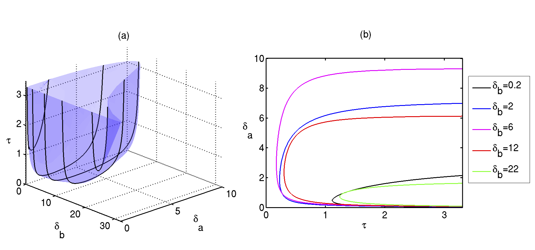
Figure 1: Stability boundary of the steady state $(\bar{p}_{a},\bar{p}_{b})$ of the DSNM system (8). The steady state is stable below the surface in (a) and to the left of the boundary curves shown in (b). Parameter values are $m_{a}=m_{b}=2.35$, $\theta_{a}=\theta_{b}=0.21$, $n_{a}=n_{b}=3$, and $k_{a}=k_{b}=\gamma_{a}=\gamma_{b}=1$.

Substituting the expressions for $\cos(\omega_{0}\tau_{0,n})$ and $\sin(\omega_{0}\tau_{0,n})$ from the system (11) gives

$$\mbox{sgn}\left\{\left[\frac{d(Re\lambda)}{d\tau}\right]_{\tau=\tau_{0,n}}\right\}=\mbox{sgn}\left\{\frac{2(\omega_{0}^{2}-\delta_{a}\delta_{b})+(\delta_{a}+\delta_{b})^{2}}{D_{\text{DSNM}}^{2}}\right\}=\mbox{sgn}\left\{\frac{h^{\prime}(\omega_{0}^{2})}{D_{\text{DSNM}}^{2}}\right\}>0.$$

Hence, the eigenvalues of the characteristic equation cross the imaginary axis at $\tau=\tau_{0}$ (here, $\tau_{0}=\tau_{0,0}$) and never cross back for higher values of $\tau$. Thus, we have proved the following result.

Theorem 1. If $\delta_{a}\delta_{b}\geq D_{\text{DSNM}}$, the steady state $(\bar{p}_{a},\bar{p}_{b})$ of the DSNM system (8) is stable for all values of the time delay $\tau\geq 0$. If $\delta_{a}\delta_{b}<D_{\text{DSNM}}$, this steady state is stable for $0\leq\tau<\tau_{0}$, unstable for $\tau>\tau_{0}$, and undergoes a Hopf bifurcation at $\tau=\tau_{0}$.

Figure 1 illustrates the stability boundary of the steady state $(\bar{p}_{a},\bar{p}_{b})$ of the DSNM system (8) depending on the time delay $\tau$ and the protein degradation rates $\delta_{a}$ and $\delta_{b}$, with the parameter values taken from Polynikis et al. [44]. This Figure suggests that for any fixed value of one of such rates, there is only a limited range of positive values of the other degradation rate, for which at a given time delay $\tau$, the positive equilibrium is unstable. For sufficiently high values of $\delta_{a}$ and $\delta_{b}$, this steady state is stable regardless of the value of the time delay $\tau$, confirming the result proved in Theorem 1.

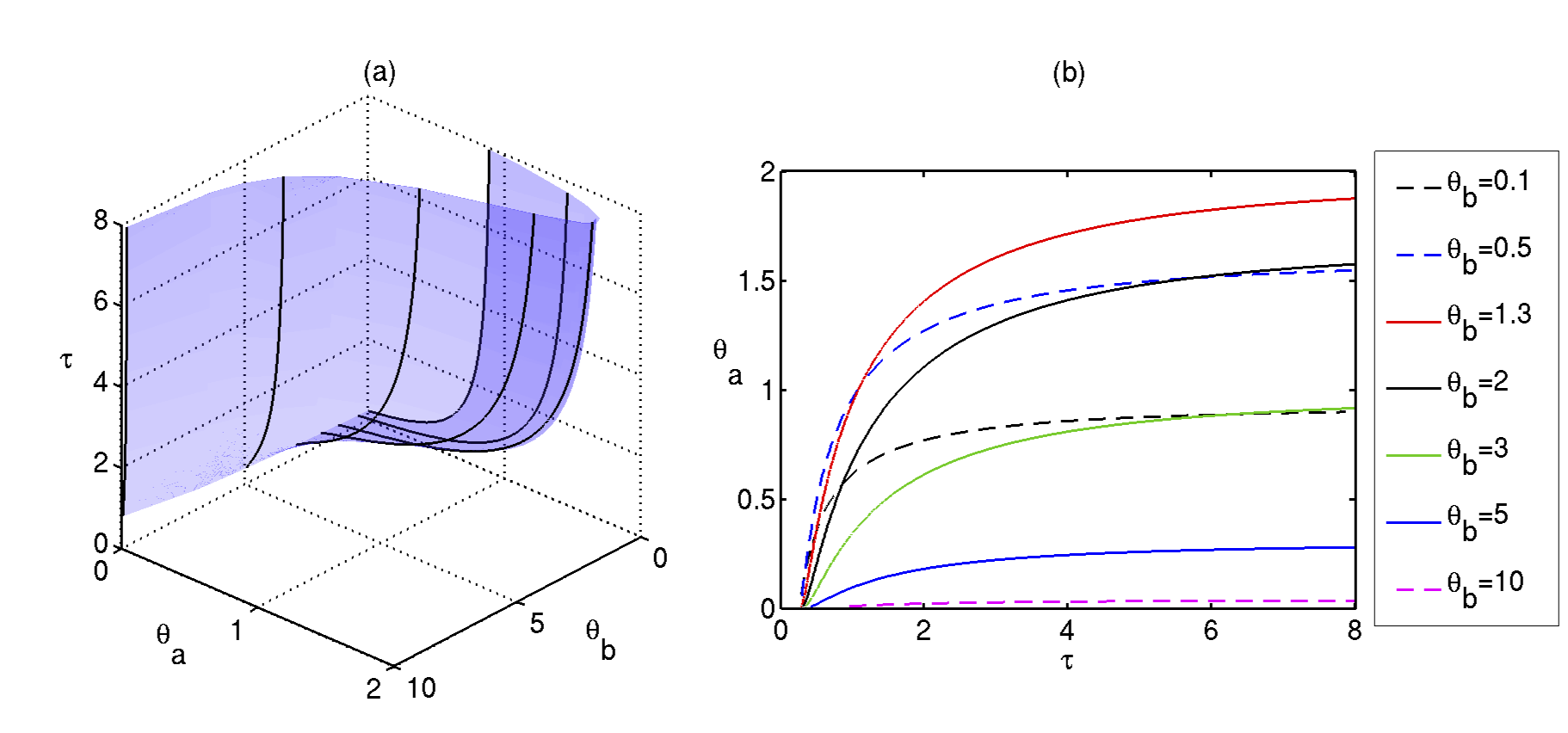
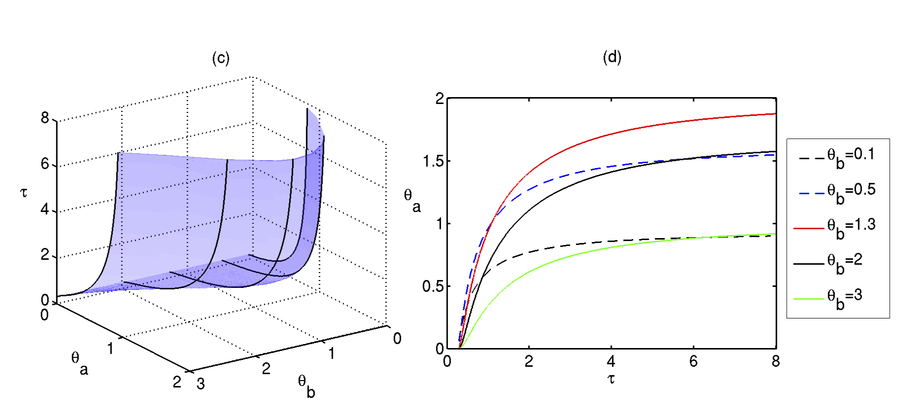
Figure 2: Stability boundary of the steady state $(\bar{p}_{a},\bar{p}_{b})$ of the DSNM system (8). The steady state is stable below the surface in (a), and to the left of the boundary curves shown in (b). Parameter values are $m_{a}=m_{b}=2.35$, $n_{a}=n_{b}=3$, and $k_{a}=k_{b}=\delta_{a}=\delta_{b}=\gamma_{a}=\gamma_{b}=1$.

In Fig. 2 we show how the stability boundary varies depending on the parameters $\theta_{a}$, $\theta_{b}$, and the time delay $\tau$. One observes that for sufficiently high values of the $\theta_{b}$, the range of possible values of $\theta_{a}$ for which the steady state is unstable is significantly reduced, thus making the system more prone to support a stable positive equilibrium rather that exhibit oscillations. At the Hopf bifurcation, the associated critical value of the time delay $\tau$ monotonically increases with the parameter $\theta_{a}$. At the same time, there is a minimum value of the time delay $\tau$, such that for $\tau$ smaller than this value the steady state $(\bar{p}_{a},\bar{p}_{b})$ is stable for any value of $\theta_{a}$.

In a similar way, the effects of the transcription rates $m_{a}$ and $m_{b}$ are illustrated in Fig. 3, which shows that the critical transcription rate of the inhibitor $m_{a}$ increases with decreasing $\tau$, and similar to Fig. 2, below certain value of $\tau$, the steady state $(\bar{p}_{a},\bar{p}_{b})$ is stable for any value of $m_{a}$. Qualitatively similar dependence is observed between the critical value of $\tau$ and the transcription rate $m_{b}$, though this dependence is not completely monotonic.

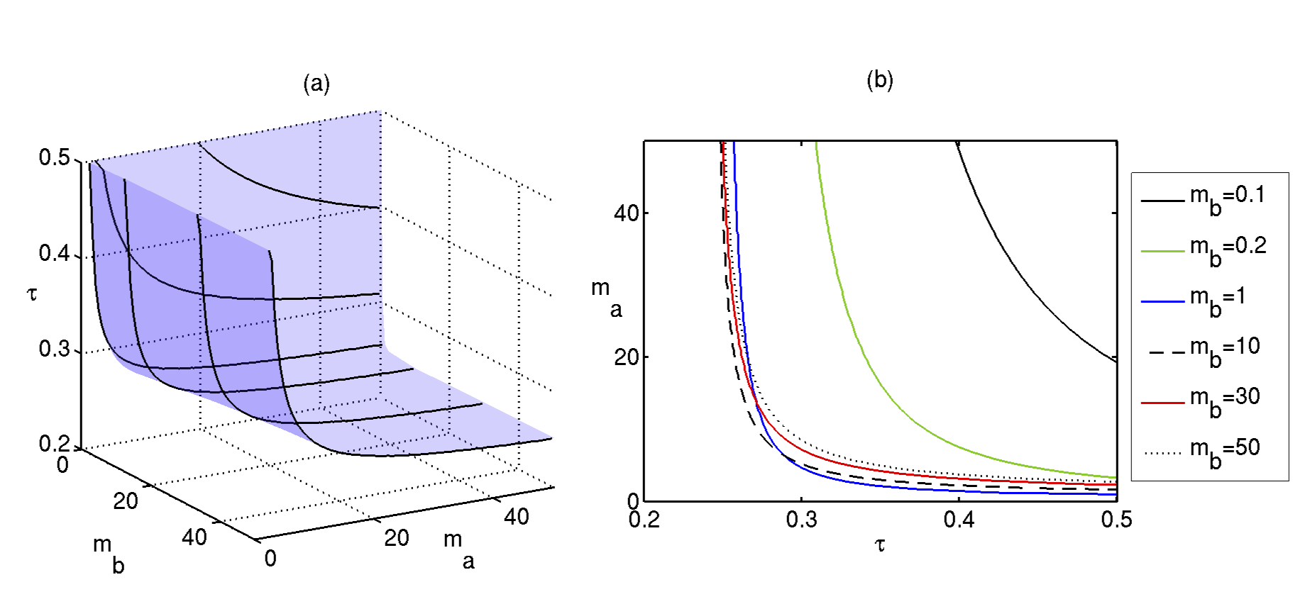
Figure 3: Stability boundary of the steady state $(\bar{p}_{a},\bar{p}_{b})$ of the DSNM system (8). The steady state is stable below the surface in (a), (c), and to the left of the boundary curves shown in (b), (d). Parameter values are $\theta_{a}=\theta_{b}=0.21$, $n_{a}=n_{b}=3$, and $k_{a}=k_{b}=\delta_{a}=\delta_{b}=\gamma_{a}=\gamma_{b}=1$.

Figure 4 demonstrates how increasing the overall time delay $\tau$ results in a Hopf bifurcation of the steady state $(\bar{p}_{a},\bar{p}_{b})$ and the emergence of a stable periodic orbit. The shift between individual time series for $p_{a}$ and $p_{b}$ can be interpreted in the same way as in predator-prey or activator-inhibitor systems [105]. In accordance with Theorem 1, once the stability of the steady state $(\bar{p}_{a},\bar{p}_{b})$ is lost, it can never be regained for higher values of $\tau$, so the system will be exhibiting oscillatory behaviour. This result highlights the significance of correct mathematical representation of the transcription and translation processes, since inclusion of transcriptional and translational delays can lead to sustained periodic oscillations even in the simplified model, where such oscillations were impossible when the time delays were neglected.

5 Analysis of the delayed complete non-linear model (DCNM)

Linearisation of the full nonlinear DCNM model (3) near the steady state $(\bar{r}_{a},\bar{r}_{b},\bar{p}_{a},\bar{p}_{b})$ results in the following characteristic equation

$$(\lambda+\gamma_{a})(\lambda+\gamma_{b})(\lambda+\delta_{a})(\lambda+\delta_{b})+D_{\text{DCNM}}e^{-\lambda\tau}=0,$$ (16)

where

$${D_{\text{DCNM}}=m_{a}m_{b}k_{a}k_{b}\theta_{a}^{n_{a}}\theta_{b}^{n_{b}}\frac{n_{a}n_{b}\bar{p}_{a}^{(n_{a}-1)}\bar{p}_{b}^{(n_{b}-1)}}{(\theta_{a}^{n_{a}}+\bar{p}_{a}^{n_{a}})^{2}(\theta_{b}^{n_{b}}+\bar{p}_{b}^{n_{b}})^{2}}=n_{a}n_{b}\delta_{a}\delta_{b}\frac{\bar{p}^{n_{a}}_{a}}{\theta^{n_{a}}_{a}+\bar{p}^{n_{a}}_{a}}\frac{\theta^{n_{b}}_{b}}{\theta^{n_{b}}_{b}+\bar{p}^{n_{b}}_{b}},}$$

and

$$\tau=\tau_{r_{a}}+\tau_{r_{b}}+\tau_{p_{a}}+\tau_{p_{b}}.$$

It immediately follows from the form of the characteristic equation (16) that stability of the steady state $(\bar{r}_{a},\bar{r}_{b},\bar{p}_{a},\bar{p}_{b})$ is determined not by individual transcriptional and translational delays, but rather by their overall combined duration. In the case $\tau_{r_{a}}=\tau_{r_{b}}=\tau_{p_{a}}=\tau_{p_{b}}=0$, the characteristic equation of the DCNM model reduces to the one analysed in Polynikis et al. [44].

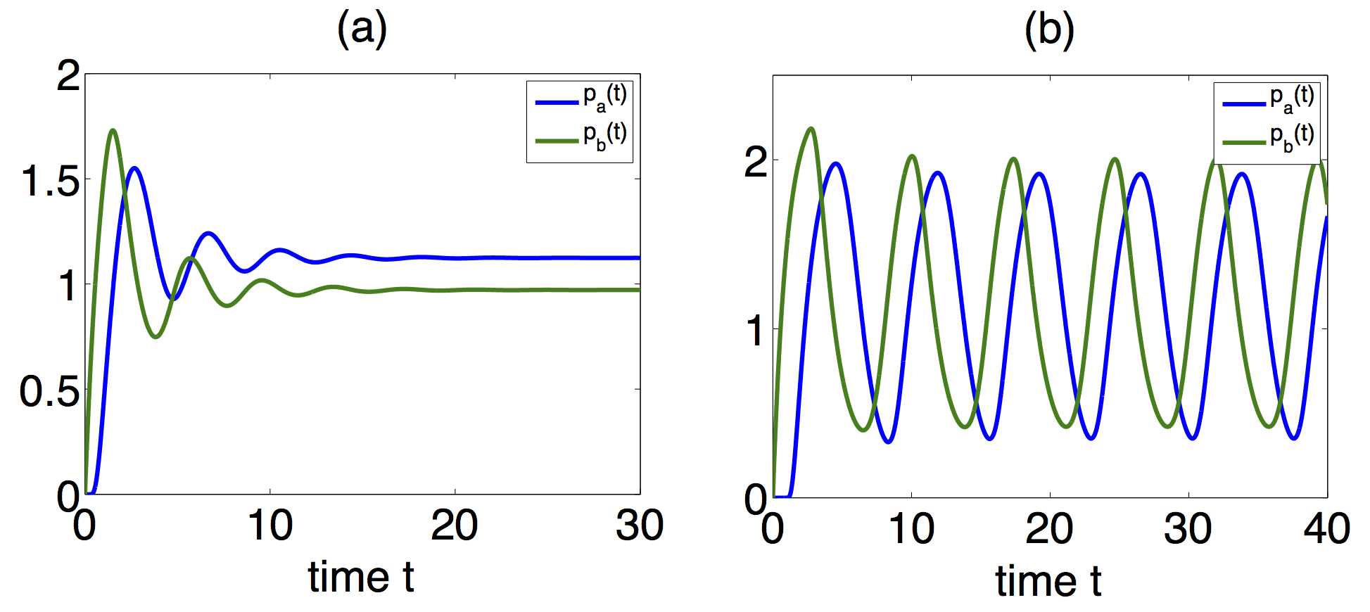
Figure 4: Numerical solution of the DSNM system (8). (a) $\tau=0.5$. (b) $\tau=2$. Parameter values are $m_{a}=m_{b}=2.35$, $\theta_{a}=\theta_{b}=1$, $n_{a}=n_{b}=3$, and $k_{a}=k_{b}=\delta_{a}=\delta_{b}=\gamma_{a}=\gamma_{b}=1$. The critical time delay is $\tau_{0}=0.9762$.

The characteristic equation (16) can be recast in the form

$$\lambda^{4}+A\lambda^{3}+B\lambda^{2}+C\lambda+(D+D_{\text{DCNM}}e^{-\lambda\tau})=0,$$ (17)

where,

$$\begin{array}[]{l}A=\gamma_{a}+\gamma_{b}+\delta_{a}+\delta_{b},\\ \\ B=\gamma_{a}\gamma_{b}+\gamma_{a}\delta_{a}+\gamma_{a}\delta_{b}+\gamma_{b}\delta_{a}+\gamma_{b}\delta_{b}+\delta_{a}\delta_{b},\\ \\ C=\gamma_{a}\gamma_{b}\delta_{a}+\gamma_{a}\gamma_{b}\delta_{b}+\gamma_{a}\delta_{a}\delta_{b}+\gamma_{b}\delta_{a}\delta_{b},\\ \\ D=\gamma_{a}\gamma_{b}\delta_{a}\delta_{b}.\end{array}$$ (18)

At $\tau=0$, equation (17) reduces to a quartic

$$\lambda^{4}+A\lambda^{3}+B\lambda^{2}+C\lambda+(D+D_{\text{DCNM}})=0.$$ (19)

By the Routh-Hurwitz criterion [105], the necessary and sufficient conditions for all roots of the equation (19) to have negative real parts are given by:

$$\begin{array}[]{l}\Delta_{1}=A>0,\\ \\ \Delta_{2}=AB-C>0,\\ \\ \Delta_{3}=ABC-A^{2}(D+D_{\text{DCNM}})>0,\\ \\ \Delta_{4}=(D+D_{\text{DCNM}})(ABC-A^{2}(D+D_{\text{DCNM}})-C^{2})=(D+D_{\text{DCNM}})(\Delta_{3}-C^{2})>0.\end{array}$$

From the fact that all system parameters are positive, and using the definitions of $A$, $B$ and $C$ in (18), it follows that $\Delta_{1}>0$ and $\Delta_{2}>0$ for any values of the parameters. Since $D+D_{\text{DCNM}}>0$, it is sufficient to require $\Delta_{4}>0$ to ensure that the condition $\Delta_{3}>0$ is also satisfied. This leads to the following result.

Lemma 1. Let $\tau=0$. The steady state $(\bar{r}_{a},\bar{r}_{b},\bar{p}_{a},\bar{p}_{b})$ of the system (3) is stable whenever the condition $ABC-A^{2}(D+D_{\textnormal{DCNM}})-C^{2}>0$ holds.

From now on, we will assume that the condition in Lemma 1 holds, and analyse whether stability can be lost as $\tau$ increases. Since both $D$ and $D_{\text{DCNM}}$ are positive, this means that $\lambda=0$ is not a root of the characteristic equation (17), so once again the stability can only be lost through a possible Hopf bifurcation. To investigate this possibility, we look for solutions of the equation (17) in the form $\lambda=i\omega$ for some real $\omega>0$. Substituting this into the equation (17) and separating into the real and imaginary parts gives

$$\begin{array}[]{l}\omega^{4}-B\omega^{2}+D=-D_{\text{DCNM}}\cos(\omega\tau),\\ \\ -A\omega^{3}+C\omega=D_{\text{DCNM}}\sin(\omega\tau).\end{array}$$ (20)

Squaring and adding these equations yields a quartic equation

$$g(z)=z^{4}+az^{3}+bz^{2}+cz+d=0,$$ (21)

where $z=\omega^{2}$, and

$$\begin{array}[]{l}a=A^{2}-2B,\hskip 14.22636ptb=B^{2}+2D-2AC,\\ \\ c=C^{2}-2BD,\hskip 14.22636ptd=D^{2}-D_{\text{DCNM}}^{2}.\end{array}$$

Without the loss of generality, suppose that the equation (21) has four positive real roots, denoted by $z_{1},z_{2},z_{3},z_{4}$, respectively, which would give four possible values of $\omega$,

$$\omega_{1}=\sqrt{z_{1}},\hskip 5.69054pt\omega_{2}=\sqrt{z_{2}},\hskip 5.69054pt\omega_{3}=\sqrt{z_{3}},\hskip 5.69054pt\omega_{4}=\sqrt{z_{4}}.$$

Dividing the two equations in (20) gives

$$\tan(\omega_{k}\tau_{k})=\frac{A\omega_{k}^{3}-C\omega_{k}}{\omega_{k}^{4}-B\omega_{k}^{2}+D}\hskip 5.69046pt\Longrightarrow\hskip 5.69046pt\tau_{k,j}=\frac{1}{\omega_{k}}\left[\mbox{Arctan}\frac{A\omega_{k}^{3}-C\omega_{k}}{\omega_{k}^{4}-B\omega_{k}^{2}+D}+j\pi\right],\hskip 5.69046ptk=1,..,4,\hskip 5.69046ptj=0,1,2,...$$ (22)

Define

$$\tau_{0}=\min\limits_{1\leq k\leq 4}\{\tau_{k,0}\},\hskip 14.22636pt\omega_{0}=\omega_{k_{0}},\hskip 14.22636ptk_{0}\in\{1,2,3,4\},$$

then $\tau_{0}$ is the first value of $\tau>0$ such that the characteristic equation (17) has a pair of purely imaginary roots. We have the following result.

Theorem 2. Suppose the conditions of Lemma 1 hold, and $g^{\prime}(z_{0})>0$, where $g(z)$ is defined in Eq. (21). Then the steady state $(\bar{r}_{a},\bar{r}_{b},\bar{p}_{a},\bar{p}_{b})$ of the system (3) is stable for $0\leq\tau<\tau_{0}$, unstable for $\tau>\tau_{0}$, and undergoes a Hopf bifurcation at $\tau=\tau_{0}$.

Proof. The conclusion of Lemma 1 ensures the steady state $(\bar{r}_{a},\bar{r}_{b},\bar{p}_{a},\bar{p}_{b})$ of the system (3) is stable at $\tau=0$, and the fact that the roots of the characteristic equation (17) depend continuously on $\tau$ implies that the steady state $(\bar{r}_{a},\bar{r}_{b},\bar{p}_{a},\bar{p}_{b})$ is also stable for sufficiently small positive values of $\tau$. Since $\tau_{0}$ is the first positive $\tau$, for which the characteristic eigenvalues lie on the imaginary axis, in order to verify whether or not the steady state actually loses stability at $\tau=\tau_{0}$, one has to compute the sign of $dRe(\lambda)/d\tau|_{\tau=\tau_{0}}$. Let $\lambda(\tau)=\mu(\tau)+i\omega(\tau)$ be the root of the characteristic equation (17) near $\tau=\tau_{0}$, satisfying $\mu(\tau_{0})=0$, $\omega(\tau_{0})=\omega_{0}$. Substituting $\lambda=\lambda(\tau)$ into the Eq. (17) and differentiating both sides with respect to $\tau$ gives

$$\left(\frac{d\lambda}{d\tau}\right)^{-1}=\frac{(4\lambda^{3}+3A\lambda^{2}+2B\lambda+C)e^{\lambda\tau}}{\lambda D_{\text{DCNM}}}-\frac{\tau}{\lambda}.$$

This implies, with $\lambda(\tau_{0})=i\omega_{0}$,

$$\begin{array}[]{l}\displaystyle{\mbox{sgn}\left\{\left[\frac{d(Re\lambda)}{d\tau}\right]_{\tau=\tau_{0}}\right\}=\mbox{sgn}\left\{Re\left[\left(\frac{d\lambda}{d\tau}\right)^{-1}\right]_{\tau=\tau_{0}}\right\}=\mbox{sgn}\left\{Re\left[\frac{(4\lambda^{3}+3A\lambda^{2}+2B\lambda+C)e^{\lambda\tau}}{\lambda D_{\text{DCNM}}}\right]_{\tau=\tau_{0}}\right\}}\\ \\ \displaystyle{=\mbox{sgn}\left\{\frac{(2B\omega_{0}-4\omega_{0}^{3})\cos(\omega_{0}\tau_{0})+(C-3A\omega_{0}^{2})\sin(\omega_{0}\tau_{0})}{\omega_{0}D_{\text{DCNM}}}\right\}.}\end{array}$$

Using the expressions for $\cos(\omega_{0}\tau_{0})$ and $\sin(\omega_{0}\tau_{0})$ from Eq. (20) gives

$$\begin{array}[]{l}\displaystyle{\mbox{sgn}\left\{\left[\frac{d(Re\lambda)}{d\tau}\right]_{\tau=\tau_{0}}\right\}=\mbox{sgn}\left\{\frac{4\omega_{0}^{6}+(3A^{2}-6B)\omega_{0}^{4}+(2B^{2}+4D-4AC)\omega_{0}^{2}+C^{2}-2BD}{D_{\text{DCNM}}^{2}}\right\}}\\ \\ \displaystyle{=\mbox{sgn}\left\{\frac{g^{\prime}(\omega_{0}^{2})}{D_{\text{DCNM}}^{2}}\right\}>0,}\end{array}$$

which means that at $\tau=\tau_{0}$ a pair of complex conjugate eigenvalues of the characteristic equation (17) crosses the imaginary axis with a positive speed. This implies that the steady state $(\bar{r}_{a},\bar{r}_{b},\bar{p}_{a},\bar{p}_{b})$ of the system (3) does lose its stability at $\tau=\tau_{0}$. $\hfill\square$

Figure 5 shows the stability boundary of the steady state $(\bar{r}_{a},\bar{r}_{b},\bar{p}_{a},\bar{p}_{b})$ of the system (3) depending on the transcription rates $m_{a}$ and $m_{b}$, and the total time delay $\tau$. In a manner similar to that for the simplified model, the critical value of the transcription rate $m_{a}$ at the Hopf bifurcation reduces with increasing $\tau$. However, a major difference from the DSNM model, as shown in Fig. 3, is that now the Hopf bifurcation can take place even at $\tau=0$, as the DCNM system is able to support sustained oscillations [44].

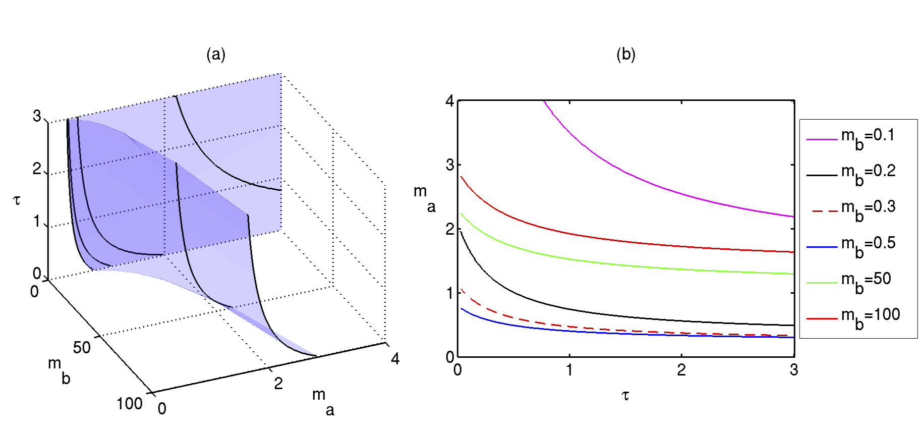
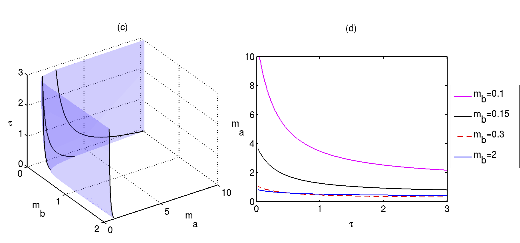
Figure 5: Stability boundary of the steady state $(\bar{r}_{a},\bar{r}_{b},\bar{p}_{a},\bar{p}_{b})$ of the DCNM system (3). The steady state is stable below the surface in (a), (c), and below the boundary curves shown in (b), (d). Parameter values: $\theta_{a}=\theta_{b}=0.21$, $n_{a}=n_{b}=3$ and $k_{a}=k_{b}=\delta_{a}=\delta_{b}=\gamma_{a}=\gamma_{b}=1$.

In Fig. 6 we illustrate the transition from a stable steady state $(\bar{r}_{a},\bar{r}_{b},\bar{p}_{a},\bar{p}_{b})$ to a stable periodic solution around this steady state as the time delay passes through the critical value of $\tau=\tau_{0}$.

6 Conclusions

In this review we have discussed various mathematical models for the analysis of GRNs, and focussed on the role played by the transcriptional and translational time delays in the dynamics of a two-gene activator-inhibitor GRN. By reducing the model to the one with a single time delay, we have considered possible behaviour in the quasi-steady state approximation of very fast mRNA dynamics, which has resulted in a lower-dimensional system of DDEs. Due to the presence of time delays, even this simplified model is able to exhibit loss of stability of the positive equilibrium through a Hopf bifurcation, and a subsequent emergence of sustained periodic oscillations, which was not possible in the absence of the time delays, as discussed in Polynikis et al. [44]. We have found analytically the boundary of the Hopf bifurcation depending on the total time delay and other system parameters, and illustrated different types of behaviour by direct numerical simulations. Our results suggest that once the positive steady state loses its stability, it can never regain it for higher values of the time delay.

We have also studied the stability of a positive steady state in the full system and showed that this steady state can also undergo a Hopf bifurcation depending on the time delay and system parameters. Our analysis extends an earlier result of Polynikis et al. [44] by showing how the critical values of the parameters at the Hopf boundary change when the time delay increases from zero. Numerical simulations have illustrated the transition from a stable positive steady state to a stable periodic solution as the time delay exceeds its critical value.

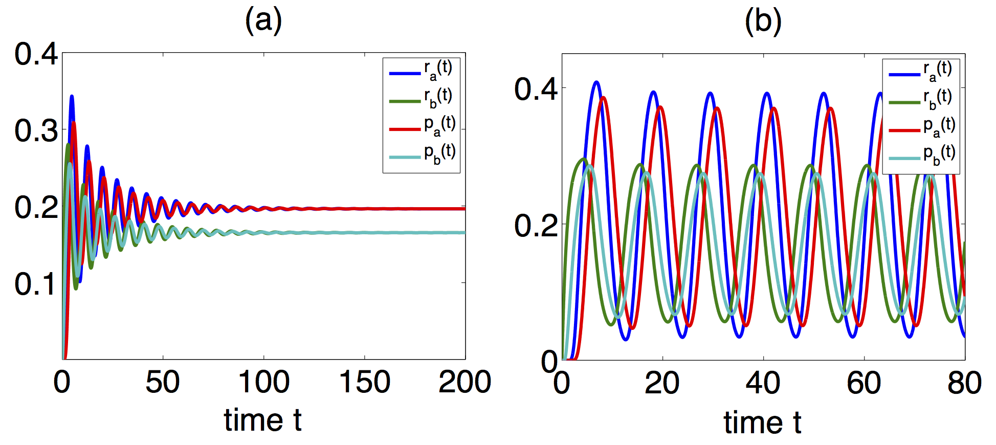
Figure 6: Numerical solution of the DCNM system (3). (a) $\tau=0.25$. (b) $\tau=2$. Parameter values: $m_{a}=0.6$, $m_{b}=0.3$, $\theta_{a}=\theta_{b}=0.21$, $n_{a}=n_{b}=3$, and $k_{a}=k_{b}=\delta_{a}=\delta_{b}=\gamma_{a}=\gamma_{b}=1$. The critical time delay is $\tau_{0}=0.5314$.

The work presented in the paper can be extended in several interesting and important research directions. One possibility would be to account for the fact that in most experiments the transcriptional and translational time delay are not fixed but rather obey some form of a delay distribution. Recent work on the effects on delay distribution on system dynamics [106, 107, 108] has shown that even for the same mean delay, details of the distribution can also play an important role. He and Cao [71] have used Lyapunov functional approach to derive conditions for global stability of equilibria in some types of GRNs with distributed delays, and it would be insightful to investigate the possibility of extending this methodology to other types of GRNs and various types of delay kernels. Alternatively, one could use the framework of a master stability function for systems with distributed delays [109] to study possible synchronization dynamics in GRNs with a large number of proteins involved.

As it has already been mentioned, in some cases gene expression behaviour is characterised by a switch-like behaviour that can be better modelled using piecewise-linear rather than continuous transcription functions [50, 53]. Whilst some preliminary work has been done recently on the analysis of piecewise-linear systems with discrete time delays, primarily in engineering applications [110, 111, 112], the dynamics of GRNs with piecewise-linear transcription functions and transcriptional/translational delays has remained completely unexplored. Further inclusion of distributed delays would make such models mathematically very challenging, but it could provide a new level of understanding of GRN dynamics.

Besides providing insights into the dynamics of GRNs, there are several practical ways in which models similar to the one described in this review are helpful for monitoring and treatment of cancer. GRN models based on differential equations coupled with other techniques, such as machine learning and Bayesian networks, have proved effective in identifying specific oncogenes that can be used as biomarkers or drug targets [62, 113, 114, 115, 116, 117]. Similar kinds of models are useful for modelling cancer cell growth, understanding interactions between tumour growth and immune response, and for analysis of the effects of chemotherapy (or immunotherapy) and drug resistance [62, 63, 118, 119]. The methodology described in this review can be directly used to improve the performance of these models by elucidating the role of transcriptional and translational time delays in GRN dynamics and its impact on various aspects of cancer onset and development.

Conflict of interest

The authors declare that there is no conflict of interests regarding the publication of this paper.

References

- [1] G. Danaei, S. Vander Hoorn, A.D Lopez, C.J.L. Murray, M. Ezzati, ”Causes of cancer in the world: comparative risk assessment of nine behavioural and environmental risk factors,” The Lancet, vol. 366, pp. 1784-1793, 2005.
- [2] M. Boshart, L. Gissmann, H. Ikenberg, A. Kleinheinz, W. Scheurlen, H. zur Hausen, ”A new type of papillomavirus DNA, its presence in genital cancer biopsies and in cell lines derived from cervical cancer,” The EMBO Journal, vol. 3, no. 5, pp. 1151-1157, 1984.
- [3] D.F. Easton, ”How many more breast cancer predisposition genes are there?” Breast Cancer Research, vol. 1, no. 1, pp. 14-17, 1999.
- [4] G. Thomas, K.B. Jacobs, M. Yeager, P. Kraft, S. Wacholder et al., ”Multiple loci identified in a genome-wide association study of prostate cancer”, Nature Genetics, vol. 40, no. 3, pp. 310-315, 2008.
- [5] B.M. Wolpin, C. Rizzato, P. Kraft, C. Kooperberg, G.M. Petersen et al., ”Genome-wide association study identifies multiple susceptibility loci for pancreatic cancer,” Nature Genetics, vol. 46, no. 9, pp. 994-1000, 2014.
- [6] U. Alon, An introduction to systems biology, Champan & Hall, Boca Raton, USA, 2007.
- [7] H. de Jong, ”Modeling and simulation of genetic regulatory systems: a literature review”, Journal of Computational Biology, vol. 9, no. 1, pp. 67-103 (2002).
- [8] G. Bernot, J.-P. Comet, A. Richard, M. Chaves, J.-L. Gouzé, R. Dayan, ”Modeling and analysis of gene regulatory networks”, pp. 47-80, in F. Cazals, P. Kornprobst (Eds.), Modeling in Computational Biology and Biomedicine, Springer Verlag, Berlin, 2013.
- [9] H.-Y. Yeh, S.-W. Cheng, Y.-C. Lin, C.-Y. Yeh, S.-F. Lin, V.-W. Soo, ”Identifying significant genetic regulatory networks in the prostate cancer from microarray data based on transcription factor analysis and conditional independency,” BMC Medical Genomics vol. 2, Article ID 70, 2009.
- [10] E. Bonnet, T. Michoel, Y. Van de Peer, ”Prediction of a gene regulatory network linked to prostate cancer from gene expression, microRNA and clinical data,” Bioinformatics, vol. 26, no. 18, pp. i638-i644, 2010.
- [11] X. Wang, O. Gotoh, ”Inference of cancer-specific gene regulatory networks using soft computing rules,” Gene Regulation and Systems Biology, vol. 4, pp. 19-34, 2010.
- [12] S. Vineetha, C. Chandra Shekara Bhat, S.M. Idicula, ”Gene regulatory network from microarray data of colon cancer patients using TSK-type recurrent neural fuzzy network,” Gene, vol. 506, no. 2, pp. 408-416, 2012.
- [13] P.B. Madhamshettiwar, S.R. Maetschke, M.J. Davis, A. Reverter, M.A. Ragan, ”Gene regulatory network inference: evaluation and application to ovarian cancer allows the prioritization of drug targets,” Genome Medicine, vol. 4, Article ID 41, 2012.
- [14] F.K. Ahmad, S. Deris, N.H. Othman, ”The inference of breast cancer metastasis through gene regulatory networks,” Journal of Biomedical Informatics, vol. 45, no. 2, pp. 350-362, 2012.
- [15] F. Emmert-Streib, R. de Matos Simoes, P. Mullan, B. Haibe-Kains, M. Dehmer, ”The gene regulatory network for breast cancer: integrated regulatory landscape of cancer hallmarks,” Frontiers in Genetics, vol. 5, Article 15, 2014.
- [16] D. Endy, R. Brent, ”Modelling cellular behaviour,” Nature, vol. 409, pp. 391-395, 2001.
- [17] J. Hasty, D. McMillen, F. Isaacs, J.J. Collins, ”Computational studies of gene regulatory networks: in numero molecular biology,” Nature Reviews Genetics, vol. .2, pp. 268-279, 2001.
- [18] A. Tušek, Z. Kurtanjek, ”Mathematical Modelling of Gene Regulatory Networks,” Intechopen, 2012.
- [19] M. Hecker, S. Lambeck, S. Toepfer, E. van Someren, R. Guthke, ”Gene regulatory network inference: Data integration in dynamic models - A review,” BioSystems, vol.69, no.1, pp. 86-103, 2009.
- [20] S.A.Kauffman, ”Metabolic stability and epigenesis in randomly constructed genetic nets,” Journal of Theoretical Biology, vol. 22, pp. 437-467, 1969.
- [21] R. Thomas, Boolean formalization of genetic control circuits. Journal of Theoretical Biology, vol. 42, pp. 563-585, 1973.
- [22] R. Somogyi, C.A. Sniegoski, ”Modeling the complexity of genetic networks: Understanding multigenic and pleiotropic regulation,” Complexity, vol. 1, no. 6, pp. 45-63, 1996.
- [23] R. Albert, ”Boolean modelling of genetic regulatory networks”, Lecture Notes in Physics, vol. 650, pp. 459-481, 2004.
- [24] P. Smolen, D.A. Baxter, J.H. Byrne, ”Modeling transcriptional control in gene networks methods, recent results, and future directions,” Bulletin of Mathematical Biology, vol. 62, no. 2, pp. 247-292, 2000.
- [25] I. Shmulevich, E.R. Dougherty, W. Zhang, ”From Boolean to probabilistic Boolean networks and models of genetic regulatory networks,” Proceedings of the IEEE, vol. 90, no. 11, pp. 1778-1792, 2002.
- [26] A. Silvescu, V. Honavar, ”Temporal Boolean network models of genetic networks and their Inference from gene expression time series,” Complex Systems, vol. 13, pp. 61-78, 2001.
- [27] M. Davidich, S. Bornholdt, ”The transition from differential equations to Boolean networks: A case study,” Journal of Theoretical Biology, vol. 255, no. 3, pp. 269-277, 2008.
- [28] R. Xu, G.K. Venayagamoorthy, D.C. Wunsch, ”Modelling of gene regulatory networks with hybrid differential evolution and particle swarm optimization,” Neural Networks, vol. 20, pp. 917-927, 2007.
- [29] F. Karlsson, M. Hörnquist, ”Order or chaos in Boolean gene networks depends on the mean fraction of canalizing functions,” Physica A, vol. 384, no. 2, pp. 747-757, 2007.
- [30] G. N. Brock, V. Pihur, and L. Kubatko, Detecting gene regulatory networks from microarray data using fuzzy logic, pp. 141-163, in Y. Jin and L. Wang (Eds.), Fuzzy Systems in Bioinformatics and Computational Biology, vol. 242 of Studies in Fuzziness and Soft Computing, Springer, Berlin,Germany, 2009.
- [31] P.J. Woolf and Y. Wang, A fuzzy logic approach to analyzing gene expression data, Physiological Genomics, vol. 3, no. 1, pp. 9-15, 2000.
- [32] L.G. Volkert and N. Malhis, An efficient method for fuzzy identification of regulatory events in gene expression time series data, in Proceedings of the IEEE Symposium on Computational Intelligence in Bioinformatics and Computational Biology (CIBCB 04), pp. 17-24, October 2004.
- [33] P. Das, P. Rakshit, A. Konar, M. Nasipuri, and A. K. Nagar, Fuzzy relational system for identification of gene regulatory network, in Proceedings of the WorldComp, 2009.
- [34] T.A. Al Qazlan, A. Hamdi-Cherif, C. Kara-Mohamed, ”State of the art of fuzzy methods for gene regulatory networks inference,” The Scientific World Journal, vol. 2015, Article ID 148010, 2015.
- [35] B.C. Goodwin, Temporal Organization in Cells, Academic Press, New York, 1963.
- [36] B.C. Goodwin, ”Oscillatory behavior in enzymatic control processes”, in G. Weber (Ed.), Advances in enzyme regulation, pp. 425-438, Pergamon Press, Oxford, 1965.
- [37] J.-L. Gouzé, ”Positive and negative circuits in dynamical systems,” Journal of Biological Systems vol. 6, no. 1, pp. 11-15, 1998.
- [38] E.H. Snoussi, ”Necessary conditions for multistationarity and stable periodicity,” Journal of Biological Systems, vol. 6, no. 1, pp. 3-9, 1998.
- [39] J.J. Tyson, H.G. Othmer, ”The dynamics of feedback control circuits in biochemical pathways,” Progress in Theoretical Biology, vol. 5, pp. 1-62, 1975.
- [40] A.D. Keller, ”Specifying epigenetic states with autoregulatory transcription factors”, Journal of Theoretical Biology, vol. 170, 175-181, 1994.
- [41] R. Heinrich, S. Schuster, The Regulation of Cellular Systems, Chapman and Hall, New York, 1996.
- [42] J.L. Cherry, F.R. Adler, ”How to make a biological switch,” Journal of Theoretical Biology, vol. 203, pp. 117-133, 2000.
- [43] G. Yagil, ”Quantitative aspects of protein induction,” Current Topics in Cell Regulations, vol. 9, pp. 183-235, 1975.
- [44] A. Polynikis, S.J. Hogan, M. di Bernado, ”Comparing different ODE modelling approaches for gene regulatory networks,” Journal of Theoretical Biology, vol. 261, no. 4, pp. 511-530, 2009.
- [45] S. Widder, J. Schicho, P. Schuster, ”Dynamic patterns of gene regulation I: simple two-gene systems,” Journal of Theoretical Biology, vol. 246, no. 3, pp. 395-419, 2007.
- [46] S. Goutelle, M. Maurin, F. Rougier, X. Barbaut, L. Bouguignon, M. Ducher, P. Maire, ”The Hill equation: a review of its capabilities in pharmacological modelling,” Fundamental and Clinical Pharmacology, vol. 22, pp. 633 648, 2008.
- [47] J.N. Weiss, ”The Hill equation revisited: uses and misuses,” The Journal of the Federation of American Societies for Experimental Biology, vol. 11, no. 11, pp. 835-841, 1997.
- [48] M. Santillán, ”On the use of the Hill functions in mathematical models of gene regulatory networks,” Mathematical Modelling of Natural Phenomena, vol. 3, no. 2, pp. 85-97, 2008.
- [49] L. Glass, S.A. Kauffman, ”The logical analysis of continuous non-linear biochemical control networks,” Journal of Theoretical Biology, vol. 39, no. 1, pp. 103-129, 1973.
- [50] L. Glass, ”Classification of biological networks by their qualitative dynamics,” Journal of Theoretical Biology, vol. 54, no. 1, pp. 85-107, 1975.
- [51] E. Plahte, T. Mestl, , S.W. Omholt, ”A methodological basis for description and analysis of systems with complex switch-like interactions,” Journal of Mathematical Biology, vol. 36, pp. 321-348, 1998.
- [52] E. Plahte, S. Kjøglum, ”Analysis and generic properties of gene regulatory networks with graded response functions,” Physica D, vol. 201, pp. 150-176, 2005.
- [53] R. Casey, H. de Jong, J.-L. Gouzé, ”Piecewise-linear models of genetic regulatory networks: equilibria and their stability,” Journal of Mathematical Biology, vol. 52, no. 1, pp. 27-56, 2006.
- [54] J. Gebert, N. Radde, G.-W. Weber, ”Modeling gene regulatory networks with piecewise linear differential equations,” European Journal of Operational Research, vol. 181, no. 3, pp. 1148-1165, 2007.
- [55] E. Plahte, T. Mestl, S.W. Omholt, ”Global analysis of steady points for systems of differential equations with sigmoid interactions,” Dynamics and Stability of Systems, vol. 9, no. 4, pp. 275-291, 1994.
- [56] E.H. Snoussi, R. Thomas, ”Logical identification of all steady states: The concept of feedback loop characteristic states,” Bulletin of Mathematical Biology, vol. 55, no. 5, pp. 973-991, 1993.
- [57] A. Hoffmann, A. Levchenko, M.L. Scott, D. Baltimore, ”The IB-NFB signaling module: temporal control and selective gene activation, Science, vol. 298, no. 5596, pp. 1241-1245, 2002.
- [58] S.L. Werner, D. Barken, A. Hoffmann, ”Stimulus specificity of gene expression programs determined by temporal control of IKK activity,” Science, vol. 309, no. 5742, pp. 1857-1861, 2005.
- [59] N. Geva-Zatorsky, N. Rosenfeld, S. Itzkovitz, R. Milo, A. Sigal, E. Dekel, T. Yarnitzky, Y. Liron, P. Polak, G. Lahav, U. Alon, ”Oscillations and variability in the p53 system,” Molecular Systems Biology, vol. 2, no. 1, pp. 2006.0033, 2006.
- [60] L. Ma, J. Wagner, J.J. Rice, W. Hu, A.J. Levine, G.A. Stolovitzky, ”A plausible model for the digital response of p53 to DNA damage,” Proceedings of the National Academy of Sciences of the United States of America, vol. 102, no. 40, pp. 14266-14271, 2005.
- [61] B.T. Hennessy, D.L. Smith, P.T. Ram, Y. Lu, G.B. Mills, ”Exploiting the PI3K/AKT pathway for cancer drug discovery,” Nature Reviews Drug Discovery, vol. 4, no. 12, pp. 988-1004, 2005.
- [62] T.M.K. Cheng, S. Gulati, R. Agius, P.A. Bates, ”Understanding cancer mechanisms through network dynamics,” Briefings in Functional Genomics, vol. 11, no. 6, pp. 543-560, 2012.
- [63] L.B. Edelman, J.A. Eddy, N.D. Price, ”In silico models of cancer,” Wiley Interdiscip Rev Syst Biol Med., vol. 2, no.4, pp. 438-459, 2010.
- [64] N. Monk, ”Oscillatory expression of Hes1, p53, and NF-B driven by transcriptional time delays,” Current Biology, vol. 13, no. 16, pp. 1409-1413, 2003.
- [65] A. Wan, X. Zou, ”Hopf bifurcation analysis for a model of genetic regulatory system with delay,” Journal of Mathematical Analysis and Applications, vol. 356, no. 2, pp. 464-476, 2009.
- [66] K. Wang, L. Wang, Z. Teng, H. Jiang, ”Stability and bifurcation of genetic regulatory networks with delays,” Neurocomputing, vol. 73, no. 16-18, pp. 2882-2892, 2010.
- [67] M. Bodnar, U. Foryś, J. Poleszczuk, ”Analysis of biochemical reactions models with delays,” Journal of Mathematical Analysis and Applications, vol. 376, no. 1, pp. 74-83, 2011.
- [68] Z. Wang, Z. Liu, R. Yuan, ”Stability and bifurcation in gene regulatory network model with delay,” Zeitschrift für Angewandte Mathematik und Mechanik, vol. 92, no. 4, pp. 290-303, 2012.
- [69] M. Xiao, W. Zheng, J. Cao, ”Stability and bifurcation of genetic regulatory networks with small RNAs and multiple delays,” International Journal of Computer Mathematics, vol. 91, no. 5, pp. 907-927, 2014.
- [70] M. Xiao, J. Cao, ”Genetic oscillation deduced from Hopf bifurcation in a genetic regulatory network with delays,” Mathematical Biosciences, vol. 215, no. 1, pp. 55-63, 2008.
- [71] W. He, J. Cao, ”Robust stability of genetic regulatory networks with distributed delay,” Cognitive Neurodynamics, vol. 2, no. 4, pp. 355-361, 2008.
- [72] B.D. Aguda, Y. Kim, M.G. Piper-Hunter, A. Friedman, C.B. Marsh, ”MicroRNA regulation of a cancer network: Consequences of the feedback loops involving miR-17-92, E2F, and Myc,” Proceedings of the National Academy of Sciences of the United States of America, vol. 105, no. 50, pp.19678-19683, 2008.
- [73] B.D. Aguda, ”Modeling microRNA-transcription factor networks in cancer,” pp. 149-167, in U. Schmitz, O. Wolkenhauer, J. Vera, ”MicroRNA cancer regulation: advanced concepts, bioinformatics and systems biology,” Springer Verlag, Dordrecht, 2013.
- [74] A.S. Ribeiro, J.J. Grefenstette, S.A. Kauffman, ”Modeling gene regulatory networks with delayed stochastic dynamics,”, pp. 198-218, in S. Das, D. Caragea, S.M. Welch, W.H. Hsu, ”Handbook of research on computational methodologies in gene regulatory networks”, Medical Information Science Reference, New York, 2010.
- [75] N. MacDonald, ”Time lag in a model of a biochemical reaction sequence with end product inhibition,” Journal of Theoretical Biology, vol. 67, no. 3, pp. 549-556, 1977.
- [76] I.R. Epstein, Y. Luo, ”?Differential delay equations in chemical kinetics. Nonlinear models: the cross-shaped phase diagram and the Oregonator,” Journal of Chemical Physics, vol. 95, no. 1, pp. 244-254, 1991.
- [77] J. Paulsson, ”Models of stochastic gene expression,” Physics of Life Reviews, vol. 2, no. 2, 2005.
- [78] S. Rosenfeld, ”Stochastic cooperativity in non-linear dynamics of gene regulatory networks,” Mathematical Biosciences, vol. 210, no. 1, pp. 121-142, 2007.
- [79] A. Raj, A. van Oudenaarden, ”Stochastic gene expression and its consequences,” Cell, vol. 135, no. 2, pp. 216-226, 2008.
- [80] P.S. Swain, M.B. Elowitz, E.D. Siggia, ”Intrinsic and extrinsic contributions to stochasticity in gene expression,” Proceedings of the National Academy of Sciences of the USA, vol. 99, no. 20, pp. 12795-12800, 2002.
- [81] K. Herbert, A. La Porta, B. Wong, R. Mooney, K. Neuman, R. Landick, S. Block, ”Sequence resolved detection of pausing by single RNA polymerase molecules,” Cell, vol. 125, pp. 1083-1094, 2006.
- [82] A.S. Ribeiro, O.-P. Smolander, T. Rajala, A. Hakkinen, O. Yli-Harja, ”Delayed stochastic model of transcription at the single nucleotide level,” Journal of Computational Biology, vol. 16, no. 4, pp. 539-553, 2009.
- [83] M. Voliotis, N. Cohen, C. Molina-Paris, T. Liverpool, ”Fluctuations, pauses and backtracking in DNA transcription,” Biophysical Journal, vol. 94, no. 2, pp. 334-348, 2008.
- [84] A.S. Ribeiro, ”Stochastic and delayed stochastic models of gene expression and regulation,” Mathematical Biosciences, vol. 223, pp. 1-11, 2010.
- [85] M. Dunlop, R. Cox, A. Levine, R. Murray, M. Elowitz, ”Regulatory activity revealed by dynamic correlations in gene expression noise,” Nature Genetics, vol. 40, no.12, pp. 1493-1498, 2008.
- [86] M.B. Elowitz, S. Leibler, ”A synthetic oscillatory network of transcriptional regulators,” Nature, vol. 403, no. 6767, pp. 335-338, 2000.
- [87] M.B. Elowitz, A.J. Levine, E.D. Siggia, P.S. Swain, ”Stochastic gene expression in a single cell,” Science, vol. 297, no. 5584, pp.1183-1186, 2002.
- [88] S. Rosenfeld, ”Stochastic oscillations in genetic regulatory networks: application to microarray experiments,” EURASIP Journal on Bioinformatics and Systems Biology, vol. 2006, Article ID 59526, 2006.
- [89] M. Kærn, T.C. Elston, W.J. Blake, J.J. Collins, ”Stochasticity in gene expression: from theories to phenotypes”, Nature Reviews Genetics, vol. 6, pp. 451-464, 2005.
- [90] D. Bratsun, D. Volfson, L.S. Tsimring, J. Hasty, ”Delay-induced stochastic oscillations in gene regulations,” Proceedings of the National Academy of Sciences of the United States of America, vol. 102, no. 41, pp. 14593-14598, 2005.
- [91] E. Zavala, T.T. Marquez-Lago, ”Delays induce novel stochastic effects in negative feedback gene circuits,” Biophysical Journal, vol. 106, pp. 467-478, 2014.
- [92] T.S. Gardner, C.R. Cantor, J.J. Collins, ”Construction of a genetic toggle switch in Escherichia coli,” Nature, vol. 403, no. 6767, pp. 339-342, 2000.
- [93] H. El Samad, M. Khammash, L. Petzold, D. Gillespie, ”Stochastic modelling of gene regulatory networks,” International Journal of Robust and Nonlinear Control, vol. 15, pp. 691-711, 2005.
- [94] M. Barrio, K. Burrage, A. Leier, T. Tian, ”Oscillatory regulation of Hes1: discrete stochastic delay modelling and simulation,” PLoS Computational Biology, vol. 2, no. 9, Article ID e117, 2006.
- [95] X. Cai, ”Exact stochastic simulation of coupled chemical reactions with delays,” Journal of Chemical Physics, vol. 127, Article ID 124108, 2007.
- [96] M. Jansen, P. Pfaffelhuber, ”Stochastic gene expression with delay,” Journal of Theoretical Biology, vol. 364, pp. 355-363, 2015.
- [97] N. Friedman, M. Linial, I. Nachman, D. Peer, ”Using Bayesian networks to analyze expression data,” Journal of Computational Biology, vol. 7, no. 6, pp. 601-620, 2000.
- [98] D. Heckerman, ”A tutorial on learning with Bayesian networks,” Microsoft Research Technical Report, MSR-TR-95-06, 1996.
- [99] A.V. Werhli, D. Husmeier, ”Reconstructing gene regulatory networks with Bayesian networks by combining expression data with multiple sources of prior knowledge,” Statistic Applied to Genetics and Molecular Biology, vol. 6, Article 15, 2007.
- [100] P.T. Spellman, G. Sherlock, M. Zhang, V. Iyer, K. Anders et al., ”Comprehensive identification of cell cycle-regulated genes of the yeast Saccharomyces cerevisiae by microarray hybridization,” Molecular Biology of the Cell, vol. 9, no. 12, pp. 3273-3297, 1998.
- [101] R.J. Prill, P.A. Iglesias, A. Levchenko, ”Dynamic properties of network motifs contribute to biological network organization,” PLoS Biology, vol. 3, no. 11, Article ID e343.
- [102] Y.N. Kyrychko, K.B. Blyuss, ”Global properties of a delayed SIR model with temporary immunity and nonlinear incidence rate,” Nonlinear Analysis Real World Applications, vol. 6, no. 3, pp. 495-507, 2005.
- [103] H.B. Tiedemann, E. Schneltzer, S. Zeiser et al., ”From dynamic expression patterns to boundary formation in the presomitic mesoderm,” PLoS Computational Biology, vol. 6, Article ID e1002586, 2012.
- [104] C. Li, J. Wang, ”Quantifying cell fate decisions for differentiation and reprogramming of a human stem cell network: landscape and biological paths,” PLoS Computational Biology, vol. 9, Article ID e1003165, 2013.
- [105] J.D. Murray, Mathematical biology: I. An Introduction, Springer Verlag, New York, USA, 2002.
- [106] K.B. Blyuss, Y.N. Kyrychko, ”Stability and bifurcations in an epidemic model with varying immunity period,” Bulletin of Mathematical Biology, vol. 72, no. 2, pp. 490-505, 2010.
- [107] Y.N. Kyrychko, K.B. Blyuss, E. Schöll, ”Amplitude death in systems of coupled oscillators with distributed-delay coupling,” European Physical Journal B, vol. 84, no. 2, pp. 307-315, 2011.
- [108] Y.N. Kyrychko, K.B. Blyuss, E. Schöll, ”Amplitude and phase dynamics in oscillators with distributed-delay coupling,” Philosophical Transactions of the Royal Society A, vol. 371, Article ID 20120466, 2013.
- [109] Y.N. Kyrychko, K.B. Blyuss, E. Schöll, ”Synchronization of networks of oscillators with distributed delay coupling,” Chaos, vol. 24, Article ID 043117, 2014.
- [110] M. Lakshmanan, D.V. Senthilkumar, Dynamics of nonlinear time-delay systems, Springer Verlag, Berlin, Germany, 2010.
- [111] R. Suresh, D. V. Senthilkumar, M. Lakshmanan, J. Kurths, ”Transition to complete synchronization and global intermittent synchronization in an array of time-delay systems,” Physical Review E, vol. 86, no. 1, Article ID 016212, 2012.
- [112] J. Sieber, P. Kowalczyk, S.J. Hogan, M. Di Bernardo, ”Dynamics of symmetric dynamical systems with delayed switching,” Journal of Vibration and Control, vol. 16, no. 7-8, 2010.
- [113] F.K. Ahmad, S. Deris, N.H. Othman, ”The inference of breast cancer metastasis through gene regulatory networks,” Journal of Biomedical Informatics, vol. 45, pp. 350-362, 2012.
- [114] Z. Li, P. Li, A. Krishnan, J. Liu, ”Large-scale dynamic gene regulatory network inference combining differential equation models with local dynamic Bayesian network analysis,” Bioinformatics, vol. 27, no. 19, pp. 2686-2691, 2011.
- [115] O. Folger, L. Jerby, C. Frezza, E. Gottlieb, E. Ruppin, T. Shlomi, ”Predicting selective drug targets in cancer through metabolic networks,” Molecular Systems Biology, vol. 7, Article ID 501, 2011.
- [116] K. Raza, R. Jaiswal, ”Reconstruction and analysis of cancer-specific gene regulatory networks from gene expression profiles,” International Journal on Bioinformatics and Biosciences, vol.3, no.2, pp. 25-34, 2013.
- [117] T.-T. Zhou, ”Network systems biology for targeted cancer therapies,” Chinese Journal of Cancer, vol. 31, no. 3, pp. 134-141, 2012.
- [118] G.A. Banks, R.J. Roselli, R. Chen, T.D. Giorgio, ”A model for the analysis of nonviral gene therapy,” Gene Therapy, vol. 10, pp. 1766-1775, 2003.
- [119] A. Tsygvintsev, S. Marino, D. Kirschner, ”A mathematical model of gene therapy for the treatment of cancer”, pp. 367-385, in U. Ledzewicz, H. Schattler, A. Friedman, E. Kashdan (Eds.), Mathematical Models and Methods in Biomedicine, Springer Verlag, New York, 2013.