Topologies of nodal sets of random band limited functions

Abstract.

It is shown that the topologies and nestings of the zero and nodal sets of random (Gaussian) band limited functions have universal laws of distribution. Qualitative features of the supports of these distributions are determined. In particular the results apply to random monochromatic waves and to random real algebraic hyper-surfaces in projective space.

1. Introduction

Nazarov and Sodin  [N-S, So] and very recently in  [N-S 2] have developed some powerful general techniques to study the zero (“nodal”) sets of functions of several variables coming from Gaussian ensembles. Specifically they show that the number of connected components of such nodal sets obey an asymptotic law. In  [Sa] we pointed out that these may be applied to ovals of a random real plane curve, and in  [L-L] this is extended to real hypersurfaces in $\mathbb{P}^{n}$. In  [G-W] the barrier technique from  [N-S] is used to show that “all topologies” occur with positive probability in the context of real sections of high tensor powers of a holomorphic line bundle of positive curvature, on a real projective manifold.

1.1. Gaussian band-limited functions

In this paper we apply these techniques to study the laws of distribution of the topologies of a random band limited function. Let $\mathcal{M}=(\mathcal{S}^{n},g)$ denote the $n$-sphere with a smooth Riemannian metric $g$. Choose an orthonormal basis $\{\phi_{j}\}_{j=0}^{\infty}$ of eigenfunctions of its Laplacian

(1.1) $$\Delta\phi_{i}+t_{i}^{2}\phi_{i}=0,$$

$$0=t_{0}<t_{1}\leq t_{2}\ldots.$$

Fix $\alpha\in[0,1]$ and denote by $\mathcal{E}_{\mathcal{M},\alpha}(T)$ ($T$ a large parameter) the finite dimensional Gaussian ensemble of functions on $\mathcal{M}$ given by

(1.2) $$f(x)=f_{\alpha;T}(x)=\sum\limits_{\alpha T\leq t_{j}\leq T}c_{j}\phi_{j}(x),$$

where $c_{j}$ are independent real Gaussian variables of mean $0$ and variance $1$. If $\alpha=1$, which is the important case of “monochromatic” random functions, we interpret (1.2) as

(1.3) $$f(x)=\sum\limits_{T-\eta(T)\leq t_{j}\leq T}c_{j}\phi_{j}(x),$$

where $\eta(T)\rightarrow\infty$ with $T$, and $\eta(T)=o(T)$. The Gaussian ensembles $\mathcal{E}_{\mathcal{M},\alpha}(T)$ are our $\alpha$-band limited functions, and they do not depend on the choice of the o.n.b. $\{\phi_{j}\}$. The aim is to study the nodal sets of a typical $f$ in $\mathcal{E}_{\mathcal{M},\alpha}(T)$ as $T\rightarrow\infty$.

1.2. Nodal set of $f$ and its measures

Let $V(f)$ denote the nodal set of $f$, that is

$$V(f)=\{x:\>f(x)=0\}.$$

For almost all $f$’s in $\mathcal{E}_{\mathcal{M},\alpha}(T)$ with $T$ large, $V(f)$ is a smooth $(n-1)$-dimensional compact manifold. We decompose $V(f)$ as a disjoint union $\bigsqcup\limits_{c\in\mathcal{C}(f)}c$ of its connected components. The set $\mathcal{S}^{n}\setminus V(f)$ is a disjoint union of connected components $\bigsqcup\limits_{\omega\in\Omega(f)}\omega$, where each $\omega$ is a smooth compact $n$-dimensional manifold with smooth boundary. The components $\omega$ in $\Omega(f)$ are called the nodal domains of $f$. The nesting relations between the $c$’s and $\omega$’s are captured by the tree $X(f)$ (see §2), whose vertices are the points $\omega\in\Omega(f)$ and edges $e$ run from $\omega$ to $\omega^{\prime}$ if $\omega$ and $\omega^{\prime}$ have a (unique!) common boundary $c\in\mathcal{C}(f)$ (see Figure 2). Thus the edges $E(X(f))$ of $X(f)$ correspond to $\mathcal{C}(f)$.

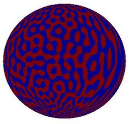
Figure 1. A nodal picture of a spherical harmonic. The blue and red are positive and negative domains respectively, and the nodal set is the interface between these.

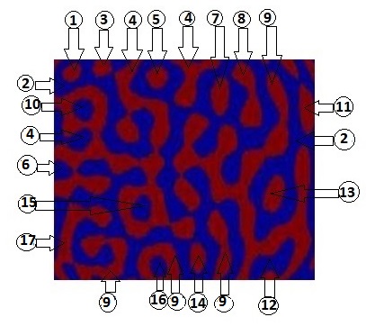
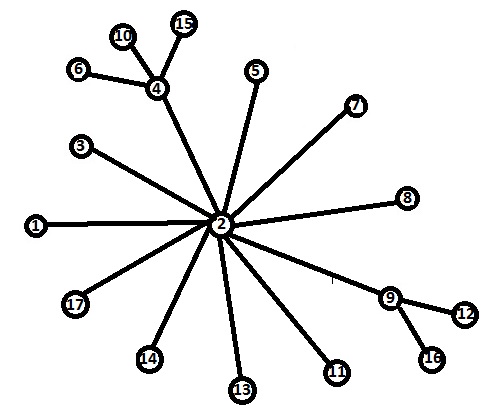
Figure 2. To the right: the nesting tree $X(f)$ corresponding to a fragment of the nodal picture in Figure 1, to the left, containing $17$ nodal domains (where we neglected some small ones lying next to the boundary). Figure 1 is essential for deciding which components merge on the sphere outside of the fragment.

As mentioned above, Nazarov and Sodin have determined the asymptotic law for the cardinality $|\mathcal{C}(f)|$ of $\mathcal{C}(f)$ as $T\rightarrow\infty$. There is a positive constant $\beta_{n,\alpha}$ depending on $n$ and $\alpha$ (and not on $\mathcal{M}$) such that, with probability tending to $1$ as $T\rightarrow\infty$,

(1.4) $$|\mathcal{C}(f)|\sim\beta_{n,\alpha}\frac{\omega_{n}}{(2\pi)^{n}}\operatorname{Vol}(\mathcal{M})T^{n},$$

here $\omega_{n}$ is the volume of the unit $n$-ball. We call these constants $\beta_{n,\alpha}$ the Nazarov-Sodin constants. Except for $n=1$ when the nodal set is a finite set of points and (1.4) can be established by the Kac-Rice formula ($\beta_{1,\alpha}=\frac{1}{\sqrt{3}}\cdot\sqrt{1+\alpha+\alpha^{2}}$), these numbers are not known explicitly.

In order to study the topologies of the components of $\mathcal{C}(f)$ and of the nesting trees $X(f)$, we introduce two measure spaces. Let $H(n-1)$ be the countable set of diffeomorphism types of compact $(n-1)$-dimensional manifolds that can be embedded in $\mathcal{S}^{n}$ and let $\mathcal{T}$ denote the set of finite rooted trees. As discrete spaces they carry measures, and define the discrepancy $D$ between $\mu$ and $\nu$ by

(1.5) $$D(\mu,\nu)=\sup\limits_{A}\left|\mu(A)-\nu(A)\right|,$$

where the supremum is taken w.r.t. all subsets $A$ of $H(n-1)$ (resp. $\mathcal{T}$).

Associating to $c\in\mathcal{C}(f)$ its topological type$t(c)$ gives a map from $\mathcal{C}(f)$ to $H(n-1)$. Similarly, each $c\in\mathcal{C}(f)$ is an edge in the tree $X(f)$ so that removing it leaves two rooted trees. We let $e(c)$ be the smaller one (if they are equal in size choose any one of them) and call it the end of $X(f)$ corresponding to $c$. Hence $e$ gives a map from $\mathcal{C}(f)$ to $\mathcal{T}$.

With these associations we define the key probability measures $\mu_{\mathcal{C}(f)}$ and $\mu_{X(f)}$ which measure the distribution of the topologies of the components of $V(f)$ and of the nesting ends of $X(f)$ by

(1.6) $$\mu_{\mathcal{C}(f)}:=\frac{1}{|\mathcal{C}(f)|}\sum\limits_{c\in\mathcal{C}(f)}\delta_{t(c)}$$

and

(1.7) $$\mu_{X(f)}:=\frac{1}{|\mathcal{C}(f)|}\sum\limits_{c\in\mathcal{C}(f)}\delta_{e(c)},$$

where $\delta_{\xi}$ is a point mass at $\xi$.

1.3. Statement of the main result

Our main result is that as $T\rightarrow\infty$ and for typical $f\in\mathcal{E}_{\mathcal{M},\alpha}(T)$ the above measures converge to Universal Laws (that is probability measures) on $H(n-1)$ and $\mathcal{T}$ respectively:

Theorem 1.1.

1. There are universal probability measures $\mu_{\mathcal{C},n,\alpha}$ on H(n-1) and $\mu_{X,n,\alpha}$ on $\mathcal{T}$, depending only on $n$ and $\alpha$ but not on $\mathcal{M}$, such that for every $\epsilon>0$,

   (1.8) $$\mathcal{P}\left\{f\in\mathcal{E}_{\mathcal{M},\alpha}(T):\>\max\left[D(\mu_{\mathcal{C}(f)},\mu_{\mathcal{C},n,\alpha}),D(\mu_{X(f)},\mu_{X,n,\alpha})\right]>\epsilon\right\}$$

   tends to $0$ as $T\rightarrow\infty$.

2. The support of $\mu_{\mathcal{C},n,\alpha}$ is

   $$\operatorname{supp}\mu_{\mathcal{C},n,\alpha}=H(n-1)$$

   and the support of $\mu_{X,n,\alpha}$ is

   $$\operatorname{supp}\mu_{X,n,\alpha}=\mathcal{T}.$$

Remark 1.2.

The most difficult case of part (2) of Theorem 1.1 is the monochromatic case $\alpha=1$. The proof of this for $n>2$ is given in the companion paper  [C-S].

Remark 1.3.

Though formulated for the sphere with arbitrary smooth metric, Theorem 1.1 holds on general compact smooth Riemannian manifolds with no boundary. Though the Jordan-Brouwer Theorem might fail for other manifolds (hence the nesting graph might fail to be a tree), it still holds locally, which is sufficient for all our needs.

The measures $\mu_{\mathcal{C}(f)}$ and $\mu_{X(f)}$ carry a lot of information. If

$$F:H(n-1)\rightarrow P$$

is a $P$-valued topological invariant then one can define the $P$-distribution of

$$f\in\mathcal{E}_{\mathcal{M},\alpha}(T)$$

to be

$$\mu_{F(f)}=\frac{1}{|\mathcal{C}(f)|}\sum\limits_{c\in\mathcal{C}(f)}\delta_{F(t(c))},$$

i.e. $\mu_{F(f)}$ is the pushforward of $\mu_{\mathcal{C}(f)}$ to $P$. Theorem 1.1 then gives the universal distribution of $\mu_{F(f)}$, namely it is simply the pushforward of $\mu_{\mathcal{C},n,\alpha}$. The same applies to any $Q$-valued map $G:\mathcal{T}\rightarrow Q$. Of special interest in this connection are Betti distributions and domain connectivities.

The first is the vector of Betti numbers given by

$$F(c)=\text{Betti}(c)=(\beta_{1}(c),\ldots,\beta_{k}(c)),$$

where $\beta_{j}(c)$ is the $j$-th Betti number of $c$. Here we are assuming $n=2k$ or $2k+1$ with $k>0$ (these Betti numbers give the rest since $c$ is connected and applying Poincaré duality). The image of $H(n-1)$ under $F$ can be shown to be $P_{n}$, which is $(\mathbb{Z}_{\geq 0})^{k}$ if $n$ is odd and $(\mathbb{Z}_{\geq 0})^{k-1}\times(2\mathbb{Z}_{\geq 0})$ if $n$ is even. Thus Theorem 1.1 yields the universal distribution of the vector of Betti numbers according to a Law $\mu_{\text{Betti},\alpha,n}$ on $P_{n}$ and whose support is $P_{n}$. We show that $\mu_{\text{Betti},\alpha,n}$ has finite total mean (which is not a formal consequence of Theorem 1.1):

$$\sum\limits_{y\in P_{n}}\left(\sum\limits_{j=1}^{k}y_{j}\right)\mu_{\text{Betti},n,\alpha}\left(\left\{y\right\}\right)<\infty.$$

For the domain connectivity distributions let $G:\mathcal{T}\rightarrow\mathbb{N}$ be the function which assigns to each rooted tree one plus the degree (i.e. number of neighbours) of the root. Now the root of $e(c)$ in $\mathcal{T}$ corresponds to a nodal domain $\omega$ of $f$, and $G(e(c))$ is the connectivity $m(\omega)$ of $\omega$, that counts the number of its boundary components. The measure $\mu_{G(f)}$ is essentially the connectivity measure:

(1.9) $$\mu_{\Gamma(f)}:=\frac{1}{|\Omega(f)|}\sum\limits_{\omega\in\Omega(f)}\delta_{m(\omega)}$$

on $\mathbb{N}$.

Theorem 1.1 yields a universal distribution for these connectivities according to a Law $\mu_{\Gamma,n,\alpha}$ on $\mathbb{N}$, and whose support is $\mathbb{N}$. Since the means over $\mathbb{N}$ of each measure in (1.9) is (see §2.4)

$$2-\frac{2}{|\Omega(f)|},$$

it follows that the mean of the law $\mu_{\Gamma,n,\alpha}$ is at most $2$.

1.4. Applications

The extreme values of $\alpha$, namely $0$ and $1$ are the most interesting. The case $\alpha=1$ is the monochromatic random wave (and also corresponds to random spherical harmonics) and it has been suggested by Berry [Be] that it models the individual eigenstates of the quantization of a classically chaotic Hamiltonian. The examination of the count of nodal domains (for $n=2$) in this context was initiated by  [B-G-S], and  [B-S], and the latter suggest some interesting possible connections to exactly solvable critical percolation models.

The law $\mu_{\Gamma,2,1}$ gives the distribution of connectivities of the nodal domains for monochromatic waves. Barnett and Jin’s numerical experiments  [B-J] give the following values for its mass on atoms.

connectivity	1	2	3	4	5	6	7
$\mu_{\Gamma,2,1}$	.91171	.05143	.01322	.00628	.00364	.00230	.00159

connectivity	8	9	10	11	12	13	14
$\mu_{\Gamma,2,1}$	.00117	.00090	.00070	.00058	.00047	.00039	.00034

connectivity	15	16	17	18	19	20	21
$\mu_{\Gamma,2,1}$	.00030	.00026	.00023	.00021	.00018	.00017	.00016

connectivity	22	23	24	25	26
$\mu_{\Gamma,2,1}$	.00014	.00013	.00012	.000098	.000097

The case $\alpha=0$ corresponds to the algebro-geometric setting of a random real projective hypersurface. Let $W_{n+1,t}$ be the vector space of real homogeneous polynomials of degree $t$ in $n+1$ variables. For $f\in W_{n+1,t}$, $V(f)$ is a real projective hypersurface in $\mathbb{P}^{n}(\mathbb{R})$. We equip $W_{n+1,t}$ with the “real Fubini-Study” Gaussian coming from the inner product on $W_{n+1,t}$ given by

(1.10) $$\langle f,\,g\rangle=\int\limits_{\mathbb{R}^{n+1}}f(x)g(x)e^{-|x|^{2}/2}dx$$

(the choice of the Euclidian length $|x|$ plays no role  [Sa]). This ensemble is essentially $\mathcal{E}_{\mathcal{M},0}(t)$ with $\mathcal{M}=(\mathcal{S}^{n},\sigma)$ the sphere with its round metric (see  [Sa]).

Thus the laws $\mu_{\mathcal{C},n,0}$ describe the universal distribution of topologies of a random real projective hypersurface in $\mathbb{P}^{n}$ (w.r.t. the real Fubini-Study Gaussian). It is interesting to compare this with the more familiar case of complex hypersurfaces. For those the generic (i.e. on a Zariski open set) hypersurface is smooth connected and of a fixed topology. Over $\mathbb{R}$ these hypersurfaces are very complicated and have many components. The main theorem asserts that if “generic” is replaced by “random” then order is restored in that the distribution of the topologies and Betti numbers is universal, at least when $t\rightarrow\infty$.

If $n=2$ the Nazarov-Sodin constant $\beta_{2,0}$ is such that the random oval is about $4\%$ Harnack, that is it has about $4\%$ of the maximal number of components that it can have ( [Na], [Sa]). The measure $\mu_{\Gamma,2,0}$ gives the distribution of the connectivities of the nodal domains of a random oval. Barnett and Jin’s Montre-Carlo simulation for these yields:

connectivity	1	2	3	4	5	6	7
$\mu_{\Gamma,2,0}$	.94473	.02820	.00889	.00437	.00261	.00173	.00128

connectivity	8	9	10	11	12	13	14
$\mu_{\Gamma,2,0}$	.00093	.00072	.00056	.00048	.00039	.00034	.00029

connectivity	15	16	17	18	19	20	21
$\mu_{\Gamma,2,0}$	.00026	.00025	.00021	.00019	.00016	.00014	.00013

connectivity	22	23	24	25	26
$\mu_{\Gamma,2,0}$	.00011	.00011	.00009	.00008	.00008

From these tables it appears that the decay rates of $\mu_{\Gamma,2,1}(\{m\})$ and $\mu_{\Gamma,2,0}(\{m\})$ for $m$ large are power laws $m^{-\gamma}$, with $\gamma$ approximately $2.149$ for $\alpha=1$ and $2.057$ for $\alpha=0$. These are close to the universal Fisher constant $187/91$ which governs related quantities in critical percolation  [K-Z].

We note that the only cases for which there is an explicit description of $H(n-1)$ are $n=2$ and $n=3$. For $n=2$ $H(n-1)$ is a point, namely the circle $\mathcal{S}^{1}$. For $n=3$, $H(2)$ consists of all the orientable compact surfaces and these are determined by their genus $g$, a non-negative integer. Thus $H(2)=\mathbb{Z}_{\geq 0}$, and $\mu_{\mathcal{C},3,\alpha}$ is a measure on $\mathbb{Z}_{\geq 0}$ which has finite mean (see §2). It would be very interesting to Monte-Carlo the distributions $\mu_{\mathcal{C},3,0}$ and $\mu_{\mathcal{C},3,1}$ and to learn more about their profiles. The only features that we know about the Universal Laws are that they are probability measures and that they charge every atom and in some special case that their “means” are finite.

1.5. Outline of the paper

We turn to an outline of the proof of Theorem 1.1, and also the content of the various sections. Most probabilistic calculations for the Gaussian Ensembles $\mathcal{E}_{\mathcal{M},\alpha}(T)$ start with the covariance kernel

(1.11) $$K_{\alpha}(T;x,y):=\mathbb{E}_{\mathcal{E}}[f(x)f(y)]=\sum\limits_{\alpha T\leq t_{j}\leq T}\phi_{j}(x)\phi_{j}(y)$$

(with suitable modifications if $\alpha=1$).

The behaviour of $K_{\alpha}$ as $T\rightarrow\infty$ is decisive in the analysis and it can be studied using micro-local analysis and the wave equation on $\mathcal{M}\times\mathbb{R}$, see section 2 for more details. We have

(1.12) $$\widetilde{K_{\alpha}}(T;x,y):=\frac{1}{D_{\alpha}(T)}K_{\alpha}(T;x,y)=B_{n,\alpha}(T\cdot d(x,y))+O\left(T^{-1}\right)$$

uniformly for $x,y\in\mathcal{M}$, where $d(x,y)$ is the (geodesic) distance in $\mathcal{M}$ between $x$ and $y$,

$$D_{\alpha}(T)=\frac{1}{\operatorname{Vol}(\mathcal{M})}\int\limits_{\mathcal{M}}K_{\alpha}(T;x,x)d\operatorname{Vol}(x),$$

and for $w\in\mathbb{R}^{n}$

(1.13) $$B_{n,\alpha}(w)=B_{n,\alpha}(|w|)=\frac{1}{|A_{\alpha}|}\int\limits_{A_{\alpha}}e(\langle w,\xi\rangle)d\xi$$

with

$$A_{\alpha}=\left\{w:\>\alpha\leq|w|\leq 1\right\}.$$

Thus for $x$ and $y$ roughly $1/T$ from each other $\widetilde{K_{\alpha}}$ is approximated by the universal kernel $B_{n,\alpha}$, whereas of $x$ and $y$ are a bit further apart, then the correlation is small.

The estimate (1.12) allows one to compute local quantities for the typical $f$ in $\mathcal{E}_{\mathcal{M},\alpha}(T)$, for example, the density of critical points (see the ‘Kac-Rice’ formula in section 2), or the $(n-1)$-dimensional volume of $V(f)$. While these are interesting and, in fact, useful for us, for example in bounding from above the Betti numbers using Morse Theory, the topology of $V(f)$ is global and lies beyond these purely local quantities. It was a major insight of Nazarov and Sodin  [So] that most components $c$ of $V(f)$ and $\omega$ of $\Omega(f)$ are small, that is are of diameter at most $O(1/T)$, and that the components that are further than this scale of $1/T$ apart are (almost) independent. This simultaneously semi-localizes the problem of the distribution of the topologies, and also explains the concentration feature that most $f$’s have the same distribution as well as the universality.

Moreover it separates the analysis into different parts. The first being the study of the problem for the scaling limits determined by (1.12) and (1.13). We call these the “scale invariant models”, and they are translation invariant isotropic Gaussian fields on $\mathbb{R}^{n}$ determined by (1.13). We denote them by $\mathfrak{g}_{n,\alpha}$ and review their properties in section 2. Once these are understood one has to couple the scale invariant theory with the global analysis after decomposing $\mathcal{M}$ into pieces of size $1/T$.

In section 2 we review some ‘standard’ theory such as properties of the fields $\mathfrak{g}_{n,\alpha}$, the Kac-Rice formula and some elementary topology. Sections 3, 4 and 5 are concerned with proving the analogue of Theorem 1.1 for the fields $\mathfrak{g}_{n,\alpha}$. The measure spaces $H(n-1)$ and $\mathcal{T}$ are non-compact so that weak limits of probability measures need not be probability measures. In terms of technical novelty this issue is a central one for us. In section 3 we prove the existence as weak limits of $\mu_{\mathcal{C},n,\alpha}$ and $\mu_{X,n,\alpha}$ associated with the $\mathfrak{g}_{n,\alpha}$’s. The proof is relatively soft and follows closely the component counting analysis of [N-S] and  [So]. The main difference is that our random variables are conditioned to count a given topological type (respectively tree end). This requires a number of modifications and extensions, especially of various inequalities (see §3.2, §6.4, §7.4).

Section 4 is devoted to a proof that the universal limit measures $\mu_{\mathcal{C},n,\alpha}$ and $\mu_{X,n,\alpha}$ are in fact probability measures. This requires establishing some tightness properties for the tails of our families of measures (see Proposition 4.3). The Kac-Rice formula allows us to show that most components $c$ of a typical $V(f)$ are gotten from $\mathcal{S}^{n-1}$ with a bounded number of surgeries. However this is not sufficient to control their topologies uniformly. To limit these we examine further the geometries of the components. We show that for most components there are uniform bounds from above for their volumes, diameter and curvatures. With this, versions of Cheeger’s finiteness theorem (see Lemma 4.4 in §4.2) allows us to restrict their topological types and hence to establish the desired tightness property. For the case of tree ends a similar but much simpler analysis gives the desired control on the geometry of nodal domains, yielding the corresponding tightness.

Section 5 is concerned with a proof that for the $\mathfrak{g}_{n,\alpha}$’s the limit measures $\mu_{\mathcal{C},n,\alpha}$ and $\mu_{X,n,\alpha}$ have full support (i.e. that they charge every atom). For the cases $0\leq\alpha<1$ this is straightforward (see §5.2). The case $\alpha=1$ presents us with a second technically novel problem. We resolve it for $n=2$ and for the measure $\mu_{X,2,1}$ in this section. This makes use of some auxiliary lemmas about approximating functions in $C(K)$, $K\subseteq\mathbb{R}^{2}$ compact, by solutions $u$ of

$$\Delta u+u=0$$

in $\mathbb{R}^{2}$. This is combined with a combinatorial analysis of the zero sets of perturbations of

$$u(x_{1},x_{2})=\sin(x_{1})\cdot\sin(x_{2}).$$

The general case of the support of these measures for $n\geq 3$ is established in the companion paper  [C-S].

Section 6 gives ‘semi-local’ analysis concerning the $\mathfrak{g}_{n,\alpha}$’s with a decomposition of $\mathcal{M}$ into pieces at scale $1/T$ to study the typical members of $\mathcal{E}_{\mathcal{M},\alpha}(T)$. Section 7 ends with a proof of Theorem 1.1 by combining or ‘gluing’ the ‘semi-local’ pieces of $\mathcal{M}$. Again we follow closely the analysis of the counting of the number of components in  [N-S] and  [So]. This requires a number of modifications and extensions (for example see the proof of Proposition 6.8 in §6.4 or the proof of Proposition 7.2 in §7.4), and we spell these out in some detail.

1.6. Acknowledgements

We would like to thank Mikhail Sodin for sharing freely early versions of his work with Fedor Nazarov and in particular for the technical discussions with one of us (Wigman) in Trondheim 2013, and Zeév Rudnick for many stimulating discussions. In addition I.W. would like to thank Dmitri Panov and Yuri Safarov for sharing their expertise on various topics related to the proofs. We also thank Alex Barnett for carrying out the numerical experiments connected with this work and for his figures which we have included, as well as P. Kleban and R. Ziff for formulating and examining the “holes of clusters” in percolation models. We are grateful to Nalini Anantharaman, Yaiza Canzani and Curtis McMullen for their valuable comments on some earlier versions of this manuscript and to S. Weinberger for clarifying issues of decidability of topological types in higher dimensions. Finally, it is a pleasure to thank the anonymous referee for his careful reading and constructive criticism on an earlier version of this manuscript, that, in particular, improved its readability significantly.

2. Basic conventions

We review some material that will be used in the text. We begin with a quantitative local Weyl law for $\mathcal{M}$.

2.1. Quantitative local Weyl law

The modern treatments of Weyl’s law with remainder involve construction of a parametrix for the wave equation on $\mathcal{M}\times\mathbb{R}$ as developed first in  [Lax] and  [Horm]. For the spectral window that we treat a parametrix for a small fixed time interval suffices. The recent papers  [C-H] and  [C-H2], which we will use as a reference, go beyond what we need in that they allow $\eta(T)$ to be bounded in the case $\alpha=1$. Their goal is a remainder term of $o(T^{n-1})$, and for that they assume some properties of the geodesic flow. Since we assume that $\eta(T)\rightarrow\infty$ (in fact, that $\eta(T)=T^{\beta}$ for some $0<\beta<\frac{1}{2}$) and we are content with a bound of $O(T^{n-1})$ for the remainder, the analysis from  [C-H] and  [C-H2] is simpler, and we don’t need to impose any conditions on $\mathcal{M}=(\mathcal{S}^{n},g)$.

Specifically, as pointed out in equation (5) of  [C-H2], the remainder $R(x,y,T)$ (our $T$ is their $\lambda$) in their equation (4) is $O(T^{n-1})$, and this is proved without any assumptions on the geodesic flow (see Theorem $4.4$ of  [Horm]). In their analysis of the main term in (4) leading to their Theorem $1$, there is a parameter $\epsilon$, which they allow to go to zero, and which makes use of the non self-focal condition. If we fix $\epsilon$ a large constant so that the parametrix constructed in their section $2$ is used only for $|t|<\frac{1}{\epsilon}$, then no condition on the geodesic flow are used and one obtains their Theorem $1$ with the weaker $O(1)$ replacing their $o(1)$. This leads to: uniformly for $x,y\in\mathcal{M}$

$$\begin{split}K_{T}(x,y)&:=\sum\limits_{t_{j}\leq T}\phi_{j}(x)\phi_{j}(y)\\ &=T^{n}B_{n}(T\cdot d(x,y))+O(T^{n-1}),\end{split}$$

where

$$B_{n}(w)=B_{n}(|w|)=\int\limits_{|\xi|\leq 1}e(\langle w,\xi\rangle)d\xi.$$

Hence if $0\leq T^{\prime}<T$,

(2.1) $$\begin{split}K_{T}(x,y)-K_{T^{\prime}}(x,y)&=\sum\limits_{T^{\prime}\leq t_{j}\leq T}\phi_{j}(x)\phi_{j}(y)\\ &=T^{n}B_{n,T^{\prime}/T}(T\cdot d(x,y))+O(T^{n-1}),\end{split}$$

where

$$B_{n,\gamma}(w)=\int\limits_{\gamma\leq|\xi|\leq 1}e(\langle w,\xi\rangle)d\xi.$$

In particular if $0\leq\alpha<1$ is fixed then we obtain the desired Weyl asymptotics that we will use for the $\mathcal{E}_{\mathcal{M},\alpha}(T)$’s.

For the monochromatic case $\alpha=1$,

$$T^{\prime}/T=1-\eta(T)/T=1-T^{\beta-1},$$

and hence

(2.2) $$\begin{split}&K_{T}(x,y)-K_{T^{\prime}}(x,y)\\ &=n\eta(T)T^{n-1}B_{n,1}(T\cdot d(x,y))+O\left(T^{n-1}+\eta^{2}T^{n-2}(Td(x,y))\right),\end{split}$$

where

$$B_{n,1}(w)=B_{n,1}(|w|)=\int\limits_{|\xi|=1}e(\langle w,\xi\rangle)d\nu_{1}(\xi),$$

and $\nu_{1}$ is the spherical Haar measure on $\mathcal{S}^{n-1}$. We need also to control the derivatives of $K_{T}(x,y)$ w.r.t. $x$ and $y$ when $x$ and $y$ are very close (within $1/T$ of each other). Using geodesic normal coordinates about a point $x_{0}$ in $\mathcal{M}$ and the exponential map from $T_{x_{0}}(\mathcal{M})$ identified with $(\mathbb{R}^{n},0)$ to $\mathcal{M}$,  [C-H] show say in the case $\alpha=1$ (which is the most difficult one) that

(2.3) $$K_{T}\left(\exp_{x_{0}}\left(\frac{u}{T}\right),\exp_{x_{0}}\left(\frac{v}{T}\right)\right)=n\eta T^{n-1}B_{n,1}(u-v)+O(T^{n-1}),$$

and this holds uniformly together with any fixed number of derivatives w.r.t. $u$ and $v$. They establish this for $\mathcal{M}$ real analytic in  [C-H], and for the general $C^{\infty}$-case in  [C-H2].

Our discussion above does not apply directly to the interesting special case of $\mathcal{M}$ being the standard round sphere $\mathcal{S}^{n}$ and $\mathcal{E}_{\mathcal{M},1}(T)$ being the space of spherical harmonics of a given degree. In that case the classical Mehler-Heine asymptotics for Gegenbauer polynomials yield a version of (2.3), and all the results in this paper apply equally well to these “monochromatic waves”.

2.2. Scale invariant fields

The semi-classical approximations (2.1), (2.2) and (2.3) lead to the study of the scaled Gaussian fields at a point $x_{0}\in\mathcal{M}$, and these in turn to the scale invariant Gaussian fields $\mathfrak{g}_{n,\alpha}$ on $\mathbb{R}^{n}$. They are defined as follows.

Let $\psi_{j}$, $j=1,2,\ldots$ be a real valued o.n.b. of $L^{2}(A_{\alpha},d\nu_{\alpha})$ with $0\leq\alpha<1$ and $L^{2}(\mathcal{S}^{n-1},d\nu_{1})$ if $\alpha=1$ (here $A_{\alpha}$ is the annulus $\alpha\leq|\xi|\leq 1$ and $d\nu_{\alpha}$ its Haar measure). Set

$$\widehat{\psi_{j}}=\int\limits_{\mathbb{R}^{n}}\psi_{j}(\xi)e(\langle x,\xi\rangle)d\nu_{\alpha}:=C_{j}(x)+S_{j}(x)$$

to be the real valued cosine and sine transforms. Define a random $f(x)$ by

(2.4) $$f(x)\sim\sum\limits_{j=1}^{\infty}(a_{j}C_{j}(x)+b_{j}S_{j}(x)),$$

where $a_{j},b_{j}$ are independent $N(0,1)$ Gaussian variables. The space of such $f$’s is denoted by $G_{n,\alpha}$, and the corresponding probability measure on the measurable subsets of $G_{n,\alpha}$ by $P_{n,\alpha}$. The Gaussian fields $\mathfrak{g}_{n,\alpha}$ are then $(G_{n,\alpha},P_{n,\alpha})$.

From the definitions one checks that for $x,y\in\mathbb{R}^{n}$,

(2.5) $$\begin{split}&\sum\limits_{j=1}^{\infty}\left(C_{j}(x)C_{j}(y)+S_{j}(x)S_{j}(y)\right)=\int\limits_{\mathbb{R}^{n}}e(\langle x-y,\xi\rangle)d\nu_{\alpha}(\xi)\\ &=\widehat{\nu_{\alpha}}(x-y):=\operatorname{Cov}_{n,\alpha}(x-y):=\mathbb{E}_{f}[f(x)\cdot f(y)].\end{split}$$

It follows that $\mathfrak{g}_{n,\alpha}=(G_{n,\alpha},P_{n,\alpha})$ is a translation and rotation invariant random field ( [A-T, A-W]). That is, if $B$ is a (measurable) subset of $G_{n,\alpha}$, then

$$P_{n,\alpha}(B)=P_{n,\alpha}(RB)$$

for any rigid motion $R$ of $\mathbb{R}^{n}$ (here $Rf(x):=f(Rx)$). Moreover, since $\widehat{\nu_{\alpha}}(x)$ is analytic in $x$, almost all $f$’s in $G_{n,\alpha}$ represent analytic functions on $\mathbb{R}^{n}$. This follows for example from the series (2.4) converging uniformly on compacta in $x$ for a.a. choices of the Gaussian variables $a_{j}$, $b_{j}$, see Appendix A for more details.

Of special interest is $\alpha=1$ for which one can choose as o.n.b. of $L^{2}(\mathcal{S}^{n-1},\nu_{1})$ the special harmonic $Y_{m}^{l}$, $l\geq 0$ and $m=1,\ldots d_{l}$. A computation  [C-S] shows that the ensemble $\mathfrak{g}_{n,1}$ has a representation

$$f(x)\sim(2\pi)^{n/2}\sum\limits_{l=0}^{\infty}\sum\limits_{m=1}^{d_{l}}b_{l,m}Y_{m}^{l}\left(\frac{x}{|x|}\right)\frac{J_{l+\nu}(|x|)}{|x|^{\nu}}$$

with

$$\nu=\frac{n-2}{2}$$

and $b_{l,m}$ independent $N(0,1)$ Gaussians.

2.3. Kac-Rice

To illustrate the use of the covariance and its asymptotic approximation above, we review the computation of expected zero volume and or critical points number for random fields. These are computed using the “Kac-Rice” formula. Let $m\leq n$, $H:\mathcal{D}\rightarrow\mathbb{R}^{m}$ be a smooth random field on a domain $\mathcal{D}\subseteq\mathbb{R}^{n}$, and $\mathcal{Z}(H;\overline{\mathcal{D}})$ be either the $(n-m)$-volume of $H^{-1}(0)$ (for $m<n$), or the number of the discrete zeros (for $m=n$).

We set $J_{H}(x)$ to be the (random) Jacobi matrix of $H$ at $x$ and define the “zero density” of $H$ at $x\in\mathcal{D}$ as the conditional Gaussian expectation

(2.6) $$K_{1}(x)=K_{1;H}(x)=\varphi_{H(x)}(0)\cdot\mathbb{E}[|\det J_{H}(x)|\big{|}H(x)=0],$$

where $\varphi_{H(x)}(0)$ is the probability density function of $H(x)$ evaluated at $0\in\mathbb{R}^{m}$. With the notation above the Kac-Rice formula (meta-theorem) states that, under some non-degeneracy condition on $H$,

$$\mathbb{E}[\mathcal{Z}(H;\mathcal{D})]=\int\limits_{\mathcal{D}}K_{1}(x)dx.$$

Concerning the sufficient conditions that guarantee that (2.6) holds, a variety of results is known  [A-T, A-W]. The following version of Kac-Rice merely requires the non-degeneracy of the values of $H(x)$ (vs. the non-degeneracy of $(H(x),J_{H}(x))$ in the appropriate sense, as in the other sources), to our best knowledge, the mildest sufficient condition.

Lemma 2.1 (Standard Kac-Rice  [A-W], Theorem $6.3$).

Let $H:\mathcal{D}\rightarrow\mathbb{R}^{m}$ be an a.s. smooth Gaussian field, such that for every $x\in\mathcal{D}$ the distribution of the random vector $H(x)\in\mathbb{R}^{m}$ is non-degenerate Gaussian. Then

(2.7) $$\mathbb{E}[\mathcal{Z}(H;\mathcal{D})]=\int\limits_{\mathcal{D}}K_{1}(x)dx$$

with the zero density $K_{1}(x)$ as in (2.6).

The Gaussian density (2.6) is a Gaussian integral that, in principle, could be evaluated explicitly. However, in practice, it is not easy to control $K_{1}(x)$ uniformly in both $x$ and the field $H$. The following lemma was proved in  [So]; it offers an easy and explicit upper bound for the discrete number of zeros (in case $m=n$), uniformly w.r.t. $H$.

Lemma 2.2 ([So, Lemma $2$]).

Let $m\geq 1$, $B\subseteq\mathbb{R}^{m}$ a ball and $H:\overline{B}\rightarrow\mathbb{R}^{m}$ an a.s. $C^{1}$-smooth random Gaussian field. Then we have

(2.8) $$\mathbb{E}[\mathcal{Z}(H;\overline{B})]\leq C\sup\limits_{x\in\overline{B}}\frac{\mathbb{E}[|\nabla H(x)|^{2}]^{m/2}}{(\det\mathbb{E}[H(x)\cdot H(x)^{t}])^{1/2}}\cdot\operatorname{Vol}(B).$$

for some universal constant $C=C(m)>0$, where

$$|\nabla H(x)|^{2}=\sum\limits_{i,j}|\partial_{i}H_{j}|^{2}$$

is the Hilbert-Schmidt norm.

Note that both the denominator and the numerator of the r.h.s. of (2.8) may be expressed in terms of the covariance matrix $(r_{ij}(x,x))_{ij}$ and its second mixed derivatives $(\partial_{lm}r_{ij}(x,x))_{ijlm}$ evaluated on the diagonal $x=y$. If $H$ is stationary, then the fraction on the r.h.s. of (2.8) does not depend on $x$, so that in the latter case (2.8) is

(2.9) $$\mathbb{E}[\mathcal{Z}(H;\overline{B})]\leq C(H)\cdot\operatorname{Vol}(B)$$

with $C(H)$ expressed in terms of the covariance of $H$ and a couple of its derivatives at the origin $x=0$.

We now apply Lemma 2.2 for counting critical points of a given stationary field $F$ by using $H=\nabla F$.

Corollary 2.3 (Kac-Rice upper bound).

Let $\mathcal{D}\subseteq\mathbb{R}^{m}$ be a domain and $F:\mathcal{D}\rightarrow\mathbb{R}^{m}$ an a.s. $C^{2}$-smooth stationary Gaussian random field, such that for $x\in\mathcal{D}$ the distribution of $\nabla F(x)$ is non-degenerate Gaussian.

1. For $r>0$ let $\mathcal{A}(F;r)$ be the number of critical points of $F$ inside $B(r)\subseteq\mathcal{D}$. Then

   $$\mathbb{E}[\mathcal{A}(F;r)]=O(\operatorname{Vol}(B(r))),$$

   where the constant involved in the ‘$O$’-notation depends on the law of $F$ only.

2. For $r>0$ let $\widetilde{\mathcal{A}}(F;r)$ be the number of critical points of the restriction $F|_{\partial B(r)}$ of $F$ to the sphere $\partial B(r)\subseteq\mathcal{D}$. Then

   $$\mathbb{E}[\widetilde{\mathcal{A}}(F;r)]=O(\operatorname{Vol}(\partial B(r))),$$

   where the constant involved in the ‘$O$’-notation depends on the law of $F$ only.

Note that the total number $\mathcal{N}_{\mathcal{C}}(F;r,u)$ of nodal components of $F$ lying in $B_{u}(r)$ is bounded by the number $\mathcal{A}(F;r,u)$ of critical points of $F$ in $B_{u}(r)$. Hence Corollary 2.3 allows us to control the expected number of the former by the volume of the ball $B(r)$ (bearing in mind the stationarity of $F$). Similarly, the second part of Corollary 2.3 allows us to control the expected number of nodal components intersecting $\partial B_{u}(r)$ in terms of the volume of $\partial B_{u}(r)$. This approach is pursued in §3.3.

Proof of Corollary 2.3.

The first part of Corollary 2.3 is merely an application of (2.9) (following from Lemma 2.2) on the stationary field $H=\nabla F$. For the second part we decompose the sphere $\partial B(r)$ into (universally) finitely many coordinate patches, thus reducing the problem to the Euclidian case, and apply Lemma 2.2 on the restrictions of the gradient of $F|_{\partial B(r)}$ on each of the coordinate patches separately. Note that the total volume is of the same order of magnitude $r^{n-1}$ as $\partial B(r)$, so that the second statement of the present corollary follows from summing up the individual estimates (2.8), bearing in mind that upon passing to the Euclidian coordinates we are losing stationarity of the underlying random field (though the non-degeneracy of the gradient stays unimpaired).

∎

2.4. Some remarks on topology of $V(f)$

We end this background material section with some elementary remarks about the topology of $V(f)$. For the random $f\in\mathcal{E}_{T,\alpha}(\mathcal{M})$ (and $T$ large) a component $c$ of $V(f)$ is a smooth hypersurface in $\mathcal{S}^{n}$; hence it can be embedded in $\mathbb{R}^{n}$ and gives a point in $H(n-1)$. It is known that $c$ separates $\mathcal{S}^{n}$ into two connected components  [Li]. From this it follows that the nesting graph $X(f)$ is a tree and that

$$|X(f)|=|\Omega(f)|=|E(X(f))|+1=|\mathcal{C}(f)|+1.$$

The mean of the connectivity measure $\mu_{\Gamma(f)}$ from (1.9) is equal to

$$\sum\limits_{m=1}^{\infty}m\cdot\mu_{\Gamma(f)}(m)=\frac{1}{|\Omega(f)|}\sum\limits_{v\in X(f)}d(v),$$

where $d(v)$ is the degree of $v$. Now

$$2|E(X(f))|=\sum\limits_{v\in X(f)}d(v),$$

and hence

$$\sum\limits_{m=1}^{\infty}m\cdot\mu_{\Gamma(f)}(m)=\frac{2|E(X(f))|}{|\Omega(f)|}=2-\frac{2}{|\Omega(f)|}.$$

It follows that the means of the universal domain connectivity measures $\mu_{\Gamma,n,\alpha}$ are at most $2$. We do not know whether these are equal to $2$ or not.

The proof that the universal Betti measures $\mu_{\text{Betti},\alpha,n}$ (page 1.3) has finite (total) mean also follows from a finite individual bound. If $\mathcal{M}$ is $\mathcal{S}^{n}$ with its round metric, the eigenfunctions are spherical harmonics and any element of $\mathcal{E}_{\mathcal{M},\alpha}(T)$ is a homogeneous polynomial of degree $t=t(T)$. According to  [Mi] the total Betti number of the full zero set $V(f)$ of $f$ (which we can assume is nonsingular) is at most $t^{n}$. Nazarov and Sodin’s Theorem (1.4) asserts that the number of connected components of a typical $V(f)$ for $f$ in $\mathcal{E}_{\mathcal{M},\alpha}(T)$ is $c_{n,\alpha}\cdot t^{n}$, from which the finiteness of the total mean of the $\mu_{\text{Betti},\alpha,n}$ on $(\mathbb{Z}_{\geq 0})^{k}$ follows.

3. Scale-invariant model

3.1. Statement of the main result

Let $F:\mathbb{R}^{n}\rightarrow\mathbb{R}$ be an a.s. smooth stationary Gaussian random field. Here the relevant limit is considering the restriction $F|_{B(R)}$ of $F$ to the centred radius-$R$ ball $B(R)$, and taking $R\rightarrow\infty$. The covariance function of $F$ is $r_{F}:\mathbb{R}^{n}\times\mathbb{R}^{n}\rightarrow\mathbb{R}$, defined by the standard abuse of notation as

$$r_{F}(x,y)=r_{F}(x-y)=\mathbb{E}[F(x)F(y)],$$

and the spectral measure (density) $d\rho_{F}$ is the Fourier transform of $r_{F}$ on $\mathbb{R}^{n}$.

Notation 3.1.

Let $\Gamma\subseteq\mathbb{R}^{n}$ be a (deterministic) smooth hypersurface and $R>0$ a (large) parameter.

1. For $H\in H(n-1)$ let $\mathcal{N}_{\mathcal{C}}(\Gamma,H;R)$ be the number of connected components of $\Gamma$ lying entirely in $B(R)$, diffeomorphic to $H$.

2. For $c\in\mathcal{C}(\Gamma)$ let $e(c)$ be the rooted subtree of $X(\Gamma)$ cut by $c$, with vertices corresponding to domains $\omega\in\Omega(\Gamma)$ lying inside $c$.

3. For $G\in\mathcal{T}$ let $\mathcal{N}_{X}(\Gamma,G;R)$ be the number of edges $c\in\mathcal{C}(f)$ in the nesting tree of $\Gamma$, corresponding to components $c\in\mathcal{C}(\Gamma)$ lying entirely in $B(R)$ with $e(c)$ isomorphic to $G$.

4. We use the shorthand

   $$\mathcal{N}_{\cdot}(F;\cdot,\cdot):=\mathcal{N}_{\cdot}(F^{-1}(0),\cdot,\cdot)$$

   in either of the cases above.

Our principal result of this section (Theorem 3.3 below) asserts that, under some assumptions on $F$, as $R\rightarrow\infty$, the numbers

$$\mathcal{N}_{\cdot}(F;\cdot,R),$$

suitably normalized, converge in mean (i.e. in $L^{1}$).

Definition 3.2 (Axioms on $F$).

1. The measure $d\rho$ has no atoms.

2. For some $p>6$,

   $$\int\limits_{\mathbb{R}^{n}}\|\lambda\|^{p}d\rho(\lambda)<\infty.$$

3. $\operatorname{supp}\rho$ does not lie in a linear hyperplane.

Axiom $(\rho 2)$ implies [A-W, page 30] that $F$ is a.s. $C^{3}$-smooth, and axiom $(\rho 3)$ implies that the distribution of $(F(x),\nabla F(x))$ is a.s. non-degenerate. Finally, axiom $(\rho 1)$ guarantees that the action of translations (or shifts) on $F$ are ergodic, which is a crucial ingredient in Nazarov-Sodin theory (see Theorem 3.4 below). From (2.5) it is clear that axioms $(\rho 1)$, $(\rho 2)$ and $(\rho 3)$ hold for the $\mathfrak{g}_{n,\alpha}$’s considered in §2.2.

For this scale-invariant model Nazarov and Sodin proved [So, Theorem $1$] that under axioms $(\rho 1)-(\rho 3)$ on $F$ there exists a constant $\beta=\beta(F)$ such that

(3.1) $$\mathbb{E}\left[\left|\frac{\mathcal{N}_{\mathcal{C}}(F;R)}{\operatorname{Vol}(B(R))}-\beta\frac{\omega_{n}}{(2\pi)^{n}}\right|\right]\rightarrow 0,$$

and in particular, for every $\epsilon>0$

(3.2) $$\mathcal{P}\left\{\left|\frac{\mathcal{N}_{\mathcal{C}}(F;R)}{\operatorname{Vol}(B(R))}-\beta\frac{\omega_{n}}{(2\pi)^{n}}\right|>\epsilon\right\}\rightarrow 0,$$

and gave some sufficient conditions on $F$ for the positivity of $\beta$. The following theorem refines the latter result; it will imply the existence of the limiting measures in Theorem 4.2, part (1) below.

Theorem 3.3 (cf. [So, Theorem $1$]).

Let $F:\mathbb{R}^{n}\rightarrow\mathbb{R}$ be a random field whose spectral density $\rho$ satisfies the axioms $(\rho 1)-(\rho 3)$ above. Then for every $H\in H(n-1)$ and $G\in\mathcal{T}$ there exist constants, $c_{\mathcal{C}}(H)=c_{\mathcal{C};F}(H)=c_{\mathcal{C};\rho}(H)$ and $c_{X}(G)=c_{X;F}(G)=c_{X;\rho}(G)$ so that as $R\rightarrow\infty$,

(3.3) $$\begin{split}&\mathbb{E}\left[\left|\frac{\mathcal{N}_{\mathcal{C}}(F,H;R)}{\operatorname{Vol}(B(R))}-c_{\mathcal{C};F}(H)\right|\right]\rightarrow 0,\\ &\mathbb{E}\left[\left|\frac{\mathcal{N}_{X}(F,G;R)}{\operatorname{Vol}(B(R))}-c_{X;F}(G)\right|\right]\rightarrow 0.\end{split}$$

The statement (3.3) is to say that, as $R\rightarrow\infty$, we have the limits

$$\frac{\mathcal{N}_{\cdot}(F,\cdot;R)}{\operatorname{Vol}(B(R))}\rightarrow c_{\cdot;F}(\cdot)$$

in $L^{1}$. Using the same methods as in the present manuscript (and  [So]) it is possible to prove that these limits also valid a.s.; however, we were not able to infer the analogues of the latter statement for the Riemannian case (1.2). The rest of the present section is dedicated to the proof of Theorem 3.3, eventually given in §3.3.

3.2. Integral-Geometric sandwiches

Let $\tau_{u}$ be the translation operator

$$\tau_{u}:\mathbb{R}^{n}\rightarrow\mathbb{R}^{n}$$

acting on (random) functions, by $(\tau_{u}F)(x)=F(x-u)$. More precisely, we consider a Gaussian random field $F:\mathbb{R}^{n}\rightarrow\mathbb{R}^{n}$ as a probability space $(\Delta=C(\mathbb{R}^{n}),\mathscr{A},\mathcal{P})$, where $\mathscr{A}$ is the $\sigma$-algebra generated by the cylinder sets of the form

$$\{f\in\Delta:\>f(x_{j})\in A_{j}:\>j=1,\ldots k\}$$

with some $x_{j}\in\mathbb{R}^{n}$, and intervals $A_{j}\subseteq\mathbb{R}$, $j=1,\ldots,k$, and $\mathcal{P}$ the corresponding Gaussian measure, as prescribed by Kolmogorov’s Theorem. Under axiom $(\rho 2)$, $\mathcal{P}$ is supported on the smooth functions (e.g. $C^{1}(\mathbb{R}^{n})$).

In this section we reduce the various nodal counts into a purely ergodic question; the latter is addressed using the following result (after Wiener, Grenander-Fomin-Maruyama, see  [So, Theorem 3] and references therein):

Theorem 3.4.

1. Let $F$ be a random stationary Gaussian field with spectral measure $d\rho$. Then if $d\rho$ contains no atoms, the action of the translations group

   $$(\tau_{u}F)(x)=F(x-u)$$

   is ergodic (“$F$ is ergodic”).

2. Suppose that $F$ is ergodic, and the translation map $\mathbb{R}^{n}\times C(\mathbb{R}^{n})\rightarrow C(\mathbb{R}^{n})$

   (3.4) $$(u,F)\mapsto\tau_{u}F$$

   is measurable w.r.t. the product $\sigma$-algebra $\mathscr{B}(\mathbb{R}^{n})\times\mathscr{A}$ and $\mathscr{A}$. Then every random variable $\Phi(F)$ with finite expectation $\mathbb{E}[|\Phi(F)|]<\infty$ satisfies

   $$\lim\limits_{R\rightarrow\infty}\frac{1}{\operatorname{Vol}(B(R))}\int\limits_{B(R)}\Phi(\tau_{u}F)du\rightarrow\mathbb{E}[\Phi(F)],$$

   convergence a.s. and in $L^{1}$.

To reduce the nodal counting questions into an ergodic question we formulate the Integral-Geometric Sandwich below. To present it it we need the following notation first.

Notation 3.5.

1. For $u\in\mathbb{R}^{n}$, $\Gamma$ a smooth hypersurface let

   $$\mathcal{N}_{\cdot}(\Gamma,\cdot;R,u):=\mathcal{N}_{\cdot}(\tau_{u}\Gamma,\cdot;R),$$

   i.e. the centred ball $B(R)$ in Notation 3.1 is replaced by $B_{u}(R)$, and use the shortcut

   $$\mathcal{N}_{\cdot}(F,\cdot;R,u):=\mathcal{N}_{\cdot}(F^{-1}(0),\cdot;R,u).$$

2. For each of the (random or deterministic) variables $\mathcal{N}_{\cdot}(\cdots)$ already defined, $\mathcal{N}_{\cdot}^{*}(\cdots)$ is defined along the same lines with “lying entirely in $B(R)$” replaced by “intersects $B(R)$”.

Remark 3.6.

Our approach will eventually show that the difference between

$$\mathcal{N}_{\cdot}(F,\cdot;R,u)$$

and

$$\mathcal{N}_{\cdot}^{*}(F,\cdot;R,u)$$

is typically negligible (see the proof of Theorem 3.3 below). It will imply “semi-locality”, i.e. that “most” of the nodal components (resp. tree ends) of $F$ are contained in balls of sufficiently big radius $R\gg 1$; bearing in mind the natural scaling these correspond to nodal components (resp. tree ends) of the band-limited functions $f$ in (1.2) lying in radius-$R/T$ geodesic balls on $\mathcal{M}$ (see also Lemma 7.4).

Lemma 3.7 (cf. [So, Lemma $1$]).

Let $\Gamma$ be a (deterministic) closed hypersurface. Then for $0<r<R$, $H\in H(n-1)$, $G\in\mathcal{T}$, one has

(3.5) $$\begin{split}&\frac{1}{\operatorname{Vol}(B(r))}\int\limits_{B(R-r)}\mathcal{N}_{\cdot}(\Gamma,\cdot;r,u)du\leq\mathcal{N}_{\cdot}(\Gamma,\cdot;R)\\ &\leq\frac{1}{\operatorname{Vol}(B(r))}\int\limits_{B(R+r)}\mathcal{N}_{\cdot}^{*}(\Gamma,\cdot;r,u)du\end{split}$$

with $\mathcal{N}_{\cdot}(\Gamma,\cdot;R)$ standing for $\mathcal{N}_{\mathcal{C}}(\Gamma,H;R)$ (resp. $\mathcal{N}_{X}(\Gamma,G;R)$), and similarly for the other counts involved in (3.5). That is, (3.5) asserts $2$ different sandwich inequalities corresponding to $\mathcal{N}_{\mathcal{C},X}(\cdots)$ respectively.

Proof.

We are only going to prove the sandwich inequality corresponding to $\mathcal{N}_{\mathcal{C}}$, namely that for $H\in H(n-1)$

(3.6) $$\begin{split}&\frac{1}{\operatorname{Vol}(B(r))}\int\limits_{B(R-r)}\mathcal{N}_{\mathcal{C}}(\Gamma,H;r,u)du\leq\mathcal{N}_{\mathcal{C}}(\Gamma,H;R)\\ &\leq\frac{1}{\operatorname{Vol}(B(r))}\int\limits_{B(R+r)}\mathcal{N}_{\mathcal{C}}^{*}(\Gamma,H;r,u)du,\end{split}$$

with the inequality for $\mathcal{N}_{X}$ proven along similar lines. Let $\gamma\subseteq B(R)$ be a connected component of $\Gamma$. Put

$$G_{*}(\gamma)=\bigcap\limits_{v\in\gamma}B(v,r)=\{u:\gamma\subseteq B(u,r)\}$$

and

$$G^{*}(\gamma)=\bigcup\limits_{v\in\gamma}\overline{B}(v,r)=\{u:\gamma\cap\overline{B(u,r)}\neq\emptyset\}.$$

We have for every $v\in\gamma$,

$$G_{*}(\gamma)\subseteq B_{v}(r)\subseteq G^{*}(\gamma),$$

and thus, in particular,

(3.7) $$\operatorname{Vol}(G_{*}(\gamma))\leq\operatorname{Vol}(B(r))\leq\operatorname{Vol}(G^{*}(\gamma)).$$

Summing up (3.7) for all components $\gamma\subseteq B(R)$ diffeomorphic to $H$, we obtain

(3.8) $$\begin{split}\sum\limits_{\begin{subarray}{c}\gamma\subseteq B(R)\\ \gamma\cong H\end{subarray}}\operatorname{Vol}(G_{*}(\gamma))&\leq\operatorname{Vol}(B(r))\cdot\mathcal{N}_{\mathcal{C}}(\Gamma,H;R)\leq\sum\limits_{\begin{subarray}{c}\gamma\subseteq B(R)\\ \gamma\cong H\end{subarray}}\operatorname{Vol}(G^{*}(\gamma)).\end{split}$$

Exchanging the order of summation and the integration

$$\operatorname{Vol}(G_{*}(\gamma))=\int\limits_{G_{*}(\gamma)}du,$$

we obtain

(3.9) $$\begin{split}\sum\limits_{\begin{subarray}{c}\gamma\subseteq B(R)\\ \gamma\cong H\end{subarray}}\operatorname{Vol}(G_{*}(\gamma))&\geq\int\limits_{B(R-r)}\left[\sum\limits_{\begin{subarray}{c}\gamma:\gamma\subseteq B_{u}(r)\\ \gamma\cong H\end{subarray}}1\right]du\\ &=\int\limits_{B(R-r)}\mathcal{N}_{\mathcal{C}}(u,r;H,\Gamma)du,\end{split}$$

since if $u\in B(R-r)$ then $B_{u}(r)\subseteq B(R)$. Similarly,

(3.10) $$\begin{split}\sum\limits_{{}_{\begin{subarray}{c}\gamma\subseteq B(R)\\ \gamma\cong S\end{subarray}}}\operatorname{Vol}(G^{*}(\gamma))&\leq\int\limits_{B(R+r)}\left[\sum\limits_{\begin{subarray}{c}\gamma:\gamma\cap B_{u}(r)\neq\emptyset\\ \gamma\cong H\end{subarray}}1\right]du\\ &=\int\limits_{B(R+r)}\mathcal{N}_{\mathcal{C}}^{*}(\Gamma,H;r,u)du,\end{split}$$

since if $\gamma\subseteq B(R)$ and for some $u$,

$$B_{u}(r)\cap\gamma\neq\emptyset,$$

then necessarily $u\in B(R+r)$. The statement (3.6) of the present lemma for connected components of $\Gamma$ then follows from substituting (3.9) and (3.10) into (3.8), and dividing by $\operatorname{Vol}B(r)$.

∎

The following lemma is instrumental for application of the ergodic theory (Theorem 3.4); its proof will be given in Appendix A. Recall that, as in the beginning of section 3.2, we understand a Gaussian random field $F$ as a probability space $(\Delta,\mathscr{A},\mathcal{P})$ consisting of a sample space $\Delta=C(\mathbb{R}^{n})$ of continuous functions $f(x)$, equipped with the $\sigma$-algebra $\mathscr{A}$ and the Gaussian measure $\mathcal{P}$, same as above.

Lemma 3.8.

Let $F$ be a random field satisfying the assumptions of Theorem 3.3.

1. Then for every $r>0$, $H\in H(n-1)$ and $\mathcal{T}\in X$ the maps $\mathcal{N}_{\mathcal{C}}(F,H;r)$ and $\mathcal{N}_{X}(F,G;r)$ are random variables (i.e. the map $\omega\mapsto\mathcal{N}_{\cdot}(F,\cdot;r)$ is measurable on the sample space $\Delta$).

2. For almost every sample point $\omega\in\Delta$, $r>0$, $H\in H(n-1)$ and $\mathcal{T}\in X$, the function

   $$x\mapsto\mathcal{N}_{\cdot}(F,\cdot;x,r)$$

   is locally constant, and, in particular, measurable on a compact domain.

3. For every $r,R>0$, $H\in H(n-1)$ and $\mathcal{T}\in X$, the function

   $$(\omega,x)\mapsto\mathcal{N}_{\cdot}(F,\cdot;x,r)$$

   is measurable on $\Delta\times B(R)$.

3.3. Proof of Theorem 3.3: existence of the $L^{1}$-limits for topology and nestings counts via ergodicity

Proof.

As before, we are only going to prove the result for $\mathcal{N}_{\mathcal{C}}$, the proofs for $\mathcal{N}_{X}$ being identical (just replacing the counting variables below respectively). Let $H\in H(n-1)$, and fix $\epsilon>0$ small, $r>0$ arbitrary, and apply (3.6) on $\Gamma=F^{-1}(0)$:

$$\begin{split}&\left(1-\frac{r}{R}\right)^{n}\frac{1}{\operatorname{Vol}B(R-r)}\int\limits_{B(R-r)}\frac{\mathcal{N}_{\mathcal{C}}(F,H;r,u)}{\operatorname{Vol}(B(r))}du\leq\frac{\mathcal{N}_{\mathcal{C}}(F,H;R)}{\operatorname{Vol}(B(R))}\\ &\leq\left(1+\frac{r}{R}\right)^{n}\cdot\frac{1}{\operatorname{Vol}B(R+r)}\int\limits_{B(R+r)}\frac{\mathcal{N}_{\mathcal{C}}^{*}(F,H;r,u)}{\operatorname{Vol}(B(r))}du\\ &\leq\left(1+\frac{r}{R}\right)^{n}\frac{1}{\operatorname{Vol}B(R+r)}\int\limits_{B(R+r)}\frac{\mathcal{N}(F,H;r,u)+\mathcal{I}(\tau_{u}F;r)}{\operatorname{Vol}(B(r))}du,\end{split}$$

where $\mathcal{I}(\tau_{u}F;r)$ is the total number of components $c$ of $F^{-1}(0)$ intersecting $\partial B_{u}(r)$ (of any topological class), bounded

$$\mathcal{I}(F;r,u)\leq\widetilde{\mathcal{A}}(\tau_{u}F;r)$$

by the number $\widetilde{\mathcal{A}}(\tau_{u}F;r)$ of critical points of $F|_{\partial B_{u}(r)}$ (see Corollary 2.3 and the remark following it immediately), and

$$\operatorname{Vol}(B(R\pm r))=\operatorname{Vol}(B(R))\cdot\left(1\pm\frac{r}{R}\right)^{n}.$$

Recall the definition

$$\mathcal{N}_{\mathcal{C}}(F,H;r,u)=\mathcal{N}(\tau_{u}F,H;r),$$

where $\tau_{u}$ is the translation by $u$, and control $r$ so that $\frac{r}{R}<\epsilon$:

(3.11) $$\begin{split}&\left(1-\epsilon\right)\frac{1}{\operatorname{Vol}B(R-r)}\int\limits_{B(R-r)}\frac{\mathcal{N}_{\mathcal{C}}(\tau_{u}F,H;r)}{\operatorname{Vol}(B(r))}du\leq\frac{\mathcal{N}_{\mathcal{C}}(F,H;R)}{\operatorname{Vol}(B(R))}\\ &\leq\left(1+\epsilon\right)\frac{1}{\operatorname{Vol}B(R+r)}\int\limits_{B(R+r)}\frac{\mathcal{N}_{\mathcal{C}}(\tau_{u}F,H;r)+\widetilde{\mathcal{A}}(\tau_{u}F;r)}{\operatorname{Vol}(B(r))}du.\end{split}$$

Note that, by Corollary 2.3, for every $r>0$, $H\in H(n-1)$, the functional

$$F\mapsto\Phi_{H;r}(F):=\frac{\mathcal{N}_{\mathcal{C}}(F,H;r)}{\operatorname{Vol}(B(r))}$$

is measurable and is of finite, uniformly bounded, expectation (i.e. $L^{1}$), and hence, by the stationarity of $F$, so are its translations. Moreover, the translation map (3.4) is continuous w.r.t. the relevant $\sigma$-algebras as in part (2) of Theorem 3.4. It then follows from Theorem 3.4 that both

$$\frac{1}{\operatorname{Vol}B(R+r)}\int\limits_{B(R+r)}\frac{\mathcal{N}_{\mathcal{C}}(\tau_{u}F,H;r)}{\operatorname{Vol}(B(r))}du$$

and

$$\frac{1}{\operatorname{Vol}B(R-r)}\int\limits_{B(R-r)}\frac{\mathcal{N}_{\mathcal{C}}(\tau_{u}F,H;r)}{\operatorname{Vol}(B(r))}du$$

converge to (the same) limit in $L^{1}$

$$\frac{1}{\operatorname{Vol}B(R)}\int\limits_{B(R)}\frac{\mathcal{N}_{\mathcal{C}}(\tau_{u}F,H;r)}{\operatorname{Vol}(B(r))}du\rightarrow c(H;r):=\mathbb{E}[\Phi_{H;r}].$$

Observe that, if we get rid of $\widetilde{\mathcal{A}}(\tau_{u}F;r)$ from the rhs of 3.11, then, up to $\pm\epsilon$, both the lhs and the rhs of 3.11 converge in $L^{1}$ to the same limit $c(H;r)$. We will be able to get rid of $\widetilde{\mathcal{A}}(\tau_{u}F;r)$ for $r$ large; it will yield that as $r\rightarrow\infty$, we have the limit

$$c(H;r)\rightarrow c(H),$$

where the latter constant is the same as

$$c_{\mathcal{C};F}(H):=c(H),$$

prescribed by Theorem 3.3. To justify the latter we use the same ergodic argument on

$$F\mapsto\frac{\widetilde{\mathcal{A}}(\tau_{u}F;r)}{\operatorname{Vol}(B(r))}:$$

Theorem 3.4 yields the $L^{1}$ limit

$$\frac{1}{\operatorname{Vol}B(R+r)}\int\limits_{B(R+r)}\frac{\widetilde{\mathcal{A}}(\tau_{u}F;r)}{\operatorname{Vol}(B(r))}\rightarrow a_{r}$$

as $R\rightarrow\infty$, with

$$a_{r}=\mathbb{E}\left[\frac{\widetilde{\mathcal{A}}(\tau_{u}F;r)}{\operatorname{Vol}(B(r))}\right]=O\left(\frac{1}{r}\right),$$

by Corollary 2.3. Hence (3.11) implies

$$\mathbb{E}\left[\left|\frac{\mathcal{N}_{\mathcal{C}}(F,H;R)}{\operatorname{Vol}(B(R))}-c(H;r)\right|\right]=O\left(\epsilon+\frac{1}{r}\right);$$

the latter certainly implies the existence of the $L^{1}$-limits

$$c(H)=\lim\limits_{r\rightarrow\infty}c(H;r),$$

the $L^{1}$-convergence

$$\frac{\mathcal{N}_{\mathcal{C}}(F,H;R)}{\operatorname{Vol}(B(R))}\rightarrow c(H)$$

claimed by Theorem 3.3.

∎

4. Topology and nesting not leaking

4.1. Topology and nesting measures

Let $F:\mathbb{R}^{n}\rightarrow\mathbb{R}$ be a stationary Gaussian random field, and $R>0$ a big parameter. We may define the analogous measures to (1.6) and (1.7) for $F$ and express them in terms of the counting numbers $\mathcal{N}_{\cdot}(F,\cdot;R)$ in Notation 3.1:

(4.1) $$\mu_{\mathcal{C}(F);R}=\frac{1}{|\mathcal{C}(F;R)|}\sum\limits_{c\in\mathcal{C}(F;R)}\delta_{t(c)}=\frac{1}{|\mathcal{C}(F;R)|}\sum\limits_{H\in H(n-1)}\mathcal{N}_{\mathcal{C}}(F,H;R)\cdot\delta_{H}$$

on $H(n-1)$, and

(4.2) $$\mu_{X(F);R}=\frac{1}{|\mathcal{C}(F;R)|}\sum\limits_{c\in\mathcal{C}(F;R)}\delta_{e(c)}=\frac{1}{|\mathcal{C}(F;R)|}\sum\limits_{G\in\mathcal{T}}\mathcal{N}_{X}(F,G;R)\cdot\delta_{G}$$

on $\mathcal{T}$.

Theorem 4.2 below first restates Theorem 3.3 in terms of convergence of probability measures (4.1) and (4.2), and then asserts that there is no mass escape to infinity so that the limiting measures are probability measures.

Notation 4.1.

For a Gaussian field $F$ satisfying the assumptions of Theorem 3.3, given $H\in H(n-1)$, $G\in\mathcal{T}$ the latter theorem yields constants $c_{\cdot;F}(\cdot)$ satisfying (3.3). We may define the measure (cf. (3.2)):

(4.3) $$\mu_{\mathcal{C}(F)}=\frac{(2\pi)^{n}}{\beta_{n,\alpha}\omega_{n}}\sum\limits_{H\in H(n-1)}c_{\mathcal{C};F}(H)\cdot\delta_{H},$$

and similarly

$$\mu_{X(F)}=\frac{(2\pi)^{n}}{\beta_{n,\alpha}\omega_{n}}\sum\limits_{G\in\mathcal{T}}c_{X;F}(G)\cdot\delta_{G}.$$

Theorem 4.2.

Let $F:\mathbb{R}^{n}\rightarrow\mathbb{R}$ be a stationary Gaussian field whose spectral density $\rho$ satisfies the axioms $(\rho 1)-(\rho 3)$ in Definition 3.2.

1. For every $H\in H(n-1)$, $G\in\mathcal{T}$, and $\epsilon>0$,

   (4.4) $$\begin{split}\mathcal{P}\big{\{}\max\big{(}&\left|\mu_{\mathcal{C}(F);R}(H)-\mu_{\mathcal{C}(F)}(H)\right|,\\ &\left|\mu_{X(F);R}(G)-\mu_{X(F)}(G)\right|\big{)}>\epsilon\big{\}}\rightarrow 0\end{split}$$

   as $R\rightarrow\infty$.

2. The limiting topology measure $\mu_{\mathcal{C}(F)}$ is a probability measure.

3. The limiting nesting measure $\mu_{X(F)}$ is a probability measure.

Proof of Theorem 4.2, part (1).

To prove the statement of (4.4) on

$$\left|\mu_{\mathcal{C}(F);R}(H)-\mu_{\mathcal{C}(F)}(H)\right|$$

we notice that the $L^{1}$-convergence in (3.3) implies that for every $\epsilon>0$

$$\mathcal{P}\left(\left|\frac{\mathcal{N}_{\mathcal{C}}(F,H;R)}{\operatorname{Vol}(B(R))}-c_{\mathcal{C};F}(H)\right|>\epsilon\right)\rightarrow 0$$

via Chebyshev’s inequality. This, together with (3.2) and the definition (4.3) of $\mu_{\mathcal{C}(F)}$, finally implies the statement (4.4) of Theorem 4.2, part (1) for $\mu_{\mathcal{C}(F);R}$ with the proof for $\mu_{X(F);R}$ being identical to the above.

∎

The rest of the present section is dedicated to proving the latter parts of Theorem 4.2, namely that there is no escape of topology and nesting to infinity. In fact, in the course of the proof we will gain more information on the possible geometry of typical nodal components, controlling the geometry in terms of the gradient; in Appendix B we give a shorter proof, at the expense of using more abstract tools (such as e.g. Monotone Convergence Theorem), and, consequently, more limited understanding of the geometry of nodal components. Note that part (2) is equivalent to

$$\sum\limits_{H\in H(n-1)}c_{\mathcal{C};F}(H)=\beta_{n,\alpha}\omega_{n}(2\pi)^{-n},$$

and similarly for part (3).

4.2. Proof of Theorem 4.2, part (2)

Let $F:\mathbb{R}^{n}\rightarrow\mathbb{R}$ be a stationary Gaussian field; from this point and until the end of this section we will assume that $F$ satisfies the assumptions of Theorem 4.2, namely axioms $(\rho 1)-(\rho 3)$. The following proposition, proved in §4.3, states that with high probability the gradient of $F$ is bounded away from $0$ on most of the nodal components of $F$, i.e. with high probability $F$ is “stable” in this sense.

Proposition 4.3 (Uniform stability of a smooth Gaussian field).

For every $\epsilon>0$ and $\eta>0$ there exists a constant $\beta=\beta(\epsilon,\eta)>0$ so that for $R$ sufficiently big the probability that $|\nabla F(x)|>\beta$ on all but at most $\eta R^{2}$ components of $F^{-1}(0)$ lying in $B(R)$ is $>1-\epsilon$.

The following lemma, proved in §4.9, exploits the “stability” of a function in the sense of Proposition 4.3 to yield that in this case the topology of a nodal component is essentially constrained to a finite number of topological classes.

Lemma 4.4.

Given $\beta>0$, $C<\infty$ and $V<\infty$ there exists a finite subset

$$K=K(\beta,C,V,n)\subseteq H(n-1)$$

of $H(n-1)$ with the following property. Suppose that $G:\mathbb{R}^{n}\rightarrow\mathbb{R}$ is a (deterministic) smooth function, and $\mathfrak{Z}$ is a connected component of $G=0$ which is contained in a ball $\mathcal{B}\subseteq\mathbb{R}^{n}$ and satisfies:

1. For all $x\in\mathfrak{Z}$

   $$|\nabla G(x)|\geq\beta.$$

2. The volume of $\mathfrak{Z}$ is $\operatorname{Vol}_{n-1}(\mathfrak{Z})\leq V.$

3. The $C^{2}$ norm of $G$ on $\mathcal{B}$ is bounded

   $$\|G\|_{C^{2}(\mathcal{B})}\leq C.$$

Then $\mathfrak{Z}\in K$.

Proof of Theorem 4.2, part (2) assuming Proposition 4.3 and Lemma 4.4.

In order to prove that there is no escape of probability we will prove that there exist $\beta,V>0$ and $C>0$ as in Lemma 4.4, so that the expected number of components of $F$ that do not satisfy the conditions of Lemma 4.4 on a fixed Euclidian ball is arbitrarily small. To make this precise, for a collection $A\subseteq H(n-1)$ of topology classes we define $\mathcal{N}_{\mathcal{C}}(F,A;R)$ to be the number of nodal components $c\in\mathcal{C}(F)$ of $F$ lying entirely in $B(R)$ of topology class lying in $A$; in particular for $H\in H(n-1)$ we have

$$\mathcal{N}_{\mathcal{C}}(F,H;R):=\mathcal{N}_{\mathcal{C}}(F,\{H\};R).$$

For the limiting measure $\mu_{\mathcal{C}(F)}$ to be a probability measure it is sufficient to prove tightness: for every $\delta>0$ there exists a finite

$$A_{0}=A_{0}(\delta)\subseteq H(n-1)$$

so that

(4.5) $$\mathbb{E}[\mathcal{N}_{\mathcal{C}}(F,H(n-1)\setminus A_{0};R)]<\delta\cdot R^{n};$$

$A_{0}$ will be chosen as $A_{0}=K(\beta,C,V,n)$ with some $(\beta,C,V)=(\beta,C,V)(\delta)$ to be determined.

Now let $A\subseteq H(n-1)$ be arbitrary. We are going to invoke the Integral-Geometric Sandwich (3.5) of Lemma 3.7 again; to this end we also define

$$\mathcal{N}_{\mathcal{C}}^{*}(F,A;R)$$

to be the number of those components $c\in\mathcal{C}(F)$ of $F^{-1}$ of topological class in $A$ merely intersecting $B(R)$, and

$$\mathcal{N}_{\mathcal{C}}^{*}(F,A;r,u):=\mathcal{N}_{X}^{*}(F(\cdot+u),A;r)$$

is the number of components as above intersecting in a $u$-centred radius-$r$ ball. Summing up the rhs of (3.5) for all $H\in A$ in this setting, we have for every

$$0<r<R$$

the upper bound

(4.6) $$\begin{split}\mathcal{N}_{\mathcal{C}}(F,A;R)&\leq\frac{1}{\operatorname{Vol}(B(r))}\int\limits_{B(R+r)}\mathcal{N}_{\mathcal{C}}^{*}(F,A;r,u)du\\ &\leq\frac{1}{\operatorname{Vol}(B(r))}\int\limits_{B(R+r)}\left(\mathcal{N}_{\mathcal{C}}(F,A;r,u)+\widetilde{\mathcal{A}}(\tau_{u}F;r)\right)du\end{split}$$

(see Corollary 2.3).

Now we take expectation of both sides of (4.6). Since by Corollary 2.3 and the stationarity of $F$, uniformly

$$\mathbb{E}[\widetilde{\mathcal{A}}(\tau_{u}F;r)]=O_{r\rightarrow\infty}(r^{n-1})$$

with the constant involved in the ‘O‘-notation depending only on $F$, given $\delta>0$, we can choose a sufficiently big parameter $r>r_{0}(\delta)$ so that after taking the expectation (4.6) is

(4.7) $$\mathbb{E}[\mathcal{N}_{\mathcal{C}}(F,A;R)]\leq\left(\frac{R}{r}+1\right)^{n}\cdot\mathbb{E}[\mathcal{N}_{\mathcal{C}}(F,A;r)]+\frac{\delta}{2}\cdot R^{n}.$$

From (4.7) it is clear that in order to prove the tightness (4.5) it is sufficient to find a finite $A_{0}\subseteq H(n-1)$ so that

$$\mathbb{E}[\mathcal{N}_{\mathcal{C}}(F,H(n-1)\setminus A_{0};r)]<\frac{\delta}{4}r^{n}$$

is arbitrarily small; the upshot is that $r$ is fixed (though arbitrarily big).

Take $\epsilon=\epsilon(\delta)>0$ a parameter to be chosen later. We will now define $A_{0}$ to be of the form

$$A_{0}=K(\beta,C,V,n),$$

as in Lemma 4.4 applied on $\mathcal{B}=B(r)$, with $(\beta,C,V)$ chosen as follows:

1. Assuming that $r>r_{0}(\delta)$ is sufficiently big so that we may apply Proposition 4.3 in $\mathcal{B}$ with $\eta=\frac{\delta}{16}$ to obtain a number $\beta>0$ so that outside of an event of probability $<\frac{\epsilon}{6}$ we have

   $$|\nabla F|>\beta$$

   on all but at most

   $$\frac{\delta}{16}\cdot r^{n}$$

   components in $\mathcal{B}$.

2. Since for every $r>0$ the expected $C^{2}$-norm

   $$\|F\|_{C^{2}(\mathcal{B})}<\infty$$

   is finite, given $r>0$ and $\epsilon>0$ we may find $C=C(r)>0$ sufficiently big so that

   $$\mathcal{P}\{\|F\|_{C^{2}(\mathcal{B})}>C\}<\frac{\epsilon}{6}.$$

3. Since, by Kac-Rice (Lemma 2.1), the total expected nodal volume of $F$ inside $B(r)$ is finite, (equals

   $$\mathbb{E}[\operatorname{Vol}_{n-1}(F^{-1}(0)\cap\mathcal{B})]=c\cdot r^{n}$$

   with some $c=c(F)>0$), we may find $V=V(r)$ sufficiently big so that, outside of an event of probability $<\frac{\epsilon}{6}$, the volume of all but at most

   $$\frac{\delta}{16}\cdot r^{n}$$

   components of $F$ on $\mathcal{B}$ is

   $$\operatorname{Vol}_{n-1}(\mathfrak{Z})<V$$

   is smaller than $V$.

Consolidating all above, with the $(\beta,C,V)$ just chosen, we conclude that outside an event $\Delta_{0}\subseteq\Delta$ in the ambient probability space $\Delta$ of probability

(4.8) $$\mathcal{P}(\Delta_{0})<\frac{\epsilon}{2}$$

we have $\|F\|_{C^{2}(\mathcal{B})}\leq C$, and also $|\nabla F|>\beta$ and

$$\operatorname{Vol}_{n-1}(\mathfrak{Z})<V$$

on all but at most $\frac{\delta}{8}\cdot r^{n}$ exceptional nodal components $\mathfrak{Z}$ of $F$ on $\mathcal{B}$. Hence, by Lemma 4.4, choosing

$$A_{0}=K(\beta,C,V,n),$$

the topological classes of these “good” components are all lying in $A_{0}$. That is, on $\Delta\setminus\Delta_{0}$, the topologies of at most $\frac{\delta}{8}\cdot r^{n}$ nodal components of $F$ on $B(r)$, are in $H(n-1)\setminus A_{0}$; equivalently, on $\Delta\setminus\Delta_{0}$ we have the pointwise bound

(4.9) $$\mathcal{N}_{\mathcal{C}}(F,H(n-1)\setminus A_{0};r)<\frac{\delta}{8}\cdot r^{n}.$$

One then has ($d\mathcal{P}$ being the underlying probability measure on $\Delta$)

(4.10) $$\begin{split}&\mathbb{E}[\mathcal{N}_{\mathcal{C}}(F,H(n-1)\setminus A_{0};r)]\\ &=\int\limits_{\Delta_{0}}\mathcal{N}_{\mathcal{C}}(F,H(n-1)\setminus A_{0};r)d\mathcal{P}+\int\limits_{\Delta\setminus\Delta_{0}}\mathcal{N}_{\mathcal{C}}(F,H(n-1)\setminus A_{0};r)d\mathcal{P}\\ &<\int\limits_{\Delta_{0}}\mathcal{N}_{\mathcal{C}}(F,H(n-1)\setminus A_{0};r)d\mathcal{P}+\frac{\delta}{8}r^{n},\end{split}$$

by the pointwise bound (4.9) on $\Delta\setminus\Delta_{0}$.

We claim that the exceptional event $\Delta_{0}$ does not contribute significantly to the expectation on the rhs of (4.10), more precisely, that

(4.11) $$\int\limits_{\Delta_{0}}\mathcal{N}_{\mathcal{C}}(F,H(n-1)\setminus A_{0};r)d\mathcal{P}\leq\frac{\delta}{8}\cdot r^{n}$$

for $r>r_{0}(\delta)$ sufficiently big independent of $A$. In fact, we make the evidently stronger claim for the total number of nodal components

(4.12) $$\int\limits_{\Delta_{0}}\mathcal{N}_{\mathcal{C}}(F;r)d\mathcal{P}\leq\frac{\delta}{8}\cdot r^{n},$$

valid for $r>r_{0}(\delta)$ sufficiently big (here the independence of $A$ is self-evident), and $\Delta_{0}$ satisfying (4.8) with $\epsilon<\epsilon_{0}(\delta)$ sufficiently small. However, (4.12) (implying (4.11)) follows as a simple conclusion of Nazarov-Sodin’s $L^{1}$-convergence (3.1). The tightness (4.5) finally follows upon substituting (4.11) into (4.10), and then into (4.7).

∎

The rest of the present section is dedicated to the proofs of Proposition 4.3 (§4.3-§4.7), part (3) of Theorem 4.2 (§4.8), and also Lemma 4.4 (§4.9); an estimate on small nodal domains (Lemma 4.12) will be invoked by the two former of the three.

4.3. Proof of Proposition 4.3: uniform stability of smooth random fields

First we formulate a different notion of stability, and prove that $F$ is stable with arbitrarily high probability; in the end we will prove that a stable function necessarily satisfies the property in Proposition 4.3.

Notation 4.5.

In what follows the letters, $c_{i}$ and $C_{i}$ will designate various positive (“universal”) constants - depending on $F$ only; $c_{i}$ and $C_{i}$ will stand for “sufficiently small” and “sufficiently big” constants respectively and may be different for different lemmas.

Definition 4.6.

Let $F:\mathbb{R}^{n}\rightarrow\mathbb{R}$ be a smooth random Gaussian field, $\delta>0$, $\alpha,\beta>0$ small, $R>0$ be the (big) radius of the ball ($R\rightarrow\infty$), and $T>0$ a sufficiently large constant. Cover $B(R)$ with approximately $(R/T)^{n}$ balls (or squares) $\mathcal{D}_{i}$ of radius $T$ so that the covering multiplicity is bounded by a universal constant $\kappa>0$, i.e. each point $x\in B(R)$ belongs to at most $\kappa$ of the $\{\mathcal{D}_{i}\}$. Denote $\mathcal{G}_{i}$ to be balls centred at the same points as $\mathcal{D}_{i}$, with radii $3T$. Note that the covering multiplicity of $\{\mathcal{G}_{i}\}$ is bounded by

$$c_{0}(n)\cdot\kappa.$$

1. We say that $F$ is $(\alpha,\beta)$-stable on a ball $\mathcal{G}_{i}$ if it does not contain a point $x$ with both $F(x)<\alpha$ and $\|\nabla F(x)\|<\beta$, and otherwise $F$ is $(\alpha,\beta)$-unstable on $\mathcal{G}_{i}$.

2. We say that $F$ is $(\delta,\alpha,\beta)$-stable if $F$ is stable on all of $\mathcal{G}_{i}$ except for up to $\delta R^{n}$ ones.

The $(\delta,\alpha,\beta)$-stability notion also depends on $T$, and on our covering (and hence on $R$), but we will control all the various constants in terms of $T$ and $\kappa$ only. The parameter $T$ will be kept constant until the very end (see Lemma 4.8), and $\kappa=\kappa(n)$ is absolute. We will suppress the dependence on the various parameters from the definition of stability if the latter are clear; typically $\delta$ will be a given small number, and $\alpha$ and $\beta$ will depend on $\delta$.

Proposition 4.7.

For every $\epsilon>0$ and $\delta>0$ there exist $\alpha,\beta>0$ depending on $\epsilon,\delta$ and the law of $F$, so that $F|_{B(R)}$ is $(\delta,\alpha,\beta)$-stable with probability $>1-\epsilon$.

Lemma 4.8.

For every $\epsilon>0$ and $\eta>0$, there exist $T_{0}$, $\delta>0$, and an event $\mathcal{E}$ of probability $\mathcal{P}(\mathcal{E})<\epsilon$ such that for all $T>T_{0}$ and $(\alpha,\beta)$ if $F\notin\mathcal{E}$ and $F$ is $(\delta,\alpha,\beta)$-stable, then $|\nabla F(x)|>\beta$ on all but $\eta R^{n}$ components of $F^{-1}(0)$.

The proofs of Proposition 4.7 and Lemma 4.8 will be given in §4.4 and §4.7 respectively.

Proof of Proposition 4.3 assuming Proposition 4.7 and Lemma 4.8.

Given $\epsilon>0$ and $\eta>0$ we invoke Lemma 4.8 with $\epsilon/2$ instead of $\epsilon$ to obtain $T>T_{0}$, $\delta>0$, and the exceptional event $\mathcal{E}$ of probability $\mathcal{P}(\mathcal{E})<\epsilon/2$, as prescribed. Now we apply Proposition 4.7 with $\epsilon$ replaced by $\epsilon/2$ again, and $\delta$ obtained as above to yield $(\alpha,\beta,\gamma)$ so that $F$ is $(\delta,\alpha,\beta)$-stable with probability $<1-\epsilon/2$. It then follows from the way we obtained $\delta$ as result of an application of Lemma 4.8 that, further excising $\mathcal{E}$ of probability $\mathcal{P}(\mathcal{E})<\epsilon/2$ from the stable event of probability $>1-\epsilon/2$, the number of nodal components $\Gamma$ of $g^{-1}(0)$ failing to satisfy $|\nabla F(x)|>\beta$ is at most $\eta\cdot R^{n}$, this occurs with probability $>1-\epsilon$.

∎

4.4. Proof of Proposition 4.7

We will adopt the standard notation $\partial^{\upsilon}$,

$$\upsilon=(\alpha_{1},\ldots,\alpha_{n})\in\mathbb{Z}_{\geq 0}^{n},$$

to denote the corresponding partial derivative; $|\upsilon|=\upsilon_{1}+\ldots+\upsilon_{n}$. We will need some auxiliary lemmas.

Lemma 4.9.

There exists a constant $c_{0}=c_{0}(\kappa)>0$ depending only on $\kappa$ with the following property. Let $\mathcal{G}=\{\mathcal{G}_{i}\}_{i\leq K}$ be a collection of radius $3T$ balls lying in $B(R)$ such that each point $x\in B(R)$ lies in at most $\kappa$ of them. Then $\mathcal{G}$ contains $c_{0}\cdot K$ balls that are in addition $4$-separated.

Lemma 4.10.

For every $\epsilon>0$ and $r\geq 0$ there exist $C_{0}=C_{0}(\epsilon)>0$ with the following property. With probability $>1-\epsilon$, for every (possibly random) collection $\{x_{i}\}_{i\leq K}$ of points satisfying $d(x_{i},x_{j})>4$ for $i\neq j$, we may choose $K/2$ points, up to reordering $\{x_{i}\}_{i\leq K/2}$, satisfying

$$\sup\limits_{|\upsilon|\leq r,B(x_{i},1)}|\partial^{\upsilon}F(x)|\leq C_{0}\frac{R^{n/2}}{\sqrt{K}}.$$

Typically, $K$ is of the order of magnitude $K\approx R^{n}$; informally, in this case Lemma 4.10 states that in this case the derivatives around most of the points are uniformly bounded.

Proof of Proposition 4.7 assuming lemmas 4.9 and 4.10.

For a given tuple $(\alpha,\beta)$ let $K$ be the number of $(\alpha,\beta)$-unstable balls of $F$. Our goal is to show that we may choose suitable $\alpha=\alpha(\delta)$ and $\beta=\beta(\delta)$ so that $K<\delta R^{n}$, $\delta>0$ is an arbitrarily small given number.

By Lemma 4.9 we may choose

(4.13) $$\tilde{K}=c_{1}\cdot K$$

unstable balls of $F$ that are in addition $4$-separated, and up to reordering the $\mathcal{G}_{i}$ let $\{x_{i}\}_{i\leq\tilde{K}}$, $x_{i}\in\mathcal{G}_{i}$ be some points satisfying

(4.14) $$|F(x_{i})|<\alpha\text{ and }|\nabla F(x_{i})|<\beta,$$

as postulated by the definition of $F$ being unstable on $\mathcal{G}_{i}$.

Now we are going to excise a small neighbourhood around each of the $x_{i}$ where one may control the values and the gradient, slightly relaxing (4.14). To this end we introduce a small parameter $\gamma=\gamma(\delta)$ to be chosen in the end. Taylor expanding $F$ around $x_{i}$ shows that on $B(x_{i},\gamma)$

(4.15) $$|F(x)|<\alpha+\beta\cdot\gamma+C_{2}\sup\limits_{|\upsilon|=2,x\in B(x_{i},\gamma)}|\partial^{\upsilon}F(x)|\cdot\gamma^{2}$$

and

(4.16) $$|\nabla F(x)|<\beta+C_{3}\sup\limits_{|\upsilon|=2,x\in B(x_{i},\gamma)}|\partial^{\upsilon}F(x)|\cdot\gamma.$$

Now we invoke Lemma 4.10 with $\epsilon$ replaced by $\epsilon/2$ and $r=2$; since the $\mathcal{G}_{i}$ are $4$-separated for $i\leq\tilde{K}$ the hypothesis $d(x_{i},x_{j})>2$ for $i\neq j$ of Lemma 4.10 is indeed satisfied. Hence, up to reordering, we have for $i\leq\tilde{K}/2$:

(4.17) $$\sup\limits_{|\upsilon|=2,B(x_{i},\gamma)}|\partial^{\upsilon}F(x)|\leq C_{4}\frac{R^{n/2}}{\sqrt{\tilde{K}}},$$

with probability $>1-\epsilon/2$. Substituting (4.17) into (4.15) and (4.16) yields for $x\in B(x_{i},\gamma)$, $i\leq\tilde{K}/2$:

$$|F(x)|<A$$

and

$$|\nabla F(x)|<B,$$

with

(4.18) $$A=\alpha+\beta\cdot\gamma+c_{3}\frac{R^{n/2}}{\sqrt{\tilde{K}}}\cdot\gamma^{2}$$

and

(4.19) $$B=\beta+c_{3}\frac{R^{n/2}}{\sqrt{\tilde{K}}}\cdot\gamma.$$

Now let $\mathcal{A}_{A,B}$ be the random variable

$$\mathcal{A}_{A,B}=\operatorname{Vol}(\{x:\>|F(x)|<A,\,|\nabla F(x)|<B\}).$$

On recalling (4.13) and the definition of $K$ as the total number of unstable balls of $F$ on $B(R)$ (Definition 4.6), our proof above shows that with probability $>1-\epsilon/2$ for $A$ and $B$ defined as above we have that

(4.20) $$\mathcal{A}_{A,B}\geq\frac{1}{2}\tilde{K}\cdot c_{4}\gamma^{n}\geq c_{5}\gamma^{n}\cdot K.$$

On the other hand, by the independence of $F(x)$ and $\nabla F(x)$ for a fixed $x\in\mathbb{R}^{2}$, and since the distribution of

$$(F(x),\nabla F(x))\in\mathbb{R}^{n+1}$$

is non-degenerate Gaussian by axiom $(\rho 3)$ on $F$, for every $x\in B(R)$

$$\mathcal{P}(|F(x)|<A,\,|\nabla F(x)|<B)\leq C_{4}A\cdot B^{n}.$$

Therefore, as

$$\mathcal{A}_{A,B}=\int\limits_{B(R)}\chi_{A,B}(F(x),\nabla F(x))dx$$

with $\chi_{A,B}$ the appropriate indicator, the expectation of $\mathcal{A}_{A,B}$ may be bounded as

$$\mathbb{E}[\mathcal{A}_{A,B}]\leq C_{5}AB^{n}\cdot R^{n}.$$

Invoking Chebyshev’s inequality, we may find a constant $C_{6}>0$ so that with probability $>1-\epsilon/2$ we may bound

(4.21) $$\mathcal{A}_{A,B}<C_{6}AB^{n}R^{n}.$$

Excising both the unlikely events of probability $<\epsilon/2$ as above we may deduce that with probability $>1-\epsilon$ both (4.20) and (4.21) occur, implying that

$$\begin{split}c_{5}\gamma^{2}\cdot K&\leq C_{6}AB^{n}R^{n}\\ &\leq C_{6}\left(\alpha+\beta\cdot\gamma+c_{3}\frac{R^{n/2}}{\sqrt{\tilde{K}}}\cdot\gamma^{2}\right)\cdot\left(\beta+c_{3}\frac{R^{n/2}}{\sqrt{\tilde{K}}}\cdot\gamma\right)^{n}\cdot R^{n}\end{split}$$

upon recalling (4.18) and (4.19). Using a simple manipulation shows that with probability $>1-\epsilon$ the number of unstable balls of $F$ is bounded by

(4.22) $$K\leq C_{7}\cdot\gamma^{-n}\left(\alpha+\beta\cdot\gamma+\frac{R^{n/2}}{\sqrt{\tilde{K}}}\cdot\gamma^{2}\right)\cdot\left(\beta+\frac{R^{n/2}}{\sqrt{\tilde{K}}}\cdot\gamma\right)^{n}\cdot R^{n},$$

valid for every $\gamma<1$.

Let $\delta>0$ be a given small number, and assume by contradiction that

(4.23) $$K>\delta\cdot R^{n}.$$

Then (4.22) is

(4.24) $$K\leq\xi\cdot R^{n},$$

where

$$\xi=C_{7}\left(\frac{\alpha}{\gamma}+\beta+\frac{\gamma}{\delta^{1/2}}\right)\left(\frac{\beta}{\gamma^{(n-1)/n}}+\frac{\gamma^{1/n}}{\delta^{1/2}}\right)^{2}.$$

It is then easy to make $\xi$ arbitrarily small by first choosing $\gamma$ and subsequently $\alpha$ and $\beta$ sufficiently small; in particular we may choose $\alpha$, $\beta$ and $\gamma$ so that $\xi<\delta$, which, in light of (4.23), contradicts (4.24).

∎

4.5. Proofs of the Auxiliary Lemmas 4.9-4.10

Proof of Lemma 4.9.

Define the graph $G=(V,E)$, where $V=\{\mathcal{G}_{i}\}$ and
$(\mathcal{G}_{i},\mathcal{G}_{j})\in E$ if $d(\mathcal{G}_{i},\mathcal{G}_{j})\leq 4$. Consider an arbitrary node $\mathcal{G}_{i}=B(x_{i},3T)$ and all the balls $\mathcal{G}_{j}$ lying within distance $4$ of $\mathcal{G}_{i}$. In this case necessarily

$$\mathcal{G}_{i}\subseteq B(x_{i},6T+4)$$

whence, by a volume estimate, there are at most

$$c_{1}=c_{1}(\kappa,T)=\kappa(6T+4)^{n}/(3T)^{n}>0$$

such $\mathcal{G}_{j}$, so that the degree of $\mathcal{G}_{i}$ in $G$ is at most $d(\mathcal{G}_{i})\leq c_{1}-1$. Now we start with an arbitrary vertex $v_{1}=\mathcal{G}_{i_{1}}$, and delete all the vertexes connected to $v_{1}$; we then take $v_{2}$ to be any other vertex and continue this process. When this process terminates (we enumerated all the vertexes of the graph) we end up we at least $c_{1}^{-1}\cdot K$ vertexes, i.e. we proved our claim with $c:=c_{1}^{-1}$.

∎

Proof of Lemma 4.10.

Let $\epsilon>0$ and $r$ be given. Since there are only finitely many $\upsilon$ with $|\upsilon|\leq r$, we may also assume that $\upsilon$ is given. By Sobolev’s Imbedding Theorem  [Ad, Theorem 4.12 on p. 85], there exists an $m\geq 1$ and a constant $C_{1}=C_{1}(m,r)>0$, so that for every $x\in\mathbb{R}^{n}$:

$$|\partial^{\upsilon}F(x)|\leq C_{1}\|F\|_{H^{m,2}(B(x,1))},$$

and hence we have

(4.25) $$\sup\limits_{x\in B(x_{i},1)}|\partial^{\upsilon}F(x)|\leq C_{1}\|F\|_{H^{m,2}(B(x_{i},2))}.$$

Note that the separateness assumption of the present lemma on $\{x_{i}\}$ implies that the balls $\{B(x_{i},2)\}_{i\leq\tilde{K}}$ are disjoint. Therefore summing up the squared rhs of (4.25) for $i\leq K$, we have:

(4.26) $$\sum\limits_{i=1}^{K}\sup\limits_{x\in B(x_{i},1)}|\partial^{\upsilon}F(x)|^{2}\leq C_{1}^{2}\sum\limits_{i=1}^{K}\|F\|_{H^{m,2}(B(x_{i},2))}\leq C_{1}^{2}\cdot\|F\|^{2}_{H^{m,2}(B(R+3T))}.$$

Now, as

$$\|F\|^{2}_{H^{m,2}(B(R+3T))}=\sum\limits_{|\upsilon|\leq m}\int\limits_{B(R+3T)}|\partial^{\upsilon}F(x)|^{2}dx,$$

bearing in mind the stationarity of $F$, we have

$$\mathbb{E}[\|F\|^{2}_{H^{m,2}(B(R+3T))}]=C_{2}\cdot\operatorname{Vol}(B(R+3T))\leq C_{3}\cdot R^{n}$$

where $C_{2}=\sum\limits_{|\upsilon|\leq m}\mathbb{E}[|\partial^{\upsilon}F(0)|^{2}]>0$ is a sum of Gaussian moments. Therefore, by Chebyshev’s inequality, for $C_{4}$ sufficiently big we have

(4.27) $$\|F\|^{2}_{H^{m,2}(B(R+3T))}<C_{4}\cdot R^{n}$$

with probability $>1-\epsilon$. Substituting (4.27) into (4.26) implies via Chebyshev’s inequality that at least $K/2$ of the $K$ summands in (4.27) are bounded by

(4.28) $$\sup\limits_{x\in B(x_{i},1)}|\partial^{\upsilon}F(x)|^{2}\leq 2C_{1}^{2}\cdot C_{4}R^{n}/K<C_{5}R^{n}/K,$$

i.e., up to reordering the indexes, the inequality (4.28) holds for all $i\leq K/2$. The statement of the present lemma finally follows upon taking the square root on both sides of (4.28), bearing in mind that

$$\sup\limits_{x\in B(x_{i},1)}|\partial^{\upsilon}F(x)|^{2}=\left(\sup\limits_{x\in B(x_{i},1)}|\partial^{\upsilon}F(x)|\right)^{2}.$$

∎

4.6. An estimate on the number of small components of smooth random fields

In this section we prove an estimate on small components of a field $F$ that is instrumental in pursuing the proof of both Lemma 4.8 and part (3) of Theorem 4.2. We start by defining “small” components of $F$.

Definition 4.11.

1. We say that a nodal component of $F^{-1}(0)$ is $\xi$-small if it is adjacent to a domain of volume $<\xi$.

2. For $R>0$ let $\mathcal{N}_{\xi-sm}(F;R)$ be the number of $\xi$-small components of $F^{-1}(0)$ lying entirely inside $B(R)$.

Lemma 4.12 (Cf. [So, Lemma $9$]).

There exist constants $c_{0},C_{0}>0$ such that

$$\limsup\limits_{R\rightarrow\infty}\frac{\mathbb{E}[\mathcal{N}_{\xi-sm}(F;R)]}{R^{n}}\leq C_{0}\cdot\xi^{c_{0}}.$$

To prove Lemma 4.12 we first formulate the following auxiliary result, whose proof is going to be given at the end of this section.

Lemma 4.13 (Cf. [So, Lemma $13$]).

Let $X\subseteq\mathbb{R}^{n}$ be a domain and $h\in C^{2}(X)$ a (deterministic) function, and denote

$$|\partial^{2}h(x)|:=\max\limits_{|\alpha|=2}|\partial^{\alpha}h(x)|.$$

There exist numbers $q>0$, $0<\epsilon<1$, $s>0$, $c_{0}>0$, and a constant $C_{0}>0$ depending only on $n$ and $\xi_{0}$, such that if $\xi<\xi_{0}$ is sufficiently small, then

(4.29) $$\begin{split}\mathcal{N}_{\xi-sm}(h;R)\leq C_{0}\xi^{c_{0}}&\left(\int\limits_{B(R)}|\partial^{2}h|^{q}dx\right)^{\frac{s}{s+1}}\times\\ &\times\left(\int\limits_{B(R)}|h|^{1-\epsilon}\cdot\|\nabla h\|^{-(n-\epsilon)}dx\right)^{\frac{1}{s+1}}.\end{split}$$

Proof of Lemma 4.12 assuming Lemma 4.13.

We apply Lemma 4.13 with $h$
replaced by the random field $F$, and $X=B(R)$, and take the expectation to yield

$$\begin{split}&\mathbb{E}[N_{\xi-sm}(F;B(R))]\\ &\leq C_{1}\xi^{c_{0}}\mathbb{E}\left[\left(\int\limits_{B(R)}|\partial^{2}F|^{q}dx\right)^{\frac{s}{s+1}}\cdot\left(\int\limits_{B(R)}|F|^{1-\epsilon}\cdot\|\nabla F\|^{-(n-\epsilon)}dx\right)^{\frac{1}{s+1}}\right]\\ &\leq C_{1}\xi^{c_{0}}\mathbb{E}\left[\int\limits_{B(R)}|\partial^{2}F|^{q}dx\right]^{\frac{s}{s+1}}\cdot\mathbb{E}\left[\left(\int\limits_{B(R)}|F|^{1-\epsilon}\cdot\|\nabla F\|^{-(n-\epsilon)}dx\right)\right]^{\frac{1}{s+1}},\end{split}$$

by Hölder’s inequality

$$\mathbb{E}[XY]\leq\mathbb{E}[X^{p}]^{1/p}\cdot\mathbb{E}[Y^{q}]^{1/q}$$

with $\frac{1}{p}+\frac{1}{q}=1$, $p=\frac{s+1}{s}$, $q=s+1$, and by the independence of $F(x)$ and $\nabla F(x)$ at each $x\in B(R)$, we have

(4.30) $$\begin{split}&\mathbb{E}[N_{\xi-sm}(F;B(F))]\\ \leq C_{1}\xi^{c}\mathbb{E}\left[\int\limits_{B(R)}|\partial^{2}F|^{q}dx\right]^{\frac{s}{s+1}}&\cdot\left(\int\limits_{B(R)}\mathbb{E}\left[|F|^{1-\epsilon}\right]\cdot\mathbb{E}\left[\|\nabla F\|^{-(n-\epsilon)}\right]dx\right)^{\frac{1}{s+1}}\\ &\leq C_{2}\xi^{c}\cdot\operatorname{Vol}(B(R)),\end{split}$$

by the stationarity of $F$, its smoothness and non-degeneracy, and the finiteness of all the Gaussian moments involved in the r.h.s of (4.30), computing in the spherical coordinates.

∎

Proof of Lemma 4.13.

Let $\mathbb{B}\subseteq\mathbb{R}^{n}$ be the unit ball, and $q=q(n)>n$ be a large constant. There exists ([E-G] p. 143, Theorem 3) a constant $C_{1}=C_{1}(q)$ such that

(4.31) $$\sup\limits_{x\in\mathbb{B}}|h(x)-h(0)|\leq C_{1}\|\nabla h\|_{L^{q}(\mathbb{B})}$$

For each of the $N_{\xi-sm}(h;X)$ small nodal domains lying in $X$, we may find a ball of volume $<\xi$, centred at a critical point of $h$ with at least one zero at its boundary $h(x_{1})=0$ for some $x_{1}\in\partial B$; by choosing the minimal such a ball, we may assume that it lies entirely inside the domains, and hence that the balls corresponding to different domains are disjoint. Let $B=B_{x_{0}}(R)$ be an arbitrary such a ball centred at $x_{0}$; its radius is

(4.32) $$R\leq C_{2}\operatorname{Vol}(B)^{1/n}.$$

Applying the inequality (4.31) above on $h(x_{0}+\frac{\cdot}{R})$ to transform $B$ into a unit ball, we have (since, by assumption, the ball centre $x_{0}$ is a critical point of $h$, we have $\sup\limits_{B}\|\nabla h(x)\|=\sup\limits_{B}\|\nabla h(x)-\nabla h(x_{0})\|$),

$$R\cdot\sup\limits_{B}\|\nabla h(x)\|\leq C_{3}(q)R^{-n/q}\cdot R^{2}\|\partial^{2}h\|_{L^{q}(B)},$$

so that, upon recalling (4.32),

(4.33) $$\sup\limits_{B}\|\nabla h(x)\|\leq C_{4}\operatorname{Vol}(B)^{1/n-1/q}\|\partial^{2}h\|_{L^{q}(B)};$$

we rewrite the latter inequality as

(4.34) $$\|\partial^{2}h\|_{L^{q}(B)}^{-1}\leq C_{4}\operatorname{Vol}(B)^{1/n-1/q}\|\nabla h(x)\|^{-1},$$

that holds for every $x\in B$. In addition, we have

$$\sup\limits_{B}\|h(x)\|\leq\sup\limits_{B}\{\|h(x)-h(x_{0})\|\}+|h(x_{0})-h(x_{1})|\leq 2\sup\limits_{B}\{\|h(x)-h(x_{0})\|\},$$

so that, scaling (and translating) the inequality (4.31) as before, we obtain

$$\begin{split}\sup\limits_{B}\|h(x)\|&\leq C_{5}R\cdot R^{-n/q}\|\nabla h\|_{L^{q}(B)}\leq C_{6}R\sup\limits_{B}\|\nabla h(x)\|\\ &\leq C_{7}\operatorname{Vol}(B)^{2/n-1/q}\|\partial^{2}h\|_{L^{q}(B)},\end{split}$$

appealing to (4.33) for the last inequality. As above, we choose to rewrite the latter inequality as

(4.35) $$\|\partial^{2}h\|_{L^{q}(B)}^{-1}\leq C_{8}\operatorname{Vol}(B)^{2/n-1/q}|h(x)|^{-1},$$

for all $x\in B$.

Let $\epsilon>0$ be a small but fixed number. We multiply (4.34) raised to the power $(n-\epsilon)$ by (4.35) raised to the power $(1-\epsilon)$ and integrate the resulting inequality on $B$ to obtain (note that the l.h.s. is constant)

$$\|\partial^{2}h\|_{L^{q}(B)}^{-s}\operatorname{Vol}(B)\leq C_{9}\operatorname{Vol}(B)^{\tilde{t}}\int\limits_{B}|h(x)|^{1-\epsilon}|\nabla h(x)|^{-(n-\epsilon)}dx,$$

where $s=n+1-2\epsilon$ and

$$\tilde{t}=(n-\epsilon)\left(\frac{1}{n}-\frac{1}{q}\right)+(1-\epsilon)\left(\frac{2}{n}-\frac{1}{q}\right),$$

or, equivalently,

$$\|\partial^{2}h\|_{L^{q}(B)}^{-s}\leq C_{9}\operatorname{Vol}(B)^{t}\int\limits_{B}|h(x)|^{1-\epsilon}|\nabla h(x)|^{-(n-\epsilon)}dx$$

with $t=\tilde{t}-1$. It is easy to choose the parameters $q$ and $\epsilon>0$, so that both $t,s>0$ are positive.

All in all the above shows that there exist positive constants $t,s>0$, $\epsilon>0$ and $C_{0}>0$, such that if $B$ is a ball centred at $x_{0}\in\mathbb{R}^{n}$ of volume

$$\operatorname{Vol}(B)<\xi<\xi_{0}$$

such that $\nabla f(x_{0})=0$ and $h$ has at least one zero on the boundary $\partial B$, then

(4.36) $$1\leq C_{0}\delta^{t}\cdot\left(\int\limits_{B}|\partial^{2}h|^{q}dx\right)^{s/(1+s)}\cdot\left(\int\limits_{B}|h|^{-(1-\epsilon)}|\nabla h|^{-(n-\epsilon)}dx\right)^{1/(1+s)}$$

For each of the $\mathcal{N}_{\xi-sm}(h;X)$ nodal domains lying in $X$, we may find a ball of volume $<\xi$, centred at a critical point of $h$ with at least one zero at its boundary; balls corresponding to different domains are disjoint. Summing up (4.36) for the various balls as above, and using Hölder’s inequality we finally obtain the statement (4.29) of the present lemma. ∎

4.7. Proof of Lemma 4.8: Gradient bounded away from $0$ on most of the components

Proof.

First, by Kac-Rice (Lemma 2.1) and the stationarity of $F$,

$$\mathbb{E}[\operatorname{Vol}(F^{-1}(0)\cap B(R))]=c_{F}\cdot R^{n};$$

hence, by Chebyshev, there exists a $C_{2}>0$ such that with probability $>1-\epsilon/2$ we have

$$\operatorname{Vol}(F^{-1}(0)\cap B(R))<C_{2}\cdot R^{n}.$$

Therefore, with probability $>1-\epsilon/2$ the number of nodal components $\Gamma\subseteq F^{-1}(0)$ of diameter $\operatorname{diam}(\Gamma)>T$ is

(4.37) $$\mathcal{N}_{\text{diam}>T}(g;R)<\frac{C_{2}}{T}\cdot R^{n},$$

where we invoked the isoperimitric inequality. Next, using Lemma 4.12, with probability $>1-\epsilon/2$ there are at most

(4.38) $$C_{3}\cdot\xi^{c_{1}}R^{n}$$

components that are $\xi$-small.

In light of the above we are only to deal with components $\Gamma$ of diameter $<T$ that are not $\xi$-small. Assume that $F$ is $(\delta,\alpha,\beta)$-stable, and let $\mathcal{N}_{\beta-unstable}(F;R)$ denote the number of components $\Gamma$ of $F^{-1}(0)$ that fail to satisfy

$$|\nabla F|_{\Gamma}|>\beta,$$

and let $\Gamma$ be such a component. Since $\{\mathcal{D}_{i}\}$ covers $B(R)$ there exists a ball $\mathcal{D}_{i}$ that intersects $\Gamma$; in this case necessarily $\Gamma\subseteq\mathcal{G}_{i}$. Then the gradient

$$|\nabla F(x)|_{\Gamma}|>\beta$$

is bounded away from zero on $\Gamma$, unless $F$ is unstable on $\mathcal{G}_{i}$; the stability assumption on $F$ ensures that there are at most $\delta R^{n}$ of such $\mathcal{G}_{i}$. Therefore the total number of components $\Gamma$ that are contained in one of the unstable $\mathcal{G}_{i}$ and are not $\xi$-small is

(4.39) $$\leq C_{4}\cdot\frac{T^{n}}{\xi}\cdot\delta R^{n}.$$

Finally, we consolidate the various estimates: (4.37) and (4.38) (each one occurring with probability $>1-\epsilon/2$), and (4.39) to deduce that outside an event of probability $<\epsilon$, if $F$ is $(\delta,\alpha,\beta)$-stable, then

$$\mathcal{N}_{\beta-unstable}\leq\frac{C_{2}}{T}\cdot R^{n}+C_{3}\cdot\xi^{c_{1}}R^{n}+C_{4}\cdot\frac{T^{n}}{\xi}\cdot\delta R^{n}\leq\eta\cdot R^{n},$$

where

$$\eta=C_{5}\cdot\left(\frac{1}{T}+\xi^{c_{1}}+\frac{T^{n}}{\xi}\cdot\delta\right).$$

The constant $\eta$ may be made arbitrarily small by choosing the parameters $T>T_{0}$ sufficiently big, $\xi$ sufficiently small, and then $\delta$ sufficiently small, independent of $(\alpha,\beta)$. This concludes the proof of the present lemma.

∎

4.8. Proof of Theorem 4.2, part (3)

Proof.

For every $m$ let $\mathcal{T}_{m}$ be the (finite) set of tree ends with $m$ vertices, so that

$$\mathcal{T}=\bigcup\limits_{m\geq 1}\mathcal{T}_{m}.$$

For a collection $\mathcal{S}\subseteq\mathcal{T}$ of tree ends we define $\mathcal{N}_{X}(F,\mathcal{S};R)$ to be the number of nodal components $c\in\mathcal{C}(F)$ of $F$ lying entirely in $B(R)$, whose corresponding tree end $e(c)\in\mathcal{S}$ is in $\mathcal{S}$ (up to isomorphism), in particular for $G\in\mathcal{T}$ we have

$$\mathcal{N}_{X}(F,G;R):=\mathcal{N}_{X}(F,\{G\};R).$$

For $M\geq 1$ let

$$\mathcal{S}_{M}=\bigcup\limits_{m\geq M}\mathcal{T}_{m}$$

be the collection of all tree ends with at least $M$ vertices. Proving that the limiting measure $\mu_{X(F)}$ is a probability measure in this setup is equivalent to tightness, i.e. that for every $\epsilon>0$ there exists an $M\gg 0$ sufficiently big so that

(4.40) $$\mathbb{E}[\mathcal{N}_{X}(F,\mathcal{S}_{M};R)]<\epsilon\cdot R^{n}.$$

We are going to invoke the Integral-Geometric Sandwich (3.5) of Lemma 3.7 again; to this end we also define

$$\mathcal{N}_{X}^{*}(F,\mathcal{S};R)$$

to be the number of those components $c\in\mathcal{C}(F)$ of $F^{-1}$ with $e(c)\in\mathcal{S}$ merely intersecting $B(R)$, and

$$\mathcal{N}_{X}^{*}(F,\mathcal{S};r,u):=\mathcal{N}_{X}^{*}(F(\cdot+u),\mathcal{S};r)$$

is the number of components as above intersecting in a $u$-centred radius-$r$ ball. Summing up the rhs of (3.5) for all $G\in\mathcal{S}$ in this setting, we have for every

$$0<r<R$$

the upper bound

(4.41) $$\begin{split}\mathcal{N}_{X}(F,\mathcal{S};R)&\leq\frac{1}{\operatorname{Vol}(B(r))}\int\limits_{B(R+r)}\mathcal{N}_{X}^{*}(F,\mathcal{S};r,u)du\\ &\leq\frac{1}{\operatorname{Vol}(B(r))}\int\limits_{B(R+r)}\left(\mathcal{N}_{X}(F,\mathcal{S};r,u)+\widetilde{\mathcal{A}}(\tau_{u}F;r)\right)du\end{split}$$

(see Corollary 2.3).

Now we take expectation of both sides of (4.41). Since by Corollary 2.3 and the stationarity of $F$, uniformly

$$\mathbb{E}[\widetilde{\mathcal{A}}(\tau_{u}F;r)]=O_{r\rightarrow\infty}(r^{n-1})$$

with the constant involved in the ‘O‘-notation depending only on $F$, given $\epsilon>0$, we can choose a sufficiently big parameter $r>r_{0}(\epsilon)$ so that, after taking the expectation of both sides, (4.41) is

(4.42) $$\mathbb{E}[\mathcal{N}_{X}(F,\mathcal{S};R)]\leq\left(\frac{R}{r}+1\right)^{n}\cdot\mathbb{E}[\mathcal{N}_{X}(F,\mathcal{S};r)]+\frac{\epsilon}{2}\cdot R^{n}.$$

Following Definition 4.11, given a small parameter $\xi>0$ we denote

$$\mathcal{N}_{\xi-sm}(F;r,u)$$

to be the number of $\xi$-small nodal components lying entirely inside $B(u,r)$. Now, if a radius-$r$ ball $B$ contains a tree end with at least $M$ vertices, then there exist at least $M/2$ domains of volume

$$\leq 2\frac{\operatorname{Vol}B(r)}{M}$$

lying entirely in $B$. Therefore, for the choice of the parameter

(4.43) $$\xi=2\operatorname{Vol}B(r)/M,$$

this (since, by the above and the local tree structure of the nesting graph, we can only have as many tree roots corresponding to domains of volume $\geq\xi$ as those domains in the subtree with volume $<\xi$) implies that

(4.44) $$\mathcal{N}_{X}(F,\mathcal{S}_{M};r,u)<2\mathcal{N}_{\xi-sm}(F;r,u).$$

On the other hand, Lemma 4.12 states that there exist constants $c_{0},C_{0}>0$ (depending only on the law of $F$) such that for $r\gg 0$ sufficiently big

(4.45) $$\mathbb{E}[\mathcal{N}_{\xi-sm}(F;r,u)]=\mathbb{E}[\mathcal{N}_{\xi-sm}(F;r)]<C_{0}\xi^{c_{0}}r^{n}.$$

Now given $\epsilon>0$, choose $r>r_{0}(\epsilon)$ sufficiently big so that (4.42) holds. Substituting (4.45) into (4.44) and then finally into (4.42) now yields

$$\mathbb{E}[\mathcal{N}_{X}(F,\mathcal{S}_{M};R)]<(R+r)^{n}\cdot 2C_{0}\xi^{c_{0}}+\frac{\epsilon}{2}\cdot R^{n}<\epsilon\cdot R^{n}$$

provided that $\xi$ is sufficiently small, which is the case if $M$ is sufficiently big (4.43).

∎

4.9. Proof of Lemma 4.4: Cheeger Finiteness Theorem

Proof.

The version of Cheeger’s finiteness theorem given in  [Cha, Theorem 7.11 on p. 340] states that, given numbers $d,V,\Lambda>0$, there exists only finitely many diffeomorphism classes of compact $(n-1)$-dimensional Riemannian manifolds $\mathfrak{Z}$ with diameter $\operatorname{diam}(\mathfrak{Z})\leq d$, volume $\operatorname{Vol}_{n-1}(\mathfrak{Z})\geq V$ and whose sectional curvatures $\Lambda(x)=\Lambda_{\mathfrak{Z};u,v}(x)$ corresponding to a $(u,v)$-plane at a point $x\in\mathfrak{Z}$ satisfy $|\Lambda(x)|\leq\Lambda$. Here we verify the requisite conditions for this version of Cheeger’s finiteness theorem. First endow $\mathfrak{Z}$ with the Riemannian metric induced as a submanifold of $\mathbb{R}^{n}$, the latter with its standard Euclidian metric. We need to show that $\beta,V,C$ above control the sectional curvatures (point-wise), diameter and the $(n-1)$-dimensional volume (from below) of $\mathfrak{Z}$.

For the sectional curvatures one can express them in terms of $G$ and its first two derivatives. For example, for $n=3$ a classical formula  [Sp, pp. 139–140] for the (Gauss) curvature $\Lambda$ of $\mathfrak{Z}$ at $x\in\mathfrak{Z}$ is given by

(4.46) $$\Lambda(x)=\frac{-\left|\begin{matrix}H(G)(x)&\nabla G^{t}(x)\\ \nabla G(x)&0\end{matrix}\right|}{|\nabla G(x)|^{4}},$$

where $H(x)$ is the Hessian

$$H(G)(x)=\left(\frac{\partial^{2}G}{\partial x_{i}\partial x_{j}}\right)_{i,j=1,2,3}.$$

From (4.46) it is clear that our assumptions imply that

(4.47) $$\sup\limits_{z\in\mathfrak{Z}}|\Lambda(x)|\leq B(\beta,C),$$

where $B(\beta,C)$ depends explicitly on $\beta$ and $C$.

For dimensions $n\geq 4$ there is a similar formula for the curvatures in terms of the first and the second derivatives of $G$, the only division being by $|\nabla G(x)|$. The explicit formula  [Am] for the Riemannian curvatures at $\mathfrak{Z}$ at a point $x\in\mathfrak{Z}$ shows that the analogue of (4.47) is valid in any dimension. That is, the sectional curvatures $\Lambda_{u,v}(x)$ in the $(u,v)$-plane at a point $x$ satisfy

$$\max\limits_{x\in\mathfrak{Z}}\max\limits_{u,v}\left|\Lambda_{u,v}(x)\right|\leq B_{n}(\beta,C),$$

where again $B_{n}(\beta,C)$ depends explicitly on $\beta$ and $C$.

To bound the diameter of $\mathfrak{Z}$ from above and the $\operatorname{Vol}_{n-1}(\mathfrak{Z})$ from below, we examine $\mathfrak{Z}$ locally near a point $x$. After an isometry of $\mathbb{R}^{n}$ we can assume that $x=0$ and

$$\nabla G(0)=(0,0,\ldots,\xi),$$

where by assumption $|\xi|\geq\beta$. The hypersurface $\mathfrak{Z}$ near $0$ is a graph of $x_{n}$ over $(x_{1},\ldots,x_{n-1})$. So using these first $n-1$ coordinates to parameterize $\mathfrak{Z}$ we have its line element (first fundamental form)

$$ds^{2}=\sum\limits_{i,j=1}^{n-1}g_{ij}dx^{i}dx^{j},$$

where

$$g_{ij}=\delta_{ij}+\frac{\frac{\partial G}{\partial x_{i}}\cdot\frac{\partial G}{\partial x_{j}}}{\left(\frac{\partial G}{\partial x_{n}}\right)^{2}},$$

$i=1,2,\ldots n-1$, $j=1,2,\ldots n-1$. It follows that for $\eta>0$ there is a $\gamma=\gamma(\beta,C)>0$ such that for $x=(x_{1},\ldots,x_{n-1})$ with $|x|\leq\gamma$, the metric $g$ and the Euclidian metric satisfy

$$(1+\eta)^{-1}E\leq g(x)\leq(1+\eta)E.$$

That is, this radius-$\gamma$ Euclidian ball is $(1+\eta)$ quasi-isometric to its image $\mathfrak{Z}$. Thus this image has $(n-1)$-dimensional volume bounded from below by $c_{n-1}\gamma^{n-1}$ (with $c_{n-1}$ a dimensional constant), so that the required lower bound for $\operatorname{Vol}_{n-1}(\mathfrak{Z})$ is satisfied.

For the diameter, we cover $\mathfrak{Z}$ with $N$ such balls which are $(1+\eta)$ quasi-isometric to a Euclidian $(n-1)$-ball of radius $\gamma$. We can do this in such a way so that each point of $\mathfrak{Z}$ is covered at most $c_{n-1}^{\prime}$ times (again, $c_{n-1}^{\prime}$ depending only on $n-1$). From this it follows that $N$ is at most $c_{n-1}^{\prime}\operatorname{Vol}_{n-1}(\mathfrak{Z})$, which in turn is at most $c_{n-1}^{\prime}\cdot V$. The diameter of $\mathfrak{Z}$ is then at most $N(1+\eta)\gamma$, which is a quantity depending only on $V,C$ and $\beta$. With this we have all the requirements to apply Cheeger’s Theorem  [Cha, Theorem 7.11 on p. 340], and Lemma 4.4 follows.

∎

5. Support of the limiting measures

Recall that $\mathfrak{g}_{\alpha}:\mathbb{R}^{n}\rightarrow\mathbb{R}$ are the isotropic Gaussian fields defined in section 2. As the spectral density of $\mathfrak{g}_{\alpha}$ satisfies axioms $(\rho 1)-(\rho 3)$, Theorem 4.2 implies that the measures

$$\mu_{\mathcal{C},n,\alpha}=\mu_{\mathcal{C}(\mathfrak{g}_{\alpha})}$$

and

$$\mu_{\mathcal{C},n,\alpha}=\mu_{X(\mathfrak{g}_{\alpha})},$$

on $H(n-1)$ and $\mathcal{T}$ respectively (Notation 4.1) are probability measures satisfying (4.4); these are the same as in Theorem 1.1, as established in section 7. Theorem 5.1 below asserts that both have full support for all $n\geq 2$, $\alpha\in[0,1]$.

Theorem 5.1.

For $n\geq 2$, $\alpha\in[0,1]$ let $\mu_{\mathcal{C},n,\alpha}$ and $\mu_{X,n,\alpha}$ be the limiting topology and nesting probability measures corresponding to $\mathfrak{g}_{\alpha}$, via Theorem 4.2.

1. For all $n\geq 2$, $\alpha\in[0,1]$ the support of $\mu_{\mathcal{C},n,\alpha}$ is $H(n-1)$.

2. For all $n\geq 2$, $\alpha\in[0,1]$ the support of $\mu_{X,n,\alpha}$ is $\mathcal{T}$.

To prove Theorem 5.1 we formulate the following couple of propositions proven below; the former is applicable on $\mathfrak{g}_{\alpha}$ with $\alpha\in[0,1)$, whereas the latter deals only with $\mathfrak{g}_{1}$.

Proposition 5.2.

Let $F:\mathbb{R}^{n}\rightarrow\mathbb{R}$ be a stationary random field with spectral density $\rho$ satisfying axioms $(\rho 1)-(\rho 3)$, $H\in H(n-1)$ and $G\in\mathcal{T}$. Assume that the interior of the support $\operatorname{supp}\rho$ of $\rho$ is non-empty. Then

$$\liminf\limits_{R\rightarrow\infty}\frac{\mathbb{E}[\mathcal{N}_{\mathcal{C}}(F,H;R)]}{\operatorname{Vol}B(R)}>0$$

and

$$\liminf\limits_{R\rightarrow\infty}\frac{\mathbb{E}[\mathcal{N}_{X}(F,G;R)]}{\operatorname{Vol}B(R)}>0$$

Proposition 5.3.

For every $n\geq 2$, $H\in H(n-1)$ and $G\in\mathcal{T}$ we have

$$\liminf\limits_{R\rightarrow\infty}\frac{\mathbb{E}[\mathcal{N}_{\mathcal{C}}(\mathfrak{g}_{1},H;R)]}{\operatorname{Vol}B(R)}>0$$

and

$$\liminf\limits_{R\rightarrow\infty}\frac{\mathbb{E}[\mathcal{N}_{X}(\mathfrak{g}_{1},G;R)]}{\operatorname{Vol}B(R)}>0$$

Proof of Theorem 5.1 assuming propositions 5.2 and 5.3.

Recall that
$\mu_{\mathcal{C}(\mathfrak{g}_{\alpha})}$ and $\mu_{X(\mathfrak{g}_{\alpha})}$ are as in Notation 4.1. Propositions 5.2 and 5.3 imply that the numbers

$$\{c_{\mathcal{C},\mathfrak{g}_{\alpha}}(H)\}_{H\in H(n-1)}$$

and

$$\{c_{X,\mathfrak{g}_{\alpha}}(G)\}_{G\in\mathcal{T}}$$

are all positive for either $\alpha\in[0,1)$ or $\alpha=1$ respectively.

∎

5.1. Towards the proof of propositions 5.2 and 5.3

Here we formulate a result (Lemma 5.5 below) asserting that if it is possible to represent a certain topology or nesting at all for a random field $F$, then it will be represented by a positive proportion of components of $F$. First a bit of notation.

Notation 5.4.

1. Let $\widehat{\Sigma}\subseteq\mathbb{R}^{n}$ be a symmetric set (i.e. invariant w.r.t. $\xi\mapsto-\xi$). We define the space of $\widehat{\Sigma}$-band limited real-valued functions

   (5.1) $$\mathcal{F}_{\widehat{\Sigma}}=\left\{h(x)=\sum\limits_{\begin{subarray}{c}\xi\in\widehat{\Sigma}\\ \text{finite}\end{subarray}}c_{\xi}e^{2\pi i\langle\xi,x\rangle}:\>\forall\xi\in\widehat{\Sigma}.\,c_{-\xi}=\overline{c_{\xi}}\right\}$$

   of functions on $\mathbb{R}^{n}$.

2. Let $F:\mathbb{R}^{n}\rightarrow\mathbb{R}$ be a Gaussian field, and $\rho$ its spectral measure. Denote

   $$\mathcal{F}_{F}:=\mathcal{F}_{\operatorname{supp}{\rho}},$$

   where $\operatorname{supp}{\rho}$ is the support of $\rho$.

Lemma 5.5.

Let $F:\mathbb{R}^{n}\rightarrow\mathbb{R}$ be a smooth Gaussian field, and $H\in H(n-1)$ (resp. $G\in\mathcal{T}$) such that there exists a ball $D\subseteq\mathbb{R}^{n}$ and a (deterministic) function $h\in\mathcal{F}_{F}$ with a nodal component $c\in\mathcal{C}(h)$, $c\cong H$ (resp. $e(c)\cong G$) lying entirely in $D$, and, in addition, $\nabla h$ does not vanish on $h^{-1}(0)\cap D$. Then

$$\liminf\limits_{R\rightarrow\infty}\frac{\mathbb{E}\left[\mathcal{N}_{\mathcal{C}}(F,H;R)\right]}{\operatorname{Vol}(B(R))}>0$$

(resp.

$$\liminf\limits_{R\rightarrow\infty}\frac{\mathbb{E}[\mathcal{N}_{X}(F,G;R)]}{\operatorname{Vol}(B(R))}>0).$$

Proof of Lemma 5.5.

Let $r_{0}>0$ be the radius of $D$. We claim that the assumptions of the present lemma imply that for some $r_{0}>0$, the expected number of nodal components of type $H$ inside a radius $r_{0}$ ball is

(5.2) $$\mathbb{E}[\mathcal{N}_{\mathcal{C}}(F,H;r_{0})]>0,$$

and

$$\mathbb{E}[\mathcal{N}_{X}(F,G;r_{0})]>0.$$

With (5.2) established, we may find

$$I>\kappa(r_{0})R^{n}$$

radius-$r_{0}$ disjoint balls

$$\{B(x_{i},r_{0})\}_{i\leq I},$$

so that

$$\mathcal{N}_{\mathcal{C}}(F,H;R)\geq\sum\limits_{i=1}^{I}\mathcal{N}_{\mathcal{C}}(F,H;x_{i},r_{0}).$$

Hence, by the linearity of the expectation and the translation invariance of $F$ we have

$$\mathbb{E}[\mathcal{N}_{\mathcal{C}}(F,H;R)]\geq\sum\limits_{i=1}^{I}\mathbb{E}[\mathcal{N}_{\mathcal{C}}(F,H;x_{i},r_{0})]=I\cdot\mathbb{E}[\mathcal{N}_{\mathcal{C}}(F,H;r_{0})],$$

and therefore

$$\liminf\limits_{R\rightarrow\infty}\frac{\mathbb{E}[\mathcal{N}_{\mathcal{C}}(F,H;R)]}{R^{n}}\geq\kappa(r_{0})\cdot\mathbb{E}[\mathcal{N}_{\mathcal{C}}(F,H;r_{0})]>0,$$

and the same holds for $\mathcal{N}_{X}(F,G;R)$.

Now to see (5.2) let $\mathcal{H}(\rho)$ be the reproducing kernel Hilbert space, i.e.

$$\mathcal{H}(\rho)=\mathcal{F}(L^{2}(\rho)),$$

the image under Fourier transform of the space of square summable Hermitian functions

$$g:\mathbb{R}^{n}\rightarrow\mathbb{R}$$

with

(5.3) $$\|g\|_{L^{2}(\rho)}:=\int\limits_{\mathbb{R}^{n}}|g(x)|^{2}d\rho(x)<\infty,$$

$g(-x)=\overline{g(x)}$, endowed with the inner product

$$\langle\widehat{g_{1}},\widehat{g_{2}}\rangle_{\mathcal{H}(\rho)}=\langle g_{1},g_{2}\rangle_{L^{2}(\rho)}$$

(see section 2). Let $\{e_{k}\}_{k\geq 1}$ be any orthonormal basis of $\mathcal{H}(\rho)$, so that for every $g\in\mathcal{H}(\rho)$ we have the equality

(5.4) $$g=\sum\limits_{k=1}^{\infty}\langle g,e_{k}\rangle\cdot e_{k},$$

with the series on the r.h.s. of 5.4 converging in $\mathcal{H}(\rho)$; the equality (5.4) is $\mathcal{H}(\rho)$, i.e. modulo the equivalence relation induced by $\|\cdot\|_{L^{2}(\rho)}=0$ with the semi-norm (5.3).

Since by the axiom $(\rho 2)$ (equivalent to the a.s. smoothness of $F$), as $k\rightarrow\infty$, the $\{e_{k}(x)\}$ are sufficiently rapidly decaying uniformly on compact subsets of $\mathbb{R}^{n}$, the equality (5.4) also holds in $C^{m}(B)$, where $m\geq 1$ and $B\subseteq\mathbb{R}^{n}$ is an arbitrary compact domain. We may write

(5.5) $$F(x)=\sum\limits_{k=1}^{\infty}\xi_{k}e_{k}(x)$$

with $\{\xi_{k}\}_{k\geq 1}$ i.i.d. standard Gaussians. While the series on the r.h.s. of (5.5) a.s. does not converge in the Hilbert space $\mathcal{H}(\rho)$, by the aforementioned uniform rapid decay of $e_{k}$ on compacta, the series on the r.h.s. of (5.5) converges uniformly on compacta, together with all the derivatives, i.e. here we can differentiate the equality (5.5) term-wise.

Now, given a function $h\in\mathcal{F}_{F}$ and a ball $D\subseteq\mathbb{R}^{n}$ as appear in Lemma 5.5, and $\epsilon>0$, using a standard mollifier, we may find an element $g\in\mathcal{H}(\rho)$ of the Hilbert space such that

(5.6) $$\|h-g\|_{C^{1}(D)}<\frac{\epsilon}{2}.$$

Taking into account the rapid decay of $\{e_{k}\}$ on $D$, and comparing (5.4) to the representation (5.5), we obtain that

$$\mathcal{P}(\|F-g\|_{C^{1}(D)}<\epsilon/2)>0,$$

and, combining it with (5.6), finally

(5.7) $$\mathcal{P}(\|F-h\|_{C^{1}(D)}<\epsilon)>0.$$

Let $c\in\mathcal{C}(h)$ be as in the assumptions of Lemma 5.5. Since $\nabla h$ does not vanish on $c$, by an application of the standard Morse theory, any sufficiently small $C^{1}$-perturbation of $h$ would admit a nodal component diffeomorphic to $c$ (that is, of diffeomorphism class $H$), still lying in $D$. In other words, there exists an $\epsilon_{0}>0$, such that if for some smooth function $g$ defined on $D$ we have $\|g-h\|_{C^{1}(D)}<\epsilon_{0}$, then there exists a component $c^{\prime}\in\mathcal{C}(g)$, $c^{\prime}\cong c\cong H$, $c^{\prime}$ is lying in $D$. An application of (5.7) with $\epsilon=\epsilon_{0}>0$ as above yields that the probability of $F^{-1}(0)$ containing a nodal component $c\cong H$ diffeomorphic to $H$ lying in $D$ is strictly positive, which, in its turn certainly implies (5.2), sufficient for the conclusion of the present lemma.

∎

5.2. Proof of Proposition 5.2

Proof.

According to Lemma 5.5 it suffices to produce a $C^{2}$-function $h$ in $\mathcal{F}_{F}$ with the required properties. We are assuming that $\operatorname{supp}{\rho}$ has non-empty interior (specifically for $F=\mathfrak{g}_{\alpha}$, $0\leq\alpha<1$). We first show that in this case the restriction of $\mathcal{F}_{F}$ to $\overline{B}$, where $B$ is a ball centred at $0$ and of some (finite) radius, and $m\geq 0$, is dense in $C^{m}(\overline{B})$. Let $B(\xi_{0},r_{0})$ be an open ball contained in $\operatorname{supp}\rho$, and let $\phi$ be a smooth non-negative function supported in $B(0,1)$ with

$$\int\limits_{\mathbb{R}^{n}}\phi(\xi)d\xi=1.$$

For $0<\epsilon\leq 1$ and $\beta$ a multi-index the function

$$\frac{\partial^{\beta}}{\partial\xi^{\beta}}\left[\frac{1}{(r_{0}\epsilon)^{n}}\phi\left(\frac{\xi-\xi_{0}}{\epsilon r_{0}}\right)\right]$$

are supported in $B(\xi_{0},r_{0})$. Now

(5.8) $$\begin{split}&\int\limits_{\mathbb{R}^{n}}\frac{\partial^{\beta}}{\partial\xi^{\beta}}\left[\frac{1}{(r_{0}\epsilon)^{n}}\phi\left(\frac{\xi-\xi_{0}}{\epsilon r_{0}}\right)\right]e^{2\pi i\langle\xi,x\rangle}d\xi\\ &=(-1)^{\sum\beta_{j}}(2\pi x_{1})^{\beta_{1}}\cdot\ldots\cdot(2\pi x_{n})^{\beta_{n}}\int\limits_{\mathbb{R}^{n}}\frac{1}{(r_{0}\epsilon)^{n}}\phi\left(\frac{\xi-\xi_{0}}{\epsilon r_{0}}\right)e^{2\pi i\langle\xi,x\rangle}d\xi.\end{split}$$

As $\epsilon\rightarrow 0$ the rhs of (5.8) converges to

(5.9) $$(-1)^{\sum\beta_{j}}(2\pi x_{1})^{\beta_{1}}\cdot\ldots\cdot(2\pi x_{n})^{\beta_{n}}\cdot e^{2\pi i\langle\xi_{0},x\rangle},$$

uniformly on compacta in $x$.

From the above it follows by replacing the integral on the r.h.s. of (5.8) by Riemann sums that the functions in (5.9) can be approximated uniformly on $\overline{B}$ by elements of $\mathcal{F}_{F}$. In fact, the same holds in $C^{m}(\overline{B})$ for any fixed $m\geq 0$. On the other hand, it is well known that finite linear combinations of $x^{\beta}$, that is polynomials, are dense in $C^{m}(\overline{B})$.

With this the required $h$ can be found as follows. Given an $H\in H(n-1)$ we can construct a tubular neighbourhood of $H$ in $\mathbb{R}^{n}$ (we first realize $H$ as differentiably embedded by definition), and then a $C^{2}$-extension $f$ to $\mathbb{R}^{n}$, such that $V(f)=H$ and $\nabla f\neq 0$ on $H$. Now apply the approximation above to obtain an $h\in\mathcal{F}_{F}$ for which $V(h)$ has a nonsingular component diffeomorphic to $H$. The argument for constructing an $h$ with a given tree end is the same. This completes the proof of Proposition 5.2.

∎

5.3. Proof of Proposition 5.3 for $n=2$: monochromatic waves attain all nesting trees

In the case that $\alpha=1$ it is no longer true that the restrictions of the functions in

$$E_{1}:=\mathcal{F}_{\mathfrak{g}_{1}}$$

are dense in $C^{m}(\overline{B})$. In fact, any member of $\mathcal{F}_{\mathfrak{g}_{1}}$ satisfies

$$\Delta u+u=0,$$

and hence any uniform limit of such functions will satisfy the same equation. Now for $\alpha=1$ and $n=2$, $H(1)$ consists of a single point and the only issue, as discussed in  [N-S], in proving that their constant $\beta_{2,1}$ is positive, is to produce one function in $E_{1}$ with a nonsingular component. As they note the $J$-Bessel function does the job. What remains for $n=2$ is the case of tree ends and to show that we can find an $h\in E_{1}$ with a given tree end. The construction is in two steps. First we need a modified Approximation Lemma for restriction of $E_{1}$ functions to finite sets; this result follows from the general result in  [C-S], necessary for dealing with the higher dimensional cases, but for dimension $2$ and finite sets $K$, one can give a simple proof. The one given below was suggested by the referee.

Lemma 5.6 ( [C-S]).

If $K\subseteq\mathbb{R}^{2}$ is finite, then the restrictions of functions in $E_{1}$ to $K$ attain the whole of $C(K)$.

Figure 3. A singularity resolution.

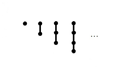
Figure 4. Chain tree ends.

Proof.

By linear algebra, the statement of Lemma 5.6 is equivalent to showing that there are no non-trivial linear relations between point evaluations at different points. Suppose that

(5.10) $$\sum\limits_{k=1}^{n}a_{k}f(x_{k})=0$$

is satisfied for every $f\in E_{1}$, for some $\{a_{k}\}_{1\leq k\leq n}\subseteq\mathbb{R}$. Now define the function $A(\cdot):\mathbb{R}^{2}\rightarrow\mathbb{R}$ as

$$A(\xi):=\sum\limits_{k=1}^{n}a_{k}e^{2\pi i\langle\xi,x_{k}\rangle};$$

$A(\cdot)$ naturally extends to an analytic function $A:\mathbb{C}^{2}\rightarrow\mathbb{C}$. Recalling the standard notation $e(y)=e^{2\pi iy}$, since, by the definition of $E_{1}$, the equality (5.10) holds for every function of the form

(5.11) $$f(x)=\sum\limits_{\begin{subarray}{c}\xi\in\mathcal{S}^{1}\\ \text{finite}\end{subarray}}c_{\xi}e(\langle\xi,x\rangle),$$

for some $\{c_{\xi}\}\subseteq\mathbb{C}$ satisfying $c_{-\xi}=\overline{c_{\xi}}$, by appropriately choosing $f$’s of the form (5.11) we may deduce that $A(\cdot)$ vanishes on the unit circle $\mathcal{S}^{1}\subseteq\mathbb{R}^{2}$.

In what follows we show that $A$ is the zero function on $\mathbb{C}^{2}$, sufficient to yield the statement of Lemma 5.6. First consider the connected curve

$$\mathcal{C}=\{\xi=(\xi_{1},\xi_{2})\in\mathbb{C}^{2}:\xi_{1}^{2}+\xi_{2}^{2}=1\};$$

since the function $A$ is analytic on $\mathbb{C}$ and vanishes on $\mathcal{S}^{1}=\mathcal{C}\cap\mathbb{R}^{2}$, it must vanish on the whole of $\mathcal{C}$. For $1\leq k\leq n$ we write $x_{k}=(b_{k},c_{k})\in\mathbb{R}^{2}$, and with no loss of generality we may assume that all the $b_{k}$ are distinct (otherwise we rotate the plane), and that $\max\limits_{k\leq n}b_{k}=b_{n}$. Now choose $\mu\in\mathbb{R}$, take $\xi=(-i\mu,\sqrt{1+\mu^{2}})\in\mathcal{C}$, and let $\mu\rightarrow\infty$. As, by above, $A(\xi)=0$ on $\mathcal{C}$, we have

$$\begin{split}0&=A(\xi)=\sum\limits_{k=1}^{n}a_{k}e^{2\pi\mu b_{k}}\cdot e(\sqrt{1+\mu}c_{k})\\ &=(1+o_{\mu\rightarrow\infty}(1))a_{n}e^{2\pi\mu b_{n}}e(\sqrt{1+\mu}c_{n}).\end{split}$$

This certainly implies that $a_{n}=0$, and, continuing by induction, we may conclude that all the $a_{k}=0$ must vanish, as claimed above.

∎

To prove Proposition 5.3 we will apply Lemma 5.6. To produce our $h$ (this being the second step below) we perturb a specific function $\phi(x_{1},x_{2})$ in $E_{1}$:

(5.12) $$\phi(x_{1},x_{2})=\sin(\pi x_{1})\cdot\sin(\pi x_{2}).$$

Proof of Proposition 5.3, $n=2$.

For any finite $K\subseteq\mathbb{Z}^{2}$ and

$$\eta:K\rightarrow\{-1,1\}$$

we can find $\psi\in E_{1}$ such that

(5.13) $$\psi(k)=\eta(k)$$

for every $k\in K$. For $\epsilon>0$ sufficiently small the function

(5.14) $$\varphi(x_{1},x_{2})=\varphi_{\phi,\psi;\epsilon}(x_{1},x_{2}):=\phi(x_{1},x_{2})+\epsilon\cdot\psi(x_{1},x_{2}),$$

with $\phi$ given by (5.12) will have its nodal lines in a big compact ball containing $K$ close to those of $\phi$. The manner in which the simple crossing in Figure 3, above, of the nodal lines at each $k\in K$ will resolve for $\epsilon$ small, that is into one of those in Figure 3 below will depend on the sign of $\psi(k)$ (and the sign of $\phi(k)$). In what follows we show that by prescribing the signs of $\psi$ at the cross points it is possible to impose that the function (5.14) attains a given $G\in\mathcal{T}$, for $\epsilon>0$ sufficiently small.

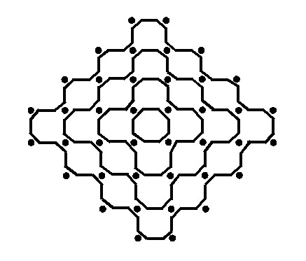
Figure 5. Chain of length $4$ implementation.

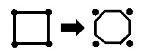
Figure 6. Creating the trivial tree.

More precisely, we prove by induction on $m\geq 1$ the following statement: for every $G\in\mathcal{T}$ with $m$ vertices there exist a finite $K\subseteq\mathbb{Z}^{2}$ and a selection of signs $\{\eta_{k}\}_{k\in K}$, and a compact domain $D\subseteq\mathbb{R}^{2}$, so that prescribing the signs (5.13) for $\psi$ on $K$ yields, for $\epsilon>0$ sufficiently small, a tree end of $\varphi$ (as in (5.14)) restricted to $D$, isomorphic to $G$. First we build any end of the “chain” form, as in Figure 4; that includes the induction basis $m=1$ (the trivial tree as in Figure 6). As it is obvious, this is clearly possible in view of the picture in Figure 5, where our chain is grown with the set of $k$’s involved highlighted.

Now we assume by induction hypothesis that all the tree ends $G\in\mathcal{T}$ with $m<M$ vertices could be attained (in the sense of the induction statement above), and we are going to prove now that the same is true for $G\in\mathcal{T}$ with $M$ vertices. To this end we introduce two operations: engulf and join, that would be instrumental in order for “constructing” $G$ from trees with smaller number of vertices (that is, prescribing the appropriate signs via (5.13), provided that the corresponding signs were readily constructed for smaller trees). These operations are carried out on certain figures connected to finite subsets, $K\subseteq\mathbb{Z}^{2}$ and can be achieved by choosing $\{\eta(k)\}_{k\in K}$ suitably.

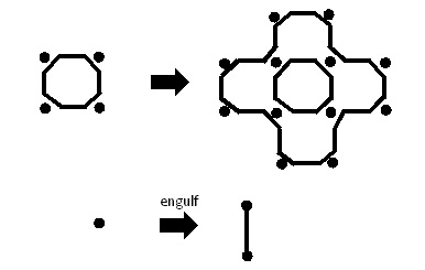
Figure 7. Engulfing a single square (above). The corresponding trees are exhibited below.

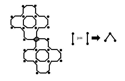
Figure 8. Joining two figures. The corresponding trees are exhibited to the right.

Start with the box of $4$ lattice points (see Figure 6, to the left), which by choosing $\eta(k)$ to be suitable $\pm 1$ at the vertices yields the picture in Figure 6 to the right, represented by a single point in $\mathcal{T}$ (the leftmost tree in Figure 4). Engulf is the operation of enclosing the figure at hand with one new oval. This is done by choosing (uniquely) the squares on the boundary of the figure as indicated in the picture in Figure 7. The join is done by taking two figures, and joining the right lowest corner of one to the left highest corner of the other, as in Figure 8.

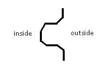
Figure 9. A “kink”. It does not pose a serious problem.

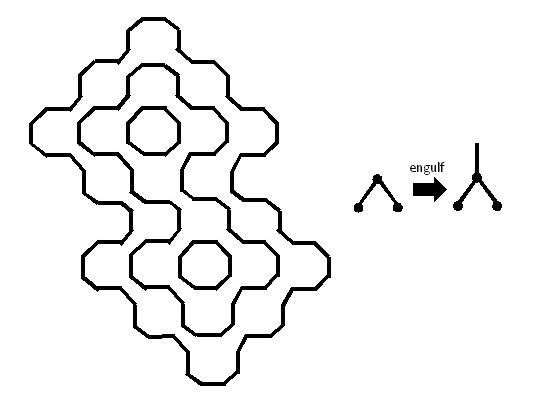
Figure 10. Engulfing a figure with a “kink”.

The figures formed will always have a highest single square at the top and a lowest single square at the bottom, so that there is no ambiguity (this property is true to start off, and is preserved by the two operations). A second point is that engulfing any figure that arises is always possible. The only potential problem is that the join may introduce a non-convex “kink” of the shape, as in Figure 9. This could lead to a block in engulfing. However, as indicated in the example in Figure 10, this does not cause a problem. At any further stage these kinks don’t interact, and one can always engulf.

Let us now formally perform the induction step. Given a tree end $G\in\mathcal{T}$ with $M\geq 2$ vertices, it is either the engulf of a smaller tree ends $G^{\prime}$ (with $M-1$ vertices), or the join of two tree ends $G^{\prime}$ of $M^{\prime}\geq 2$ vertices and $G^{\prime\prime}$ of $M^{\prime\prime}\geq 2$ vertices whence $M=M^{\prime}+M^{\prime\prime}-1$ and we have $M^{\prime},M^{\prime\prime}<M$; denote $\{\eta_{G^{\prime}}(k)\}_{k\in K^{\prime}}$ (resp. $\{\eta_{G^{\prime}}(k)\}_{k\in K^{\prime}}$ and $\{\eta_{G^{\prime\prime}}(k)\}_{k\in K^{\prime\prime}}$) the corresponding signs obtained from the induction hypothesis applied on $G^{\prime}$ (resp. $G^{\prime}$, $G^{\prime\prime}$). Then, by the definition of the engulf (resp. join) procedure we obtain a prescription of the signs $\{\eta_{G}(k)\}_{k\in K}$ on a bigger set $K$ that yields a tree end isomorphic to $G$ on a corresponding domain $D\subseteq\mathbb{R}^{2}$, which concludes the induction step, and therefore also the present proof.

∎

6. Semi-local nodal counts on $\mathcal{M}$

6.1. Local results

Here we formulate a local result (Theorem 6.2 below) around a point $x\in\mathcal{M}$, after blowing up the coordinates according to the natural scaling of

$$f=f_{\alpha;T}:\mathcal{M}\rightarrow\mathbb{R},$$

the band-limited Gaussian functions (1.2). Recall that for $H\in H(n-1)$ (resp. $G\in\mathcal{T}$) Theorem 6.2 yields constants $c_{\mathcal{C};\mathfrak{g_{\alpha}}}(H)$ (resp. $c_{X;\mathfrak{g_{\alpha}}}(G)$) corresponding to the limiting random fields $\mathfrak{g}_{\alpha}$ of $f$, under the same natural scaling around $x$.

Notation 6.1.

1. For $x\in\mathcal{M}$, $r>0$ let $B(x,r)\subseteq\mathcal{M}$ be the geodesic ball in $\mathcal{M}$ of radius $r$.

2. For $H\in H(n-1)$ (resp. $G\in\mathcal{T}$) let

   $$\mathcal{N}_{\mathcal{C}}\left(f_{\alpha;T},H;x,r\right)$$

   (resp. $\mathcal{N}_{X}\left(f_{\alpha;T},G;x,r\right)$) be the number of components of $f_{\alpha;T}^{-1}(0)$ lying in $B(x,r)$ of class $H$ (resp. corresponding to nesting tree isomorphic to $G$).

3. In the situation as above $\mathcal{N}_{\cdot}^{*}(f_{\alpha;T},\cdot;x,r)$ is the number of those merely intersecting $B(x,r)$.

Theorem 6.2 (Cf. [So, Theorem 5]).

For every $H\in H(n-1)$, $G\in\mathcal{T}$, and $x\in\mathcal{M}$ we have

$$\lim\limits_{R\rightarrow\infty}\limsup\limits_{T\rightarrow\infty}\mathcal{P}\left\{\left|\frac{\mathcal{N}_{\mathcal{C}}\left(f_{\alpha;T},H;x,\frac{R}{T}\right)}{\operatorname{Vol}(B(R))}-c_{\mathcal{C};\mathfrak{g_{\alpha}}}(H)\right|>\epsilon\right\}=0,$$

$$\lim\limits_{R\rightarrow\infty}\limsup\limits_{T\rightarrow\infty}\mathcal{P}\left\{\left|\frac{\mathcal{N}_{\mathcal{C}}\left(f_{\alpha;T},G;x,\frac{R}{T}\right)}{\operatorname{Vol}(B(R))}-c_{X;\mathfrak{g_{\alpha}}}(G)\right|>\epsilon\right\}=0.$$

6.2. Proof of Theorem 6.2

Let $f$ be defined as in (1.2). For a fixed point $x\in\mathcal{M}$ we blow up the coordinates around $x$, and consider $f$ on a small geodesic ball $B(x,\epsilon_{0})\subseteq\mathcal{M}$. That is, we define the Gaussian field

$$f_{x;T}(u)=f\left(\exp_{x}(uT^{-1})\right),$$

$u\in T_{x}(\mathcal{M})\cong\mathbb{R}^{n}$ lying a the Euclidian ball

$$u\in B(\epsilon_{0}\cdot T)\subseteq\mathbb{R}^{n}.$$

Since $\mathcal{M}$ is a compact manifold, for $r$ sufficiently small, independent of $x$,

(6.1) $$\mathcal{N}_{\cdot}(f,\cdot;x,r)=\mathcal{N}_{\cdot}(f_{x;T},\cdot;rT),$$

the rhs of the latter equality being of a random field defined on the Euclidian space.

The random field $f_{x;T}$ is Gaussian with covariance kernel

$$\begin{split}K_{x;T}(u,v)&:=\mathbb{E}[f_{x;T}(u)\cdot f_{x;T}(v)]=\mathbb{E}[f(\exp_{x}(uT^{-1}))\cdot f(\exp_{x}(vT^{-1}))]\\ &=K_{\alpha}(T;uT^{-1},vT^{-1}),\end{split}$$

(cf. (1.11)), and (1.12) implies that, as $T\rightarrow\infty$,

(6.2) $$r_{f_{x;T}}(u,v)\approx B_{n,\alpha}(|u-v|)=\mathbb{E}[\mathfrak{g}_{n,\alpha}(u)\cdot\mathfrak{g}_{n,\alpha}(v)].$$

Hence, for every $x\in\mathcal{M}$ fixed, the fields $\{f_{x;T}\}_{T}$, defined on growing domains, converge on $\mathbb{R}^{n}$ to $\mathfrak{g}_{\alpha}$, to be formulated more precisely. In particular, as $f$ and $\mathfrak{g}_{\alpha}$ are defined on different probability spaces, we need to couple them, i.e. define on the same probability space. We now formulate the following proposition that will imply Theorem 6.2 proved immediately after.

Proposition 6.3.

Let $x\in\mathcal{M}$, $R>0$ be sufficiently big, $\delta>0$ be given, $H\in H(n-1)$ and $G\in\mathcal{T}$. Then there exists a coupling of $f$ and $\mathfrak{g}_{\alpha}$ and $T_{0}=T_{0}(R,\delta)$ sufficiently big, so that for all $T>T_{0}$ outside an event of probability $<\delta$ we have

$$\mathcal{N}_{\cdot}(\mathfrak{g}_{\alpha},\cdot;R-1)\leq\mathcal{N}_{\cdot}\left(f,\cdot;x,\frac{R}{T}\right)\leq\mathcal{N}_{\cdot}(\mathfrak{g}_{\alpha},\cdot;R+1).$$

Proposition 6.3 will be proven in §6.3 immediately below.

Proof of Theorem 6.2 assuming Proposition 6.3.

Theorem 6.2 follows from Proposition 6.3 and Theorem 3.3 applied on $\mathfrak{g}_{\alpha}$ at once.

∎

6.3. Some preparatory results towards the proof of Proposition 6.3

The proof of Proposition 6.3 is quite similar to the proof of the analogous statement on nodal count from  [So, Lemmas $6-7$]; here we need to check that the topological and the nesting nodal structure rather than merely the nodal count is stable under the perturbation. In order to prove Proposition 6.3 we need to excise the following exceptional events $\Delta_{i}$, $1\leq i\leq 4$.

Let $\delta>0$ be a small parameter that will control the probabilities of the discarded events, $\beta>0$ a small parameter that will control the quality of the various approximations, and $M>0$ a large parameter. Given $R$ and $T$ big we define

$$\Delta_{1}=\Delta_{1}(R,T;\beta)=\{\|f_{x;T}-\mathfrak{g}_{\alpha}\|_{C^{1}(\overline{B}(2R))}\geq\beta\},$$

$$\Delta_{2}=\Delta_{2}(R,T;\delta,M)=\left\{\|f_{x;T}\|_{C^{2}(\overline{B}(2R))}\geq\delta^{-1}M\right\},$$

$$\Delta_{3}=\Delta_{3}(R;\delta,M)=\left\{\|\mathfrak{g}_{\alpha}\|_{C^{2}(\overline{B}(2R))}\geq\delta^{-1}M\right\}$$

and the “unstable event”

$$\Delta_{4}(R,T;\beta)=\left\{\min\limits_{u\in\overline{B}(2R)}\max\{|f_{x;T}(u)|,|\nabla f_{x;T}(u)|\}\leq 2\beta\right\}.$$

The following lemma from  [So] is instrumental in proving that for $f$ and $\mathfrak{g}_{\alpha}$ suitably coupled the exceptional events have small probability. Recall that we have (6.2); more precisely (1.12) implies that the covariance function of $f_{x;T}$ together with its derivatives converge uniformly to the covariance function of $\mathfrak{g}_{\alpha}$ and its respective derivatives.

Lemma 6.4 ([So, Lemma $4$]).

Given $x\in\mathcal{M}$, $R>0$ and $\upsilon>0$ there exists a coupling of $f$ and $\mathfrak{g}_{\alpha}$ and $T_{0}=T_{0}(R,\upsilon)$ with

$$\mathbb{E}\left[\|f_{x;T}-\mathfrak{g}_{\alpha}\|_{C^{1}(\overline{B}(2R))}\right]<\upsilon$$

for all $T\geq T_{0}$.

From this point we will avoid mentioning coupling that will be understood implicitly. The following is a simple corollary from Lemma 6.4.

Lemma 6.5.

For $R>0$ sufficiently big given, and $\beta,\delta>0$ there exists $T_{0}=T_{0}(R,\beta,\delta)$ so that for $T>T_{0}$ the probability of $\Delta_{1}$ is

(6.3) $$\mathcal{P}(\Delta_{1}(R,T;\beta))<\delta$$

arbitrarily small.

The following lemma yields a bound on the probability $\mathcal{P}(\Delta_{2})$ and $\mathcal{P}(\Delta_{3})$.

Lemma 6.6.

1. For every $R>0$ sufficiently big there exists $M=M(R)>0$ so that for all $\delta>0$

   (6.4) $$\mathcal{P}(\Delta_{3}(R;\delta,M))<\delta.$$

2. For $R>0$ there exists $M(R)>0$ and $T_{0}=T_{0}(R)$ so that for all $T>T_{0}$ and $\delta>0$

   (6.5) $$\mathcal{P}(\Delta_{2}(R,T;\delta,M))<\delta.$$

Proof.

For (6.4) we may choose $M$ to be

$$M=\mathbb{E}[\|\mathfrak{g}_{\alpha}\|_{C^{2}(\overline{B}(2R))}]<\infty,$$

finite by [A-T], Theorem $2.1.1$. The estimate (6.4) with $M$ as here then follows by Chebyshev’s inequality.

In order to establish (6.5) we observe that by [A-T], Theorem $2.2.3$ (“Sudakov-Fernique comparison inequality”) and (1.12) applied to both $K_{x;T}$ and its derivatives for all $M_{1}>M$ there exists $T_{0}=T_{0}(R,M_{1})$ such that for all $T>T_{0}$

$$\mathbb{E}\left[\|f_{x;T}\|_{C^{2}(\overline{B}(2R))}\right]<M_{1}.$$

Hence (6.5) follows from using Chebyshev’s inequality as before. Using $M_{1}$ instead of $M$ will also work with (6.4).

∎

Finally, for the unstable event $\Delta_{4}$ we have the following bound:

Lemma 6.7 ([So, Lemma $5$]).

For $R>0$ sufficiently big given, $M>0$ and $\delta>0$ there exist $\beta=\beta(R,M,\delta)>0$ and $T_{0}=T_{0}(R,M,\delta)>0$ so that for all $T>T_{0}$ outside $\Delta_{2}\cup\Delta_{3}$ the probability of $\Delta_{4}$ is

(6.6) $$\mathcal{P}\left(\Delta_{4}(R,T;\beta)\setminus(\Delta_{2}(R,T;\delta,M)\cup\Delta_{3}(R;\delta,M))\right)<\delta$$

arbitrarily small.

6.4. Proof of Proposition 6.3

Proposition 6.8 (cf. [So, Lemma $6$]).

Outside of $\Delta_{1}\cup\Delta_{4}$ we have

$$\mathcal{N}_{\cdot}(\mathfrak{g}_{\alpha},\cdot;R-1)\leq\mathcal{N}_{\cdot}\left(f_{x;T},\cdot;R\right)\leq\mathcal{N}_{\cdot}(\mathfrak{g}_{\alpha},\cdot;R+1).$$

Proof of Proposition 6.3 assuming Proposition 6.8.

Since the probability of the
events $\Delta_{i}$, $i=1\ldots 4$ is $<4\delta$ for $T>T_{0}(R,\beta,\delta)$ by lemmas 6.5-6.7, the statement of Proposition 6.3 follows from Proposition 6.8 at once upon replacing $\delta$ by $\frac{\delta}{4}$, bearing in mind (6.1).

∎

Proof of Proposition 6.8.

Modifying the proofs of [So, Lemmas $6,7$], here we only prove the somewhat more complicated case of tree ends: outside of $\Delta_{1}\cup\Delta_{4}$ for $G\in\mathcal{T}$ one has

(6.7) $$\mathcal{N}_{X}(\mathfrak{g}_{\alpha},G;R-1)\leq\mathcal{N}_{X}(f_{x;T},G;R),$$

with the inequality

$$\mathcal{N}_{X}\left(f_{x;T},G;R\right)\leq\mathcal{N}_{X}(\mathfrak{g}_{\alpha},G;R+1),$$

and their analogues for nodal components topology following along the same lines. Outside $\Delta_{1}\cup\Delta_{4}$ we have

(6.8) $$\|f_{x;T}-\mathfrak{g}_{\alpha}\|_{C^{1}(\overline{B}(2R))}<\beta,$$

and also

(6.9) $$\min\limits_{\overline{B}(2R)}\max\{|f_{x;T}|,|\nabla f_{x;T}|\}>\beta;\;\min\limits_{\overline{B}(2R)}\max\{|\mathfrak{g}_{\alpha}|,|\nabla\mathfrak{g}_{\alpha}|\}>\beta.$$

For $t\in[0,\beta]$ consider

$$g_{t}:=\mathfrak{g}_{\alpha}+\frac{t}{\beta}\cdot(f_{x;T}-\mathfrak{g}_{\alpha}).$$

We claim that for all $t\in[0,\beta]$, $g_{t}$ has no critical zeros in $B(2R)$, i.e. points $y\in B(2R)$ such that $g_{t}(y)=0$ and $\nabla g_{t}(y)=0$. Otherwise let $t_{0}\in[0,\beta]$ and $y_{0}\in B(2R)$ such that $g_{t_{0}}(y_{0})=0$, $\nabla g_{t_{0}}(y_{0})=0$. This contradicts (6.9), as then

$$|\mathfrak{g}_{\alpha}(y_{0})|=\left|g_{t_{0}}(y_{0})-\frac{t_{0}}{\beta}\cdot(f_{x;T}(y_{0})-\mathfrak{g}_{\alpha}(y_{0}))\right|=\frac{t_{0}}{\beta}|f_{x;T}(y_{0})-\mathfrak{g}_{\alpha}(y_{0})|<\beta$$

by (6.8), and

$$\begin{split}|\nabla\mathfrak{g}_{\alpha}(y_{0})|&=\left|\nabla g_{t_{0}}(y_{0})-\frac{t_{0}}{\beta}\cdot\nabla(f_{x;T}-\mathfrak{g}_{\alpha})(y_{0})\right|\\ &=\frac{t_{0}}{\beta}\cdot|\nabla(f_{x;T}-\mathfrak{g}_{\alpha})(y_{0})|<\beta,\end{split}$$

again, by (6.8). That concludes the proof of the non-existence of critical zeros of $g_{t}$, $t\in[0,\beta]$ in $B(2R)$.

Now, since under the assumptions of Proposition 6.8, we excluded the event $\Delta_{1}\cup\Delta_{4}$, that implies that the various components $\gamma$ of $\mathfrak{g}_{\alpha}^{-1}(0)$ are regular and bounded away from each other. Moreover Nazarov-Sodin [So, Lemmas $6,7$] showed that each component $\gamma$ lies in an “annulus” inside

$$\gamma_{1}=\{y\in\mathbb{R}^{n}:d(y,\gamma)<1\},$$

bounded by the two hypersurfaces $\mathfrak{g}_{\alpha}(x)=\pm\beta$, where $\beta>0$ is assumed to be sufficiently small; different components $\gamma$ correspond to different, pairwise disjoint annuli.

Since $\Delta_{1}$ was excluded, for every $t\in[0,\beta]$, $g_{t}(y)>0$ is positive on $\mathfrak{g}_{\alpha}^{-1}(\beta)$ and $g_{t}(y)<0$ is negative on $\mathfrak{g}_{\alpha}^{-1}(-\beta)$. Therefore for every $\gamma$ component of $\mathfrak{g}_{\alpha}$ lying in $B(R)$ and $t\in[0,\beta]$, $g_{t}^{-1}(0)$ contains at least one component lying in $\gamma_{1}$. A standard result from the Differential Topology asserts that a $1$-parameter family $g_{t}:\gamma_{1}\rightarrow\mathbb{R}$, $t\in[0,\beta]$ defined on the open bounded annulus $\gamma_{1}$, so that for all $t\in[0,a]$, the function $g_{t}$ admits no non-degenerate critical points (i.e. it is a Morse function), the zero sets $\{g_{t}^{-1}(0)\}$ are diffeomorphic; note that, by the above, there is no nodal intersection with the boundary $\partial\gamma_{1}$, as here $g_{t}$ is strictly positive or negative.

By the above, for every $\gamma$ component of $\mathfrak{g}_{\alpha}^{-1}(0)$ lying in $B(R)$ and $t\in[0,\beta]$ there exists a unique component $\gamma^{t}$ of $g_{t}^{-1}(0)$ lying in $\gamma_{1}\subseteq B(R+1)$ (by the above, components cannot merge or split in $\gamma_{1}$; new components would also generate a critical point). In particular, the correspondence $\gamma\mapsto\gamma^{t}$ is well-defined and injective between components of $\mathfrak{g}_{\alpha}^{-1}(0)$ lying in $B(R)$ and the components of $g_{t}^{-1}(0)$ lying in $B(R+1)$, and moreover $\gamma$ and $\gamma^{t}$ are diffeomorphic.

Furthermore, the nesting tree of $g_{t}$ is preserved: there exists an injective map $\phi^{t}:\Omega_{0}\rightarrow\Omega_{t}$ between the vertices of the nesting trees of $g_{0}=\mathfrak{g}_{\alpha}$ and $g_{t}$ respectively such that $\omega,\omega^{\prime}\in\Omega_{0}$ are connected by an oval $\gamma$ of $\mathfrak{g}_{\alpha}^{-1}(0)$, if and only if $\phi^{t}(\omega),\phi^{t}(\omega^{\prime})\in\Omega_{t}$ are connected by the oval $\gamma^{t}$ of $g_{t}^{-1}(0)$. Equivalently, if $\omega$ is the domain lying inside $\gamma_{1}$ and outside $\gamma_{2}$, then $\phi^{t}(\omega)$ is the domain lying inside $\gamma_{1}^{t}$ and outside $\gamma_{2}^{t}$ (by Jordan’s Theorem in this setting, see section 2). No new ovals are created inside ovals corresponding to $\gamma\subseteq B(R-1)$, as otherwise there would exist critical zeros, that were already ruled out.

Now let $c\in\mathcal{C}(\mathfrak{g}_{\alpha})$ be a nodal component of $\mathfrak{g}_{\alpha}$ lying in $B(R-1)$, with $e(c)$ isomorphic a given rooted tree $G$. By the above, for every $t\in[0,\beta]$ the nesting tree end $e_{g_{t}^{-1}(0)}(c^{t})$ is isomorphic to $e(c)$, and hence to $G$. As

$$c^{t}\subseteq\{y:d(y,c)\leq 1\}\subseteq B(R),$$

it implies (6.7) as claimed. ∎

7. Proof of Theorem 1.1: gluing local results on $\mathcal{M}$

7.1. Proof of Theorem 1.1

In this section we finally prove Theorem 1.1 with the measures

(7.1) $$\mu_{\mathcal{C},n,\alpha}=\mu_{\mathcal{C}(\mathfrak{g}_{\alpha})}$$

and

(7.2) $$\mu_{X,n,\alpha}=\mu_{X(\mathfrak{g}_{\alpha})},$$

as in Notation 4.1; both $\mu_{\mathcal{C}(\mathfrak{g}_{\alpha})}$ and $\mu_{X(\mathfrak{g}_{\alpha})}$ are probability measures by the virtue of Theorem 4.2, parts (2) and (3) respectively. First we formulate the following theorem that will imply Theorem 1.1 at once; for $H\in H(n-1)$ (resp. $G\in\mathcal{T}$) let $\mathcal{N}_{\mathcal{C}}(f,H)$ (resp. $\mathcal{N}_{X}(f,H)$) the the total number of components $c\in\mathcal{C}(f)$ of topological class $H$ (resp. such that $e(c)$ isomorphic to $G$).

Theorem 7.1.

For every $H\in H(n-1)$, $G\in\mathcal{T}$ we have

$$\mathbb{E}\left[\left|\frac{\mathcal{N}_{\mathcal{C}}(f,H)}{T^{n}}-\operatorname{Vol}\mathcal{M}\cdot c_{\mathcal{C};\mathfrak{g}_{\alpha}}(H)\right|\right]\rightarrow 0$$

and

$$\mathbb{E}\left[\left|\frac{\mathcal{N}_{X}(f,G)}{T^{n}}-\operatorname{Vol}\mathcal{M}\cdot c_{X;\mathfrak{g}_{\alpha}}(G)\right|\right]\rightarrow 0.$$

Proof of Theorem 1.1 assuming Theorem 7.1.

As it was mentioned above we take the postulated limiting measures $\mu_{\mathcal{C},n,\alpha}$ and $\mu_{X,n,\alpha}$ to be given by (7.1) and (7.2) respectively. As these are probability measures having the full support $H(n-1)$ and $\mathcal{T}$ respectively by the virtue of theorems 4.2 and 5.1, the only thing remaining to be proven is (1.8).

Here we only prove (1.8) for $\mu_{\mathcal{C}}$, i.e. that for all $\epsilon>0$

(7.3) $$\mathcal{P}\left\{f\in\mathcal{E}_{\mathcal{M},\alpha}(T):\>D(\mu_{\mathcal{C}(f)},\mu_{\mathcal{C},n,\alpha})>\epsilon\right\}\rightarrow 0,$$

the proof for $\mu_{X(f)}$ being identical. Let $\epsilon>0$ be given. Bearing in mind the definition (4.3) of $\mu_{\mathcal{C},n,\alpha}=\mu_{\mathcal{C}(\mathfrak{g}_{\alpha})}$ and (3.2), Theorem 7.1 implies that for every $H\in H(n-1)$ we have

(7.4) $$\mathcal{P}\left\{\left|\mu_{\mathcal{C}(f)}(H)-\mu_{\mathcal{C},n,\alpha}(H)\right|>\epsilon\right\}\rightarrow 0,$$

as $T\rightarrow\infty$. Let

$$H(n-1)=\{H_{k}\}_{k\geq 1}$$

be any enumeration of the (countable) family $H(n-1)$ of $(n-1)$-dimensional topological classes embeddable in $\mathcal{S}^{n}$ (equivalently, embeddable in $\mathbb{R}^{n}$), and for $K\geq 1$ let

$$H(n-1;K)=\{H_{k}:k\leq K\}.$$

Now, since $\mu_{\mathcal{C},n,\alpha}$ is a probability measure, there exists $K=K(\epsilon)$ sufficiently big so that

(7.5) $$\mu_{\mathcal{C},n,\alpha}(H(n-1)\setminus H(n-1;K))<\frac{\epsilon}{4}.$$

For every $\delta>0$ and

$$H_{k}\in H(n-1;K)$$

we employ (7.4) with $\epsilon$ replaced by $\epsilon/2K$ to obtain

$$\widetilde{T_{0}}(H_{k})=\widetilde{T_{0}}(H_{k},K,\epsilon,\delta)$$

such that

(7.6) $$\mathcal{P}\left\{\left|\mu_{\mathcal{C}(f)}(H)-\mu_{\mathcal{C},n,\alpha}(H)\right|>\frac{\epsilon}{4K}\right\}<\frac{\delta}{2K}.$$

Let

$$T_{0}=T_{0}(\epsilon,\delta)=\max\limits_{k\leq K}\widetilde{T_{0}}(H_{k}),$$

and

$$C\subseteq H(n-1;K)$$

a sub-collection of topology classes. Summing up (7.6) for $H_{k}\in C$ and on using the triangle inequality we obtain

(7.7) $$\mathcal{P}\left\{\left|\mu_{\mathcal{C}(f)}(C)-\mu_{\mathcal{C},n,\alpha}(C)\right|>\frac{\epsilon}{4}\right\}<\frac{\delta}{2}$$

holding for every $T>T_{0}$, with the exceptional event of probability $<\frac{\delta}{2}$ independent of $C$. In particular, for $C=H(n-1,K)$, (7.7) is

(7.8) $$\mathcal{P}\left\{\left|\mu_{\mathcal{C}(f)}(H(n-1,K))-\mu_{\mathcal{C},n,\alpha}(H(n-1,K))\right|>\frac{\epsilon}{4}\right\}<\frac{\delta}{2},$$

and since both $\mu_{\mathcal{C}(f)}$ and $\mu_{\mathcal{C},n,\alpha}$ are probability measures, by taking the complement

$$H(n-1)\setminus H(n-1;K),$$

(7.8) is equivalent to

(7.9) $$\begin{split}\mathcal{P}\bigg{\{}\bigg{|}&\mu_{\mathcal{C}(f)}(H(n-1)\setminus H(n-1;K))\\ &-\mu_{\mathcal{C},n,\alpha}(H(n-1)\setminus H(n-1;K))\bigg{|}>\frac{\epsilon}{4}\bigg{\}}<\frac{\delta}{2}.\end{split}$$

Taking into account (7.5), (7.8) implies that

(7.10) $$\mathcal{P}\left\{\mu_{\mathcal{C}(f)}(H(n-1)\setminus H(n-1;K))>\frac{\epsilon}{2}\right\}<\frac{\delta}{2}.$$

In light of all the above we may use (7.7), (7.10) and (7.5) to finally write for every

$$A\subseteq H(n-1)$$

and $T>T_{0}(\epsilon,\delta)$,

(7.11) $$\begin{split}\mathcal{P}\big{\{}\big{|}\mu_{\mathcal{C}(f)}(A)-&\mu_{\mathcal{C},n,\alpha}(A)\big{|}>\epsilon\big{\}}\leq\\ \leq\mathcal{P}\big{\{}\big{|}\mu_{\mathcal{C}(f)}&(A\cap H(n-1;K))-\mu_{\mathcal{C},n,\alpha}(A\cap H(n-1;K))\big{|}>\epsilon/4\big{\}}\\ +\mathcal{P}\big{\{}&\mu_{\mathcal{C}(f)}(A\setminus H(n-1;K))>\epsilon/2\big{\}}<\frac{\delta}{2}+\frac{\delta}{2}=\delta,\end{split}$$

where the exceptional event of probability $<\delta$ independent of $A$. Since $\delta>0$ was arbitrary, and $T_{0}$ is independent of $A$, recalling the definition (1.5) of the distance $D(\cdot,\cdot)$ between probability measures on $H(n-1)$, (7.11) implies the convergence result claimed in (7.3), which, as it was mentioned above, was the only thing missing detail for completing the proof of Theorem 1.1.

∎

7.2. Proof of Theorem 7.1

Proof.

We write the absolute value as

$$|\cdot|=|\cdot|_{+}+|\cdot|_{-}$$

with $|b|_{+}=\max(b,0)$ and $|b|_{-}=\max(-b,0)$. To prove Theorem 7.1 it is then sufficient to bound each of

$$\mathbb{E}\left[\left|\frac{\mathcal{N}_{\cdot}(f,\cdot)}{T^{n}}-\operatorname{Vol}\mathcal{M}\cdot c_{\cdot;\mathfrak{g}_{\alpha}}(\cdot)\right|_{\pm}\right].$$

The latter is the content of Proposition 7.2 to follow immediately. ∎

Proposition 7.2.

For every $H\in H(n-1)$ and $G\in\mathcal{T}$

(7.12) $$\mathbb{E}\left[\left|\frac{\mathcal{N}_{\cdot}(f,\cdot)}{T^{n}}-\operatorname{Vol}\mathcal{M}\cdot c_{\cdot;\mathfrak{g}_{\alpha}}(\cdot)\right|_{\pm}\right]\rightarrow 0.$$

Proposition 7.2 will be proved in §7.4, only in the (most subtle) case

(7.13) $$\mathbb{E}\left[\left|\frac{\mathcal{N}_{\cdot}(f,\cdot)}{T^{n}}-\operatorname{Vol}\mathcal{M}\cdot c_{X;\mathfrak{g}_{\alpha}}(G)\right|_{+}\right]\rightarrow 0.$$

the other $3$ cases (choosing $X$ or $\mathcal{T}$, $|\cdot|_{+}$ or $|\cdot|_{-}$) being proved along similar (but somewhat easier) lines.

7.3. Some preparatory lemmas towards the proof of Proposition 7.2

7.3.1. Excising very small and very long domains

Definition 7.3.

Let $\xi,D>0$ be parameters.

1. A component $c\in\mathcal{C}(f)$ is $\xi$-small if it is a boundary of a nodal domain whose volume in $\mathcal{M}$ is $<\xi T^{-n}$. Let $\mathcal{N}_{\mathcal{C};\xi-sm}(f)$ be the total number of $\xi$-small components of $f$ on $\mathcal{M}$.

2. For $D>0$ a nodal component $c\in\mathcal{C}(f)$ is $D$-long if its diameter is $>D/T$. Let $\mathcal{N}_{\mathcal{C};D-long}(f)$ be their total number.

3. Given parameters $D,\xi>0$ a nodal component $c\in\mathcal{C}(f)$ is ($D,\xi$)-normal, if it is not $\xi$-small nor $D$-long.

4. For $G\in\mathcal{T}$ let $\mathcal{N}_{X;norm}(f,G)$ be the total number of $(\xi,D)$-normal components $c\in\mathcal{C}(f)$ of $f$ such that $e(c)$ is isomorphic to $G$.

5. For $x\in\mathcal{M}$, $r>0$ let $\mathcal{N}_{X;norm}(f,G;x,r)$ (resp. $\mathcal{N}_{X;norm}^{*}(f,G;x,r)$) be the number of those $c$ contained in the geodesic ball $B(x,r)\subseteq\mathcal{M}$ (resp. intersecting $\overline{{B}(x,r)}$). (Here we use Jordan’s Theorem on the sphere to choose those vertices of $e(c)$ lying inside $B(x,r)$, or intersect it respectively).

By the definition of normal ovals, we have

(7.14) $$\mathcal{N}_{X;norm}^{*}(f,G;x,r)\leq\mathcal{N}_{X;norm}\left(f,G;x,r+\frac{D}{T}\right)$$

(as we discarded the very long ovals), and uniformly

(7.15) $$\mathcal{N}_{X;norm}(f,G;x,r)\leq\xi^{-1}T^{n}\operatorname{Vol}_{\mathcal{M}}B(x,r),$$

by a volume estimate (as we discarded the very small domains).

Lemma 7.4 (Cf. [So, Lemma $8$]).

There exists a constant $C_{0}>0$ such that the following bound holds for the number of $D$-long components:

$$\limsup\limits_{T\rightarrow\infty}\frac{\mathbb{E}[\mathcal{N}_{\mathcal{C};D-long}(f)]}{T^{n}}\leq C_{0}\cdot\frac{1}{D}$$

A proof, given in this generality in  [So] and omitted here, is by taking a $D/T$-net on $\mathcal{M}$ and using the Kac-Rice estimate (2.8).

Lemma 7.5 (Cf. [So, Lemma $9$], and Lemma 4.12 in the scale-invariant case).

Then there exist constants $c_{0},C_{0}>0$ so that the following estimate on the number of $\xi$-small components:

$$\limsup\limits_{T\rightarrow\infty}\frac{\mathbb{E}[\mathcal{N}_{\mathcal{C};\xi-sm}(f)]}{T^{n}}\leq C_{0}\cdot\xi^{c_{0}}.$$

The proof of Lemma 7.5, omitted here, is very similar to the proof of Lemma 4.12, given in §4.6 of the present manuscript.

7.3.2. Integral geometric sandwich on $\mathcal{M}$ for normal components

Lemma 7.6 (Integral-geometric sandwich on a Riemannian manifold, cf. [So, Lemma $1$], and Lemma 3.7 in the scale-invariant case).

Let $G\in\mathcal{T}$. Given $\epsilon>0$, there exists $\eta>0$ such that for every $r<\eta$,

(7.16) $$\begin{split}\mathcal{N}_{X;norm}(f,G)&\leq(1+\epsilon)\int\limits_{\mathcal{M}}\frac{\mathcal{N}_{X;norm}^{*}(f,G;x,r)}{\operatorname{Vol}(B(r))}dx\\ &+\xi^{-1}T^{n}\operatorname{Vol}_{\mathcal{M}}(B_{x}(r))+O_{G}(1).\end{split}$$

The proof of Lemma 7.6 is very similar to the one of Lemma 3.7, and we omit it here.

Remark 7.7.

1. Note the differences between (7.16) and the analogous statement (3.5) in the scale invariant case. First, the $(1+\epsilon)$ factor in (7.16) manifests the perturbed volumes of small geodesic balls on $\mathcal{M}$ as compared to the Euclidian balls. We then need to account for a (exclusive to $\mathcal{N}_{X}$) situation where a component $c\in\mathcal{C}(f_{L})$ is contained in some geodesic ball $B_{x}(r)$, but the corresponding tree end is not, which may be bounded by the volume estimate (7.15) responsible for the first extra term in (7.16). The other peculiar $O_{G}(1)$ term in (7.16) may be taken as at most the vertex number of $G$.

2. For the lower bound the following inequality holds outside an event of arbitrarily small probability only (The reason that this may not always hold is again, that in the non-Euclidean case the graph end $e(c)$ may fail to be lying in a geodesic ball, even if $c$ is)

   $$(1-\epsilon)\int\limits_{\mathcal{M}}\frac{\mathcal{N}_{X;norm}(f,G;x,r)}{\operatorname{Vol}(B(r))}dx\leq\mathcal{N}_{X;norm}(f,G).$$

7.3.3. Uniform bound for the number of components in small balls

Lemma 7.8.

For $r$ sufficiently small, depending only on $\mathcal{M}$ we have the following uniform bound

$$\mathbb{E}[\mathcal{N}_{\mathcal{C}}(f;x,r)]=O(r^{n}\cdot T^{n}),$$

with constant involved in the $`O^{\prime}$-notation depending on $\mathcal{M}$ only.

Proof.

First, the nodal components count is bounded

$$\mathcal{C}(f)\leq\mathbb{E}[\mathcal{A}(f)]$$

by the number of critical points of $f$. To bound the latter we use Lemma 2.2 on

$$G=\nabla f,$$

understood in a coordinate patch around $x$. We claim that (1.12), applied on $K_{\alpha}(T;x,y)$ and its derivatives, implies that the expression

(7.17) $$\frac{\mathbb{E}[|\nabla G(x)|^{2}]^{n/2}}{\left(\det\mathbb{E}[G(x)\cdot G(x)^{t}]\right)^{1/2}}=\frac{\mathbb{E}[|(f_{ij}(x))_{i,j}|^{2}]^{n/2}}{\left(\det\mathbb{E}[\nabla f(x)\cdot\nabla f(x)^{t}]\right)^{1/2}}=O(T^{n}),$$

on the rhs of (2.8) is uniformly bounded, with constant involved in the $`O^{\prime}$-notation depending only on $n$.

First, we observe that the denominator of (7.17) is the determinant of the covariance matrix $\Sigma(x)$ of $\nabla f(x)$. We know from (1.12) that, after scaling by $T$, the entries of $\Sigma(x)$ converge uniformly to the entries of the non-degenerate covariance matrix of $\nabla\mathfrak{g}$. Hence, properly scaled,

$$\det\mathbb{E}[\nabla f(x)\cdot\nabla f(x)^{t}]$$

is bounded away from $0$. Concerning the numerator $\mathbb{E}[|f_{ij}(x)|]$ of (7.17), we may use the triangle inequality to bound

$$\mathbb{E}[|(f_{ij}(x))|^{2}]\leq\sum\limits_{i,j}\mathbb{E}\left[f_{ij}(x)^{2}\right];$$

after scaling by $T$ (consistent with the scaling of the denominator), the latter is uniformly bounded, due to (1.12) applied to the corresponding $4$-th order mixed derivative. Hence (2.8) implies the statement of the present lemma.

∎

7.4. Proof of Proposition 7.2

Proof.

Throughout the course of this proof we will assume with no loss of generality that $\mathcal{M}$ is unit volume $\operatorname{Vol}\mathcal{M}=1$, and for a given $G\in\mathcal{T}$ we will use the shorthand

(7.18) $$c_{X}:=c_{X;\mathfrak{g}_{\alpha}}(G);$$

and as it was mentioned above we only show (7.13) here. Let $R>0$ be a large number, so that $D/R$ is sufficiently small, and $R/T<\eta$ as in Lemma 7.6, sufficiently small, so that

(7.19) $$\begin{split}&\left|\frac{\operatorname{Vol}_{\mathcal{M}}(B_{x}(R/T))}{\operatorname{Vol}(B(R/T))}-1\right|<\epsilon,\\ &\frac{\operatorname{Vol}(B(R+D))}{\operatorname{Vol}(B(R))}<1+\epsilon\end{split}$$

uniformly for $x\in\mathcal{M}$.

Apply Lemma 7.6 with $r=\frac{R}{T}$; by the triangle inequality for $|\cdot|_{+}$ we have (recall (7.18))

(7.20) $$\begin{split}&\mathbb{E}\left[\left|\frac{\mathcal{N}_{\mathcal{T};norm}(f,G)}{T^{n}}-\operatorname{Vol}\mathcal{M}\cdot c_{X}\right|_{+}\right]\\ &\leq\mathbb{E}\left[\int\limits_{\mathcal{M}}\left|(1+2\epsilon)\frac{\mathcal{N}_{X;norm}^{*}(f,G;x,R/T)}{\operatorname{Vol}B(R+D)}-c_{X}\right|_{+}dx\right]\\ &+O(T^{-n}+\xi^{-1}\operatorname{Vol}_{\mathcal{M}}(B_{x}(R/T)))\\ &\leq\mathbb{E}\left[\int\limits_{\mathcal{M}}\left|\frac{\mathcal{N}_{X;norm}(f,G;x,(R+D)/T)}{\operatorname{Vol}B(R+D)}-c_{X}\right|_{+}dx\right]\\ &+O\left(\epsilon\cdot\int\limits_{\mathcal{M}}\frac{\mathbb{E}[\mathcal{N}_{X;norm}(f,G;x,(R+D)/T)]}{\operatorname{Vol}B(R+D)}dx\right)\\ &+O(T^{-n}+\xi^{-1}\operatorname{Vol}_{\mathcal{M}}(B_{x}(R/T))),\end{split}$$

by (7.14) and (7.19). Observe that the integrand

$$\frac{\mathbb{E}[\mathcal{N}_{X;norm}(f,G;x,(R+D)/T)]}{\operatorname{Vol}B(R+D)}$$

is uniformly bounded by Lemma 7.8. Hence (7.20) is

$$\begin{split}&\mathbb{E}\left[\left|\frac{\mathcal{N}_{X;norm}(f,G)}{T^{n}}-\operatorname{Vol}\mathcal{M}\cdot c_{X}\right|_{+}\right]\\ &\leq\mathbb{E}\left[\int\limits_{\mathcal{M}}\left|\frac{\mathcal{N}_{X;norm}(f,G;x,(R+D)/T)}{\operatorname{Vol}B(R+D)}-c_{X}\right|_{+}dx\right]\\ &+O(\epsilon+T^{-n}+\xi^{-1}\operatorname{Vol}_{\mathcal{M}}(B_{x}(R/T))),\end{split}$$

Since the latter error term $O(\cdots)$ could be made arbitrarily small, it is then sufficient to prove that

(7.21) $$\begin{split}&\mathbb{E}\left[\int\limits_{\mathcal{M}}\left|\frac{\mathcal{N}_{X;norm}(f,G;x,(R+D)/T)}{\operatorname{Vol}B(R+D)}-c_{X}(G,x)\right|_{+}dx\right]\\ &=\int\limits_{\Delta}\int\limits_{\mathcal{M}}\left|\frac{\mathcal{N}_{X;norm}(f,G;x,(R+D)/T)}{\operatorname{Vol}B(R+D)}-c_{X}\right|_{+}dxd\mathcal{P}(\omega)\rightarrow 0,\end{split}$$

where $\Delta$ is the underlying probability space, and $\mathcal{P}$ is the probability measure on $\Delta$. Now consider the event

$$\Delta_{T,G;x,R}=\left\{\left|\frac{\mathcal{N}_{X}(f,G;x,R/T)}{\operatorname{Vol}B(R+D)}-c_{X}\right|>\epsilon\right\};$$

note that though formally the values of $T$ can attain a continuum variety in $\mathbb{R}$, only countably many of them would yield genuinely different functions $f$ in (1.2) and their by-products, such as $\Delta_{T,G;x,R}$, so we may assume that any limit $T\rightarrow\infty$ is along this countable system; from this point on we will neglect this difference, which will save us from dealing with various measurability issues. Then by Theorem 6.2, for every $x\in\mathcal{M}$

(7.22) $$\lim\limits_{R\rightarrow\infty}\limsup\limits_{T\rightarrow\infty}\mathcal{P}(\Delta_{T,G;x,R+D})=0.$$

We claim that there exists a sequence $\{R_{j}\}_{j\rightarrow\infty}$ (e.g. $R_{j}\in\mathbb{Z}$ integers) so that the limit (7.22) is almost uniform w.r.t. $x\in X$, that is, for every $\eta>0$ there exists $\mathcal{M}_{\eta}\subseteq\mathcal{M}$ with $\operatorname{Vol}\mathcal{M}_{\eta}>1-\eta$, such that

(7.23) $$\varliminf\limits_{R_{j}\rightarrow\infty}\varlimsup\limits_{T\rightarrow\infty}\sup\limits_{x\in\mathcal{M}_{\eta}}\mathcal{P}(\Delta_{T,G;x,R_{j}+D})=0.$$

To see (7.23) we first apply an Egorov-type theorem on the limit in (7.22) w.r.t. $R\rightarrow\infty$: working with the sets

$$E_{n,k}=\bigcup\limits_{R>n\text{ integer}}\left\{x\in\mathcal{M}:\>\mathcal{P}(\Delta_{T,G;x,R+D})>\frac{1}{k}\text{ for }T\text{ sufficiently big}\right\}$$

yields that for some $\mathcal{M}_{\eta}$ with $\operatorname{Vol}(\mathcal{M}_{\eta})>1-\frac{\eta}{2}$

$$\lim\limits_{R_{j}\rightarrow\infty}\sup\limits_{x\in\mathcal{M}_{\eta}}\varlimsup\limits_{T\rightarrow\infty}\mathcal{P}(\Delta_{T,G;x,R_{j}+D})=0;$$

this is not quite the same as the claimed result (7.23), as the order of $\sup\limits_{x\in\mathcal{M}_{\eta}}$ and the $\limsup$ w.r.t. $T\rightarrow\infty$ is wrong. We use an Egorov-type argument once again, w.r.t. the limit $\varlimsup\limits_{T\rightarrow\infty}$ to mollify this. Fix an integer $r>0$, and let $R_{j}=R_{j(r)}>0$ sufficiently big so that

(7.24) $$\sup\limits_{x\in\mathcal{M}_{\eta}}\varlimsup\limits_{T\rightarrow\infty}\mathcal{P}(\Delta_{T,G;x,R_{j}+D})<\frac{1}{r}.$$

Define the monotone decreasing sequence of sets

$$F_{m}=\bigcup\limits_{T>m}\left\{x\in\mathcal{M}_{\eta}:\>\mathcal{P}(\Delta_{T,G;x,R_{j}+D})>\frac{2}{r}\right\}.$$

Since, by (7.24),

$$\bigcap\limits_{m\geq 1}F_{m}=\emptyset,$$

we may find $m=m(r)$ sufficiently big so that $\operatorname{Vol}(F_{m(r)})<\frac{\eta}{2^{r+1}}$. Therefore the claimed result (7.23) holds on

$$M_{\eta}\setminus\bigcup\limits_{r\geq 1}F_{m(r)},$$

i.e. further excising the set $\bigcup\limits_{r\geq 1}F_{m(r)}$ of volume $<\frac{\eta}{2}$ from $\mathcal{M}_{\eta}$.

We then write the integral (LABEL:eq:int_Omega,M_N(S,x)-cS(x)) as

(7.25) $$\begin{split}&\int\limits_{\Delta}\int\limits_{\mathcal{M}}\left|\frac{\mathcal{N}_{X;norm}(f,G;x,(R+D)/T)}{\operatorname{Vol}B((R+D))}-c_{X}\right|_{+}dxd\mathcal{P}(\omega)\\ &=\int\limits_{\mathcal{M}}\int\limits_{\Delta_{T,G;x,R+D}}+\int\limits_{\mathcal{M}}\int\limits_{\Delta\setminus\Delta_{T,G;x,R+D}}.\end{split}$$

First, on $\Delta\setminus\Delta_{T,G;x,R+D}$, the integrand of (7.25) is

$$\begin{split}&\left|\frac{\mathcal{N}_{X;norm}(f,G;x,(R+D)/T)}{\operatorname{Vol}B((R+D)/T)}-c_{X}(G,x)\right|_{+}\\ &\leq\left|\frac{\mathcal{N}_{X}(f_{L},G;x,(R+D)/T)}{\operatorname{Vol}B((R+D)/T)}-c_{X}(G,x)\right|\leq\epsilon,\end{split}$$

and hence the contribution of this range is

(7.26) $$\begin{split}&\int\limits_{\mathcal{M}}\int\limits_{\Delta\setminus\Delta_{T,G;x,R+D}}\left|\frac{\mathcal{N}_{X;norm}(f,G;x,(R+D)/T)}{\operatorname{Vol}B((R+D)/T)}-c_{X}\right|_{+}dxd\mathcal{P}(\omega)\\ &\leq\int\limits_{\mathcal{M}}\int\limits_{\Delta\setminus\Delta_{T,G;x,R+D}}\epsilon dxd\mathcal{P}(\omega)\leq\epsilon.\end{split}$$

On $\Delta_{T,G;x,R+D}$ we use the volume estimate (7.15) yielding uniformly on $x\in\mathcal{M}$

(7.27) $$\begin{split}&\int\limits_{\Delta_{T,G;x,R+D}}\left|\frac{\mathcal{N}_{X;norm}(f,G;x,(R+D)/T)}{\operatorname{Vol}B(R+D)}-c_{X}\right|_{+}d\mathcal{P}(\omega)\\ &\leq\int\limits_{\Delta_{T,G;x,R+D}}\left|\frac{\mathcal{N}_{X;norm}(f,G;x,(R+D)/T)}{\operatorname{Vol}B(R+D)}\right|_{+}d\mathcal{P}(\omega)\\ &\leq\int\limits_{\Delta_{T,G;x,R+D}}\xi^{-1}T^{n}\frac{\operatorname{Vol}_{\mathcal{M}}(B_{x}((R+D)/T))}{\operatorname{Vol}B(R+D)}d\mathcal{P}(\omega)\\ &\leq(1+\epsilon)\xi^{-1}\mathcal{P}(\Delta_{T,G;x,R+D}).\end{split}$$

Similarly to the above, uniformly on $\omega\in\Delta$

(7.28) $$\int\limits_{\mathcal{M}\setminus\mathcal{M}_{\eta}}\left|\frac{\mathcal{N}_{X;norm}(f,G;x,(R+D)/T)}{\operatorname{Vol}B(R+D)}-c_{X}\right|_{+}dx\leq(1+\epsilon)\xi^{-1}\eta.$$

The uniform estimates (7.27) and (7.28) imply that

$$\begin{split}&\int\limits_{\mathcal{M}}\int\limits_{\Delta_{T,G;x,R+D}}\left|\frac{\mathcal{N}_{X;norm}(f,G;x,(R+D)/T)}{\operatorname{Vol}B(R+D)}-c_{X}\right|_{+}dx\mathcal{P}(\omega)\\ &\leq(1+\epsilon)\xi^{-1}(\sup\limits_{x\in\mathcal{M}_{\eta}}\mathcal{P}(\Delta_{T,G;x,R+D})+\eta),\end{split}$$

and upon substituting the latter estimate and (7.26) into (7.25), and then to the integral (LABEL:eq:int_Omega,M_N(S,x)-cS(x)), we finally obtain

$$\begin{split}&\mathbb{E}\left|\int\limits_{\mathcal{M}}\frac{\mathcal{N}_{X;norm}(f,G;x,(R+D)/T)}{\operatorname{Vol}B(R+D)}-c_{X}\right|_{+}dx\\ &\leq\epsilon+(1+\epsilon)\xi^{-1}(\sup\limits_{x\in\mathcal{M}_{\eta}}\mathcal{P}(\Delta_{T,G;x,R+D})+\eta),\end{split}$$

which could be made arbitrarily small for each sufficiently small choice of $\xi$ excising the very small components, and using (7.23). This concludes the proof of (LABEL:eq:int_Omega,M_N(S,x)-cS(x)), sufficient to yield the conclusion of the present proposition. ∎

Appendix A Measurability of nodal counts

Proof of Lemma 3.8.

We address briefly the issue of the measurability of various counts, such as $\mathcal{N}_{\mathcal{C}}(F,H;r)$ as functions of the Gaussian field $F$. These functions are refinements of the counting functions $\mathcal{N}(G,\cdot)$ in  [N-S 2], for which the measurability is discussed on pages 31, 43, and one can extend their arguments to deal with our $\mathcal{N}$’s. Rather than doing that we give a direct analysis for our Gaussian fields $\mathfrak{g}_{n,\alpha}$ as defined in §2.2, and we take this opportunity to explicate their meaning. We are only going to prove the measurability statements for $\mathcal{N}_{\mathcal{C}}$ w.r.t. $\omega\in\Delta$, the proof of the measurability of $\mathcal{N}_{X}$ being identical. First we establish part (1) of Lemma 3.8.

The functions on $\mathbb{R}^{n}$ are given as “$a$-linear functions”

(A.1) $$F_{\omega}(x)=\sum\limits_{j=1}^{\infty}a_{j}\xi_{j}(x),$$

where the $\xi_{j}(x)$ are the Fourier transforms of $\psi_{j}$ (as in §2.2) and $\omega=(a_{1},a_{2},\ldots)\in\mathbb{R}^{\mathbb{N}}$ with $a_{j}$’s i.i.d. $N(0,1)$ Gaussian variables on $\mathbb{R}$ (see [A-T]). The $\xi_{j}$’s are smooth (even analytic) functions on $\mathbb{R}^{n}$ which together with their derivatives are rapidly decreasing in $j$ for $x$ in compact subdomains of $\mathbb{R}^{n}$. The series (A.1) converges for almost all $\omega$ and defines a function on $\mathbb{R}^{n}$ which is our Gaussian field.

In more detail, we equip $\mathbb{R}^{\mathbb{N}}=\{\omega:\>\omega=(a_{1},a_{2},\ldots)\}$ with the $\sigma$-algebra $\mathscr{A}$ generated by the cylinder sets $\{\omega:\>a_{j}\in A_{j},\,j=1,\ldots,k\}$, where $A_{j}$ are subintervals of $\mathbb{R}$. We form the probability space $\mathbb{P}=(\mathbb{R}^{\mathbb{N}},\mathscr{A},\mu)$, where $\mu$ is the product Gaussian; $\mu=\mu_{1}\times\mu_{2}\times\ldots$ and $\mu_{j}$ is the standard $N(0,1)$ Gaussian on each factor. It is clear that for a fixed $x\in\mathbb{R}^{n}$, $F_{\omega}(x)$ is a Gaussian on $\mathbb{R}$ with mean $0$ and variance

$$\mathbb{E}_{\omega}\left[F_{\omega}(x)^{2}\right]=\sum\limits_{j=1}^{\infty}\xi_{j}(x)^{2}.$$

More generally, for distinct $x_{1},x_{2},\ldots,x_{k}\in\mathbb{R}^{n}$ the $k$-dimensional vector
$(F_{\omega}(x_{1}),\ldots,F_{\omega}(x_{k}))$ is a Gaussian with mean $(0,0,\ldots,0)$ and covariance

$$\mathbb{E}_{\omega}[F_{\omega}(x)\cdot F_{\omega}(y)]=\sum\limits_{j=1}^{\infty}\xi_{j}(x)\cdot\xi_{j}(y)=\widehat{\nu_{\alpha}}(x-y)$$

as in (2.5) for our $\mathfrak{g}_{n,\alpha}$’s. This yields a concrete realization through $F_{\omega}(x)$, $\omega\in\mathbb{P}$ of the mean zero stationary (isotropic) Gaussian field with covariance $\widehat{\nu_{\alpha}}(x-y)$.

In order to examine the typical $F_{\omega}(x)$ and to define the functions $\mathcal{N}$ we remove various $\mu$-null sets. To this end let $W=\{w_{j}\}_{j\geq 1}$ be the weights $w_{j}=j^{-A}$ (with $A>0$ fixed). The function $f:\mathbb{R}^{\mathbb{N}}\rightarrow[0,\infty]$ given by $f(\omega)=\sum\limits_{j=1}^{\infty}|a_{j}|^{2}w_{j}$ is defined and $\mathscr{A}$-measurable, and by the monotone convergence theorem

$$\mathbb{E}_{\omega}[f(w)]=\sum\limits_{j=1}^{\infty}w_{j}<\infty.$$

Hence $f$ is finite except on a $\mu$-null set, and we restrict to this almost full set of $\omega$’s

$$l^{2}(W):=\left\{\omega:\>\sum\limits_{j=1}^{\infty}|a_{j}|^{2}w_{j}<\infty\right\}.$$

The set $l^{2}(W)$ is also a Hilbert space, being a $l^{2}$ sequence space; whether we view $l^{2}(W)$ as a measure space $\mathbb{P}\cap l^{2}(W)$ with measure $\mu$ or a linear Hilbert space will be made clear.

Let $\Omega\subseteq\mathbb{R}^{n}$ be a domain with $\overline{\Omega}$ compact, then for $r\geq 1$, $B>\frac{A+1}{2}$ there is a number $C_{r,\Omega,B}<\infty$ such that

$$\sup\limits_{\begin{subarray}{c}k\leq r\\ x\in\Omega\end{subarray}}|D^{k}\xi_{j}(x)|\leq C_{r,\Omega,B}j^{-B}.$$

Hence for $x\in\Omega$, we have

$$\begin{split}&|D^{k}F(x)|\leq\sum\limits_{j=1}^{\infty}|a_{j}|C_{r,\Omega,B}j^{-B}\\ &\leq C_{r,\Omega,B}\cdot\left(\sum\limits_{j=1}^{\infty}|a_{j}|^{2}w_{j}\right)^{1/2}\cdot\left(\sum\limits_{j=1}^{\infty}j^{-2B+A}\right)^{1/2}.\end{split}$$

Hence the linear map

(A.2) $$T:l^{2}(W)\rightarrow C^{t}(\overline{\Omega})$$

with $t\geq 0$, given by (A.1), is bounded (i.e. is a continuous map between these Banach spaces). Now the open sets in $l^{2}(W)$ (with its topology) are measurable as subsets of $\mathbb{R}^{\mathbb{N}}$ (i.e. they are in $\mathscr{A}$), hence we conclude that

(A.3) $$\omega\mapsto F_{\omega}(x)\text{ is measurable as a map }l^{2}(W)\rightarrow C^{t}(\overline{\Omega}).$$

Since $\Omega$ is arbitrary, we conclude that for $\omega\in l^{2}(W)$, we have $F_{\omega}(x)\in C^{\infty}(\mathbb{R}^{n})$.

In order to study (or even define) our functions $\mathcal{N}_{\mathcal{C}}(F_{\omega},H;r)$ we first examine $\mathcal{N}$ as a function from $C^{t}(\overline{\Omega})$ to $\mathbb{R}$. Let $\Omega=B(0,r)$ be the ball centred at $0$ of radius $r$ in $\mathbb{R}^{n}$. The sets

$$B_{1}=\{f\in C^{1}(\overline{\Omega}):\>f(x)=0,\,\nabla f(x)=0\text{ for some }x\in\overline{\Omega}\}$$

and

$$B_{2}=\{f\in C^{1}(\overline{\Omega}):f(x)=0,\,\text{ and }\nabla f(x)\perp T_{x}(\partial\Omega)\text{ for some }x\in\partial\Omega\}$$

(i.e. $B_{2}$ consists of $f$ so that there exists some zero $x\in\partial\Omega$ of $f$ on the boundary, such that $\nabla f(x)$ is orthogonal to the tangent space to $\partial\Omega$ at $x$), are closed subsets of $C^{1}(\overline{\Omega})$. For $f$ in the open subset

$$\Theta=C^{1}(\overline{\Omega})\setminus(B_{1}\cup B_{2}),$$

the zero set $V(f)$ has finitely many connected components that are fully contained in $\Omega$, and these are nonsingular. Of these, let $\mathcal{N}_{\mathcal{C}}(f,H;r)$ be the number of such components diffeomorphic to $H$. Having removed $B_{1}$ and $B_{2}$ it follows by the stability argument presented within the proof of Proposition 6.8 in §6.4, and the boundedness of the map (A.2), that each of the topologies of the fully contained connected components of $V(f)$ are unchanged for $g$ in a small enough neighbourhood of $f$ in $\Theta$.

We are ready to define $\mathcal{N}_{\mathcal{C}}(F_{\omega},H;r)$ for almost all $\omega$. According to (A.3) we have a measurable decomposition

$$l^{2}(W)=T^{-1}(B_{1}\cup B_{2})\sqcup T^{-1}(\Theta).$$

By the generalization of Bulinskaya’s Lemma for higher dimensions (see e.g.  [A-W, Proposition 6.11]), $T^{-1}(B_{1}\cup B_{2})$ is $\mu$-null. We define $\mathcal{N}_{\mathcal{C}}(F_{\omega},H;r)$ on the full set $T^{-1}(\Theta)$ by the composition

$$\mathcal{N}_{\mathcal{C}}:T^{-1}(\Theta)\xrightarrow{T}\Theta\xrightarrow{\mathcal{N}_{\mathcal{C}}(\cdot,H;\Omega)}\mathbb{R}.$$

The second map is continuous and the first measurable, hence $\mathcal{N}_{\mathcal{C}}(F_{\omega},H;r)$ is defined for almost all $\omega$ and is measurable.

As a final remark, note that although $\mathcal{N}_{\mathcal{C}}$ is measurable, its determination on a particular good $\omega$ is in general undecidable. The reason is that in high dimensions there is no decision procedure to decide if a given component of $V(f)$ is a given $H$ in $H(n-1)$ (see [Nab]).

For part (2) note that almost surely $F$ is smooth on $B(R)$. Therefore for almost all $\omega\in\Delta$, $\mathcal{N}_{\mathcal{C}}(F_{\omega},H;x,r)$ is locally constant w.r.t. $x\in B(R)$ outside of a measure zero set, and, in particular, measurable. Finally, in order to establish part (3) of Lemma 3.8 we combine both parts (1) and (2). Namely, since, by part (2), for almost all $\omega\in\Delta$, $x\mapsto\mathcal{N}_{\mathcal{C}}(F_{\omega},H;x,r)$ is locally constant on a set of full measure in $B(R)$, we may write for almost all $(\omega,x)\in\Delta\times B(R)$:

$$\mathcal{N}_{\mathcal{C}}(F_{\omega},H;x,r)=\lim\limits_{n\rightarrow\infty}\mathcal{N}_{\mathcal{C}}(F_{\omega},H;\lfloor nx\rfloor/n,r),$$

measurable as a limit of measurable functions; here for a vector $x\in\mathbb{R}^{n}$ we denote $\lfloor x\rfloor:=(\lfloor x_{1}\rfloor,\ldots,\lfloor x_{n}\rfloor)$.

∎

Appendix B An alternative proof for topology not leaking

Here we present an alternative, shorter, proof of Theorem 4.2 part (2) invoking some abstract tools not employing the uniform stability of Proposition 4.3. A similar argument yields a proof of Theorem 4.2 part (3).

Proof of Theorem 4.2 part (2).

We reuse all the notation of §4.2, and, as in the proof presented in §4.2, we aim at proving tightness: for every $\delta>0$ there exists a finite

$$A_{0}=A_{0}(\delta)\subseteq H(n-1)$$

so that for $R>0$ sufficiently big we have

(B.1) $$\mathbb{E}[\mathcal{N}_{\mathcal{C}}(F,H(n-1)\setminus A_{0};R)]<\delta\cdot R^{n};$$

instead of constructing $A_{0}$ explicitly we will merely show its existence using some abstract tools. Likewise, we apply (4.6) the Integral-Geometric Sandwich, and take the expectation of both sides to yield that

(B.2) $$\mathbb{E}[\mathcal{N}_{\mathcal{C}}(F,A;R)]\leq\left(\frac{R}{r}+1\right)^{n}\cdot\mathbb{E}[\mathcal{N}_{\mathcal{C}}(F,A;r)]+\frac{\delta}{2}\cdot R^{n},$$

valid for $r>r_{0}(\delta)$ sufficiently big. From (B.2) it follows that in order to prove the tightness (B.1) it is sufficient to find a finite $A_{0}\subseteq H(n-1)$ so that

(B.3) $$\mathbb{E}[\mathcal{N}_{\mathcal{C}}(F,H(n-1)\setminus A_{0};r)]<\frac{\delta}{4}r^{n}$$

is arbitrarily small for $r$ fixed (though arbitrarily big).

Now, the expectation

$$E:=\mathbb{E}[\mathcal{N}_{\mathcal{C}}(F;r)]<\infty$$

of the total number of nodal components (of unrestricted topology), is finite. Using the fact that the collection $H(n-1)$ of diffeomorphism types is countable, let

$$H(n-1)=\{H_{j}\}_{j\geq 1}$$

be an enumeration of $H(n-1)$. We then have

$$\mathcal{N}_{\mathcal{C}}(F;r)=\sum\limits_{j\geq 1}\mathcal{N}_{\mathcal{C}}(F,H_{j};r),$$

where all of $\{\mathcal{N}_{\mathcal{C}}(F,H_{j};r)\}_{j\geq 1}$ are non-negative random variables (i.e. measurable on functions on the sample space). By the Monotone Convergence Theorem we then have

$$E=\mathbb{E}[\mathcal{N}_{\mathcal{C}}(F;r)]=\sum\limits_{j\geq 1}\mathbb{E}[\mathcal{N}_{\mathcal{C}}(F,H_{j};r)],$$

so that the series

$$\sum\limits_{j\geq 1}\mathbb{E}[\mathcal{N}_{\mathcal{C}}(F,H_{j};r)]<\infty$$

is convergent.

Hence, by taking a tail of a convergent series, there exists a number $j_{0}=j_{0}(\delta,r)=j_{0}(r)$ sufficiently big so that

(B.4) $$\sum\limits_{j>j_{0}}\mathbb{E}[\mathcal{N}_{\mathcal{C}}(F,H_{j};r)]<\frac{\delta}{4}r^{n}$$

(recall that $r>r_{0}$ is fixed but sufficiently big). Now we choose

$$A_{0}=\{H_{j}\}_{j\leq j_{0}};$$

we then have

$$\mathcal{N}_{\mathcal{C}}(F,H(n-1)\setminus A_{0};r)=\sum\limits_{j>j_{0}}\mathcal{N}_{\mathcal{C}}(F,H_{j};r),$$

so that, upon applying the Monotone Convergence in a fashion similar to the above (again, using the measurability of all $\mathcal{N}_{\mathcal{C}}(F,H_{j};r)$ on the sample space), we obtain

$$\mathbb{E}[\mathcal{N}_{\mathcal{C}}(F,H(n-1)\setminus A_{0};r)]=\sum\limits_{j>j_{0}}\mathbb{E}[\mathcal{N}_{\mathcal{C}}(F,H_{j};r)]<\frac{\delta}{4}r^{n},$$

by (B.4), which is precisely (B.3), that is readily proven to be sufficient for the tightness (B.1) via (B.2).

∎

References

- [A-T] Adler, Robert J.; Taylor, Jonathan E. Random fields and geometry. Springer Monographs in Mathematics. Springer, New York, 2007. xviii+448 pp.
- [Ad] Adams, Robert A.; Fournier, John J. F. Sobolev spaces, 2nd edition. Elsevier/Academic Press, Amsterdam, 2003. ISBN: 0–12–044143–8
- [Am] Aminov, Yu. A. Expression of the Riemann tensor of a submanifold defined by a system of equations in a Euclidean space. Math. Notes 66 (1999).
- [A-W] J.-M. Azaïs, M. Wschebor, Level sets and extrema of random processes and fields, John Wiley & Sons Inc., Hoboken, NJ, 2009.
- [B-J] Barnett, A.; Jin, M. Statistics of random plane waves, in preparation.
- [Be] Berry, M. V. Regular and Irregular Semiclassical Wavefunctions. J. Phys. A 10 (1977), no. 12, pp. 2083–2091.
- [B-G-S] Blum, G; Gnutzmann, S; Smilansky, U. Nodal Domains Statistics: A Criterion for Quantum Chaos. Phys. Rev. Lett. 88 (2002), 114101.
- [B-S] Bogomolny, E.; Schmit, C. Percolation model for nodal domains of chaotic wave functions, Phys. Rev. Lett. 88 (2002), 114102.
- [Cha] Chavel, I. Riemannian geometry - a modern introduction. Cambridge Tracts in Mathematics, 108. Cambridge University Press, Cambridge, 1993. xii+386 pp. ISBN: 0-521-43201-4; 0-521-48578-9
- [C-L] Cramér, H.; Leadbetter, M. R. Stationary and related stochastic processes. Sample function properties and their applications. John Wiley & Sons, Inc., New York-London-Sydney 1967, xii+348 pp.
- [C-H] Canzani, Y.; Hanin, B. High Frequency Eigenfunction Immersions and Supremum Norms of Random Waves, available online http://arxiv.org/abs/1406.2309
- [C-H2] Canzani, Y.; Hanin, B. Scaling Limit for the Kernel of the Spectral Projector and Remainder Estimates in the Pointwise Weyl Law. J. Geom. Anal. 28, no. 1 (2018): 111–122.
- [C-S] Canzani, Y.; Sarnak, P. On the topology of zero sets of monochromatic random waves, available online http://arxiv.org/abs/1412.4437
- [E-G] Evans, Lawrence C.; Gariepy, Ronald F. Measure theory and fine properties of functions. Studies in Advanced Mathematics. CRC Press, Boca Raton, FL, 1992. viii+268 pp.
- [Gr] Grenander, Ulf. Stochastic processes and statistical inference. Ark. Mat. 1 (1950), pp. 195–277.
- [G-W] Gayet, D.; Welschinger, J.-Y. Lower estimates for the expected Betti numbers of random real hypersurfaces, available online http://arxiv.org/abs/1303.3035
- [Horm] Hörmander, Lars. The spectral function of an elliptic operator. Acta Math. 121 (1968), pp. 193–218. 35P20 (58G15)
- [K-Z] Kleban, P.; Ziff, R. Notes on connections in percolation clusters (2014).
- [Lax] Lax, Peter D. Asymptotic solutions of oscillatory initial value problems. Duke Math. J. 24 1957, pp. 627–646.
- [Li] Lima, Elon L. The Jordan-Brouwer separation theorem for smooth hypersurfaces. Amer. Math. Monthly 95 (1988), no. 1, pp. 39–42.
- [L-L] Lerario, A.; Lundberg, E. Statistics on Hilbert’s Sixteenth Problem, available online http://arxiv.org/pdf/1212.3823v2.pdf
- [L-P-S] Lapointe, Hugues; Polterovich, Iosif; Safarov, Yuri. Average growth of the spectral function on a Riemannian manifold. Comm. Partial Differential Equations 34 (2009), no. 4-6, pp. 581–615.
- [Mi] Milnor, J. On the Betti numbers of real varieties. Proc. Amer. Math. Soc. 15, no. 2 (1964), pp. 275–280.
- [Na] M. Nastasescu. The number of ovals of a real plane curve, Senior Thesis, Princeton 2011. Thesis and Mathematica code available online http://www.its.caltech.edu/mnastase/Senior_Thesis.html
- [Nab] Nabutovsky, A. Non-recursive functions, knots “with thick ropes,” and self-clenching “thick” hyperspheres. Communications on Pure and Applied Mathematics, 48(4), 381–428 (1995).
- [N-S] Nazarov, F.; Sodin, M. On the number of nodal domains of random spherical harmonics. Amer. J. Math. 131 (2009), no. 5, pp. 1337–1357
- [N-S 2] Nazarov, F.; Sodin, M. Asymptotic laws for the spatial distribution and the number of connected components of zero sets of Gaussian random functions, available online http://arxiv.org/abs/1507.02017
- [Pe] Peters, S. Cheeger’s finiteness theorem for diffeomorphism classes of Riemannian manifolds. J. Reine Angew. Math. 349 (1984), pp. 77–82.
- [Sa] Sarnak, P. Letter to B. Gross and J. Harris on ovals of random plane curves (2011), available at http://publications.ias.edu/sarnak/section/515
- [So] Sodin, M. Lectures on random nodal portraits, preprint. lecture notes for a mini-course given at the St. Petersburg Summer School in Probability and Statistical Physics (June, 2012), available at: http://www.math.tau.ac.il/~sodin/SPB-Lecture-Notes.pdf
- [Sp] Spivak, Michael. A comprehensive introduction to differential geometry. Vol. III. Second edition. Publish or Perish, Inc., Wilmington, Del., 1979. xii+466 pp. ISBN: 0-914098-83-7.