Priors on exchangeable directed graphs

Abstract

Directed graphs occur throughout statistical modeling of networks, and exchangeability is a natural assumption when the ordering of vertices does not matter. There is a deep structural theory for exchangeable undirected graphs, which extends to the directed case via measurable objects known as digraphons. Using digraphons, we first show how to construct models for exchangeable directed graphs, including special cases such as tournaments, linear orderings, directed acyclic graphs, and partial orderings. We then show how to construct priors on digraphons via the infinite relational digraphon model (di-IRM), a new Bayesian nonparametric block model for exchangeable directed graphs, and demonstrate inference on synthetic data.

1 Introduction

Directed graphs arise in many applications involving pairwise relationships among objects, such as friendships, communication patterns in social networks, and logical dependencies (Wasserman and Faust, 1994). In machine learning, latent variable models are popular tools for modeling relational data in applications such as clustering (Wang and Wong, 1987; Kemp et al., 2006; Xu et al., 2007; Airoldi et al., 2008), feature modeling (Hoff et al., 2002; Miller et al., 2009; Palla et al., 2012), and network dynamics (Fu et al., 2009; Blundell et al., 2012; Heaukulani and Ghahramani, 2013; Kim and Leskovec, 2013).

Many such models assume exchangeability, i.e., that the joint distribution of the edges is invariant under permutations of the vertices. Undirected exchangeable graphs have been extensively studied. The foundational Aldous–Hoover theorem (Aldous, 1981; Hoover, 1979) characterizes undirected exchangeable graphs in terms of certain measurable functions. Our perspective in this paper is closer to the equivalent characterization in terms of graphons due to Lovász and Szegedy (2006). A graphon is a symmetric, measurable function $W\colon[0,1]^{2}\rightarrow[0,1]$. Given a graphon $W$, there is an associated countably infinite exchangeable graph $\mathbb{G}({{\mathbb{N}}},W)$ with random adjacency matrix $(G_{ij})_{i,j\in{{\mathbb{N}}}}$ defined as follows (see Figure 1):

$$U_{i} \stackrel{{\scriptstyle\text{iid}}}{{\sim}}\text{Uniform}[0,1]\text{~{}for~{}}i\in{{\mathbb{N}}},$$ (1)

$$G_{ij}\,|\,U_{i},U_{j} \stackrel{{\scriptstyle\text{ind}}}{{\sim}}\text{Bernoulli}(W(U_{i},U_{j})),\text{~{}for $i<j$},$$

and set $G_{ji}=G_{ij}$ for $i<j$, and $G_{ii}=0$. Every exchangeable undirected graph can be written as a mixture of such sampling procedures. For $n\in{{\mathbb{N}}}$, we write $\mathbb{G}(n,W)$ to denote the finite random undirected graph on underlying set $\{1,\ldots,n\}$ induced by this sampling procedure. For more details on graphons and exchangeable graphs, see the survey by Diaconis and Janson (2008) and book by Lovász (2012).

Most work involving priors on exchangeable graphs has focused on undirected graphs; for various extensions, see the end of Section 5. For directed graphs, much of the work has extended the undirected case by using a single asymmetric measurable function $W_{\text{asym}}\colon[0,1]^{2}\rightarrow[0,1]$ to model the directed graph (see Orbanz and Roy (2015, §4) for a survey of such models). While such an asymmetric function is appropriate for exchangeable bipartite graphs (Diaconis and Janson, 2008), this representation cannot express all exchangeable directed graph models (see Section 3.1). Exchangeable directed graphs are also characterized by a sampling procedure given by the Aldous–Hoover theorem. As with the undirected case, we will work with an equivalent formulation in terms of measurable objects known as digraphons (Diaconis and Janson, 2008); see also Offner (2009), Aroskar (2012), and Aroskar and Cummings (2014). The Aldous–Hoover theorem implies that exchangeable directed graphs are determined by specifying a distribution on digraphons. Indeed, a digraphon is a more complicated representation for exchangeable directed graphs than a single asymmetric measurable function; a digraphon describes the possible directed edges between each pair of vertices jointly, rather than independently. We define digraphons in Section 2; for related work, see Section 5.

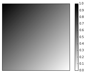
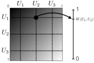
(a) left: Gradient graphon $W$; right: Schematic of sampling procedure

(b) $\mathbb{G}(50,W)$

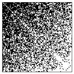
(c) $\mathbb{G}(100,W)$

(d) $\mathbb{G}(500,W)$

Figure 1: (a) An example of a graphon, given by the function $W(x,y)=\frac{(1-x)+(1-y)}{2}$. (b-d) top: Samples from the finite random graphs $\mathbb{G}(50,W)$, $\mathbb{G}(100,W),$ and $\mathbb{G}(500,W)$, shown as “pixel pictures” of the adjacency matrix, where black corresponds to $1$ and white to $0$; bottom: The samples resorted by increasing order of the sampled uniform random variables $U_{i}$.

1.1 Contributions

This paper presents two main contributions. We first show how digraphons can be used to model directed graphs, highlighting special cases that make use of dependence in the edge directions. In particular, we characterize the form of digraphons that produce tournaments, linear orderings, directed acyclic graphs, and partial orderings (Section 3). We briefly discuss how these formulations can be used to produce estimators for directed graph models (Section 3.3).

Next, we given an explicit example of a prior on digraphons: we present the infinite relational digraphon model (di-IRM), a Bayesian nonparametric block model for exchangeable directed graphs, which uses a Dirichlet process stick-breaking prior to partition the unit interval and Dirichlet-distributed weights for each pair of classes in the partition (Section 4). We derive a collapsed Gibbs sampling inference procedure (Section 6), and demonstrate applications of inference on synthetic data (Section 7), showing some limitations of using the infinite relational model with an asymmetric measurable function to model edge directions independently.

2 Background

We begin by defining notation and providing relevant background on directed exchangeable graphs. Our presentation largely follows Diaconis and Janson (2008).

2.1 Notation

Let $[n]:=\{1,\ldots,n\}$. For a directed graph (or digraph) $G$ whose vertex set $V$ is $[n]$ or ${{\mathbb{N}}}$, we write $(G_{ij})_{i,j\in V}$ for its adjacency matrix, i.e., $G_{ij}=1$ if there is an edge from vertex $i$ to vertex $j$, and 0 otherwise. We will omit mention of the set $V$ when it is clear. In general, for a directed graph, $(G_{ij})$ may be asymmetric, and we allow self-loops, which correspond to values $G_{ii}=1$ on the diagonal. The adjacency matrix of an undirected graph (without self-loops) is a symmetric array $(G_{ij})$ satisfying $G_{ii}=0$ for all $i$.

We write $X\stackrel{{\scriptstyle\mathrm{d}}}{{=}}Y$ to denote that the random variables $X$ and $Y$ are equal in distribution.

2.2 Exchangeability for directed graphs

A random (infinite) directed graph $G$ on ${{\mathbb{N}}}$ is exchangeable if its joint distribution is invariant under all permutations $\pi$ of the vertices:

$$(G_{ij})_{i,j\in\mathbb{N}}\stackrel{{\scriptstyle\mathrm{d}}}{{=}}(G_{\pi(i)\pi(j)})_{i,j\in\mathbb{N}}.$$ (2)

By the Kolmogorov extension theorem, it is equivalent to ask for this to hold only for those permutations $\pi$ that move a finite number of elements of ${{\mathbb{N}}}$.

Such an array $(G_{ij})$ is sometimes called jointly exchangeable. The case where the distribution is preserved under permutation of each index separately, i.e., where $(G_{ij})\stackrel{{\scriptstyle\mathrm{d}}}{{=}}(G_{\pi(i)\sigma(j)})$ for arbitrary permutations $\pi$ and $\sigma$, is called separately exchangeable, and arises for adjacency matrices of bipartite graphs.

2.3 Digraphons

As described by Diaconis and Janson (2008), using the Aldous–Hoover theorem one may show that every exchangeable countably infinite directed graph is expressible as a mixture of $\mathbb{G}({{\mathbb{N}}},\mathbf{W})$ with respect to some distribution on digraphons $\mathbf{W}$.

We now define digraphons; in Section 2.4 we will describe the sampling procedure that yields $\mathbb{G}({{\mathbb{N}}},\mathbf{W})$.

Definition 2.1.

A digraphon is a 5-tuple $\mathbf{W}:=(W_{00},W_{01},W_{10},W_{11},w)$, where $W_{ab}\colon[0,1]^{2}\rightarrow[0,1]$, for $a,b\in\{0,1\}$, and $w\colon[0,1]\rightarrow\{0,1\}$ are measurable functions satisfying the following conditions for all $x,y\in[0,1]$:

$$W_{00}(x,y) =W_{00}(y,x);$$

$$W_{11}(x,y) =W_{11}(y,x);$$ (3)

$$W_{01}(x,y) =W_{10}(y,x);$$

and

$$W_{00}(x,y)+W_{01}(x,y)+W_{10}(x,y)+W_{11}(x,y)=1.$$

Given a digraphon $\mathbf{W}$, write $\mathbf{W}_{4}$ for the map $[0,1]^{2}\rightarrow[0,1]^{4}$ given by $(W_{00},W_{01},W_{10},W_{11})$.

The functions $W_{ab}$ represent the joint probability of $G_{ij}=a$ and $G_{ji}=b$ for $a,b\in\{0,1\}$, i.e.,

$$\Pr(G_{ij}=a,G_{ji}=b)=W_{ab}(U_{i},U_{j}),$$ (4)

conditioned on $U_{i}$ and $U_{j}$. In this way, $W_{00}$ determines the probability of having neither edge direction between vertices $i$ and $j$, $W_{01}$ of only having a single edge to $j$ from $i$ (“right-to-left”), $W_{10}$ of a single edge from $i$ to $j$ (“left-to-right”), and $W_{11}$ of directed edges in both directions between $i$ to $j$. The function $w$ represents the probability of $G_{ii}$; because it is $\{0,1\}$-valued, this merely states whether or not $i$ has a self-loop.

(There is an equivalent alternative set of objects that may be used to specify an exchangeable digraph, where $W_{00},W_{01},W_{10},W_{11}$ are as before and $p\in[0,1]$ gives the marginal probability of a self-loop, which is independent of the other edges; see Diaconis and Janson (2008) for details.)

2.4 Sampling from a digraphon

The adjacency matrix $(G_{ij})_{i,j\in{{\mathbb{N}}}}$ of a countably infinite random graph $\mathbb{G}({{\mathbb{N}}},\mathbf{W})$ is determined by the following sampling procedure:

1. Draw $U_{i}\stackrel{{\scriptstyle\text{iid}}}{{\sim}}\text{Uniform}[0,1]$ for $i\in{{\mathbb{N}}}$.

2. For each pair of distinct vertices $i,j$, assign the edge values for $G_{ij}$ and $G_{ji}$ according to an independent $\text{Categorical}(\mathbf{W}_{4}(U_{i},U_{j}))$ such that Equation (4) holds.

3. Assign self-loops $G_{ii}=w(U_{i})$ for all $i$.

In other words, in step 2 we assign $(G_{ij},G_{ji})\,|\,U_{i},U_{j}\stackrel{{\scriptstyle\text{ind}}}{{\sim}}\text{Categorical}(\mathbf{W}_{4}(U_{i},U_{j}))$, where we interpret the categorical random variable as a distribution over the choices $(0,0),(0,1),(1,0),(1,1)$, in that order. Note that step 2 is well-defined by the symmetry condition in Equation (2.1). Figure 2 illustrates this sampling procedure via a schematic.

An analogous sampling procedure yields finite random digraphs: Given $n\in{{\mathbb{N}}}$, in step 1, instead sample only $U_{i}$ for $i\in[n]$. Then determine $G_{ij}$ for $i,j\in[n]$ as before. We write $\mathbb{G}(n,\mathbf{W})$ to denote the random digraph thereby induced on $[n]$.

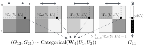
Figure 2: Schematic illustrating digraphon sampling procedure for $\mathbf{W}=(W_{00},W_{01},W_{10},W_{11},w)$. The $x$-axis is vertical and $y$-axis horizontal, with $(0,0)$ in the upper left, so that the notation $W_{ab}(x,y)$ coheres with the usual $(\text{row},\text{column})$ convention for matrix indexing.

2.5 Aldous–Hoover theorem for directed graphs

Diaconis and Janson (2008) derived the following corollary of the Aldous–Hoover theorem for directed graphs.

Theorem 2.2 (Diaconis–Janson).

Every exchangeable random countably infinite directed graph is obtained as a mixture of $\mathbb{G}({{\mathbb{N}}},\mathbf{W})$; in other words, as $\mathbb{G}({{\mathbb{N}}},\mathbf{W})$ for some random digraphon $\mathbf{W}$.

Therefore the problem of specifying the distribution of an infinite exchangeable digraph may be equivalently viewed as the problem of specifying a distribution on digraphons.

3 Digraphons and statistical modeling

We first motivate the use of digraphons instead of asymmetric measurable functions for modeling exchangeable directed graphs. We then discuss the representations via digraphons for several random structures which are special cases of directed graphs. Finally, we discuss how to estimate digraphons, in the context of both Bayesian and frequentist estimation.

3.1 Modeling limitations of asymmetric measurable functions

Asymmetric measurable functions $W_{\text{asym}}\colon[0,1]^{2}\rightarrow[0,1]$ characterize exchangeable bipartite graphs by the Aldous–Hoover theorem for separately exchangeable arrays; for details see Diaconis and Janson (2008, §8). These functions can also be used to generate and model directed graphs (without self-loops) by considering the edge directions $G_{ij}$ and $G_{ji}$ independently, i.e., $\Pr(G_{ij}=1)=W_{\text{asym}}(U_{i},U_{j})$ for all $i\neq j$, conditioned on $U_{i}$ and $U_{j}$, according to the following sampling procedure:

$$U_{i} \stackrel{{\scriptstyle\text{iid}}}{{\sim}}\text{Uniform}[0,1]\text{~{}for~{}}i\in{{\mathbb{N}}},$$

$$G_{ij}\,|\,U_{i},U_{j} \stackrel{{\scriptstyle\text{ind}}}{{\sim}}\text{Bernoulli}(W_{\text{asym}}(U_{i},U_{j})),\text{~{}for $i\neq j$},$$

and $G_{ii}=0$ for $i\in{{\mathbb{N}}}$. Currently priors on these asymmetric functions are popular in Bayesian modeling of directed graphs, as we note in Section 5.

Asymmetric measurable functions are also equivalent to the following special case of the digraphon representation. Via the above sampling procedure, every asymmetric measurable function $W_{\text{asym}}$ yields the same directed graph as the digraphon $\mathbf{W}=(W_{00},W_{01},W_{10},W_{11},w)$ given pointwise by

$$\mathbf{W}(x,y)=((1-p)(1-q),\,(1-p)q,\,p(1-q),\,pq,\,0),$$

where $p:=W_{\text{asym}}(x,y)$ and $q:=W_{\text{asym}}(y,x)$. In particular, conditioned on $x=U_{i}$ and $y=U_{j}$, the marginal probability $p(1-q)+pq=p$ of an edge from $i$ to $j$ and $(1-p)q+pq=q$ of an edge from $j$ to $i$ are independent.

On the other hand, many common kinds of digraphs are not obtainable from a single asymmetric function. Consider the following two classes:

1. Undirected graphs: between any two vertices $i$ and $j$, there are either no edges ($G_{ij}=G_{ji}=0$), or edges in both directions ($G_{ij}=G_{ji}=1$).

2. Tournaments: between any two vertices $i$ and $j$, there is exactly one directed edge, i.e., $G_{ij}=1$ or $G_{ji}=1$ but not both.

For digraphs of either of these two sorts, the directions are correlated, and hence not obtainable from the above sampling procedure for an asymmetric measurable function, as this procedure generates $G_{ij}$ and $G_{ji}$ independently. This demonstrates how the use of an asymmetric measurable function is poorly suited for graphs with correlated edge directions. Though constructing a model for general digraphs using the function $W_{\text{asym}}$ leads to misspecification, one might hope to perform inference nevertheless; however, as we show in Section 7.2, doing so may fail to discern structure that may be discovered through posterior inference with respect to a prior on digraphons.

In contrast to the use of asymmetric measurable functions, where one considers edge directions independently, with digraphons one considers the edge directions between vertex $i$ and vertex $j$ jointly, as in Equation (4). Thus, digraphons give a more general and flexible representation for modeling digraphs.

3.2 Special cases

We discuss several special cases of directed graphs and specify the form of their digraphon representations.

3.2.1 Undirected graphs

Undirected graphs can be viewed as directed graphs with no self-loops, where each pair of distinct vertices either has edges in both directions or in neither. Hence a digraphon that yields an undirected graph is one having no probability in the single edge directions, i.e., such that $W_{01}=W_{10}=0$ (or equivalently, $W_{00}+W_{11}=1$) and $w=0$. Such a digraph is therefore determined by merely specifying the graphon $W_{11}$, where $W_{00}=1-W_{11}$ is implicit.

Example 3.1.

In Figure 3, we display an example of a digraphon whose samples are undirected Erdős–Rényi graphs with edge density $\nicefrac{{1}}{{2}}$, i.e.,

$$(W_{00},W_{01},W_{10},W_{11},w)=\left(\nicefrac{{1}}{{2}},0,0,\nicefrac{{1}}{{2}},0\right).$$

This digraphon corresponds to the graphon $W(x,y)=\nicefrac{{1}}{{2}}$.

Figure 3: left: Erdős–Rényi undirected graph as a digraphon $\mathbf{W}$; right: $\mathbb{G}(20,\mathbf{W})$

3.2.2 Tournaments

A tournament is a directed graph without self-loops, where for each pair of vertices, there is an edge in exactly one direction. In other words, a tournament has $G_{ij}=1$ if and only if $G_{ji}=0$ for $i\neq j$, and $G_{ii}=0$. Therefore a digraphon yielding a tournament is one satisfying $w=0$ and $W_{01}+W_{10}=1$ (or equivalently, $W_{00}=W_{11}=0$).

Example 3.2.

An example of a tournament digraphon is displayed in Figure 4:

$$(W_{00},W_{01},W_{10},W_{11},w)=\left(0,\nicefrac{{1}}{{2}},\nicefrac{{1}}{{2}},0,0\right).$$

The random tournament induced by sampling from this digraphon is almost surely isomorphic to a countable structure known as the generic tournament. (For more details on this example, see Chung and Graham (1991) and Diaconis and Janson (2008, Example 9.2).)

As discussed in Section 3.2.1, exchangeable undirected graphs can be specified in terms of single functions $W_{11}$ (graphons) and their associated sampling procedure (described in Equation 1). Similarly, tournaments also have a single-function representation and associated sampling procedure. Namely, a tournament digraphon is determined by a measurable function $W_{T}:[0,1]^{2}\rightarrow[0,1]$ that is anti-symmetric in the sense that $W_{T}(x,y)=1-W_{T}(y,x)$ for all $x,y\in[0,1]$ (corresponding to the digraphon condition $W_{01}(x,y)=W_{10}(y,x)$). To sample from $W_{T}$, first sample $G_{ij}\,|\,U_{i},U_{j}\stackrel{{\scriptstyle\text{ind}}}{{\sim}}\text{Bernoulli}(W_{T}(U_{i},U_{j}))$ for $i<j$, and then set $G_{ji}=1-G_{ij}$ (and $G_{ii}=0$). The digraphon in Example 3.2 corresponds to the anti-symmetric, measurable function $W_{T}(x,y)=\nicefrac{{1}}{{2}}$.

Tournament digraphons have recently been studied in detail by Thörnblad (2016), which calls the single function $W_{T}$ a tournament kernel.

Statistical models for tournaments appear in the ranking theory literature, often using a variant of the Bradley–Terry model (Bradley and Terry, 1952), first described by Zermelo (1929). For more details, including the relation to graphons, see Chatterjee (2015, §2.7). This literature, and related estimation papers such as Chatterjee and Mukherjee (2016), is also often framed in terms of a single-function representation.

Figure 4: left: Digraphon $\mathbf{W}$ that yields a generic tournament; right: $\mathbb{G}(20,\mathbf{W})$

3.2.3 Linearly ordered sets

A digraph is a (strict) linear ordering when the directed edge relation is transitive, and every pair of distinct vertices has an edge in exactly one direction. Consider the digraphon given by $W_{00}=W_{11}=w=0$ and $W_{01}=1-W_{10}$, where

$$W_{10}(x,y)=\begin{cases}1&\text{~{}if~{}}x<y,\\ 0&\text{~{}otherwise}.\end{cases}$$

The countable directed graph induced by sampling from this digraphon is almost surely a linear order. In fact, this is essentially the only such example — by Glasner and Weiss (2002, §8), its distribution is the same as that of every exchangeable linear ordering. (In other words, any digraphon yielding the (unique) exchangeable linear ordering is weakly isomorphic to this one; see Section 7 for details.) Furthermore, the countable linear ordering obtained from sampling this digraphon is almost surely dense and without endpoints, and hence isomorphic to the rationals. A finite sample with $n$ vertices has distribution equal to the uniform measure on all $n!$ ways of linearly ordering $\{1,\ldots,n\}$.

This digraphon is displayed in Figure 5 alongside a 20 vertex random sample, rearranged by increasing $U_{i}$; note that for almost every sample, the corresponding rearranged graph will have all vertices strictly above the diagonal.

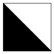
Figure 5: left: Linear ordering digraphon; right: $\mathbb{G}(20,\mathbf{W})$

3.2.4 Directed acyclic graphs

A directed acyclic graph (DAG) is a directed graph having no directed path from any vertex to itself. Various work has focused on models for DAGs (e.g., see Roverato and Consonni (2004)), and especially their use in describing random instances of directed graphical models (also known as Bayesian networks). DAGs also arise naturally as networks describing non-circular dependencies (e.g., among software packages), and in other key data structures.

One can show, using the main result of Hladký et al. (2015) (which we describe in Section 3.2.5), that any exchangeable DAG can be obtained from sampling a digraphon satisfying $W_{10}(x,y)=0$ for $x\geq y$ and $W_{11}=w=0$. Note that this constrains the digraphon to have the same zero-valued regions as those in the canonical presentation of a linear ordering digraphon (as described above and displayed in Figure 5), except that $W_{00}$ may be arbitrary. (Equivalently, for $x<y$, the value $W_{10}(x,y)$ may be chosen arbitrarily, so that the remaining terms are given by $W_{01}(x,y)=W_{10}(y,x)$ and $W_{00}=1-W_{01}-W_{10}$.) A digraphon of this form thereby specifies one way in which the exchangeable DAG can be topologically ordered (i.e., extended to some exchangeable linear ordering).

Specifying a digraphon in this way always yields a DAG upon sampling, as the standard linear ordering on $[0,1]$ does not admit directed cycles, and one can show that all exchangeable DAGs arise in this way, as mentioned above.

Example 3.3.

An example of a digraphon that yields exchangeable DAGs is the generic DAG digraphon given by

$$W_{00} =\nicefrac{{1}}{{2}},$$

$$W_{10}(x,y) =\begin{cases}\nicefrac{{1}}{{2}}&\text{~{}if~{}}x<y,\\ 0&\text{~{}otherwise, and}\end{cases}$$

$$W_{11} =0,$$

where $W_{01}$ is such that $W_{01}(x,y)=W_{10}(y,x)$. This example is displayed in Figure 6. We can see that the reordered sample is indeed a DAG, as the edges clearly all lie above the diagonal in the adjacency matrix.

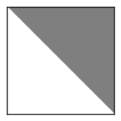
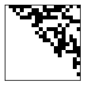
Figure 6: left: Example of a DAG digraphon; right: $\mathbb{G}(20,\mathbf{W})$

3.2.5 Partially ordered sets

A partially ordered set, or poset, is a set with a binary relation $\preceq$ that is reflexive, antisymmetric, and transitive. A poset can be viewed as a digraph having a directed edge from $a$ to $b$ if and only if $a\preceq b$. Note that the transitive closure of any DAG is a poset, i.e., if in a DAG, there is a directed path from $a$ to $b$, the transitive closure has an edge from $a$ to $b$, thereby producing a partial ordering. (One can similarly define the “transitive closure digraphon” of a digraphon that yields DAGs to obtain a digraphon yielding the corresponding transitive closures). Conversely, any poset (with self-loops removed) is already a DAG. Therefore exchangeable posets are obtainable by some digraphon of the form described in Section 3.2.4 (except with $w=1$), though not all such digraphons yield posets. Analogously, representing an exchangeable poset via a digraphon of this form amounts to specifying a linearization of the poset.

Janson (2011) develops a theory of poset limits (or posetons) and their relation to exchangeable posets. By Hladký et al. (2015), any exchangeable poset is given by some digraphon $\mathbf{W}$ for which $W_{10}(x,y)>0$ implies that $x<y$, i.e., $\mathbf{W}$ is compatible with the standard linear ordering on $[0,1]$.

Example 3.4.

Consider the following example of a digraphon that yields an exchangeable poset, specified by the following blockmodel:

$$W_{10} =\begin{cases}\nicefrac{{1}}{{2}}&\text{~{}if~{}}x<\nicefrac{{1}}{{4}}\text{~{}and~{}}\nicefrac{{1}}{{4}}\leq y<\nicefrac{{3}}{{4}},\\ \nicefrac{{1}}{{2}}&\text{~{}if~{}}\nicefrac{{1}}{{4}}\leq x<\nicefrac{{3}}{{4}}\text{~{}and~{}}y\geq\nicefrac{{3}}{{4}},\\ 1&\text{~{}if~{}}x<\nicefrac{{1}}{{4}}\text{~{}and~{}}y\geq\nicefrac{{3}}{{4}}\text{, and}\\ 0&\text{~{}otherwise,}\end{cases}$$

where $W_{11}=0$, where $W_{01}$ is such that $W_{01}(x,y)=W_{10}(y,x)$, and where $W_{00}=1-W_{01}-W_{10}$.

This example is displayed in Figure 7. In particular, the block structure of the model is reflected in the rearranged sample on the right. We can see that this is an exchangeable poset: if the loops (the diagonal) are removed from this digraph, it is a DAG (as all the edges in the rearranged sample are above the diagonal), and one can check that it is transitively closed.

This is a key example among posets. Work of Kleitman and Rothschild (1975) and Compton (1988), characterizing the combinatorial structure of a typical large finite poset, implies that the sequence of uniform distributions on labeled posets of size $n$ converges (in the sense of poset limits) to this example.

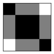
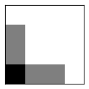
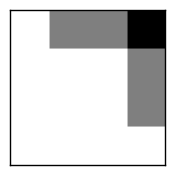
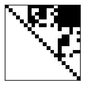
Figure 7: left: Example of a $3\times 3$ SBM poset digraphon; right: $\mathbb{G}(20,\mathbf{W})$

3.3 Digraphon estimation

For undirected graphs, the graphon estimation problem has received considerable attention in recent years. In graphon estimation, one seeks to infer either the function $W$, or the associated probability matrix with entries $M_{ij}:=W(U_{i},U_{j})$, given a single sample (or multiple samples) of the graph. From the Bayesian modeling perspective, one places a prior on graphons and performs an inference procedure to estimate the parameters of the random function prior.

From the frequentist perspective, one is interested in producing an estimator for a fixed graphon, and many such algorithms have been developed, including histogram and degree-sorting based methods. To produce a frequentist digraphon estimator, one can extend methods developed for graphons. Just as a single asymmetric measurable function is insufficient for representing correlated edge directions, one must likewise estimate the edge directions jointly. Although a directed graph can be simply represented with a single asymmetric matrix, digraphon estimators must consider the impact on pairs of entries $(G_{ij},G_{ji})$ jointly when partitioning, rearranging, or otherwise manipulating vertices $i,j$.

Histogram estimators for digraphons

A histogram estimation procedure for graphons partitions the vertices into several classes, and then uses the average edge density across each pair of classes as an estimate of the probability of an edge between two vertices in those classes. This reduces the problem to that of estimating a partition that yields a good estimate of these edge densities. Many methods have been developed for this problem; for further details see the references within Borgs et al. (2015, §§1.3 and 1.7).

To estimate a digraphon (ignoring loops), we must estimate four edge-direction histograms, where the goal is to estimate a partition of the vertices that simultaneously yields good estimates of the four types of edge densities. After producing a partition of the vertices, one likewise computes the average edge density in each of the four cases, resulting in four histograms. (If considering loops, there is one additional 1-dimensional histogram whose estimates are to be jointly optimized by the partition.)

The Frieze–Kannan and Szemerédi regularity lemmas lead to bounds on how well a large graph can be approximated using edge densities across a partition (Lovász, 2012, Chapters 9 and 10); see also Kallenberg (1999). The generalization of the Szemerédi regularity lemma to directed graphs by Alon and Shapira (2004) likewise provides a bound in terms of directed edge densities.

Degree-sorting estimators for digraphons

Many degree-sorting algorithms have been proposed for graphon estimation. These algorithms often involve “sorting” followed by “smoothing”. In the sorting step, the vertices are sorted by their degrees, where the degree of a vertex $i$ is defined to be $\sum_{j=1}^{n}G_{ij}$, In the smoothing step, the $\{0,1\}$-valued adjacency matrix is used to produce a $[0,1]$-valued matrix using some smoothing algorithm. For example, Chan and Airoldi (2014) compare a degree-sorting algorithm that uses total variation distance minimization as a smoothing step to one that uses universal singular value thresholding (Chatterjee, 2015) as the smoothing step. Degree-sorting estimators assume that the degree distribution $\int_{0}^{1}W(x,y)dy$ is strictly monotonizable in $x$, i.e., in order for sorting to be effective, the degrees of the vertices must vary.

This idea can be similarly applied to digraphon estimation: First sort the degrees of the vertices by the four types of edge directions, to obtain four adjacency matrices, and then smooth these matrices. It would suffice to require, after possibly applying a single measure-preserving transformation to $[0,1]$, that the map $x\mapsto\bigl{(}\int_{0}^{1}W_{00}(x,y)dy,\int_{0}^{1}W_{01}(x,y)dy,\int_{0}^{1}W_{10}(x,y)dy,\int_{0}^{1}W_{11}(x,y)dy\bigr{)}$ is strictly increasing with respect to the lexicographic ordering of $[0,1]^{4}$.

In this paper, we do not comment further on digraphon estimators, but many other graphon estimation techniques should generalize similarly. One way of describing the general pattern is to jointly consider the corresponding techniques applied to the four matrices obtained from the adjacency matrix restricted to each joint edge type.

Priors on digraphons

Bayesian approaches may also be use to estimate a digraphon; this is the focus of much of the rest of the paper. One may likewise use similar techniques to those that have been developed for graphons. Analogously to the case of undirected graphs, a Bayesian model for exchangeable directed graphs involves placing a prior on digraphons. This is justified by the characterization in Section 2.5 of exchangeable directed graphs in terms of random digraphons. We discuss such an approach in depth in Section 4, where we present a Bayesian nonparametric model based on random partitions using the Dirichlet process.

4 Infinite relational digraphon model

We now proceed to describe a prior on digraphons that makes use of block structure. For directed graphs, the infinite relational model (IRM) (Kemp et al., 2006) models edges between vertices using an asymmetric measurable function and is a nonparametric extension of the (asymmetric) stochastic block model. In this section, we present the infinite relational digraphon model (di-IRM), which gives a prior on digraphons. This model can be viewed as a generalization of the symmetric IRM, a graphon model, to the digraphon case. We then show how the di-IRM can be used to model a variety of digraphs, including ones that cannot be modeled using an asymmetric IRM.

4.1 Generative model

We present two equivalent representations of the di-IRM model: (1) a digraphon representation and (2) a clustering representation. The digraphon representation uses a stick-breaking Dirichlet process prior to partition the unit interval, while the clustering representation uses a Chinese restaurant process prior to partition the vertices. The difference between the two representations is analogous to that between the representations of the IRM given by Orbanz and Roy (2015, §4.1).

4.1.1 Digraphon representation

We first introduce some notation. Let $\alpha>0$ be a concentration hyperparameter, and $\boldsymbol{\beta}:=(\beta^{(00)},\beta^{(01)},\beta^{(10)},\beta^{(11)})$ be a hyperparameter vector for the weight matrices $\boldsymbol{\eta}:=(\boldsymbol{\eta}^{(00)},\boldsymbol{\eta}^{(01)},\boldsymbol{\eta}^{(10)},\boldsymbol{\eta}^{(11)})$, where $\beta^{(ab)}\in[0,\infty)$ for $a,b\in\{0,1\}$. We allow some (but not all) of the Dirichlet parameters to take the value zero, at which the corresponding components must be degenerate. As a shorthand, we write $\boldsymbol{\eta}_{r,s}:=(\eta^{(00)}_{r,s},\eta^{(01)}_{r,s},\eta^{(10)}_{r,s},\eta^{(11)}_{r,s})$ for the 4-tuple of weights of the classes $r$ and $s$, where $r,s\in{{\mathbb{N}}}$. The following generative process gives a prior on digraphons:

1. Draw a partition of $[0,1]$:

   $$\boldsymbol{\Pi}\,|\,\alpha\sim\text{DP-Stick}(\alpha).$$

2. Draw weights for each pair of classes $(r,s)$ of the partition:

   1. Draw weights for the upper diagonal blocks, where $r<s$:

      $$\boldsymbol{\eta}_{r,s}\,|\,\boldsymbol{\beta}\sim\text{Dirichlet}(\boldsymbol{\beta}).$$

   2. Draw weights for the diagonal blocks:

      $$(\eta_{r,r}^{(00)},\eta_{r,r}^{(01)}+\eta_{r,r}^{(10)},\eta_{r,r}^{(11)})\ |\ \boldsymbol{\beta} \sim\text{Dirichlet}(\beta^{(00)},\,\beta^{(01)}+\beta^{(10)},\,\beta^{(11)}),$$

      subject to the constraint

      $$\eta_{r,r}^{(01)} =\eta_{r,r}^{(10)}.$$

   3. Set weights for the lower diagonal blocks, where $r>s$, such that the symmetry requirements in Equation (2.1) are satisfied:

      $$\eta^{(00)}_{r,s} =\eta^{(00)}_{s,r},\quad\eta^{(11)}_{r,s}=\eta^{(11)}_{s,r},$$

      $$\eta^{(01)}_{r,s} =\eta^{(10)}_{s,r},\quad\eta^{(10)}_{r,s}=\eta^{(01)}_{s,r}.$$

In Section 4.2 we show different types of random digraphons that arise from various settings of $\boldsymbol{\beta}$. The partition is drawn from a Dirichlet stick-breaking process: for each $i\in{{\mathbb{N}}}$, draw $X_{i}\stackrel{{\scriptstyle\text{iid}}}{{\sim}}\text{Beta}(1,\alpha)$, and for every $k\in{{\mathbb{N}}}$, set $V_{k}=X_{k}\prod_{i=1}^{k-1}(1-X_{i})$, so that $\sum_{k=1}^{\infty}V_{k}=1$, thereby determining a random partition of $[0,1]$.

The self-loops can be specified using the same partition of $[0,1]$, either with a deterministic $\{0,1\}$-valued function $w$ or a single weight $p$, as described in Section 2.3. For our purposes, we assume $w=0$. This generative process fully specifies a random digraphon $\mathbf{W}$, from which random digraphs $\mathbb{G}(n,\mathbf{W})$ can then be sampled according to the process given in Section 2.4.

4.1.2 Clustering representation

An alternative representation of the generative process for a partition described above can be formulated directly in terms of clustering: in this generative process, each vertex $i$ has a cluster assignment $z_{i}$. This yields an equivalent assignment to that given by the digraphon formulation if, after sampling the uniform random variable $U_{i}$, we assign vertex $i$ to the cluster corresponding to the class of the partition of $[0,1]$ that $U_{i}$ belongs to.

Thus, in place of the first step of the generative process given in the digraphon representation (Section 4.1.1), we draw a partition of the vertices from a Chinese restaurant process (CRP) (as described in, e.g., Aldous (1985)): $\mathbf{z}\sim\text{CRP($\alpha$)},$ where each $z_{i}$ gives the cluster assignment of vertex $i$, and $\alpha>0$ is a hyperparameter. The weights $\boldsymbol{\eta}$ are drawn in the same manner as in the second step of the digraphon representation of the di-IRM. Finally, edges are drawn analogously to the general digraphon sampling procedure: $(G_{ij},G_{ji})\stackrel{{\scriptstyle\text{ind}}}{{\sim}}\text{Categorical}(\boldsymbol{\eta}_{z_{i},z_{j}})$, so that Equation (4) holds, where again the Categorical distribution is over the choices $(0,0),(0,1),(1,0),(1,1)$.

This representation is particularly convenient for performing inference, especially when using a collapsed Gibbs sampling procedure, as we show in Section 6.

4.2 Special cases obtained from the di-IRM

In Figure 8, we display examples of random di-IRM draws using several settings of the hyperparameter vector $\boldsymbol{\beta}$. The parameter settings were specifically chosen to illustrate some of the special cases the di-IRM model can cover.

(a) Undirected: $\beta^{(01)}=\beta^{(10)}=0$

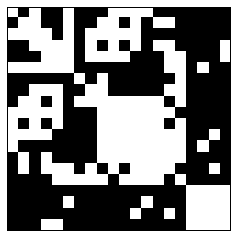
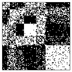
(b) $\mathbb{G}(20,\mathbf{W})$, $\mathbb{G}(100,\mathbf{W})$

(c) Tournament: $\boldsymbol{\beta}=(0,2,1,0)$

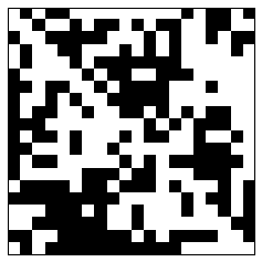
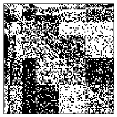
(d) $\mathbb{G}(20,\mathbf{W})$, $\mathbb{G}(100,\mathbf{W})$

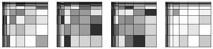
(e) Correlated directions: $\boldsymbol{\beta}=(0.9,2,1,0.5)$

(f) $\mathbb{G}(20,\mathbf{W})$, $\mathbb{G}(100,\mathbf{W})$

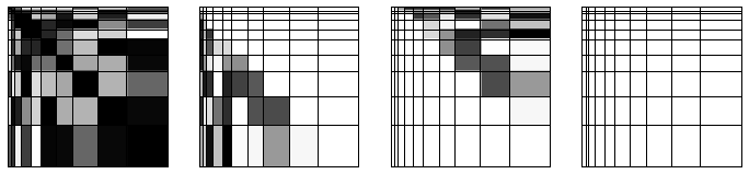
(g) Acyclic: $\boldsymbol{\beta}=(0.5,0,0.5,0)$

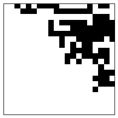
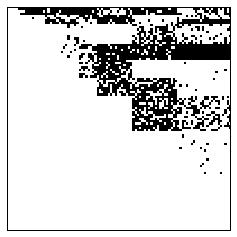
(h) $\mathbb{G}(20,\mathbf{W})$, $\mathbb{G}(100,\mathbf{W})$

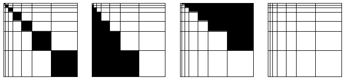
(i) Near-ordering: $\boldsymbol{\beta}=(0,0,1,0)$

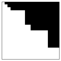
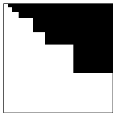
(j) $\mathbb{G}(20,\mathbf{W})$, $\mathbb{G}(100,\mathbf{W})$

Figure 8: Each row shows a random digraphon drawn from the di-IRM prior along with a 20-vertex sample and a 100-vertex sample, arranged in order of increasing $U_{i}$. In the smaller samples, one can see certain properties of the digraph (e.g., that (b) is symmetric and (d) is a tournament), while in the larger samples one can discern block structure with approximate edge densities. For (g) and (i), the values given for $\boldsymbol{\beta}$ only apply to the classes $r\neq s$, and instead the tuple of hyperparmeters $\boldsymbol{\beta}_{r}=(1,0,0)$ is used for the diagonal.

Undirected

To get a prior on graphons using the di-IRM, we can set $\beta^{(01)}=\beta^{(10)}=0$. Figure 8(a) shows a parameter setting that produces undirected graphs and is equivalent to a symmetric IRM when taking $W_{11}$ to be the IRM; we can see from the sample on the right that the graph is indeed undirected.

Tournaments

We can specify a di-IRM tournament prior by setting $\beta^{(00)}=\beta^{(11)}=0$. Figure 8(c) shows the parameter setting $\boldsymbol{\beta}=(0,2,1,0)$, which puts all the mass on the middle two functions. The tournament structure is easy to see in the 20-vertex sample; for distinct $i$ and $j$, whenever there is an edge from $i$ to $j$, there is not an edge from $j$ to $i$.

Figure 8(e) shows a less extreme (non-tournament) variant that still has strong correlations between the edge directions, by virtue of retaining most of the mass on the functions $W_{01}$ and $W_{10}$. Here we set $\boldsymbol{\beta}=(0.9,2,1,0.5)$. Note that the block structure in a sample from this digraphon is more subtle than in the undirected sample, demonstrating the importance of counting all four edge-direction combinations rather than just marginals for the two directions.

Directed acyclic graphs

To obtain a directed acyclic graph from the di-IRM, we set the hyperparameters so that the resulting function $W_{11}$ is empty and $W_{10}$ has nonzero values only on blocks above the diagonal, as in Section 3.2.4. To achieve this, we set the Dirichlet weight parameters $\boldsymbol{\beta}$ such that $\beta^{(01)}=\beta^{(11)}=0$ for the weights $\boldsymbol{\eta}_{r,s}$ where $r\neq s$, and for each class $r$ let $\boldsymbol{\beta}_{r}$ refer to the 3-tuple of hyperparameters used for the $\boldsymbol{\eta}_{r,r}$ weights on the diagonal, each set to $\boldsymbol{\beta}_{r}=(1,0,0)$. With these hyperparameter choices, we obtain a directed acyclic di-IRM, as seen in Figure 8(g). We can see in both samples that the directed edges in the resorted sample lie above the diagonal. Note that we make use of $\boldsymbol{\beta}_{r}$ only in this section, to show how to get a DAG prior; in our later inference examples, we use the di-IRM model as introduced in the previous subsection with the single vector of hyperparameters $\boldsymbol{\beta}$.

Near-ordering

Consider the hyperparameter settings $\boldsymbol{\beta}=(0,0,1,0)$ for the weights $\boldsymbol{\eta}_{r,s}$ when $r\neq s$, and $\boldsymbol{\beta}_{r}=(1,0,0)$ for every class $r$. The resulting digraph is “nearly” ordered, in the sense that it is linearizable and any two elements in different classes are comparable, as seen in Figure 8(i). Here $\eta^{(10)}_{r,s}=1$ for any blocks $(r,s)$ above the diagonal, and the resulting partial ordering is apparent in both of the resorted samples, with all directed edges above the diagonal.

4.3 Other partitions for the di-IRM

Any block model digraphon can be specified in a similar manner: first define a partition of $[0,1]$, which then gives a partition of $[0,1]^{2}$; next let each block on $[0,1]^{2}$ be piecewise constant such that the symmetry requirements in Equation (2.1) are satisfied.

In the case where the number of classes and the size of the classes are fixed parameters, the directed IRM behaves similarly to some random directed SBM. In addition to the CRP, we can also consider other partitioning schemes. Alternatively, one can consider other random partitions of $[0,1]$ as well. For instance, if one is interested in power law scaling in the number of clusters (and the sizes of particular clusters), the Pitman–Yor process (Pitman and Yor, 1997) provides a suitable generalization of the Dirichlet process. It has both a stick-breaking and urn representation analogous to those for the Dirichlet process.

5 Related work

The stochastic block model (see Holland et al. (1983) and Wasserman and Faust (1994)) has been well-studied in the case of directed graphs (Holland and Leinhardt, 1981; Wang and Wong, 1987), including from a Bayesian perspective (Wong, 1987; Gill and Swartz, 2004; Nowicki and Snijders, 2001). Although working within a restricted class of models, already Holland and Leinhardt (1981) consider the full joint distribution on edge directions, rather than making independence assumptions.

The directed stochastic blockmodel (di-SBM) can be represented as a digraphon $\mathbf{W}_{4}$ given by four step-functions that are piecewise constant on a finite number of classes. We display an example of a directed SBM in Figure 9. The di-IRM model presented in this paper can be seen as a nonparametric extension of the di-SBM, just as the undirected IRM (introduced independently by Kemp et al. (2006) and Xu et al. (2007)) is a nonparametric undirected SBM.

Any prior on exchangeable undirected graphs can be described in terms of a corresponding prior on graphons. As alluded to in the introduction, many Bayesian nonparametric models for graphs admit a nice representation in this form (even if not originally described in these terms); see Orbanz and Roy (2015, §4) for additional details and examples from the machine learning literature, including the IRM. Likewise, priors on exchangeable digraphs (which have been less thoroughly explored) can be described in terms of the corresponding priors of digraphons, as we have begun to do here.

As noted in Lloyd et al. (2012), when existing models are expressed in these terms, various restrictions (and in particular, unnecessary independence assumptions) become more apparent. As we have seen, the use of the IRM on directed graphs models the edge directions as independent (see Kemp et al. (2004) for examples), a condition that can be straightforwardly relaxed when the model is expressed in the general setting provided by digraphons.

Exchangeable directed graphs have also been considered by Austin (2008), via an application of the Aldous–Hoover theorem, although this work does not describe digraphons explicitly. We conclude this section by describing several extensions of the graphon formalism, some of which can be combined with the directed case. In particular, edges may be more general than $\{0,1\}$-valued. Variants of graphons for weighted and edge-colored graphs have been considered by Lovász (2012, Chapter 17) and Austin (2008). Graphs with edge multiplicity, or multigraphs, can be viewed as integer-valued arrays, a case also covered by the Aldous–Hoover theorem, although the corresponding extension of graphons is more complicated when the edge multiplicities are unbounded; see Kolossváry and Ráth (2011), Lovász (2012, Chapter 17), and Kunszenti-Kovács et al. (2014). Graphs (that are not necessarily symmetric) with real-valued edges are also covered by the Aldous–Hoover theorem through real-valued exchangeable arrays, and have many applications in statistics and machine learning; see Lloyd et al. (2012) and Orbanz and Roy (2015). The Aldous–Hoover theorem also covers real-valued $d$-dimensional arrays for $d>2$, although the corresponding extension of graphons to the case of hypergraphs is considerably more involved; for details, see Lovász (2012, Chapter 23.3), Austin (2008), and Lloyd et al. (2013).

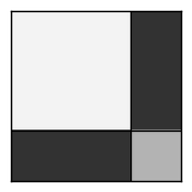
(a) $W_{00}$

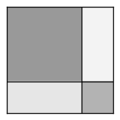
(b) $W_{01}$

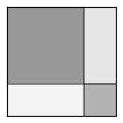
(c) $W_{10}$

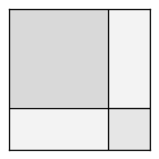
(d) $W_{11}$

(e) $w$

Figure 9: Example of a directed stochastic block model digraphon with 2 classes and a 0.7 division. This example is assortative, i.e., there are more edges within the same group than between different groups.

6 Posterior inference

In this section, we perform collapsed Gibbs sampling for the di-IRM. We use the notation for the clustering representation of the di-IRM, so we can use Gibbs sampling to repeatedly sample the cluster assignment of each vertex.

Let $G$ be a digraph on $[n]$; for simplicity we assume that $G$ has no self-edges, and that, as in Section 4.1.1, the di-IRM parameters are chosen so that no self-edges are produced. Consider a partition of $[n]$ into a countably infinite number of clusters, and for $i\in[n]$, let $z_{i}\in{{\mathbb{N}}}$ denote the cluster assignment of $i$. Write $\mathbf{z}$ for the vector of all cluster assignments, and $\boldsymbol{\eta}$ for the 4-tuple of weight matrices. Because of the symmetry requirement of the diagonal, we are able to simplify notation as follows: let $m_{r}^{*}:=m_{r,r}^{(01)}+m_{r,r}^{(10)}$, let $\eta_{r}^{*}:=\eta_{r,r}^{(01)}+\eta_{r,r}^{(10)}$, and let $\beta^{*}:=\beta^{(01)}+\beta^{(10)}$. Let $\boldsymbol{\beta}^{*}:=(\beta^{(00)},\beta^{*},\beta^{(11)})$ be the 3-tuple of hyperparameters for the diagonal blocks.

The likelihood of $G$ being drawn from the di-IRM, given cluster assignments $\mathbf{z}$ and weights $\boldsymbol{\eta}$, is given by

$$p(G\,|\,\mathbf{z},\boldsymbol{\eta}) =\prod_{r\leq s}\prod_{a,b}(\eta_{r,s}^{(ab)})^{m_{r,s}^{(ab)}}$$

$$=\Bigl{[}\prod_{r<s}\prod_{a,b}(\eta_{r,s}^{(ab)})^{m_{r,s}^{(ab)}}\Bigr{]}\,\Bigl{[}\prod_{r}(\eta_{r,r}^{(00)})^{m_{r,r}^{(00)}}(\textstyle\frac{1}{2}\eta_{r}^{*})^{m_{r}^{*}}(\eta_{r,r}^{(11)})^{m_{r,r}^{(11)}}\Bigr{]},$$

where $m_{r,s}^{(ab)}$ denotes the number of directed edges of type $(ab)$ between class $r$ and class $s$, for $a,b\in\{0,1\}$ and $r,s\in{{\mathbb{N}}}$.

Since the weights $\boldsymbol{\eta}$ have a factorized Dirichlet distribution prior, we have

$$p(\boldsymbol{\eta}\,|\,\boldsymbol{\beta}) =\Bigl{[}\textbf{B}(\boldsymbol{\beta})^{-1}\prod_{r<s}\prod_{a,b}(\eta_{r,s}^{(ab)})^{\beta^{(ab)}-1}\Bigr{]}$$

$$\quad\times\Bigl{[}\textbf{B}(\boldsymbol{\beta}^{*})^{-1}\prod_{r}(\eta_{r,r}^{(00)})^{\beta^{(00)}-1}(\eta_{r}^{*})^{\beta^{*}-1}(\eta_{r,r}^{(11)})^{\beta^{(11)}-1}\Bigr{]},$$

where $\textbf{B}(\boldsymbol{\theta}):=\frac{\prod_{i}\Gamma(\theta_{i})}{\Gamma(\sum_{i}\theta_{i})}$ is the multivariate beta function.

We sample each cluster assignment $z_{i}$ conditional on all other assignment variables:

$$z_{i}\,|\,\mathbf{z}_{-i}\sim p(z_{i}\,|\,\mathbf{z}_{-i},G)\propto p(G|\mathbf{z})\,p(z_{i}|\mathbf{z}_{-i}),$$ (5)

where $\mathbf{z}_{-i}$ denotes the vector of all assignments $z_{j}$ such that $j\neq i$.

To compute the first term in Equation (5), we can integrate out the parameters $\eta_{r,s}^{(ab)}$:

$$p(G\,|\,\mathbf{z}) =\Bigl{[}\textbf{B}(\boldsymbol{\beta})^{-1}\prod_{r<s}\int\prod_{a,b}(\eta_{r,s}^{(ab)})^{m_{r,s}^{(ab)}+\beta^{(ab)}-1}\,d\eta_{r,s}^{(ab)}\Bigr{]}$$

$$\quad\,\,\times\biggl{[}\textbf{B}(\boldsymbol{\beta}^{*})^{-1}\prod_{r}2^{-m_{r}^{*}}\,$$

$$\qquad\qquad\qquad\int(\eta_{r,r}^{(00)})^{m_{r,r}^{(00)}+\beta^{(00)}-1}(\eta_{r}^{*})^{m_{r}^{*}+\beta^{*}-1}(\eta_{r,r}^{(11)})^{m_{r,r}^{(11)}+\beta^{(11)}-1}\,d\boldsymbol{\eta}_{r}\biggr{]}$$

$$=\Bigl{[}\textbf{B}(\boldsymbol{\beta})^{-1}\,\prod_{r<s}\textbf{B}(\textbf{m}_{r,s}+\boldsymbol{\beta})\Bigr{]}\Bigl{[}\textbf{B}(\boldsymbol{\beta}^{*})^{-1}\,\prod_{r}2^{-m_{r}^{*}}\,\textbf{B}(\textbf{m}_{r}+\boldsymbol{\beta}^{*})\Bigr{]},$$

where we simplify calculations on the diagonal using the shorthand $\textbf{m}_{r}:=(m_{r,r}^{(00)},m^{*}_{r},m_{r,r}^{(11)})$, and $\boldsymbol{\eta}_{r}:=(\eta_{r,r}^{(00)},\eta^{*}_{r},\eta_{r,r}^{(11)})$.

The second term in Equation (5) comes from the CRP distribution on z:

$$p(z_{i}=r\,|\,\mathbf{z}_{-i})=\begin{cases}\frac{c_{r}}{i-1+\alpha}\ \text{~{}if~{}}c_{r}>0,\text{~{}and}\\ \frac{\alpha}{i-1+\alpha}\ \text{~{}if~{}}r\text{~{}is a new cluster},\end{cases}$$

where $c_{r}$ denotes the number of elements in cluster $r$, and $\alpha>0$ is the concentration hyperparameter.

We can reconstruct the weights $\boldsymbol{\eta}$ using their MAP estimate:

$$\eta_{r,s}^{(ab)} =(m_{r,s}^{(ab)}+\beta^{(ab)})/N_{r,s},$$ (6)

where $N_{r,s}:=\sum_{a^{\prime},b^{\prime}\in\{0,1\}}\bigl{(}m_{r,s}^{(a^{\prime}\,b^{\prime})}+\beta^{(a^{\prime}\,b^{\prime})}\bigr{)}.$

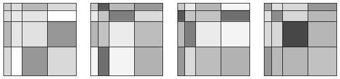
(a) Random digraphon $\mathbf{W}$ drawn from the di-IRM with $\boldsymbol{\beta}=(1,1,1,1)$

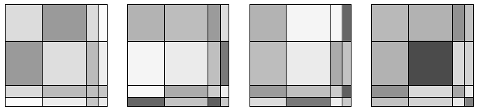
(b) Inferred weights $\boldsymbol{\eta}$, drawn in proportion to cluster sizes

(c) Sampled order

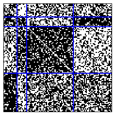
(d) True clusters

(e) Inferred clusters

Figure 10: (a) A random digraphon $\mathbf{W}$ sampled from the di-IRM; (b) the inferred weights $\boldsymbol{\eta}$; (c) a digraph sampled from $\mathbb{G}(100,\mathbf{W})$; (d) the sample sorted by increasing $U_{i}$, with true clusters shown via blue lines; (e) the sample sorted by the inferred clusters.

7 Experiments

In this section, we experimentally evaluate the di-IRM model on synthetic data. We present two examples: the first is meant to illustrate the correct behavior of inference on di-IRM parameters, and the second is designed to show the advantage of using a digraphon representation (given by the di-IRM) over using an asymmetric function (given by the IRM).

Multiple digraphons may induce the same distribution on exchangeable digraphs, in which case they are said to be weakly isomorphic. This is not just because a digraphon can be perturbed on a measure-zero set without changing the induced distribution on digraphs, but also because measurable rearrangements of the digraphon will also leave the distribution invariant (analogously to how relabeling the vertices of a digraph does not change it up to isomorphism). Hence a digraphon $\mathbf{W}$ is not identifiable from the random digraph $\mathbb{G}({{\mathbb{N}}},\mathbf{W})$; in general only its weak isomorphism class can be determined. For details (in the analogous setting of graphons), see Diaconis and Janson (2008, §7) and Orbanz and Roy (2015, §3.4).

Therefore, in the following inference problems, we can only expect to estimate a digraphon up to its weak isomorphism class. In a block model, this results in the nonidentifiability of the order of the blocks.

7.1 Random di-IRM from uniform weights

We first draw a random di-IRM $\mathbf{W}$ with the weights $\boldsymbol{\beta}=(1,1,1,1)$, which is displayed in Figure 10(a). We then generate a 100-vertex sample from this digraphon (Figure 10(c)). We ran a collapsed Gibbs sampling procedure for 200 iterations, beginning from a random initial clustering. This inference procedure is able to recover the original weights, up to reordering; the inferred weight matrices are displayed in Figure 10, drawn in proportion to the inferred cluster sizes.

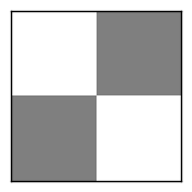
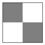
(a) Half-undirected, half-tournament digraphon $W_{00},W_{01},W_{10},W_{11}$

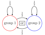
(b) Schematic of example

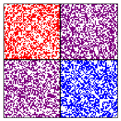
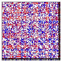
(c) left: Sample; middle: Sample reordered by di-IRM clusters (true clusters are colored), right: Sample reordered by IRM clusters

Figure 11: Half-undirected, half-tournament block model example. In the schematic, arrows show the probability of connecting in that direction; i.e., any two distinct vertices in the same group have probability $\nicefrac{{1}}{{2}}$ of an arrow in both directions (and $\nicefrac{{1}}{{2}}$ of an arrow in neither direction), while for any vertex from group $1$ and vertex from group $2$, either there is just an arrow from the first to the second, or there is just an arrow from the second to the first, each occurring with probability $\nicefrac{{1}}{{2}}$. The bottom right shows the random sample from the digraphon and the results of collapsed Gibbs sampling in the di-IRM and the IRM. White indicates no edge, red indicates an edge between vertices from group 1, blue indicates an edge between vertices from group 2, and purple indicates an edge between vertices from different groups. Black lines indicate the inferred partition.

7.2 Half-undirected, half-tournament example

We consider the 2-class step-function digraphon with half the vertices in each class that is given by $w=0$,

$$W_{00}(x,y)=W_{11}(x,y)=\begin{cases}\nicefrac{{1}}{{2}}&\text{~{}if~{}}x<\nicefrac{{1}}{{2}}\text{~{}and~{}}y<\nicefrac{{1}}{{2}},\\ \nicefrac{{1}}{{2}}&\text{~{}if~{}}x\geq\nicefrac{{1}}{{2}}\text{~{}and~{}}y\geq\nicefrac{{1}}{{2}},\\ 0&\text{~{}otherwise,}\end{cases}$$

and

$$W_{01}(x,y)=W_{10}(x,y)=\begin{cases}\nicefrac{{1}}{{2}}&\text{~{}if~{}}x\geq\nicefrac{{1}}{{2}}\text{~{}and~{}}y<\nicefrac{{1}}{{2}},\\ \nicefrac{{1}}{{2}}&\text{~{}if~{}}x<\nicefrac{{1}}{{2}}\text{~{}and~{}}y\geq\nicefrac{{1}}{{2}},\\ 0&\text{~{}otherwise.}\end{cases}$$

This digraphon is displayed in Figure 11(a), and a schematic illustrating the model is in Figure 11(b). This example demonstrates the importance of being able to distinguish regions having different correlations between edge directions (but the same marginal left-to-right and right-to-left edge probabilities).

We generated a synthetic digraph sampled from $\mathbb{G}(100,\mathbf{W})$ and then ran a collapsed Gibbs sampling procedure for the di-IRM. We also ran a similar collapsed Gibbs sampler for the IRM. Both samplers began with a random clustering and ran until the cluster assignments approximately converged. The results are shown in Figure 11(c); here the random sample is displayed alongside the sample resorted according the clusters inferred using the di-IRM model, as well as the clusters inferred by the IRM model. In both resorted images, the true clusters are colored, white indicates no edge, red indicates an edge between vertices from group 1, blue indicates an edge between vertices from group 2, and purple indicates an edge between vertices from different groups. Note that the true clusters are correctly inferred using the di-IRM model, as reordering the vertices according to the inferred clusters identifies the true groups, while the IRM model fails to discern the correct structure. The IRM only considers the marginal left-to-right and right-to-left edge probabilities, which do not distinguish the two clusters; in this particular inference run, almost all vertices were put into the first of the two clusters, which is consistent with not being able to distinguish between vertices with similar marginal edge probabilities. This result is what one would expect from an algorithm that has inferred uniform independent edge probabilities, i.e., the edge probabilities of an Erdős–Rényi graph.

8 Discussion

We have described how priors on digraphons can be used in the statistical modeling of exchangeable dense digraphs, and have exhibited several key classes of structures that one can model with particular subclasses of these priors. We have also illustrated why merely using asymmetric measurable functions is insufficient, as this produces a misspecified model for any exchangeable digraphs having correlations between the edge directions.

While models based on digraphons (and graphons) are almost surely dense (or empty) and not directly suitable for real-world network applications that are sparse, it is still useful to study models using digraphons (see, e.g., the discussion in Orbanz and Roy (2015, §7.1)). Some recent work, e.g., Borgs et al. (2015); Veitch and Roy (2015); Borgs et al. (2016); Herlau and Schmidt (2016); Cai et al. (2016); Crane and Dempsey (2016); Caron and Fox (2014), has pointed to methods for extending exchangeable graphs to the case of sparse graphs, but many interesting problems remain.

References

- Airoldi et al. (2008) E. M. Airoldi, D. M. Blei, S. E. Fienberg, and E. P. Xing. Mixed membership stochastic blockmodels. J. Machine Learning Res., 9:1981–2014, 2008.
- Aldous (1981) D. J. Aldous. Representations for partially exchangeable arrays of random variables. J. Multivariate Anal., 11(4):581–598, 1981.
- Aldous (1985) D. J. Aldous. Exchangeability and related topics. In École d’été de probabilités de Saint-Flour, XIII—1983, volume 1117 of Lecture Notes in Math., pages 1–198. Springer, Berlin, 1985.
- Alon and Shapira (2004) N. Alon and A. Shapira. Testing subgraphs in directed graphs. J. Comput. System Sci., 69(3):353–382, 2004.
- Aroskar and Cummings (2014) A. Aroskar and J. Cummings. Limits, regularity and removal for finite structures. To appear in J. Symb. Logic. ArXiv e-print 1412.8084, 2014.
- Aroskar (2012) A. Aroskar. Limits, regularity and removal for relational and weighted structures. PhD thesis, Carnegie Mellon University, 2012.
- Austin (2008) T. Austin. On exchangeable random variables and the statistics of large graphs and hypergraphs. Probab. Surv., 5:80–145, 2008.
- Blundell et al. (2012) C. Blundell, K. A. Heller, and J. M. Beck. Modelling reciprocating relationships with Hawkes processes. In Adv. Neural Inform. Process. Syst. (NIPS) 26, pages 2609–2617, 2012.
- Borgs et al. (2015) C. Borgs, J. T. Chayes, H. Cohn, and S. Ganguly. Consistent nonparametric estimation for heavy-tailed sparse graphs. ArXiv e-print 1508.06675v2, 2015.
- Borgs et al. (2016) C. Borgs, J. T. Chayes, H. Cohn, and N. Holden. Sparse exchangeable graphs and their limits via graphon processes. ArXiv e-print 1601.07134, 2016.
- Bradley and Terry (1952) R. A. Bradley and M. E. Terry. Rank analysis of incomplete block designs. I. The method of paired comparisons. Biometrika, 39:324–345, 1952.
- Cai et al. (2016) D. Cai, T. Campbell, and T. Broderick. Edge-exchangeable graphs and sparsity. In Adv. Neural Inform. Process. Syst. (NIPS) 29, 2016.
- Caron and Fox (2014) F. Caron and E. B. Fox. Sparse graphs using exchangeable random measures. ArXiv e-print 1401.1137, 2014.
- Chan and Airoldi (2014) S. H. Chan and E. Airoldi. A consistent histogram estimator for exchangeable graph models. In Proc. 31st Int. Conf. Mach. Learn. (ICML), pages 208–216, 2014.
- Chatterjee and Mukherjee (2016) S. Chatterjee and S. Mukherjee. On estimation in tournaments and graphs under monotonicity constraints. ArXiv e-print 1603.04556, 2016.
- Chatterjee (2015) S. Chatterjee. Matrix estimation by universal singular value thresholding. Ann. Statist., 43(1):177–214, 2015.
- Chung and Graham (1991) F. R. K. Chung and R. L. Graham. Quasi-random tournaments. J. Graph Theory, 15(2):173–198, 1991.
- Compton (1988) K. J. Compton. The computational complexity of asymptotic problems. I. Partial orders. Inform. and Comput., 78(2):108–123, 1988.
- Crane and Dempsey (2016) H. Crane and W. Dempsey. Edge exchangeable models for network data. ArXiv e-print 1603.04571, 2016.