Direct calculation of hadronic light-by-light scattering

Abstract:

We report calculations of hadronic light-by-light scattering amplitudes via lattice QCD evaluation of Euclidean four-point functions of vector currents. These initial results include only the fully quark-connected contribution. Particular attention is given to the case of forward scattering, which can be related via dispersion relations to the $\gamma^{*}\gamma^{*}\to\text{hadrons}$ cross section, and thus allows lattice data to be compared with phenomenology. We also present a strategy for computing the hadronic light-by-light contribution to the muon anomalous magnetic moment.

1 Introduction

The anomalous magnetic moment of the muon, $a_{\mu}\equiv(\frac{g-2}{2})_{\mu}$, is one of the most precise tests of the Standard Model. Current values from experiment and theory are

$$a_{\mu}=\begin{cases}116592089(63)\times 10^{-11}&\text{experiment~{}\cite[cite]{[\@@bibref{}{Agashe:2014kda,Bennett:2006fi}{}{}]}}\\ 116591790(65)\times 10^{-11}&\text{theory~{}\cite[cite]{[\@@bibref{}{Jegerlehner:2009ry}{}{}]}}\end{cases},$$ (1)

which disagree by three standard deviations. Upcoming experiments at Fermilab [4] and J-PARC [5] plan to reduce the experimental uncertainty by a factor of four or better, which motivates efforts to similarly reduce the theoretical uncertainty.

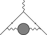
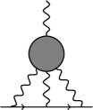
Figure 1: Leading-order contributions from the hadronic vacuum polarization (left) and hadronic light-by-light scattering (right) to $a_{\mu}$.

The leading sources of theoretical uncertainty are hadronic contributions: diagrams that include hadronic vacuum polarization and hadronic light-by-light (HLbL) scattering (Fig. 1). The former can be determined using $e^{+}e^{-}\to\text{ hadrons}$ cross sections measured in experiments, whereas current predictions for the latter rely on models. Thus, a reliable ab initio calculation of the HLbL contribution using lattice QCD would be useful for solidifying the Standard Model prediction of $a_{\mu}$. The first such calculations were done using non-perturbative lattice QCD+QED by Blum et al. [6]. In this work we take a different route of computing the HLbL amplitudes using non-perturbative lattice QCD; our plan is to combine this with continuum perturbative QED to evaluate the two-loop integrals and obtain the contribution to the muon $g-2$.

Our method provides an opportunity to study the HLbL scattering amplitude by itself. It could be used to compare lattice calculations against phenomenology and provide an independent check of the lattice methods. Conversely, it could be used for testing models used for computing $a_{\mu}^{\text{HLbL}}$ by comparing them against QCD calculations in a wide range of kinematics.

2 Lattice evaluation of the four-point function

With Wilson-type quarks, using the local and conserved vector currents, and the contact operator,

$$J_{\mu}^{l}(x) =Z_{V}\bar{q}(x)\gamma_{\mu}q(x)$$ (2)

$$J_{\mu}^{c}(x) =\frac{1}{2}\left[\bar{q}(x+\hat{\mu})(\gamma_{\mu}+1)U_{\mu}^{\dagger}(x)q(x)+\bar{q}(x)(\gamma_{\mu}-1)U_{\mu}(x)q(x+\hat{\mu})\right]$$

$$T_{\mu}(x) =\frac{1}{2}\left[\bar{q}(x+\hat{\mu})(\gamma_{\mu}+1)U_{\mu}^{\dagger}(x)q(x)-\bar{q}(x)(\gamma_{\mu}-1)U_{\mu}(x)q(x+\hat{\mu})\right]$$

we compute the local-conserved-conserved-conserved four-point function. In position space:

$$\Pi^{\text{pos}}_{\mu_{1}\mu_{2}\mu_{3}\mu_{4}}(x_{1},x_{2},0,x_{4}) =\Bigl{\langle}J_{\mu_{3}}^{l}(0)\Bigl{[}J_{\mu_{1}}^{c}(x_{1})J_{\mu_{2}}^{c}(x_{2})J_{\mu_{4}}^{c}(x_{4})+\delta_{\mu_{1}\mu_{2}}\delta_{x_{1}x_{2}}T_{\mu_{1}}(x_{1})J_{\mu_{4}}^{c}(x_{4})$$ (3)

$$\qquad+\delta_{\mu_{1}\mu_{4}}\delta_{x_{1}x_{4}}T_{\mu_{4}}(x_{4})J_{\mu_{2}}^{c}(x_{2})+\delta_{\mu_{2}\mu_{4}}\delta_{x_{2}x_{4}}T_{\mu_{4}}(x_{4})J_{\mu_{1}}^{c}(x_{1})$$

$$\qquad+\delta_{\mu_{1}\mu_{4}}\delta_{\mu_{2}\mu_{4}}\delta_{x_{1}x_{4}}\delta_{x_{2}x_{4}}J_{\mu_{4}}^{c}(x_{4})\Bigr{]}\Bigr{\rangle},$$

where the contact terms ensure that this satisfies the conserved-current Ward identities using the backward lattice derivative $\Delta$,

$$\Delta_{\mu_{1}}^{x_{1}}\Pi^{\text{pos}}_{\mu_{1}\mu_{2}\mu_{3}\mu_{4}}=\Delta_{\mu_{2}}^{x_{2}}\Pi^{\text{pos}}_{\mu_{1}\mu_{2}\mu_{3}\mu_{4}}=\Delta_{\mu_{4}}^{x_{4}}\Pi^{\text{pos}}_{\mu_{1}\mu_{2}\mu_{3}\mu_{4}}=0.$$ (4)

In our implementation, we have verified that these hold on each gauge configuration.

Figure 2: The five classes of quark contractions for four-point functions. In this work, we compute only the leftmost, fully-connected set of contractions.

There are five classes of quark contractions (Fig. 2) required to evaluate the four-point function. We evaluate only the fully-connected ones, with fixed kernels summed over $x_{1}$ and $x_{2}$:

$$\Pi^{\text{pos}^{\prime}}_{\mu_{1}\mu_{2}\mu_{3}\mu_{4}}(x_{4};f_{1},f_{2})=\sum_{x_{1},x_{2}}f_{1}(x_{2})f_{2}(x_{2})\Pi^{\text{pos}}_{\mu_{1}\mu_{2}\mu_{3}\mu_{4}}(x_{1},x_{2},0,x_{4}).$$ (5)

Using fixed kernels allows this to be evaluated using the combination of a point-source propagator from the origin, and single- and double-sequential propagators that contain one or both of the kernels. If we define $\mathcal{J}_{\mu}(x)$ and $\mathcal{T}_{\mu}(x)$ to be the point-split insertions in Eq. (2), then these three kinds of propagators are

$$\begin{gathered}S_{0}(x)\equiv S(x,0),\quad S_{f\mu}\equiv S\left[\sum_{x}f(x)\mathcal{J}_{\mu}(x)S_{0}\right],\\ S_{f\mu;g\nu}\equiv S\left[\sum_{x}f(x)\mathcal{J}_{\mu}(x)S_{g\nu}+\sum_{x}g(x)\mathcal{J}_{\nu}(x)S_{f\mu}+\delta_{\mu\nu}\sum_{x}f(x)g(x)\mathcal{T}_{\mu}(x)S_{0}\right],\end{gathered}$$ (6)

and, noting that $\mathcal{J}_{\mu}(x)$ is $\gamma_{5}$-antihermitian and $\mathcal{T}_{\mu}(x)$ is $\gamma_{5}$-hermitian, the connected four-point function is obtained as

$$\Pi^{\text{pos}^{\prime},\text{conn}}_{\mu_{1}\mu_{2}\mu_{3}\mu_{4}}(x_{4};f_{1},f_{2}) =-\Bigl{\langle}\operatorname{Tr}\Bigl{(}\gamma_{\mu_{3}}\gamma_{5}\Bigl{[}S_{f_{1}^{*}\mu_{1};f_{2}^{*}\mu_{2}}^{\dagger}\gamma_{5}\mathcal{J}_{\mu_{4}}(x_{4})S_{0}+S_{0}^{\dagger}\gamma_{5}\mathcal{J}_{\mu_{4}}(x_{4})S_{f_{1}\mu_{1};f_{2};\mu_{2}}$$ (7)

$$\qquad\qquad-S^{\dagger}_{f_{2}^{*}\mu_{2}}\gamma_{5}\mathcal{J}_{\mu_{4}}(x_{4})S_{f_{1}\mu_{1}}-S^{\dagger}_{f_{1}^{*}\mu_{1}}\gamma_{5}\mathcal{J}_{\mu_{4}}(x_{4})S_{f_{2}\mu_{2}}$$

$$\qquad\qquad+\delta_{\mu_{1}\mu_{4}}f_{1}(x_{4})\bigl{(}S_{0}^{\dagger}\gamma_{5}\mathcal{T}_{\mu_{4}}(x_{4})S_{f_{2}\mu_{2}}-S_{f_{2}^{*}\mu_{2}}^{\dagger}\gamma_{5}\mathcal{T}_{\mu_{4}}(x_{4})S_{0}\bigr{)}$$

$$\qquad\qquad+\delta_{\mu_{2}\mu_{4}}f_{2}(x_{4})\bigl{(}S_{0}^{\dagger}\gamma_{5}\mathcal{T}_{\mu_{4}}(x_{4})S_{f_{1}\mu_{1}}-S_{f_{1}^{*}\mu_{1}}^{\dagger}\gamma_{5}\mathcal{T}_{\mu_{4}}(x_{4})S_{0}\bigr{)}$$

$$\qquad\qquad+\delta_{\mu_{1}\mu_{4}}\delta_{\mu_{2}\mu_{4}}f_{1}(x_{4})f_{2}(x_{4})S_{0}^{\dagger}\gamma_{5}\mathcal{J}_{\mu_{4}}(x_{4})S_{0}\Bigr{]}\Bigr{)}\Bigr{\rangle}.$$

Generically, this requires one point-source propagator $S_{0}$, sixteen sequential propagators $S_{f\mu}$, $f\in\{f_{1},f_{2},f_{1}^{*},f_{2}^{*}\}$, and thirty-two double-sequential propagators $S_{f_{1}\mu;f_{2}\nu}$ and $S_{f_{1}^{*}\mu;f_{2}^{*}\nu}$, for a total of 49 propagators, although this number can be reduced in various special cases.

Finally, we obtain the momentum-space Euclidean four-point function using plane waves:

$$\Pi^{E}_{\mu_{1}\mu_{2}\mu_{3}\mu_{4}}(p_{4};p_{1},p_{2})=\sum_{x_{4}}e^{-ip_{4}\cdot(x_{4}+\frac{a}{2}\hat{\mu}_{4})}\Pi^{\text{pos}^{\prime}}_{\mu_{1}\mu_{2}\mu_{3}\mu_{4}}(x_{4};f_{1},f_{2})\Bigr{|}_{f_{j}(x)=e^{-ip_{j}\cdot(x+\frac{a}{2}\hat{\mu}_{j})}}.$$ (8)

Thus, by fixing $p_{1}$ and $p_{2}$ we can efficiently compute this for all $p_{4}$.

3 Lattice results

We use three ensembles with $N_{f}=2$, $O(a)$-improved Wilson fermions from CLS [8]. These have $a=0.063$ fm and pion masses between 277 and 451 MeV. We keep only $u$ and $d$ quarks in the electromagnetic current, so that in the above we actually use $J_{\mu}^{l}=\frac{2}{3}\bar{u}\gamma_{\mu}u-\frac{1}{3}\bar{d}\gamma_{\mu}d$, etc, which amounts to applying an overall factor of $\frac{17}{81}$ to the fully-connected four-point function for a single light quark. For the results shown here, relatively few statistics were needed to obtain a reasonable signal, and we used a maximum of 300 samples on each ensemble.

The four-point function is a rather complicated object, and we focus on the simplified case of forward kinematics ($p_{1}=-p_{2}$) where there are only three kinematic invariants. We take the amplitude for forward scattering of transversely polarized virtual photons,

$$\mathcal{M}_{TT}(-Q_{1}^{2},-Q_{2}^{2},\nu)=\frac{e^{4}}{4}R_{\mu_{1}\mu_{2}}R_{\mu_{3}\mu_{4}}\Pi^{E}_{\mu_{1}\mu_{2}\mu_{3}\mu_{4}}(-Q_{2};-Q_{1},Q_{1}),$$ (9)

where $\nu\equiv-Q_{1}\cdot Q_{2}$ and

$$R_{\mu\nu}\equiv\delta_{\mu\nu}-\frac{1}{(Q_{1}\cdot Q_{2})^{2}-Q_{1}^{2}Q_{2}^{2}}\left[(Q_{1}\cdot Q_{2})(Q_{1\mu}Q_{2\nu}+Q_{1\nu}Q_{2\mu})-Q_{1}^{2}Q_{2\mu}Q_{2\nu}-Q_{2}^{2}Q_{1\mu}Q_{1\nu}\right]$$ (10)

is a projector onto the plane orthogonal to $Q_{1}$ and $Q_{2}$. At fixed spacelike $Q_{1}^{2}$ and $Q_{2}^{2}$, this is related via a subtracted dispersion relation to the helicity 0 and 2 cross sections for $\gamma^{*}\gamma^{*}\to\text{hadrons}$, $\sigma_{0}$ and $\sigma_{2}$ [9]:

$$\mathcal{M}_{TT}(-Q_{1}^{2},-Q_{2}^{2},\nu)-\mathcal{M}_{TT}(-Q_{1}^{2},-Q_{2}^{2},0)=\frac{2\nu^{2}}{\pi}\int_{\nu_{0}}^{\infty}d\nu^{\prime}\frac{\sqrt{\nu^{\prime 2}-Q_{1}^{2}Q_{2}^{2}}}{\nu^{\prime}(\nu^{\prime 2}-\nu^{2}-i\epsilon)}\left[\sigma_{0}(\nu^{\prime})+\sigma_{2}(\nu^{\prime})\right],$$ (11)

where $\nu_{0}$ denotes the hadron-production threshold. By itself, this relation is model-independent. As inputs from experiment improve and the lattice calculations become more physical, this will allow for systematically improved comparisons between lattice and experiment. For now, we use a phenomenological model [9, 7] for $\sigma_{0}+\sigma_{2}$, based on single-meson and non-resonant $\pi^{+}\pi^{-}$ final states.

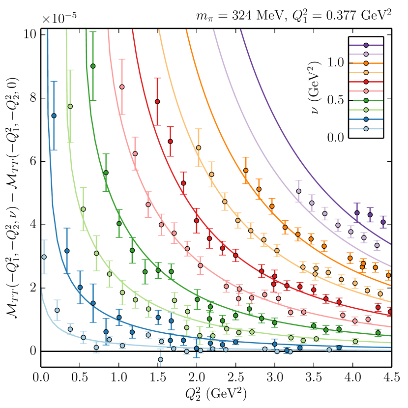
Figure 3: Forward scattering amplitude $\mathcal{M}_{TT}$ versus $Q_{2}^{2}$, for fixed $Q_{1}^{2}$ and pion mass, and a range of $\nu$. The points are lattice data and the curves result from applying the dispersion relation [Eq. (11)] to the model for the $\gamma^{*}\gamma^{*}\to\text{hadrons}$ cross section.

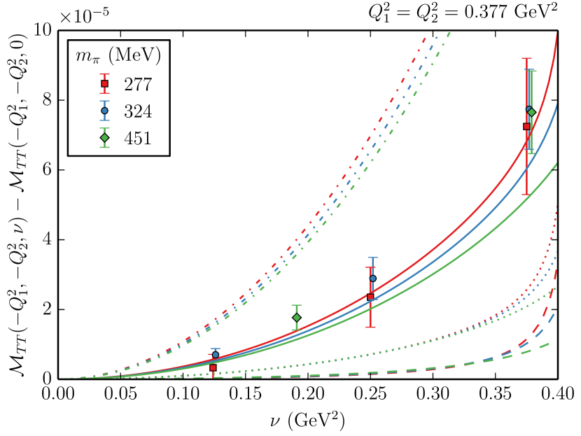
Figure 4: Forward scattering amplitude $\mathcal{M}_{TT}$ versus $\nu$, for fixed $Q_{1}^{2}$ and $Q_{2}^{2}$, and three different pion masses. The points are lattice data and the solid curves result from applying the dispersion relation [Eq. (11)] to the model for the $\gamma^{*}\gamma^{*}\to\text{hadrons}$ cross section. The dashed and dotted curves show the contributions from $\pi^{0}$ and $\pi^{0}+\eta^{\prime}$, and the dash-dotted curves include an additional high-energy Regge contribution to the cross section for the case of real photons at the physical pion mass.

We show a comparison of lattice data and the result from applying the dispersion relation to our model in Figs. 4 and 4. Figure 4 shows the wide range of $(Q_{2}^{2},\nu)$ accessible in a single calculation at fixed $Q_{1}^{2}=0.377\text{ GeV}^{2}$ and pion mass 324 MeV. The model produces good agreement with the data, although it has a considerable uncertainty. In particular, there is no data from experiment constraining the two-photon transition form factors for scalar and tensor mesons. We take this to be of the form $F(Q_{1}^{2},Q_{2}^{2})=\prod_{i=1,2}1/(1+Q_{i}^{2}/\Lambda^{2})$ and set $\Lambda$ by hand to 1.6 GeV to produce the nice agreement with our data; however, varying $\Lambda$ by $\pm 0.4$ GeV causes the curves to change by up to $\pm 50\%$.

In Fig. 4, we fix both photon virtualities to $0.377\text{ GeV}^{2}$ and show the dependence of $\mathcal{M}_{TT}$ on $\nu$, for three different pion masses. We find no significant dependence on the pion mass. The figure also shows the contributions from $\pi^{0}$ and $\eta^{\prime}$ final states in the model, which are far from being the dominant contributions. In order to see the dominance of the $\pi^{0}$ contribution, which is expected for $a_{\mu}^{\text{HLbL}}$, we may need to reach much smaller photon virtualities and closer-to-physical pion masses. Finally, we show in the figure a high-energy contribution to the $\gamma\gamma\to\text{hadrons}$ cross section, which is obtained using a fit to data based on Regge theory. This is not included in the main model due to the lack of an extrapolation to heavier-than-physical pion masses and nonzero photon virtualities, but is an indication of possible additional uncertainty in the model.

4 Strategy for evaluation of the HLbL contribution to the muon $\mathbf{g-2}$

In Euclidean space, we put the muon on shell with momentum $p=im\hat{\epsilon}$ in an arbitrary direction $\hat{\epsilon}$ ($\hat{\epsilon}^{2}=1$). Applying infinite-volume continuum QED Feynman rules to evaluate the diagram in Fig. 1 (right) and then isolating the electromagnetic form factor $F_{2}(0)$ for the muon, we obtain an expression of the form

$$a_{\mu}^{\text{HLbL}}=\int d^{4}x\,d^{4}y\,\mathcal{L}_{[\rho,\sigma];\mu\nu\lambda}(\hat{\epsilon},x,y)i\hat{\Pi}_{\rho;\mu\nu\lambda\sigma}(x,y),$$ (12)

where $\mathcal{L}$ is a kernel involving muon and photon propagators, and

$$\hat{\Pi}_{\rho;\mu\nu\lambda\sigma}(x_{1},x_{2})=\int d^{4}x_{4}\,(ix_{4})_{\rho}\langle J_{\mu}(x_{1})J_{\nu}(x_{2})J_{\lambda}(0)J_{\sigma}(x_{4})\rangle$$ (13)

is the four-point function with a momentum derivative applied to the vertex that couples to the external photon. After contracting $\mathcal{L}$ with $\hat{\Pi}$, the integrand for $a_{\mu}^{\text{HLbL}}$ is a scalar function and thus depends only on the five invariants $x^{2}$, $y^{2}$, $x\cdot y$, $x\cdot\hat{\epsilon}$, and $y\cdot\hat{\epsilon}$; therefore, three of the eight dimensions in the integral are trivial. The dimensionality can be further reduced by noting that the result is independent of $\hat{\epsilon}$, which we can therefore eliminate by averaging in the integrand. If we replace

$$\mathcal{L}(\hat{\epsilon},x,y)\to\overline{\mathcal{L}}(x,y)\equiv\langle\mathcal{L}(\hat{\epsilon},x,y)\rangle_{\hat{\epsilon}},$$ (14)

then the integrand will only depend on $x^{2}$, $y^{2}$, and $x\cdot y$.

Putting the ingredients together, we arrive at our formula:

$$a_{\mu}^{\text{HLbL}}=2\pi^{2}\int_{0}^{\infty}|x|^{3}d|x|\int d^{4}y\,d^{4}z\,\overline{\mathcal{L}}_{[\rho,\sigma];\mu\nu\lambda}(x,y)(-z)_{\rho}\langle J_{\mu}(x)J_{\nu}(y)J_{\lambda}(0)J_{\sigma}(z)\rangle,$$ (15)

where we have used the fact that, after integrating over $y$ and $z$, the integrand depends only on $x^{2}$ so that the integral over $x$ can be reduced to one dimension. We plan to compute the integrals over $y$ and $z$ similarly to our computation of the momentum-space four-point function. First, we will use local currents at $0$ and $x$, and compute point-source propagators from those points. Next, we will implement the integral over $z$ using sequential propagators with conserved-current insertions, and obtain $\hat{\Pi}(x,y)$ at all points $y$. We will then contract it with $\overline{\mathcal{L}}(x,y)$ to integrate over $y$. These steps will have a similar cost to our previous evaluation of the scattering amplitude with two of the momenta fixed. Finally, we will repeat the process several times to perform the one-dimensional integral over $|x|$.

5 Summary and outlook

We have shown that the contribution from the fully quark-connected four-point function to the HLbL scattering amplitude can be efficiently evaluated on the lattice if two of the three momenta are fixed. In the case of forward scattering, this amplitude is related model-independently by a dispersion relation to the $\gamma^{*}\gamma^{*}\to\text{hadrons}$ cross section. Using a model for the latter, we found that our lattice results are consistent with phenomenology, within the large model uncertainties. For typical Euclidean kinematics, we do not find a dominant contribution from neutral pion exchange.

Our strategy for computing the leading-order HLbL contribution to the muon $g-2$ is in place; work is ongoing to evaluate the kernel $\overline{\mathcal{L}}_{[\rho,\sigma];\mu\nu\lambda}(x,y)$. Since several model calculations [3, 10, 11] indicate that neutral pion exchange is the leading contribution to $a_{\mu}^{\text{HLbL}}$, it may be challenging to reach the physical regime on the lattice — near-physical pion masses and large volumes may be called for. In addition, disconnected diagrams may be important, as Ref. [11] argues that omitting them will lead to an unphysical enhanced $\pi^{0}$ contribution appearing instead of the $\eta^{\prime}$ contribution.

Finally, we also note the recent computation of the connected contribution to $a_{\mu}^{\text{HLbL}}$ using non-perturbative lattice QCD and perturbative lattice QED [12].

References

• [1] Particle Data Group Collaboration, K. A. Olive et al., Review of Particle Physics, Chin. Phys. C 38 (2014) 090001.
• [2] Muon g-2 Collaboration, G. W. Bennett et al., Final Report of the Muon E821 Anomalous Magnetic Moment Measurement at BNL, Phys. Rev. D 73 (2006) 072003 [hep-ex/0602035].
• [3] F. Jegerlehner and A. Nyffeler, The Muon g-2, Phys. Rept. 477 (2009) 1–110 [0902.3360].
• [4] Muon g-2 Collaboration, G. Venanzoni, The New Muon g-2 experiment at Fermilab, in International Conference on High Energy Physics 2014 (ICHEP 2014) Valencia, Spain, July 2-9, 2014. 1411.2555.
• [5] J-PARC g-2 Collaboration, T. Mibe, Measurement of muon g-2 and EDM with an ultra-cold muon beam at J-PARC, Nucl. Phys. Proc. Suppl. 218 (2011) 242–246.
• [6] T. Blum, S. Chowdhury, M. Hayakawa and T. Izubuchi, Hadronic light-by-light scattering contribution to the muon anomalous magnetic moment from lattice QCD, Phys. Rev. Lett. 114 (2015) 012001 [1407.2923].
• [7] J. Green, O. Gryniuk, G. von Hippel, H. B. Meyer and V. Pascalutsa, Lattice QCD calculation of hadronic light-by-light scattering, 1507.01577.
• [8] P. Fritzsch, F. Knechtli, B. Leder, M. Marinkovic, S. Schaefer, R. Sommer and F. Virotta, The strange quark mass and Lambda parameter of two flavor QCD, Nucl. Phys. B 865 (2012) 397–429 [1205.5380].
• [9] V. Pascalutsa, V. Pauk and M. Vanderhaeghen, Light-by-light scattering sum rules constraining meson transition form factors, Phys. Rev. D 85 (2012) 116001 [1204.0740].
• [10] V. Pauk and M. Vanderhaeghen, Single meson contributions to the muon‘s anomalous magnetic moment, Eur. Phys. J. C 74 (2014) 3008 [1401.0832].
• [11] J. Bijnens, Hadronic light-by-light contribution to $a_{\mu}$: extended Nambu-Jona-Lasinio, chiral quark models and chiral Lagrangians, in Workshop on Flavour changing and conserving processes 2015 (FCCP2015) Anacapri, Capri Island, Italy, September 10-12, 2015. 1510.05796.
• [12] T. Blum, N. Christ, M. Hayakawa, T. Izubuchi, L. Jin and C. Lehner, Lattice Calculation of Hadronic Light-by-Light Contribution to the Muon Anomalous Magnetic Moment, 1510.07100.
• [13] SciDAC, LHPC, UKQCD Collaboration, R. G. Edwards and B. Joó, The Chroma software system for lattice QCD, Nucl. Phys. Proc. Suppl. 140 (2005) 832 [hep-lat/0409003].
• [14] M. Lüscher, S. Schaefer et al., “openQCD.” http://luscher.web.cern.ch/luscher/openQCD/.