Flexibly Mining Better Subgroups

Abstract

In subgroup discovery, also known as supervised pattern mining, discovering high quality one-dimensional subgroups and refinements of these is a crucial task. For nominal attributes, this is relatively straightforward, as we can consider individual attribute values as binary features. For numerical attributes, the task is more challenging as individual numeric values are not reliable statistics. Instead, we can consider combinations of adjacent values, i.e. bins. Existing binning strategies, however, are not tailored for subgroup discovery. That is, they do not directly optimize for the quality of subgroups, therewith potentially degrading the mining result.

To address this issue, we propose flexi. In short, with flexi we propose to use optimal binning to find high quality binary features for both numeric and ordinal attributes. We instantiate flexi with various quality measures and show how to achieve efficiency accordingly. Experiments on both synthetic and real-world data sets show that flexi outperforms state of the art with up to 25 times improvement in subgroup quality.

1 Introduction

Subgroup discovery aims at finding subsets of the data, called subgroups, with high statistical unusualness with respect to the distribution of target variable(s) [23, 7, 5]. It has applications in many areas, e.g. spatial analysis [7], marketing campaign management [9], and health care [13].

A crucial part of the subgroup discovery process is the extraction of high quality binary features out of existing attributes. By binary features, we mean features whose values are either true or false. For instance, possible binary features of Age attribute are Age $\geq 50$ and $20\leq$ Age $\leq 30$. These features constitute one-dimensional subgroups or one-dimensional refinements of subgroups, which are used by many existing search schemes (e.g. beam search) [6, 20, 2].

Deriving such features is straightforward for nominal attributes, e.g. their individual values can be used directly as binary features [12]. This also is the case for ordinal attributes if one is to treat them as nominal; the downside is that their ordinal nature is not used. The task, however, becomes more challenging for numerical (e.g. real-valued) attributes. For such an attribute, binary features formed by single values statistically and empirically are not reliable; they tend to have low generality. Thus, one usually switches to combinations of adjacent values, i.e. bins.

To this end, we observe three challenges that are in the way of finding high quality bins, i.e. binary features, for subgroup discovery. First, we need a problem formulation tailored to this purpose. Commonly used binning strategies such as equal-width and equal-frequency are oblivious of subgroup quality, impacting quality of the final output. Second, we should not place any restriction on the target; be it univariate or multivariate; nominal, ordinal, or numeric. Existing solutions also do not address this issue. For instance, sd [3] used in [5] requires that the target is univariate and nominal. Likewise, roc [12] requires a univariate target. Third, the solution should scale well in order to handle large data sets. This means that we need new methods that can handle the first two issues and are efficient.

In this paper, we aim at tackling these challenges. We do so by proposing flexi, for flexible subgroup discovery. In short, flexi formulates the search of binary features per numeric/ordinal attribute as identifying the features with maximal average quality. This formulation meets the generality requirement since it does not make any assumption on the target. We instantiate flexi with various quality measures and show how to achieve efficiency accordingly. Extensive experiments on large real-world data sets show that flexi outperforms state of the art, providing up to 25 times improvement in terms of subgroup quality. Furthermore, flexi scales very well on large data sets.

The road map of this paper is as follows. In Section 2, we present preliminaries. In Section 3, we introduce flexi. In Sections 4 and 5, we plug different quality measures into our method and explain how to achieve efficiency. In Section 6, we review related work. We present the experimental results in Section 7. In Section 8 we round up with a discussion and conclude the paper in Section 9. For readability, we put all proofs in the appendix.

2 Preliminaries

Let us consider a data set $\mathbf{D}$ of size $m$ with attributes $\mathbf{A}=\{A_{1},\ldots,A_{n}\}$, and targets $\mathbf{T}=\{T_{1},\ldots,T_{d}\}$. Each attribute $A\in\mathbf{A}$ can be nominal, ordinal, or numeric. When $A$ is either nominal or ordinal, its domain $\mathit{dom}(A)$ is the set of its possible values. Each target $T\in\mathbf{T}$ can be either numeric or ordinal. If $T_{i}\in\mathbf{T}$ is numeric, we assume that $\mathit{dom}(T_{i})=[\mathit{v}_{i},\mathit{V}_{i}]$. Otherwise, $\mathit{dom}(T_{i})$ is the set of possible values of $T_{i}$. The probability function of $\mathbf{T}$ on $\mathbf{D}$ is denoted as $p(\mathbf{T})$.

A subgroup $\mathit{S}$ on $\mathbf{D}$ has the form $b_{1}\wedge\ldots\wedge b_{k}$ ($k\in[1,n]$) where (1) each $b_{j}$ ($j\in[1,k]$) is a condition imposed on some attribute $A\in\mathbf{A}$ and (2) no two conditions share the same attribute. For each numeric attribute $A$, each of its conditions $b$ has the form $A\in(l,u]$ where $l\in\mathbb{R}\cup\{-\infty\}$, $u\in\mathbb{R}\cup\{+\infty\}$, and $l<u$. If $A$ is ordinal, $b$ also has the form $A\in(l,u]$ where $l,u\in\mathit{dom}(A)$ and $l<u$. If $A$ is categoric, $b$ instead has the form $A=a$ where $a\in\mathit{dom}(A)$.

We let $\mathcal{S}$ be the set of all subgroups on $\mathbf{D}$. The subset of $\mathbf{D}$ covered by $\mathit{S}$ is denoted as $\mathbf{D}_{\mathit{S}}$. We write $p_{\mathit{S}}(\mathbf{T})$ as the probability function of $\mathbf{T}$ on $\mathbf{D}_{\mathit{S}}$. Overall, subgroup discovery is concerned with detecting $\mathit{S}$ having high exception in its target distribution. The level of exception can be expressed through the divergence between $p_{\mathit{S}}(\mathbf{T})$ and $p(\mathbf{T})$. To achieve high generality – besides the divergence score – the support $s=|\mathbf{D}_{\mathit{S}}|$ of $\mathit{S}$ should not be too small.

To quantify quality of subgroups, we need quality measure $\phi:\mathcal{S}\rightarrow\mathbb{R}$ which assigns a score to each subgroup; the higher the score the better. Typically, $\phi$ needs to capture both unusualness of target distribution and subgroup support. In this paper, we will study five such quality measures.

3 Mining Binary Features

flexi mines binary features for attribute $A$ that is either numeric or ordinal. When the features serve as one-dimensional subgroups on the first level of the search lattice, the entire realizations of $A$ are used. For one-dimensional refinements, only those realizations covered by the subgroup in consideration are used [20, 13]. For readability, we keep our discussion to the first case. The presentation can straightforwardly be adapted to the second case by switching from the context of the entire data set $\mathbf{D}$ to its subset covered by the subgroup to be refined. Below we also use bins and binary features interchangeably.

In a nutshell, flexi aims at finding binary features with maximal average quality. More specifically, it searches for the binning $\mathit{dsc}$ of $A$ such that the average quality of the bins formed by $\mathit{dsc}$ is maximal. Formally, let $\mathcal{F}$ be the set of possible binnings on $A$. For each $g\in\mathcal{F}$, we let $\{b_{g}^{1},\ldots,b_{g}^{|g|}\}$ be the set of bins formed by $g$ where $|g|$ is its number of bins. Each bin $b_{g}^{i}=(l_{g}^{i},u_{g}^{i}]$ where $l_{g}^{1}=-\infty$, $u_{g}^{|g|}=+\infty$, and $l_{g}^{i}=u_{g}^{i-1}$ for $i\in[2,|g|]$. flexi solves for

$$\textstyle\mathit{dsc}=\arg\max\limits_{g\in\mathcal{F}}\frac{1}{|g|}\sum\limits_{i=1}^{|g|}\phi(b_{g}^{i}).$$

Another alternative would be to consider the sum of subgroup quality. We discuss this option shortly afterward. Now, we present flexi, our solution to the above problem.

At first, we note that $|\mathcal{F}|=O(2^{m})$, i.e. the search space is exponential in $m$ making an exhaustive enumeration infeasible. Fortunately, it is structured. In particular, for each $\lambda\in[1,m]$ let $\mathit{dsc}_{\lambda}$ be the optimal solution over all binnings producing $\lambda$ bins on $A$. Let $\{b_{\mathit{dsc}}^{1},\ldots,b_{\mathit{dsc}}^{\lambda}\}$ be its bins. We observe that for a fixed value of $\lambda$,

(3.1) $$\textstyle\sum\limits_{i=1}^{\lambda}\phi(b_{\mathit{dsc}}^{i})=\phi(b_{\mathit{dsc}}^{\lambda})+\sum\limits_{i=1}^{\lambda-1}\phi(b_{\mathit{dsc}}^{i})$$

must be maximal. On the other hand, as $\mathit{dsc}_{\lambda}$ is optimal w.r.t. $\lambda$, $\{b_{\mathit{dsc}}^{1},\ldots,b_{\mathit{dsc}}^{\lambda-1}\}$ must be the optimal way to partition values $A\leq l_{\mathit{dsc}}^{\lambda}$ into $\lambda-1$ bins. Otherwise, we could have chosen a better way to do so. This consequently would produce another binning for all values of $A$ such that (1) this binning has $\lambda$ bins and (2) it has a total quality higher than that of $\mathit{dsc}_{\lambda}$. The existence of such a binning contradicts our assumption on $\mathit{dsc}_{\lambda}$.

Hence, for each $\lambda$ its optimal binning $\mathit{dsc}_{\lambda}$ exhibits optimal substructure. This motivates us to build a dynamic programming algorithm to solve our problem.

Algorithmic approach. Our flexi solution is in Algorithm 1. In short, it first forms bins $\{c_{1},\ldots,c_{\beta}\}$ where $\beta\ll m$. Each value $\mathit{qual}[\lambda][i]$ where $\lambda\in[1,\beta]$ and $i\in[\lambda,\beta]$ stands for the total quality of bins obtained by optimally merging (discretizing) initial bins $c_{1},\ldots,c_{i}$ into $\lambda$ bins. $b[\lambda][i]$ contains the resulting bins. Our goal is to efficiently compute $\mathit{qual}[1\ldots\beta][\beta]$ and $b[1\ldots\beta][\beta]$. To do so, from Lines 4 to 6 we first compute $\mathit{qual}[1][1\ldots\beta]$ and $b[1][1\ldots\beta]$. Then from Lines 7 to 14, we incrementally compute relevant elements of arrays $\mathit{qual}$ and $b$, using the recursive relation described in Equation (3.1). This is standard dynamic programming. Finally, we return the optimal binning after normalizing by the number of bins (Lines 15 and 16). There are two important points to note here.

First, we form initial bins $\{c_{1},\ldots,c_{\beta}\}$ of $A$. Ideally, one would start with $O(m)$ bins. However, the quality score $\phi(c)$ of bin $c$ is not reliable as well as not meaningful when its support $|c|=O(1)$. Thus, by pre-partitioning $A$ in to $\beta$ bins, we ensure that there is sufficient data in each bin for a statistically reliable assessment of divergence. Choosing a suitable value for $\beta$ represents a tradeoff between accuracy and efficiency. We empirically study its effect in Section 7.

Second, to ensure efficiency we need an efficient strategy to pre-compute $\phi(\bigcup_{k=j}^{i}c_{k})$ (used in Lines 5, 9, and 10) for all $1\leq j\leq i\leq\beta$. In the next section, we explain how to do this for different quality measures and analyze the complexity of flexi accordingly.

Algorithm 1 flexi

1:  Create initial disjoint bins $\{c_{1},\ldots,c_{\beta}\}$ of $A$

2:  Create a double array $\mathit{qual}[1\ldots\beta][1\ldots\beta]$

3:  Create an array $b[1\ldots\beta][1\ldots\beta]$ to store bins

4:  for $i=1\rightarrow\beta$ do

5:     $b[1][i]=\bigcup_{k=1}^{i}c_{k}$ and $\mathit{qual}[1][i]=\phi(b[1][i])$

6:  end for

7:  for $\lambda=2\rightarrow\beta$ do

8:     for $i=\lambda\rightarrow\beta$ do

9:        $\mathit{pos}=\arg\max\limits_{1\leq j\leq i-1}\mathit{qual}[\lambda-1][j]+\phi(\bigcup_{k=j+1}^{i}c_{k})$

10:        $\mathit{qual}[\lambda][i]=\mathit{qual}[\lambda-1][\mathit{pos}]+\phi(\bigcup_{k=\mathit{pos}+1}^{i}c_{k})$

11:        Copy all bins in $b[\lambda-1][\mathit{pos}]$ to $b[\lambda][i]$

12:        Add $\bigcup_{k=\mathit{pos}+1}^{i}c_{k}$ to $b[\lambda][i]$

13:     end for

14:  end for

15:  $\lambda^{*}=\arg\max\limits_{1\leq\lambda\leq\beta}\frac{1}{\lambda}\mathit{qual}[\lambda][\beta]$

16:  Return $b[\lambda^{*}][\beta]$

Alternative setting. An intuitive alternate formulation of the problem is to maximize the total quality of 1-D subgroups formed on $A$. Formally, we have $\mathit{dsc}=\arg\max\limits_{g\in\mathcal{F}}\sum\limits_{i=1}^{|g|}\phi(b_{g}^{i})$, which can also be solved by dynamic programming (see Appendix A for details). We compare to this setting in the experiments. We find that our standard setting, maximizing the average score, leads to much better results.

4 Quality Measures

flexi works with any quality measure. In this section we show how to achieve efficiency, i.e. efficiently pre-compute $\phi(\bigcup_{k=j}^{i}c_{k})$ for all $1\leq j\leq i\leq\beta$, with various measures handling different types of targets. More specifically, we look at five measures: $\mathit{WRAcc}$ [5, 4, 20], $\mathit{z\textit{-}score}$ [12], a measure based on Kullback-Leibler divergence ($\mathit{kl}$) [20, 21], a measure based on Hellinger distance ($\mathit{hd}$) [10], and a measure based on quadratic measure of divergence ($\mathit{qr}$) [14]. We show characteristics of all measures in Table 1 and provide their details below. To simplify our analysis, we assume that each bin $c_{i}$ ($i\in[1,\beta]$) contains $\frac{m}{\beta}$ objects.

	Univariate				Multivariate
Measure	Nominal	Ordinal	Numeric		Nominal	Ordinal	Numeric
$\mathit{WRAcc}$	✓	✓	✗		✗	✗	✗
$\mathit{z\textit{-}score}$	✗	✗	✓		✗	✗	✗
$\mathit{kl}$	✓	✓	✗		✓	✓	✗
$\mathit{hd}$	✓	✓	✗		✓	✓	✗
$\mathit{qr}$	✗	✓	✓		✗	✓	✓

Table 1: Characteristics of quality measures considered in this paper.

4.1 $\mathit{WRAcc}$ measure

In subgroup discovery this measure is suited when $\mathbf{D}$ has a single binary target $T$. That is, $T$ assumes either a positive or a negative nominal value. Let $m_{+}$ be the number of objects in $\mathbf{D}$ having positive target, i.e. positive label. Consider a subgroup $\mathit{S}$ having $s=|\mathbf{D}_{\mathit{S}}|$ objects; $s_{+}$ of which have positive label. The $\mathit{WRAcc}$ score of $\mathit{S}$ is defined as

$$\textstyle\mathit{WRAcc}(\mathit{S})=\frac{s}{m}(\frac{s_{+}}{s}-\frac{m_{+}}{m}).$$

Algorithm 2 shows how to pre-compute $\mathit{WRAcc}(\bigcup_{k=j}^{i}c_{k})$ for all $1\leq j\leq i\leq\beta$. The first for loop (Lines 2 to 5) is to count the number of positively labeled objects of $c_{i}$ ($i\in[1,\beta]$) and hence compute its $\mathit{WRAcc}$ score. This step takes $O(m)$. The nested loop (Lines 6 to 12) is to incrementally count the number of positively labeled objects of $\bigcup_{k=j}^{i}c_{k}$ and hence compute its $\mathit{WRAcc}$ score. This step takes $O(\beta^{2})$. Thus, Algorithm 2 takes $O(m+\beta^{2})$.

Hence, flexi with $\mathit{WRAcc}$ measure (flexi_w) takes $O(m+\beta^{2}+\beta^{3})=O(m+\beta^{3})$.

Algorithm 2 Pre-computation with $\mathit{WRAcc}$

1:  Create an integer array $\mathit{countPos}[1\ldots\beta]$

2:  for $i=1\rightarrow\beta$ do

3:     $\mathit{countPos}[i]=$ # of objects in $\mathbf{D}_{c_{i}}$ with positive label

4:     Compute $\mathit{WRAcc}(c_{i})$ based on $\mathit{countPos}[i]$

5:  end for

6:  for $i=2\rightarrow\beta$ do

7:     $\theta=\mathit{countPos}[i]$

8:     for $j=i-1\rightarrow 1$ do

9:        $\theta=\theta+\mathit{countPos}[j]$

10:        Set # of objects with positive label in $\bigcup_{k=j}^{i}c_{k}$ to $\theta$ and hence compute $\mathit{WRAcc}(\bigcup_{k=j}^{i}c_{k})$

11:     end for

12:  end for

4.2 $\mathit{z\textit{-}score}$ measure

This measure is suited when $\mathbf{D}$ has a single numeric target $T$. Let $\mu_{0}$ and $\sigma_{0}$ be the mean and standard deviation of $T$ in $\mathbf{D}$. Consider a subgroup $\mathit{S}$ and let $\mu$ and $\sigma$ be the mean and standard deviation of $T$ in $\mathit{S}$. The quality of $\mathit{S}$ w.r.t. $\mathit{z\textit{-}score}$ is defined as

$$\textstyle\mathit{z\textit{-}score}(\mathit{S})=\frac{\sqrt{s}}{\sigma_{0}}(\mu-\mu_{0})$$

where $s=|\mathbf{D}_{\mathit{S}}|$. To pre-compute $\mathit{z\textit{-}score}(\bigcup_{k=j}^{i}c_{k})$ for all $1\leq j\leq i\leq\beta$, we can re-use Algorithm 2 with a few modifications. The new algorithm is in Algorithm 3. It also takes $O(m+\beta^{2})$.

Hence, flexi with $\mathit{z\textit{-}score}$ measure (flexi_z) has the same complexity as flexi_w.

Algorithm 3 Pre-computation with $\mathit{z\textit{-}score}$

1:  Create an integer array $\mathit{binMean}[1\ldots\beta]$

2:  for $i=1\rightarrow\beta$ do

3:     $\mathit{binMean}[i]=$ target mean in $c_{i}$

4:     Compute $\mathit{z\textit{-}score}(c_{i})$ based on $\mathit{binMean}[i]$

5:  end for

6:  for $i=2\rightarrow\beta$ do

7:     $\theta=|c_{i}|$

8:     $\mu=\mathit{binMean}[i]$

9:     for $j=i-1\rightarrow 1$ do

10:        $\mu=\theta\times\mu+|c_{j}|\times\mathit{binMean}[j]$

11:        $\theta=\theta+|c_{j}|$

12:        Set target mean in $\bigcup_{k=j}^{i}c_{k}$ to $\mu$ and hence compute $\mathit{z\textit{-}score}(\bigcup_{k=j}^{i}c_{k})$

13:     end for

14:  end for

4.3 $\mathit{kl}$ measure

This measure is suited to $\mathbf{D}$ with univariate/multivariate nominal and/or ordinal target. W.l.o.g., assume that we have multivariate target $\mathbf{T}=\{T_{1},\ldots,T_{d}\}$. The $\mathit{kl}$ score of each subgroup $\mathit{S}$ is defined as

$$\textstyle\mathit{kl}(\mathit{S})=\frac{s}{m}\sum\limits_{t_{1},\ldots,t_{d}}p_{\mathit{S}}(t_{1},\ldots,t_{d})\times\log\frac{p_{\mathit{S}}(t_{1},\ldots,t_{d})}{p(t_{1},\ldots,t_{d})}$$

where $s=|\mathbf{D}_{\mathit{S}}|$. A straightforward computation of $\mathit{kl}(\bigcup_{k=j}^{i}c_{k})$ for every $1\leq j\leq i\leq\beta$ is done by considering only $(t_{1},\ldots,t_{d})$ that appears in the data covered by $\mathit{S}$. This is because $p_{\mathit{S}}(t_{1},\ldots,t_{d})\times\log\frac{p_{\mathit{S}}(t_{1},\ldots,t_{d})}{p(t_{1},\ldots,t_{d})}=0$ for $(t_{1},\ldots,t_{d})$ not in $\mathit{S}$. As $p_{\mathit{S}}(t_{1},\ldots,t_{d})$ and $p(t_{1},\ldots,t_{d})$ can be efficiently calculated using hash tables, computing $\mathit{kl}(\bigcup_{k=j}^{i}c_{k})$ takes $O((i-j+1)\times d\times\frac{m}{\beta})$. The pre-computation hence in total takes

$$\textstyle\sum\limits_{i=1}^{\beta}\sum\limits_{j=1}^{i}O((i-j+1)\times d\times\frac{m}{\beta}),$$

which can be simplified to $O(m\beta^{2}d)$.

Thus, flexi with $\mathit{kl}$ (flexi_k) takes $O(m\beta^{2}d+\beta^{3})=O(m\beta^{2}d)$ as $\beta\ll m$.

4.4 $\mathit{hd}$ measure

Similarly to $\mathit{kl}$ measure, $\mathit{hd}$ measure is suited to $\mathbf{D}$ with univariate/multivariate nominal and/or ordinal target. The $\mathit{hd}$ score of a subgroup $\mathit{S}$ is defined as

$$\textstyle\mathit{hd}(\mathit{S})=\left(-\frac{s}{m}\log\frac{s}{m}-\frac{m-s}{m}\log\frac{m-s}{m}\right)$$

$$\textstyle\quad\quad\times\sum\limits_{t_{1},\ldots,t_{d}}\left(\sqrt{p_{\mathit{S}}(t_{1},\ldots,t_{d})}-\sqrt{p(t_{1},\ldots,t_{d})}\right)^{2}.$$

where $s=|\mathbf{D}_{\mathit{S}}|$. The pre-computation is done similarly to Section 4.3. However, we here need to consider $(t_{1},\ldots,t_{d})$ that appears in $\mathbf{D}$, not just in $\mathit{S}$. Thus, for $(i,j)$ where $j\leq i$, computing $\mathit{hd}(\bigcup_{k=j}^{i}c_{k})$ takes $O(md)$. Hence, the cost of the pre-computation is identical to that of flexi_k.

In other words, flexi with $\mathit{hd}$ measure (flexi_h) has the same complexity as flexi_k.

4.5 $\mathit{qr}$ measure

To handle univariate/multivariate numeric and/or ordinal targets, we propose $\mathit{qr}$ measure which is based on $\mathit{ID}$ – a quadratic measure of divergence [14]. We pick $\mathit{ID}$ as it is applicable to both univariate and multivariate data. In addition, its computation on empirical data is in closed form formula, i.e. it is highly suited to exploratory data analysis. Originally, $\mathit{ID}$ is used for numeric data. Our $\mathit{qr}$ measure improves over this by adapting $\mathit{ID}$ to ordinal data. This enables $\mathit{qr}$ to handle multivariate numeric targets, as well as multivariate targets whose types are a mixed of numeric and ordinal. As shown in Table 1, no previous measure is able to achieve this. By making $\mathit{qr}$ work with flexi, we can further demonstrate the flexibility and generality of our solution. The details are as follows.

Consider a subgroup $\mathit{S}$ with $s=|\mathbf{D}_{\mathit{S}}|$ objects. W.l.o.g., assume that there are multiple targets. The $\mathit{qr}$ score of $\mathit{S}$ is

$$\textstyle\mathit{qr}(\mathit{S})=f(s)\times\mathit{ID}(p_{\mathit{S}}(\mathbf{T})\;||\;p(\mathbf{T}))$$

where $f(s)$ is either $\frac{s}{m}$ (following [5, 21]) or $\left(\frac{s}{m}\log\frac{s}{m}-\frac{m-s}{m}\log\frac{m-s}{m}\right)$ (following [10, 2]). When all targets are numeric, we have $\mathit{ID}(p_{\mathit{S}}(\mathbf{T})\;||\;p(\mathbf{T}))=$

$$\textstyle\int_{\mathit{v}_{1}}^{\mathit{V}_{1}}\cdots\int_{\mathit{v}_{d}}^{\mathit{V}_{d}}\left(P_{\mathit{S}}(t_{1},\ldots,t_{d})-P(t_{1},\ldots,t_{d})\right)^{2}dt_{1}\cdots dt_{d}$$

where $P_{\mathit{S}}(.)$ and $P(.)$ are the cdfs of $p_{\mathit{S}}(.)$ and $p(.)$, respectively. We extend to ordinal targets by replacing $\int_{\mathit{v}_{i}}^{\mathit{V}_{i}}dt_{i}$ with $\sum\limits_{t_{i}\in\mathit{dom}(T_{i})}$ for each ordinal $T_{i}$.

Similarly to $\mathit{ID}$, our $\mathit{qr}$ measure also permits computation on empirical data in closed form. More specifically, let the empirical data of $\mathbf{D}$ be $\{\mathbf{D}^{1},\ldots,\mathbf{D}^{m}\}$. Similarly, let the empirical data of $\mathbf{D}_{\mathit{S}}$ be $\{\mathbf{D}_{\mathit{S}}^{1},\ldots,\mathbf{D}_{\mathit{S}}^{s}\}$ where $s=|\mathbf{D}_{\mathit{S}}|$. We write $\mathbf{D}^{1}_{i}$ and $\mathbf{D}_{\mathit{S},i}^{1}$ as the projections of $\mathbf{D}^{1}$ and respectively $\mathbf{D}_{\mathit{S}}^{1}$ on $T_{i}$. We have the following.

Theorem 4.1

Empirically, $\mathit{qr}(p_{\mathit{S}}(\mathbf{T})\;||\;p(\mathbf{T}))=$

$$\textstyle f(s)\times\left(\frac{1}{s^{2}}\sum\limits_{i=1}^{s}\sum\limits_{j=1}^{s}\prod\limits_{k=1}^{d}h_{k}(\mathbf{D}_{\mathit{S},i}^{k},\mathbf{D}_{\mathit{S},j}^{k})\right.$$

$$\left.\textstyle\qquad\qquad-\frac{2}{sm}\sum\limits_{i=1}^{s}\sum\limits_{j=1}^{m}\prod\limits_{k=1}^{d}h_{k}(\mathbf{D}_{\mathit{S},i}^{k},\mathbf{D}_{j}^{k})\right.$$

$$\left.\textstyle\qquad\qquad+\frac{1}{m^{2}}\sum\limits_{i=1}^{m}\sum\limits_{j=1}^{m}\prod\limits_{k=1}^{d}h_{k}(\mathbf{D}_{i}^{k},\mathbf{D}_{j}^{k})\right)$$

where $h_{k}\left(x,y\right)=\left(\mathit{V}_{k}-\max(x,y)\right)$ if $T_{k}$ is numeric, and $h_{k}\left(x,y\right)=\sum\limits_{t\in\mathit{dom}(T_{k})}\textbf{I}\left(t\geq\max(x,y)\right)$ if $T_{k}$ is ordinal. Here, $\textbf{I}(.)$ is an indicator function.

• We postpone the proof to Appendix B.

Following Theorem 4.1, to obtain $\mathit{qr}(p_{\mathit{S}}(\mathbf{T})\;||\;p(\mathbf{T}))$ we need to compute three terms – referred to as $\mathit{S}.e_{1}$, $\mathit{S}.e_{2}$, and $\mathit{S}.e_{3}$ – where

$$\textstyle\mathit{qr}(p_{\mathit{S}}(\mathbf{T})\;||\;p(\mathbf{T}))=f(s)\times\left(\frac{1}{s^{2}}\mathit{S}.e_{1}-\frac{2}{sm}\mathit{S}.e_{2}+\frac{1}{m^{2}}\mathit{S}.e_{3}\right).$$

Note that $e=\mathit{S}.e_{3}$ is independent of $\mathit{S}$ and thus needs to be computed only once for all subgroups. We now prove a property of $\mathit{qr}$ which is important for efficiently pre-computing $\mathit{qr}(\bigcup_{k=j}^{i}c_{k})$ for all $1\leq j\leq i\leq\beta$.

Lemma 4.1

Let $\mathit{S}$ and $\mathit{R}$ be two consecutive non-overlapping bins of attribute $A$, i.e. $\mathbf{D}_{\mathit{S}}\cap\mathbf{D}_{\mathit{R}}=\emptyset$. Let $Y=\mathit{S}\cup\mathit{R}$, $s=|\mathbf{D}_{\mathit{S}}|$, and $r=|\mathbf{D}_{\mathit{R}}|$. It holds that $Y.e_{1}=\mathit{S}.e_{1}+\mathit{R}.e_{1}+2\mathit{int}(\mathit{S},\mathit{R})$ and $Y.e_{2}=\mathit{S}.e_{2}+\mathit{R}.e_{2}$ where $\mathit{int}(\mathit{S},\mathit{R})=\sum\limits_{i=1}^{s}\sum\limits_{j=1}^{r}\prod\limits_{k=1}^{d}h_{k}(\mathbf{D}_{\mathit{S},i}^{k},\mathbf{D}_{\mathit{R},j}^{k})$.

• We postpone the proof to Appendix B.

Lemma 4.1 tells us that terms $e_{1}$ and $e_{2}$ of a bin made up by joining two adjacent non-overlapping bins $S$ and $R$ can be obtained from the terms of $S$ and $R$, and $\mathit{int}(\mathit{S},\mathit{R})$. Note that $\mathit{int}$ is symmetric. Further, we prove that it is additive – a property that is also important for the pre-computation.

Lemma 4.2

Let $\mathit{R}_{1},\ldots,\mathit{R}_{l}$, and $\mathit{S}$ be non-overlapping bins of $A$ such that $\mathit{R}_{i}$ is adjacent to $\mathit{R}_{i+1}$ for $i\in[1,l-1]$, and $\mathit{R}_{l}$ is adjacent to $\mathit{S}$. It holds that

$$\textstyle\mathit{int}\left(\mathit{S},\bigcup_{i=1}^{l}\mathit{R}_{i}\right)=\sum\limits_{i=1}^{l}\mathit{int}(\mathit{S},\mathit{R}_{i}).$$

• We postpone the proof to Appendix B.

Algorithm 4 summarizes how to compute $\mathit{qr}(\bigcup_{k=j}^{i}c_{k})$ for all $1\leq j\leq i\leq\beta$. The details are as follows.

• First, we compute terms $e_{1}$ and $e_{2}$, and $\mathit{qr}(c_{i})$ for each $i\in[1,\beta]$ (Line 1): This step takes $O(m\times\frac{m}{\beta}\times d)$ for each $c_{i}$, i.e. its total cost is $O(m^{2}d)$.

• Second, we compute $\mathit{int}(c_{j},c_{i})$ for each $j\in[1,\beta-1]$ and $i\in[j+1,\beta]$ (Line 2): This step takes $O(\frac{m^{2}}{\beta^{2}}d)$ for each pair $(j,i)$, i.e. its total cost is $O(m^{2}d)$.

• Third, we compute $\mathit{int}(\bigcup_{k=j}^{i-1}c_{k},c_{i})$ for each $i\in[2,\beta]$ and $j\in[1,i-1]$ (Lines 3 to 9): We use the fact that $\mathit{int}(\bigcup_{k=j}^{i-1}c_{k},c_{i})=\sum_{k=j}^{i-1}\mathit{int}(c_{k},c_{i})$ (see Lemma 4.2). This step takes $O(\beta^{2})$.

• Fourth, we compute terms $e_{1}$ and $e_{2}$, and $\mathit{qr}(\bigcup_{k=j}^{i}c_{k})$ for each $i\in[2,\beta]$ and $j\in[1,i-1]$ (Lines 10 to 14): From Lemma 4.1, terms $e_{1}$ and $e_{2}$ of $\bigcup_{k=j}^{i}c_{k}$ can be computed based on the terms of $\bigcup_{k=j}^{i-1}c_{k}$, $c_{i}$, and $\mathit{int}(\bigcup_{k=j}^{i-1}c_{k},c_{i})$. This step takes $O(\beta^{2})$.

Overall, Algorithm 4 takes $O(m^{2}d)$. Thus, flexi with $\mathit{qr}$ (flexi_q) takes $O(m^{2}d+\beta^{3})=O(m^{2}d)$ as $\beta\ll m$.

Algorithm 4 Pre-computation with $\mathit{qr}$

1:  Compute terms $e_{1}$ and $e_{2}$, and $\mathit{qr}(c_{i})$ for $c_{i}$ ($i\in[1,\beta]$)

2:  Compute $\mathit{int}(c_{j},c_{i})$ for every $j\in[1,\beta-1]$ and $i\in[j+1,\beta]$

3:  for $i=2\rightarrow\beta$ do

4:     $\theta=0$

5:     for $j=i-1\rightarrow 1$ do

6:        $\theta=\theta+\mathit{int}(c_{j},c_{i})$

7:        Set $\mathit{int}(\bigcup_{k=j}^{i-1}c_{k},c_{i})$ to $\theta$

8:     end for

9:  end for

10:  for $i=2\rightarrow\beta$ do

11:     for $j=1\rightarrow i-1$ do

12:        Compute terms $e_{1}$ and $e_{2}$, and $\mathit{qr}(\bigcup_{k=j}^{i}c_{k})$ for $\bigcup_{k=j}^{i}c_{k}$ using the terms of $\bigcup_{k=j}^{i-1}c_{k}$, $c_{i}$, and $\mathit{int}(\bigcup_{k=j}^{i-1}c_{k},c_{i})$

13:     end for

14:  end for

4.6 Remarks

As $\beta$ is typically small (from 5 to 40), flexi_w, flexi_z, flexi_k, and flexi_h scale linearly in $m$. On the other hand, flexi_q scales quadratic in $m$ regardless which value $\beta$ takes. In Section 5, we propose a method to boost the efficiency of flexi_q.

5 Improving Scalability

The complexity of flexi_q is quadratic in $m$, which may become a disadvantage on large data. We thus propose a solution to alleviate the issue. Again, we keep our discussion to the case of one-dimensional subgroups. The case of refinements straightforwardly follows.

We observe that the performance bottleneck is the pre-computations of $\mathit{qr}(c_{i})$ ($i\in[1,\beta]$) and $\mathit{int}(c_{j},c_{i})$ ($j\in[1,\beta-1]$ and $i\in[j+1,\beta]$). In fact, keys to these quantities are the distributions $p_{c_{i}}(\mathbf{T})$ in bins $c_{i}$ ($i\in[1,\beta])$. In our computation the data of $\mathbf{D}_{c_{i}}$ projected onto $\mathbf{T}$, denoted as $\mathbf{D}_{c_{i},\mathbf{T}}$, is considered to be i.i.d. samples of the (unknown) pdf $p_{c_{i}}(\mathbf{T})$. By definition, i.i.d. samples are obtained by randomly sampling from an infinite population or by randomly sampling with replacement from a finite population [19]. In both cases, the distribution of i.i.d. samples are assumed to be identical to the distribution of the population. This is especially true when the sample size is very large [18]. Thus, when $m$ is very large the size of $\mathbf{D}_{c_{i},\mathbf{T}}$ – which is $\frac{m}{\beta}$ – is also large. This makes the empirical distribution $\hat{p}_{c_{i}}(\mathbf{T})$ formed by $\mathbf{D}_{c_{i},\mathbf{T}}$ approach the true distribution $p_{c_{i}}(\mathbf{T})$.

Assume now that we randomly draw with replacement $\epsilon\times\frac{m}{\beta}$ samples $\mathbf{d}_{c_{i},\mathbf{T}}$ from $\mathbf{D}_{c_{i},\mathbf{T}}$ where $\epsilon\in(0,1)$. As mentioned above, $\mathbf{d}_{c_{i},\mathbf{T}}$ contains i.i.d. samples of $\hat{p}_{c_{i}}(\mathbf{T})\approx p_{c_{i}}(\mathbf{T})$. As with any set of i.i.d. samples with a reasonable size, we can assume that the distribution of $\mathbf{T}$ in $\mathbf{d}_{c_{i},\mathbf{T}}$ is identical to $p_{c_{i}}(\mathbf{T})$.

Based on this line of reasoning, when $m$ is large we propose to randomly subsample with replacement the data in each bin $c_{i}$ ($i\in[1,\beta]$) for our computation. The important point here is to identify how large $\epsilon$ should be, i.e. how many samples we should use. We will show that a low value of $\epsilon$ already suffices, e.g. $\epsilon=0.1$. If we subsample the bins while not subsampling $\mathbf{D}$ (in the same way) for computing quality scores, the complexity of flexi_q is $O(\epsilon m^{2}d)$. If we subsample $\mathbf{D}$ as well, its complexity is then $O(\epsilon^{2}m^{2}d)$.

6 Related Work

Traditionally, subgroup discovery focuses on nominal attributes [7, 9, 6, 4]. More recent work [20, 2, 13, 11] considers numeric attributes, employing equal-width or equal-frequency binning to create binary features. These strategies however do not optimize quality of the features generated, which consequently affects the final output quality.

To alleviate this, Grosskreutz and Rüping [5] employ sd [3]. It requires that the target is univariate and nominal. Further, it finds the bins optimizing the divergence between $p_{b}(\mathbf{T})$ and $p_{b^{\prime}}(\mathbf{T})$ where $b$ and $b^{\prime}$ are two arbitrary consecutive bins. That is, only local distributions of the target (within individual bins) are compared to each other. The goal of subgroup discovery in turn is to assess the divergence between $p_{b}(\mathbf{T})$ and $p(\mathbf{T})$ [6]. While sd improves over naïve binning methods, it does not directly optimize subgroup quality.

Mampaey et al. [12] introduce roc, which searches for the binary feature with highest quality on each numeric/ordinal attribute. It does so by analyzing the coverage space, reminiscent of ROC spaces, of the univariate target. roc and flexi are different in many aspects. First, roc is suitable for univariate targets only. flexi in turn works with both univariate and multivariate targets. Second, as roc finds the best feature per attribute, it is not for mining one-dimensional subgroups. In fact, it is designed for mining one-dimensional refinements. On the contrary, flexi can find both types of pattern. Third, roc requires $\phi$ to be convex. flexi in turn works with any type of quality measures.

Besides the binning methods discussed above, there exist also other techniques applicable to – albeit not yet studied in – subgroup discovery. For instance, ud [8] mines bins per numeric attribute that best approximate its true distribution. On the other hand, multivariate binning techniques (e.g. ipd [14]) focus on optimizing the divergence between local distributions in individual bins. Overall, these methods do not optimize subgroup quality.

Regarding quality measure $\phi$, majority of existing ones focus on univariate targets [7, 9, 6, 5, 4, 22, 12, 13, 11]. Van Leeuwen and Knobbe [20, 21] propose a measure based on Kullback-Leibler divergence for multivariate nominal/ordinal targets. Their measure is reminiscent of $\mathit{kl}$ measure in Section 4.3; yet, they assume the targets are statistically independent while $\mathit{kl}$ takes into account interaction of targets. Also for multivariate nominal/ordinal targets, Duivesteijn et al. [2] introduce a measure based on Bayesian network. Measures for multivariate numeric targets appear mainly in exceptional model mining (EMM) [10, 1]. Consequently, such measures are model-based. Our $\mathit{qr}$ measure in turn is purely non-parametric. A non-parametric measure for multivariate numeric targets is recently introduced in [16]. Unlike this measure as well as measures of EMM, $\mathit{qr}$ can handle multivariate targets whose types are a mixed of numeric and ordinal.

7 Experiments

		Attributes
Data	Rows	Nom.	Ord.	Num.	Total
Adult	48 842	7	1	6	14
Bike	17 379	5	3	7	15
Cover	581 012	44	3	7	54
Gesture	9 900	1	0	32	33
Letter	20 000	1	0	16	16
Bank	45 211	11	2	8	21
Naval	11 934	0	0	18	18
Network	53 413	1	9	14	24
SatImage	6 435	1	0	36	37
Drive	58 509	1	0	48	49
Turkiye	5 820	0	32	1	33
Year	515 345	1	0	90	91

Table 2: Characteristics of real-world data sets. ‘Nom.’, ’Ord.’, and ’Num.’ are abbreviations of respectively ‘Nominal’, ‘Ordinal’, and ‘Numerical’.

In this section, we empirically evaluate flexi by plugging it into beam search – a common search scheme of subgroup discovery [10, 20, 2]. We aim at examining if flexi is able to efficiently and effectively discover subgroups of high quality. For a comprehensive assessment, we test with all five quality measures discussed above. As performance metric, we use the average quality of top 50 subgroups. We also study the parameter setting of flexi; this includes the effect of our scalability improvement for $\mathit{qr}$ measure (see Section 5). We implemented flexi in Java, and make our code available for research purposes.​ All experiments were performed single-threaded on an Intel(R) Core(TM) i7-4600U CPU with 16GB RAM. We report wall-clock running times.

We compare flexi to sum which finds bins optimizing the sum of quality instead of average quality, ef for equal-frequency binning, and ew for equal-width binning. As further baselines, we test with state of the art supervised discretization sd [3], unsupervised univariate discretization ud [8], and unsupervised multivariate discretization ipd [14]. For measures that handle univariate targets only ($\mathit{WRAcc}$ and $\mathit{z\textit{-}score}$), we test with ud and exclude ipd. For the other three measures, we use ipd instead. Finally, we include roc [12], state of the art method on mining binary features for subgroup discovery. For each competitor, whenever applicable we try with different parameter settings and pick the best result. For flexi, by default we set the number of initial bins $\beta=20$; and when subsampling is used, we set the subsampling rate $\epsilon=0.1$. We form initial bins $\{c_{1},\ldots,c_{\beta}\}$ by applying equal-frequency binning; this procedure has also been used in [17, 14, 15].

We experiment with 12 real-world data sets drawn from the UCI Machine Learning Repository. Their details are in Table 2. To show that flexi methods are suited to subgroup discovery on large-scale data, 9 data sets we pick have more than 10 000 records. For brevity, in the following we present the results on 6 data sets with largest sizes: Adult, Cover, Bank, Network, Drive, and Year. For conciseness, we keep our discussion to flexi_w, flexi_k, and flexi_q; we postpone further results to Appendix C.

7.1 Quality results with $\mathit{WRAcc}$

As $\mathit{WRAcc}$ requires univariate binary target, we follow [13] to convert nominal (but non-binary) targets to binary. The results are in Tables 3. Here, we display the absolute as well as relative average quality (for other measures we show relative quality only). For the relative quality, the scores of flexi_w are the bases (100%). Going over the results, we see that flexi_w gives the best average quality in all data sets. Its performance gain over the competitors is up to 300%. Note that by optimizing average subgroup quality, instead of total quality as sum does, flexi_w mines better binary features and hence achieves better performance than sum. ef, ew, sd, and ud form binary features oblivious of subgroup quality and perform less well. roc, on the other hand, performs better, but as it forms one feature per attribute at each level of the search it makes the search more sensitive to local optima.

Data	flexiw	sum	ef	ew	sd	ud	roc
Adult	0.08 (100)	0.07 (88)	0.07 (88)	0.07 (88)	0.07 (88)	0.06 (75)	0.07 (88)
Cover	0.12 (100)	0.11 (92)	0.04 (33)	0.08 (66)	0.04 (33)	0.05 (42)	0.04 (33)
Bank	0.04 (100)	0.03 (75)	0.02 (50)	0.03 (75)	0.02 (50)	0.02 (50)	0.02 (50)
Network	0.18 (100)	0.13 (72)	0.10 (56)	0.12 (67)	0.14 (78)	0.12 (67)	0.14 (78)
Drive	0.11 (100)	0.08 (73)	0.03 (27)	0.08 (73)	0.05 (45)	0.06 (55)	0.05 (45)
Year	0.12 (100)	0.08 (67)	0.06 (50)	0.06 (50)	0.07 (58)	0.06 (50)	0.07 (58)

Table 3: [Higher is better] Average quality, measured by $\mathit{WRAcc}$, of top 50 subgroups. We give both the absolute scores, as well as the relative results (in brackets) compared to flexi_w.

7.2 Quality results with $\mathit{kl}$

We recall that $\mathit{kl}$ is suited to univariate/multivariate nominal and/or ordinal targets. For Adult and Bank, we use all nominal attributes as targets. For Cover, we randomly select 27 nominal attributes as targets. For Network, we combine nominal and ordinal attributes to create the targets. Drive and Year both have one nominal attribute and no ordinal one. Thus, for each of them we use the nominal attribute as univariate target.

The results are in Table 4. flexi_k achieves the best performance in all data sets. It yields up to 25 times quality improvement compared to competing methods. Note that sd and roc both require univariate targets and hence are not applicable to Adult, Cover, Bank, and Network. flexi_k in turn is suited to both univariate and multivariate targets.

Data	flexik	sum	ef	ew	sd	ipd	roc
Adult	100	38	37	31	n/a	4	n/a
Cover	100	43	64	75	n/a	45	n/a
Bank	100	46	62	33	n/a	6	n/a
Network	100	55	68	55	n/a	21	n/a
Drive	100	42	64	85	89	42	62
Year	100	43	45	42	40	42	74

Table 4: [Higher is better] Average quality, measured by $\mathit{kl}$, of top 50 subgroups. The results are relative and the quality of flexi_k on each data set is the base (100%).

7.3 Quality results with $\mathit{qr}$

We recall that $\mathit{qr}$ is suited to univariate/multivariate numeric and/or ordinal targets. In this experiment, we focus on multivariate targets; hence, sd and roc are inapplicable. Regarding the setup, for Adult we combine the ordinal attribute and two randomly selected numeric attributes to form targets. For Cover, we pick three ordinal attributes as targets. For Bank, we combine the two ordinal attributes and two randomly selected numeric attributes to create targets. For Network, we randomly sample five ordinal attributes and five numeric attributes to form targets. For Drive and Year, we randomly pick half of the numeric attributes as targets.

To avoid runtimes of more than 5 hours on Cover, Network, Drive, and Year, for all methods we subsample with $\epsilon=0.1$. Note that with ef, ew, and ipd, we need to compute subgroup quality after the bins have been formed, which in total is quadratic to the data size $m$. Thus, to ensure efficiency subsampling is also necessary. For the final subgroups, we use their actual quality for evaluation. Each quality value resulted from using subsampling is the average of 10 runs; standard deviation is small and hence skipped.

The results are in Table 5. We see that flexi_q outperforms all competitors with large margins, improving quality up to 14 times.

Data	flexiq	sum	ef	ew	ipd
Adult	100	18	7	8	23
Cover	100	60	41	39	53
Bank	100	31	47	59	66
Network	100	48	69	64	56
Drive	100	62	41	59	66
Year	100	26	27	21	55

Table 5: [Higher is better] Average quality, measured by $\mathit{qr}$, of top 50 subgroups. The results are relative and the quality of flexi_q on each data set is the base (100%).

7.4 Efficiency results

We here compare the efficiency of methods that have an advanced way to form binary features; that is, for fairness we skip ef and ew. The relative runtime of all remaining methods are shown in Figures 3(a), 3(b), and 3(c). The results of our methods in each case are the bases. We observe that we overall are faster than roc. This could be attributed to the fact that we form initial bins before mining actual features. roc in turn uses the original set of cut points and hence has a larger search space per attribute. We can also see that our methods have comparable runtime to sum. While in theory sum is more efficient than our method, it may unnecessarily form too many binary features per attribute, which potentially incurs higher runtime for the whole subgroup discovery process.

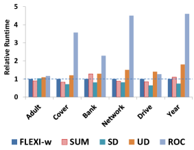
(a) Runtime with $\mathit{WRAcc}$

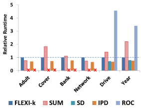
(b) Runtime with $\mathit{kl}$

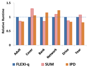
(c) Runtime with $\mathit{qr}$

Figure 1: [Lower is better] Relative runtime with $\mathit{WRAcc}$, $\mathit{kl}$, and $\mathit{qr}$. In each case the runtime of flexi is the base. sd and roc are not applicable to Adult, Cover, Bank, and Network, which is marked by ✗.

7.5 Parameter setting

flexi has two input parameters: the number of initial bins $\beta$ and the subsampling rate $\epsilon$. To assess the sensitivity to $\beta$, we vary it from 5 to 40 with step size being 5. For sensitivity to $\epsilon$, we vary it from 0.05 to 0.2 with step size being 0.05. The default setting is $\beta=20$ and $\epsilon=0.1$. The results are in Figures 2(a) and 2(b). For $\beta$, we show representative outcome of flexi_w and flexi_k on Adult and Bank. For $\epsilon$, we show outcome of flexi_q on Network and Drive. We can see that our methods are very stable to parameter setting.

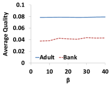
(a) Quality vs. $\beta$

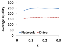
(b) Quality vs. $\epsilon$

Figure 2: Sensitivity to $\beta$ and $\epsilon$. For $\beta$, we show the results of flexi_w and flexi_k on Adult and Bank. For $\epsilon$, we show the results of flexi_q on Network and Drive.

8 Discussion

The experiments on different quality measures and real-world data sets show that flexi found subgroups of higher quality than existing methods. In terms of efficiency, it is on par with sum and faster than roc– the state of the art for mining binary features for subgroup discovery. The good performance of flexi could be attributed to (1) our formulation of binary feature mining which takes into account subgroup quality, (2) our efficient dynamic programming algorithm which searches for optimal binary features, and (3) our subsampling method to handle very large data sets.

Yet, there is room for alternative methods as well as further improvements. For instance, in addition to beam search it is also interesting to apply flexi to other search paradigms, e.g. MDL-based search [20]. Along this line, we can also formulate our search problem as mining binary features with high quality that together effectively compress the data. Besides the already demonstrated efficiency of our method, it can be further sped up by parallelization, e.g. with MapReduce. This direction in fact is applicable to subgroup discovery in general and is a potential solution towards making methods in this area more applicable to real-world scenarios.

9 Conclusion

We studied the problem of mining binary features for subgroup discovery. This is challenging as one needs a formulation that allows us to identify features leading to the detection of high quality subgroup. Second, the solution should place no restrictions on the target. Third, it should permit efficient computation. To address these issues, we proposed flexi. In short, flexi aims at identifying binary features per attribute with maximal average quality. The formulation of flexi is abstract from the targets and hence suited to any type of targets. We instantiated flexi with five different measures and showed how to make it efficient in every case. Extensive experiments on various real-world data sets verified that compared to existing methods, flexi is able to efficiently detect subgroups with considerably higher quality.

A Alternative Setting

Here we show that the alternate problem formulation can also be solved by dynamic programing. More specifically, let $\mathit{dsc}$ be the optimal solution and $\{b_{\mathit{dsc}}^{1},\ldots,b_{\mathit{dsc}}^{|\mathit{dsc}|}\}$ be its bins. It holds that

$$\sum_{i=1}^{|\mathit{dsc}|}\phi(b_{\mathit{dsc}}^{i})=\phi(b_{\mathit{dsc}}^{|\mathit{dsc}|})+\sum_{i=1}^{|\mathit{dsc}|-1}\phi(b_{\mathit{dsc}}^{i}).$$

As $\mathit{dsc}$ is optimal, $\{b_{\mathit{dsc}}^{1},\ldots,b_{\mathit{dsc}}^{|\mathit{dsc}|-1}\}$ must be the optimal binning for values $A\leq l_{\mathit{dsc}}^{|\mathit{dsc}|}$. Otherwise, we could have chosen a different binning for such values that improves the total quality. This would yield another binning for all values of $A$ that has a total quality higher than that of $\mathit{dsc}$, which contradicts the assumption on $\mathit{dsc}$. Hence, the optimal binning $\mathit{dsc}$ also exhibits optimal substructure, permitting the use of dynamic programming. The detailed solution is in Algorithm 5.

Algorithm 5 sum

1:  Create initial disjoint bins $\{c_{1},\ldots,c_{\beta}\}$ of $A$

2:  Create a double array $\mathit{qual}[1\ldots\beta]$

3:  Create an array $b[1\ldots\beta]$ whose each entry stores bins

4:  Set $\mathit{qual}[1]=\phi(c_{1})$ and $b[1]=c_{1}$

5:  for $i=2\rightarrow\beta$ do

6:     $\mathit{pos}=\arg\max\limits_{1\leq j\leq i-1}\mathit{qual}[j]+\phi(\bigcup_{k=j+1}^{i}c_{k})$

7:     $\mathit{qual}[i]=\mathit{qual}[\mathit{pos}]+\phi(\bigcup_{k=\mathit{pos}+1}^{i}c_{k})$

8:     Copy all bins in $b[\mathit{pos}]$ to $b[i]$

9:     Add $\bigcup_{k=\mathit{pos}+1}^{i}c_{k}$ to $b[i]$

10:  end for

11:  Return $b[\beta]$

B Proofs

• [Theorem 4.1] W.l.o.g., we assume that $T_{1},\ldots,T_{l}$ are numeric and $T_{l+1},\ldots,T_{d}$ are ordinal. We have

  $$P(t_{1},\ldots,t_{d})=$$

  $$\int_{\mathit{v}_{1}}^{\mathit{V}_{1}}\ldots\int_{\mathit{v}_{l}}^{\mathit{V}_{l}}\sum\limits_{t_{l+1}\in\mathit{dom}(T_{l+1})}\ldots\sum\limits_{t_{d}\in\mathit{dom}(T_{d})}\mathbf{I}(x_{1}\leq t_{1})\times$$

  $$\cdots\times\mathbf{I}(x_{d}\leq t_{d})\times p(x_{1},\ldots,x_{d})dx_{1}\cdots dx_{d}.$$

  Similarly, we have

  $$P_{\mathit{S}}(t_{1},\ldots,t_{d})=$$

  $$\int_{\mathit{v}_{1}}^{\mathit{V}_{1}}\ldots\int_{\mathit{v}_{l}}^{\mathit{V}_{l}}\sum\limits_{t_{l+1}\in\mathit{dom}(T_{l+1})}\ldots\sum\limits_{t_{d}\in\mathit{dom}(T_{d})}\mathbf{I}(x_{1}\leq t_{1})\times$$

  $$\cdots\times\mathbf{I}(x_{d}\leq t_{d})\times p_{\mathit{S}}(x_{1},\ldots,x_{d})dx_{1}\cdots dx_{d}.$$

  Using empirical data, we have

  $$P(t_{1},\ldots,t_{d})=\frac{1}{m}\sum_{i=1}^{m}\prod_{k=1}^{d}\mathbf{I}(\mathbf{D}^{i}_{k}\leq t_{i}),\quad\textrm{ and }$$

  $$P_{\mathit{S}}(t_{1},\ldots,t_{d})=\frac{1}{s}\sum_{i=1}^{s}\prod_{k=1}^{d}\mathbf{I}(\mathbf{D}^{i}_{\mathit{S},k}\leq t_{i}).$$

  Hence, we have

  $$\mathit{ID}(p_{\mathit{S}}(\mathbf{T})\;||\;p(\mathbf{T}))=$$

  $$\int_{\mathit{v}_{1}}^{\mathit{V}_{1}}\ldots\int_{\mathit{v}_{l}}^{\mathit{V}_{l}}\sum\limits_{t_{l+1}\in\mathit{dom}(T_{l+1})}\ldots\sum\limits_{t_{d}\in\mathit{dom}(T_{d})}$$

  $$\left(\frac{1}{s}\sum_{i=1}^{s}\prod_{k=1}^{d}\mathbf{I}(\mathbf{D}^{i}_{\mathit{S},k}\leq t_{i})-\frac{1}{m}\sum_{i=1}^{m}\prod_{k=1}^{d}\mathbf{I}(\mathbf{D}^{i}_{k}\leq t_{i})\right)^{2}dt_{1}\cdots dt_{l}.$$

  Expanding the above term and bringing the integrals inside the sums, we have

  $$\mathit{ID}(p_{\mathit{S}}(\mathbf{T})\;||\;p(\mathbf{T}))=$$

  $$\frac{1}{s^{2}}\sum_{i=1}^{s}\sum_{j=1}^{s}\left(\prod_{k=1}^{l}\int_{\mathit{v}_{i}}^{\mathit{V}_{i}}\mathbf{I}(\max(\mathbf{D}_{\mathit{S},k}^{i},\mathbf{D}_{\mathit{S},k}^{j})\leq t_{k})dt_{k}\right)\times$$

  $$\qquad\qquad\left(\prod_{k=l+1}^{d}\sum\limits_{t_{k}\in\mathit{dom}(T_{k})}\mathbf{I}(\max(\mathbf{D}_{\mathit{S},k}^{i},\mathbf{D}_{\mathit{S},k}^{j})\leq t_{k})\right)$$

  $$-\frac{2}{sm}\sum_{i=1}^{s}\sum_{j=1}^{m}\left(\prod_{k=1}^{l}\int_{\mathit{v}_{i}}^{\mathit{V}_{i}}\mathbf{I}(\max(\mathbf{D}_{\mathit{S},k}^{i},\mathbf{D}_{k}^{j})\leq t_{k})dt_{k}\right)\times$$

  $$\qquad\qquad\left(\prod_{k=l+1}^{d}\sum\limits_{t_{k}\in\mathit{dom}(T_{k})}\mathbf{I}(\max(\mathbf{D}_{\mathit{S},k}^{i},\mathbf{D}_{k}^{j})\leq t_{k})\right)$$

  $$+\frac{1}{m^{2}}\sum_{i=1}^{m}\sum_{j=1}^{m}\left(\prod_{k=1}^{l}\int_{\mathit{v}_{i}}^{\mathit{V}_{i}}\mathbf{I}(\max(\mathbf{D}_{k}^{i},\mathbf{D}_{k}^{j})\leq t_{k})dt_{k}\right)\times$$

  $$\qquad\qquad\left(\prod_{k=l+1}^{d}\sum\limits_{t_{k}\in\mathit{dom}(T_{k})}\mathbf{I}(\max(\mathbf{D}_{k}^{i},\mathbf{D}_{k}^{j})\leq t_{k})\right)$$

  by which we arrive at the final result.

• [Lemma 4.1] Empirically, we have that

  $$\mathit{div}(p_{\mathit{S}\cup\mathit{R}}(\mathbf{T})\;||\;p(\mathbf{T}))$$

  $$=\frac{1}{(s+r)^{2}}\sum_{i=1}^{s+r}\sum_{j=1}^{s+r}\prod_{k=1}^{d}h_{k}(\mathbf{D}_{\mathit{S}\cup\mathit{R},i}^{k},\mathbf{D}_{\mathit{S}\cup\mathit{R},j}^{k})$$

  $$-\frac{2}{(s+r)m}\sum_{i=1}^{s+r}\sum_{j=1}^{m}\prod_{k=1}^{d}h_{k}(\mathbf{D}_{\mathit{S}\cup\mathit{R},i}^{k},\mathbf{D}_{j}^{k})$$

  $$+\frac{1}{m^{2}}\sum_{i=1}^{m}\sum_{j=1}^{m}\prod_{k=1}^{d}h_{k}(\mathbf{D}_{i}^{k},\mathbf{D}_{j}^{k}).$$

  We can see that the first term is equal to $\frac{1}{(s+r)^{2}}\mathit{S}.e_{1}+\frac{1}{(s+r)^{2}}\mathit{R}.e_{1}+\frac{2}{(s+r)^{2}}\mathit{int}(\mathit{S},\mathit{R})$ where $\mathit{int}(\mathit{S},\mathit{R})=\sum\limits_{i=1}^{s}\sum\limits_{j=1}^{r}\prod\limits_{k=1}^{d}h_{k}(\mathbf{D}_{\mathit{S},i}^{k},\mathbf{D}_{\mathit{R},j}^{k})$. The second term is equal to $\frac{2}{(s+r)m}\mathit{S}.e_{2}+\frac{2}{(s+r)m}\mathit{R}.e_{2}$. The third term is in fact $e$.

• [Lemma 4.2] By definition, we have that

  $$\mathit{int}\left(\mathit{S},\bigcup_{i=1}^{l}\mathit{R}_{i}\right)$$

  $$=\sum_{q=1}^{s}\sum_{j=1}^{s_{1}+\ldots+s_{l}}\prod_{k=1}^{d}h_{k}(\mathbf{D}_{\mathit{S},q}^{k},\mathbf{D}_{\bigcup_{i=1}^{l}\mathit{R}_{i},j}^{k})$$

  $$=\sum_{i=1}^{l}\sum_{q=1}^{s}\sum_{j=1}^{s_{i}}\prod_{k=1}^{d}h_{k}(\mathbf{D}_{\mathit{S},q}^{k},\mathbf{D}_{\mathit{R}_{i},j}^{k})$$

  $$=\sum_{i=1}^{l}\mathit{int}(\mathit{S},\mathit{R}_{i}).$$

C Additional Experimental Results

Quality results on all quality measures are in Tables 6, 7, 8, 9, and 10. Note that we show absolute values. As Naval has neither categorical nor ordinal attributes, it is not applicable to $\mathit{WRAcc}$, $\mathit{kl}$, and $\mathit{hd}$.

Additional efficiency results are in Figures 3(a), 3(b), and 3(c). Interestingly, on $\mathit{qr}$ measure, flexi_q is even faster than ew on 3 data sets. Our explanation is similar to the case of sum; that is, ew may form unnecessarily many binary features than required per attribute which prolongs the runtime.

Data	flexiw	sum	ef	ew	sd	ud	roc
Adult	0.08	0.07	0.07	0.07	0.07	0.06	0.07
Bike	0.06	0.04	0.04	0.04	0.06	0.04	0.05
Cover	0.12	0.11	0.04	0.08	0.04	0.05	0.04
Gesture	0.10	0.08	0.03	0.09	0.07	0.04	0.04
Letter	0.08	0.05	0.02	0.03	0.05	0.04	0.04
Bank	0.04	0.03	0.02	0.03	0.02	0.02	0.02
Network	0.18	0.13	0.10	0.12	0.14	0.12	0.14
SatImage	0.15	0.11	0.03	0.05	0.09	0.04	0.05
Drive	0.11	0.08	0.03	0.08	0.05	0.06	0.05
Turkiye	0.11	0.11	0.10	0.10	0.10	0.10	0.10
Year	0.12	0.08	0.06	0.06	0.07	0.06	0.07
Average	0.10	0.08	0.05	0.07	0.07	0.06	0.06

Table 6: [Higher is better] Average quality, measured by $\mathit{WRAcc}$, of top 50 subgroups. Best values are in bold.

Data	flexiz	sum	ef	ew	ud	roc
Adult	89.44	82.14	82.14	86.04	79.62	82.14
Bike	68.61	50.44	57.54	50.24	56.25	61.50
Cover	434.97	328.43	356.44	249.49	288.29	384.48
Gesture	38.09	31.38	35.32	33.55	31.42	44.01
Letter	47.11	41.90	43.82	39.97	40.77	44.17
Bank	78.76	69.54	72.45	71.39	66.40	72.45
Naval	28.20	23.60	22.92	22.50	22.61	32.25
Network	135.09	129.38	133.60	114.78	110.45	145.91
SatImage	50.28	35.23	39.32	41.94	39.42	44.16
Drive	120.33	86.64	69.57	46.93	44.43	40.80
Turkiye	14.56	9.53	9.53	9.54	7.10	12.37
Year	88.57	57.59	47.93	53.50	50.40	60.31
Average	99.50	78.82	80.88	68.32	69.76	85.38

Table 7: [Higher is better] Average quality, measured by $\mathit{z\textit{-}score}$, of top 50 subgroups. Best values are in bold.

Data	flexik	sum	ef	ew	sd	ipd	roc
Adult	0.52	0.20	0.19	0.16	n/a	0.02	n/a
Bike	0.50	0.26	0.34	0.35	n/a	0.05	n/a
Cover	0.53	0.23	0.34	0.40	n/a	0.24	n/a
Gesture	0.53	0.22	0.33	0.33	0.50	0.31	0.33
Letter	0.52	0.43	0.43	0.47	0.43	0.06	0.43
Bank	0.52	0.24	0.32	0.17	n/a	0.03	n/a
Network	0.53	0.29	0.36	0.29	n/a	0.11	n/a
SatImage	0.53	0.28	0.37	0.48	0.45	0.26	0.37
Drive	0.53	0.22	0.34	0.45	0.47	0.22	0.33
Turkiye	0.53	0.50	0.50	0.50	n/a	0.15	n/a
Year	0.53	0.23	0.24	0.22	0.21	0.22	0.39
Average	0.52	0.28	0.34	0.35	0.19	0.16	0.17

Table 8: [Higher is better] Average quality, measured by $\mathit{kl}$, of top 50 subgroups. Best values are in bold.

Data	flexih	sum	ef	ew	sd	ipd	roc
Adult	0.29	0.26	0.26	0.26	n/a	0.22	n/a
Bike	0.27	0.10	0.14	0.22	n/a	0.25	n/a
Cover	0.30	0.30	0.22	0.21	n/a	0.27	n/a
Gesture	0.29	0.08	0.14	0.30	0.27	0.30	0.14
Letter	0.29	0.21	0.21	0.25	0.24	0.25	0.28
Bank	0.29	0.13	0.16	0.23	n/a	0.26	n/a
Network	0.29	0.22	0.22	0.21	n/a	0.25	n/a
SatImage	0.29	0.11	0.16	0.24	0.23	0.23	0.17
Drive	0.29	0.08	0.14	0.28	0.29	0.30	0.14
Turkiye	0.29	0.26	0.26	0.26	n/a	0.26	n/a
Year	0.29	0.25	0.12	0.14	0.14	0.22	0.15
Average	0.29	0.18	0.18	0.24	0.11	0.26	0.08

Table 9: [Higher is better] Average quality, measured by $\mathit{hd}$, of top 50 subgroups. Best values are in bold.

Data	flexiq	sum	ef	ew	ipd
Adult	110.35	20.1	8.19	8.58	25.38
Bike	1.77	0.49	0.61	0.69	0.75
Cover	185.72	110.51	76.58	71.95	98.52
Gesture	3.25	0.82	1.13	2.58	2.86
Letter	0.59	0.35	0.36	0.41	0.44
Bank	41.71	13.02	19.60	24.54	27.63
Naval	0.57	0.18	0.21	0.26	0.28
Network	25.72	12.37	17.63	16.34	14.34
SatImage	3.57	1.23	2.20	1.94	2.11
Drive	6.37	3.94	2.64	3.76	4.22
Turkiye	1.03	0.85	0.77	0.83	0.83
Year	271.98	69.41	73.07	55.95	149.43
Average	54.39	19.44	16.92	15.65	27.23

Table 10: [Higher is better] Average quality, measured by $\mathit{qr}$, of top 50 subgroups. Best values are in bold.

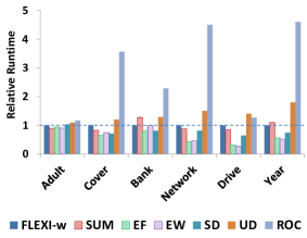
(a) Runtime with $\mathit{WRAcc}$

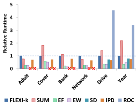
(b) Runtime with $\mathit{kl}$

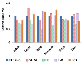
(c) Runtime with $\mathit{qr}$

Figure 3: [Lower is better] Relative runtime with $\mathit{WRAcc}$, $\mathit{kl}$, and $\mathit{qr}$. The runtime of our methods in each case is the base. sd and roc are not applicable to Adult, Cover, Bank, and Network, which is marked by ✗.

References

- [1] W. Duivesteijn, A. Feelders, and A. J. Knobbe. Different slopes for different folks: mining for exceptional regression models with cook’s distance. In KDD, pages 868–876, 2012.
- [2] W. Duivesteijn, A. J. Knobbe, A. Feelders, and M. van Leeuwen. Subgroup discovery meets bayesian networks – an exceptional model mining approach. In ICDM, pages 158–167, 2010.
- [3] U. M. Fayyad and K. B. Irani. Multi-interval discretization of continuous-valued attributes for classification learning. In IJCAI, pages 1022–1029, 1993.
- [4] H. Grosskreutz and D. Paurat. Fast and memory-efficient discovery of the top-k relevant subgroups in a reduced candidate space. In ECML/PKDD (1), pages 533–548, 2011.
- [5] H. Grosskreutz and S. Rüping. On subgroup discovery in numerical domains. Data Min. Knowl. Discov., 19(2):210–226, 2009.
- [6] H. Grosskreutz, S. Rüping, and S. Wrobel. Tight optimistic estimates for fast subgroup discovery. In ECML/PKDD (1), pages 440–456, 2008.
- [7] W. Klösgen. Advances in knowledge discovery and data mining, Chapter Explora: a multipattern and multistrategy discovery assistant. MIT Press, Cambridge, 1996.
- [8] P. Kontkanen and P. Myllymäki. MDL histogram density estimation. In AISTATS, pages 219–226, 2007.
- [9] N. Lavrac, B. Kavsek, P. A. Flach, and L. Todorovski. Subgroup discovery with CN2-SD. JMLR, 5:153–188, 2004.
- [10] D. Leman, A. Feelders, and A. J. Knobbe. Exceptional model mining. In ECML/PKDD, pages 1–16, 2008.
- [11] F. Lemmerich, M. Becker, and F. Puppe. Difference-based estimates for generalization-aware subgroup discovery. In ECML/PKDD (3), pages 288–303, 2013.
- [12] M. Mampaey, S. Nijssen, A. Feelders, R. M. Konijn, and A. J. Knobbe. Efficient algorithms for finding optimal binary features in numeric and nominal labeled data. Knowl. Inf. Syst., 42(2):465–492, 2015.
- [13] M. Meeng, W. Duivesteijn, and A. J. Knobbe. ROCsearch - an ROC-guided search strategy for subgroup discovery. In SDM, pages 704–712, 2014.
- [14] H. V. Nguyen, E. Müller, J. Vreeken, and K. Böhm. Unsupervised interaction-preserving discretization of multivariate data. Data Min. Knowl. Discov., 28(5-6):1366–1397, 2014.
- [15] H. V. Nguyen, E. Müller, J. Vreeken, P. Efros, and K. Böhm. Multivariate maximal correlation analysis. In ICML, pages 775–783, 2014.
- [16] H. V. Nguyen and J. Vreeken. Non-parametric jensen-shannon divergence. In ECML/PKDD, pages 173–189, 2015.
- [17] D. N. Reshef, Y. A. Reshef, H. K. Finucane, S. R. Grossman, G. McVean, P. J. Turnbaugh, E. S. Lander, M. Mitzenmacher, and P. C. Sabeti. Detecting novel associations in large data sets. Science, 334(6062):1518–1524, 2011.
- [18] D. W. Scott. Multivariate Density Estimation: Theory, Practice, and Visualization. John Wiley & Sons Inc, New York, 1992.
- [19] S. K. Thompson. Sampling. Wiley, 3rd edition, 2012.
- [20] M. van Leeuwen and A. J. Knobbe. Non-redundant subgroup discovery in large and complex data. In ECML/PKDD (3), pages 459–474, 2011.
- [21] M. van Leeuwen and A. J. Knobbe. Diverse subgroup set discovery. Data Min. Knowl. Discov., 25(2):208–242, 2012.
- [22] M. van Leeuwen and A. Ukkonen. Discovering skylines of subgroup sets. In ECML/PKDD (3), pages 272–287, 2013.
- [23] S. Wrobel. An algorithm for multi-relational discovery of subgroups. In PKDD, pages 78–87, 1997.