Global structure and geodesics

for Koenigs superintegrable systems

Galliano VALENT

Laboratoire de Physique Mathématique de Provence

19 bis Boulevard Emile Zola, F-13100 Aix-en-Provence, France

Starting from the framework defined by Matveev and Shevchishin we derive the local and the global structure for the four types of super-integrable Koenigs metrics. These dynamical systems are always defined on non-compact manifolds, namely $\,{\mathbb{R}}^{2}\,$ and $\,{\mathbb{H}}^{2}$. The study of their geodesic flows is made easier using their linear and quadratic integrals. Using Carter (or minimal) quantization we show that the formal superintegrability is preserved at the quantum level and in two cases, for which all of the geodesics are closed, it is even possible to compute the discrete spectrum of the quantum hamiltonian.

Introduction

In their quest for superintegrable systems defined on closed (compact without boundary) manifolds, Matveev and Shevchishin [14] have given a complete classification of all (local) Riemannian metrics on surfaces of revolution, namely

$$G=\frac{dx^{2}+dy^{2}}{h_{x}^{2}},\quad\quad\quad\quad h=h(x),\quad\quad h_{x}=\frac{dh}{dx},$$ (1)

which have a superintegrable geodesic flow (whose Hamiltonian will henceforth be denoted by $H$), with integrals $L=P_{y}$ and $Q$ respectively linear and cubic in momenta, opening the way to the new field of cubically superintegrable models. Let us first recall their main results.

They proved that if the metric $G$ is not of constant curvature, then ${\cal I}^{3}(G)$, the linear span of the cubic integrals, has dimension $4$ with a natural basis $P_{y}^{3},P_{y}\,H,Q_{1},Q_{2}$, and with the following structure. The map ${\cal L}:Q\to\{P_{y},Q\}$ defines a linear endomorphism of ${\cal I}^{3}(g)$ and one of the following possibilities hold:

• ${\cal L}$ has purely real eigenvalues $\pm\mu$ for some real $\mu>0$, then $\,Q_{1}$ and $\,Q_{2}$ are the corresponding eigenvectors.

• ${\cal L}$ has purely imaginary eigenvalues $\pm i\mu$ for some real $\mu>0$, then $Q_{1}\pm iQ_{2}$ are the corresponding eigenvectors.

• ${\cal L}$ has the eigenvalue $\mu=0$ with one Jordan block of size $3$, in this case

  $$\{L,Q_{1}\}=\frac{A_{3}}{2}\,L^{3}+A_{1}\,LH,\quad\quad\quad\quad\{L,Q_{2}\}=Q_{1},$$

for some real constants $A_{1}$ and $A_{3}$. Superintegrability is then achieved provided the function $h$ be a solution of the following non-linear first-order differential equations:

$$\begin{array}[]{crcl}(i)&\quad\quad h_{x}(A_{0}\,h_{x}^{2}+\mu^{2}\,A_{0}\,h^{2}-A_{1}\,h+A_{2})&=&\displaystyle A_{3}\,\frac{\sin(\mu\,x)}{\mu}+A_{4}\,\cos(\mu\,x)\\[11.38109pt] (ii)&\quad\quad h_{x}(A_{0}\,h_{x}^{2}-\mu^{2}\,A_{0}\,h^{2}-A_{1}\,h+A_{2})&=&\displaystyle A_{3}\,\frac{\sinh(\mu\,x)}{\mu}+A_{4}\,\cosh(\mu\,x)\\[11.38109pt] (iii)&\quad\quad h_{x}(A_{0}\,h_{x}^{2}-A_{1}\,h+A_{2})&=&A_{3}\,x+A_{4}.\end{array}$$ (2)

We will denote case (i) as trigonometric, case (ii) as hyperbolic and case (iii) as affine.

The explicit form of the cubic integrals was given in all three cases. For instance, when $\mu\neq 0$, their structure is

$$Q_{1,2}=e^{\pm\mu y}\Big{(}a_{0}(x)\,P_{x}^{3}+a_{1}(x)\,P_{x}^{2}\,P_{y}+a_{2}(x)\,P_{x}\,P_{y}^{2}+a_{3}(x)\,P_{y}^{3}\Big{)},$$ (3)

where the $a_{i}(x)$ are explicitly expressed in terms of $h$ and its derivatives, see [14]. The integration of these ODEs led to the explicit form of the metrics in local coordinates [18], allowing to obtain all the globally defined systems on ${\mathbb{S}}^{2}$. Then, it was shown in [21], how to deduce easily their geodesics from the cubic integrals.

However, as pointed out in [14], the special case where $A_{0}=0$ is also of interest. In this special case the cubic integrals have the reducible structure $Q_{1,2}=P_{y}\,S_{1,2}$ and we are back to the SI systems first discovered by Koenigs [12] where the extra integrals $(S_{1},\,S_{2})$ are now quadratic in the momenta, leading to a linear span ${\cal I}^{2}(g)$ of the quadratic integrals still of dimension 4 with basis

$$H\quad\quad P_{y}^{2}\quad\quad S_{1}\quad\quad S_{2}.$$

The local structure of these systems has been thoroughly analyzed in the articles [9] and [10] with particular emphasis on the separability of the Hamilton-Jacobi and the Schrodinger equations. They also generalized Koenigs systems by computing some potentials $V(x,y)$ preserving superintegrability but we will restrict ourselves to the case of a potential $V(x)$ in order to preserve the Killing vector $\partial_{y}$.

More recently, further potentials were derived in [16], while in [8] with emphasis on the geodesics.

The aims of this article are the following:

• To construct, starting from Matveev and Shevchishin setting for $A_{0}=0$, the local structure of the Koenigs models and to compare with Koenigs results.

• To determine, according to the values of the parameters defining each model, which ones are globally defined and on what manifold. We will exclude from our analysis the degenerate cases where the metrics have constant curvature.

• For the globally defined metrics, we will show how the superintegrability of their geodesic flow gives a direct access to their geodesics.

For the trigonometric case this is done in sections 2 to 4. For the hyperbolic case this is done in sections 5 to 10. For the affine case this is done in sections 11 to 13. Section 14 is devoted to some concluding remarks.

Part I THE TRIGONOMETRIC CASE

1 Local structure

Let us begin with the derivation of the metric and the quadratic integrals starting from Matveev and Schevchishin equations:

Proposition 1

The SI Konigs systems

$${\cal I}_{1}=\{H,\ P_{y},\ S_{+}\}\quad\quad\quad\quad{\cal I}_{2}=\{H,\ P_{y},\ S_{-}\}$$ (4)

are given locally by

$$H=\frac{\sin^{2}x}{2(1-\rho\,\cos x)}(P_{x}^{2}+P_{y}^{2})$$ (5)

with

$$S_{+}=e^{y}\left(\sin x\,P_{x}\,P_{y}+\cos x\,P_{y}^{2}-\rho\,H\right),\quad S_{-}=e^{-y}\left(-\sin x\,P_{x}\,P_{y}+\cos x\,P_{y}^{2}-\rho\,H\right).$$ (6)

Proof: In the ODE (2)(i) we must take $A_{0}=0$. By a scaling of $x$ we can set $\mu=1$ and by a translation of $x$ we can take $A_{4}=0$. This ODE is easily integrated

$$-A_{1}hh_{x}+A_{2}h_{x}=A_{3}\,\sin x\quad\quad\Longrightarrow\quad\quad-\frac{A_{1}}{2}h^{2}+A_{2}h=-A_{3}\,\cos x+A_{4}.$$

The scalar curvature being $\ R=2(h_{x}\,h_{xxx}-h_{xx}^{2})\,$, it is constant for $A_{1}=0$. Hence $A_{1}$ cannot vanish so we can take $A_{1}=-2$ and $A_{2}=-2h_{0}$, leading to

$$h-h_{0}=\pm\sqrt{a_{0}+a_{1}\,\cos x}\quad\quad\Longrightarrow\quad\quad h_{x}=\mp\frac{a_{1}\,\sin x}{2\sqrt{a_{0}+a_{1}\,\cos x}},$$

with two constants $(a_{0},\,a_{1})\in{\mathbb{R}}^{2}$. Up to a global scaling we obtain for final metric

$$g=(1-\rho\,\cos x)\ \frac{dx^{2}+dy^{2}}{\sin^{2}x}\quad\quad\Longrightarrow\quad\quad H=\frac{\sin^{2}x}{2(1-\rho\,\cos x)}(P_{x}^{2}+P_{y}^{2}).$$

Transforming the formulas given in [14] we obtain the integrals (6).$\quad\Box$

Let us compare with Koenigs results, given in [12] p. 378. His type I has for metric

$$g=\frac{a(e^{w}+e^{-w})+b}{(e^{w}-e^{-w})^{2}}\,du\,dv\quad\quad\quad\quad w=\frac{u-v}{2}.$$

Upon the change of coordinates $\,(u=ix+y,\,v=-ix+y)$, this metric becomes

$$-\frac{g}{4}=\frac{2a\,\cos x+b}{\sin^{2}x}(dx^{2}+dy^{2})$$

which, up to an overall scaling, is indeed (5).

As shown in [10], keeping the same quadratic integrals (6), one may add the potential

$$V(x)=\frac{\xi}{2(1-\rho\,\cos x)}$$ (7)

still preserving the Killing vector $\partial_{y}$.

Let us study the global structure of the type I Koenigs hamiltonian equipped with this potential.

2 Global structure

It follows from:

Proposition 2

The SI Koenigs systems

$${\cal I}_{1}=\{H,\ P_{y},\ S_{+}\}\quad\quad\quad\quad{\cal I}_{2}=\{H,\ P_{y},\ S_{-}\}$$ (8)

with

$$H=\frac{1}{2(1-\rho\,\cos x)}\Big{(}\sin^{2}x\,(P_{x}^{2}+P_{y}^{2})+\xi\Big{)}$$ (9)

such that

$$(x,y)\in\,(0,\,\pi)\times{\mathbb{R}}\quad\quad\quad\quad\rho\in(0,1)\quad\quad\quad\quad\xi\in\,{\mathbb{R}},$$

as well as the quadratic integrals

$$S_{+}=e^{y}\left(\sin x\,P_{x}\,P_{y}+\cos x\,P_{y}^{2}-\rho\,H\right),\ S_{-}=e^{-y}\left(-\sin x\,P_{x}\,P_{y}+\cos x\,P_{y}^{2}-\rho\,H\right).$$ (10)

are globally defined on the manifold $M\cong{\mathbb{H}}^{2}$.

Proof: In the metric induced by the hamiltonian (9) we will take $\,x\in(0,\pi)$ and $y\in{\mathbb{R}}$. We have to exclude the values $\rho=0,\,\pm 1$ for which the metric becomes of constant curvature. To be riemannian this metric requires $\rho\in(-1,0)\cup(0,1)$ but the change $x\to\pi-x$ allows to restrict $\rho$ to $(0,1)$.

To determine the nature of the manifold $M$ let us define the new coordinate

$$\chi=\ln\left(\tan\frac{x}{2}\right)\quad\quad\quad\quad x\in(0,\pi)\ \to\ \chi\in{\mathbb{R}}.$$

The metric becomes

$$g=(1+\rho\,\tanh\chi)\,(d\chi^{2}+\cosh^{2}\chi\,dy^{2}).$$

Recalling that the manifold ${\mathbb{H}}^{2}$ is embedded into ${\mathbb{R}}^{3}$ according to

$$x_{1}^{2}+x_{2}^{2}-x_{3}^{2}=-1\quad\quad\quad\quad(x_{1},x_{2})\in{\mathbb{R}}^{2}\quad\quad x_{3}\geq 1$$

it was shown in [20] that if we take

$$x_{1}=\cosh\chi\,\sinh y\quad\quad x_{2}=\sinh\chi\quad\quad x_{3}=\cosh\chi\,\cosh y\quad\quad\quad\quad(\chi,y)\in{\mathbb{R}}^{2}$$

we have

$$d\chi^{2}+\cosh^{2}\chi\,dy^{2}=dx_{1}^{2}+dx_{2}^{2}-dx_{3}^{2}=g_{0}({\mathbb{H}}^{2}).$$

So we have obtained the relation

$$g=(1+\rho\,\tanh\chi)\ g_{0}({\mathbb{H}}^{2}).$$

Since the conformal factor is $C^{\infty}([0,+\infty))$ it follows that this metric is globally defined on a manifold $M$ diffeomorphic to ${\mathbb{H}}^{2}$.

To establish that the hamiltonian and the quadratic integrals are globally defined we have to use the generators (see [20]):

$$\left\{\begin{array}[]{l}M_{1}=\cosh y\,P_{\chi}-\tanh\chi\,\sinh y\,P_{y}\\[11.38109pt] M_{2}=P_{y}\\[11.38109pt] M_{3}=-\sinh y\,P_{\chi}+\tanh\chi\,\cosh y\,P_{y}\end{array}\right.$$

with the $\,sl(2,{\mathbb{R}})$ Lie algebra

$$\{M_{1},M_{2}\}=M_{3}\quad\quad\quad\quad\{M_{2},M_{3}\}=-M_{1}\quad\quad\quad\quad\{M_{3},M_{1}\}=-M_{2}.$$

We obtain

$$H=\frac{\sqrt{1+x_{2}^{2}}}{2(\sqrt{1+x_{2}^{2}}+\rho\,x_{2})}(M_{1}^{2}+M_{2}^{2}-M_{3}^{2}+\xi)$$

and

$$\frac{S_{+}+S_{-}}{2}=M_{2}\,M_{3}+\rho\,\frac{x_{1}}{\sqrt{1+x_{2}^{2}}}\,H\quad\quad\quad\frac{S_{+}-S_{-}}{2}=-M_{1}\,M_{2}+\rho\,\frac{x_{3}}{\sqrt{1+x_{2}^{2}}}\,H$$

which concludes the proof.$\quad\Box$

For future use let us point out the following useful relation

$$\frac{(S_{+}+S_{-})}{2}\,\cosh y-\frac{(S_{+}-S_{-})}{2}\,\sinh y=L^{2}\,\cos x-\rho\,E.$$ (11)

Since the metric considered here is complete, by Hopf-Rinow theorem it is also geodesically complete. Let us now determine the explicit form of the geodesics.

3 Geodesics

As shown in [21] the determination of the geodesics equations is quite easy for SI systems: they just follow from the non-linear integrals. The following points should be taken into account for all the subsequent discussions:

• We will consider the invariant tori

  $$H=E\in\,{\mathbb{R}},\quad\quad\quad\quad P_{y}=L>0,$$

  so that the hamiltonian (9) gives

  $$P_{x}^{2}=\frac{2E(1-\rho\,\cos x)-\xi}{\sin^{2}x}-L^{2}.$$ (12)

• To determine the geodesic equation $y(x)$ we will always take an initial condition for which $y=0$. The most general case is merely obtained by the substitution $y\to\,y-y_{0}$, where $y_{0}\in\,{\mathbb{R}}$, due to the invariance of the metric under a translation of $y$.

• The discrete symmetry $y\,\to\,-y$ shows that if $y(x)$ is a geodesic then $-y(x)$ must be also a geodesic.

We will begin with the geodesics of vanishing energy.

Proposition 3

For $E=0$ we have the following equations for the geodesics:

$$\begin{array}[]{ccll}(a)&-1<\xi<0&\quad\quad\left\{\begin{array}[]{ll}\displaystyle\cosh y=\frac{\cos x}{\cos x_{*}}&\quad\quad x\in(0,x_{*})\\[14.22636pt] \displaystyle\cosh y=\frac{\cos(\pi-x)}{\cos x_{*}}&\quad\quad x\in(\pi-x_{*},\pi)\end{array}\right.\\[28.45274pt] (b)&\xi<-1&\quad\quad\displaystyle\epsilon\,\sinh y_{\epsilon}=\frac{\cos x}{\sinh\theta}&x\in(0,\pi)\quad\quad\epsilon=\pm 1\\[14.22636pt] (c)&\xi=-1&\hskip 51.21504pt\displaystyle e^{\epsilon\,y_{\epsilon}}=|\cos x|&x\in(0,\pi/2)\cup(\pi/2,\pi)\end{array}$$ (13)

where

$$\sinh\theta=\sqrt{|\xi|-1}\quad\quad\quad\quad\cos x_{*}=\sqrt{1-|\xi|}.$$ (14)

Proof: Since we have

$$P_{x}^{2}=-\frac{\xi}{\sin^{2}x}-L^{2}$$

we can set $L=1$ and we are left with a single parameter $\xi$. The positivity of $P_{x}^{2}$ requires $\xi<0$.

The function $P_{x}^{2}$ has, for $x=\pi/2$, a minimum $p_{*}^{2}=|\xi|-1$. So if $\xi<-1$ then $p_{*}^{2}>0$ and the geodesic is defined for $x\in(0,\pi)$. We have

$$\sin x\,P_{x}=\epsilon\,\sqrt{\sinh^{2}\theta+\cos^{2}x}\quad\quad\epsilon=\pm 1,$$

where $\epsilon$ is the sign of the velocity. Taking for initial conditions $(x=\pi/2,\,y=0)$ we obtain $S_{\pm}=\pm\epsilon\,\sinh\theta$ and using relation (11) we deduce (13)(b).

If we have $-1<\xi<0$ then $p_{*}^{2}<0$ and the geodesics are defined either for $x\in(0,x_{*})$ or for $x\in(\pi-x_{*},\pi)$. In the first case the choice of the initial conditions $(x=x_{*},\,y=0)$ gives $S_{+}=S_{-}=\cos x_{*}$. Using relation (11) we obtain the first part of (13)(a). The second part is merely obtained by the substitution $\,x\,\to\,\pi-x$.

If we have $\xi=-1$ it is safer to use Hamilton equations

$$\dot{x}=\frac{\sin x\,P_{x}}{1-\rho\,\cos x}\quad\quad\dot{y}=\frac{\sin x}{1-\rho\,\cos x}\quad\quad\Longrightarrow\quad\quad y^{\prime}=\frac{1}{P_{x}}=\epsilon\,\frac{\sin x}{|\cos x|}$$

which gives (13)(c) if one takes as initial conditions $(x=0,\,y=0)$. $\quad\Box$

Remarks:

• Notice the very special case $\xi=-1$ for which the geodesics are asymptotes to $x=\pi/2$, where the velocity $\dot{x}$ vanishes.

• As we have seen, the quadratic conservation laws give quite easily the geodesic equations, except in case (c) for which they are degenerate.

Having settled the zero energy case, let us define two new parameters $\sigma$ and $\eta$ by

$$\sigma=\frac{1}{\rho}\left(\frac{\xi}{2\,E}-1\right)\quad\quad\quad\quad\eta=\frac{\rho\,E}{L^{2}}$$

which allow to write

$$\frac{P_{x}^{2}}{L^{2}}=-2\eta\,\frac{(\sigma+\cos x)}{\sin^{2}x}-1\quad\quad\quad\quad\frac{(P_{x}^{2})^{\prime}}{L^{2}}=2\eta\frac{(\cos^{2}x+2\sigma\cos x+1)}{\sin^{3}x}.$$ (15)

Let us consider first the geodesics with positive energy:

Proposition 4

For $\eta>0$ and $-1<\sigma<1$ the geodesic has for equation

$$\cosh y=\frac{\eta-\cos x}{\sqrt{\eta^{2}+2\sigma\eta+1}}\quad\quad\quad\quad x\in\,(x_{*},\pi)$$ (16)

where $x_{*}$ is determined from

$$\cos x_{*}=\eta-\sqrt{\eta^{2}+2\sigma\eta+1}.$$ (17)

Proof: If $\sigma\geq 1$ then $P_{x}^{2}$ is negative and there is no geodesic. If $-1<\sigma<1$ then $P_{x}^{2}$ increases monotonically from $-\infty$ to $+\infty$ so it vanishes for $x=x_{*}$ given by (17), and the geodesic is defined for $x\in\,(x_{*},\pi).$ The relation (11), taking for initial conditions $(x=x_{*},\,y=0)$, we have

$$(\cos x_{*}-\eta)\,\cosh y=\cos x-\eta$$

which gives (16). $\quad\Box$

On the following figure some geodesics are drawn:

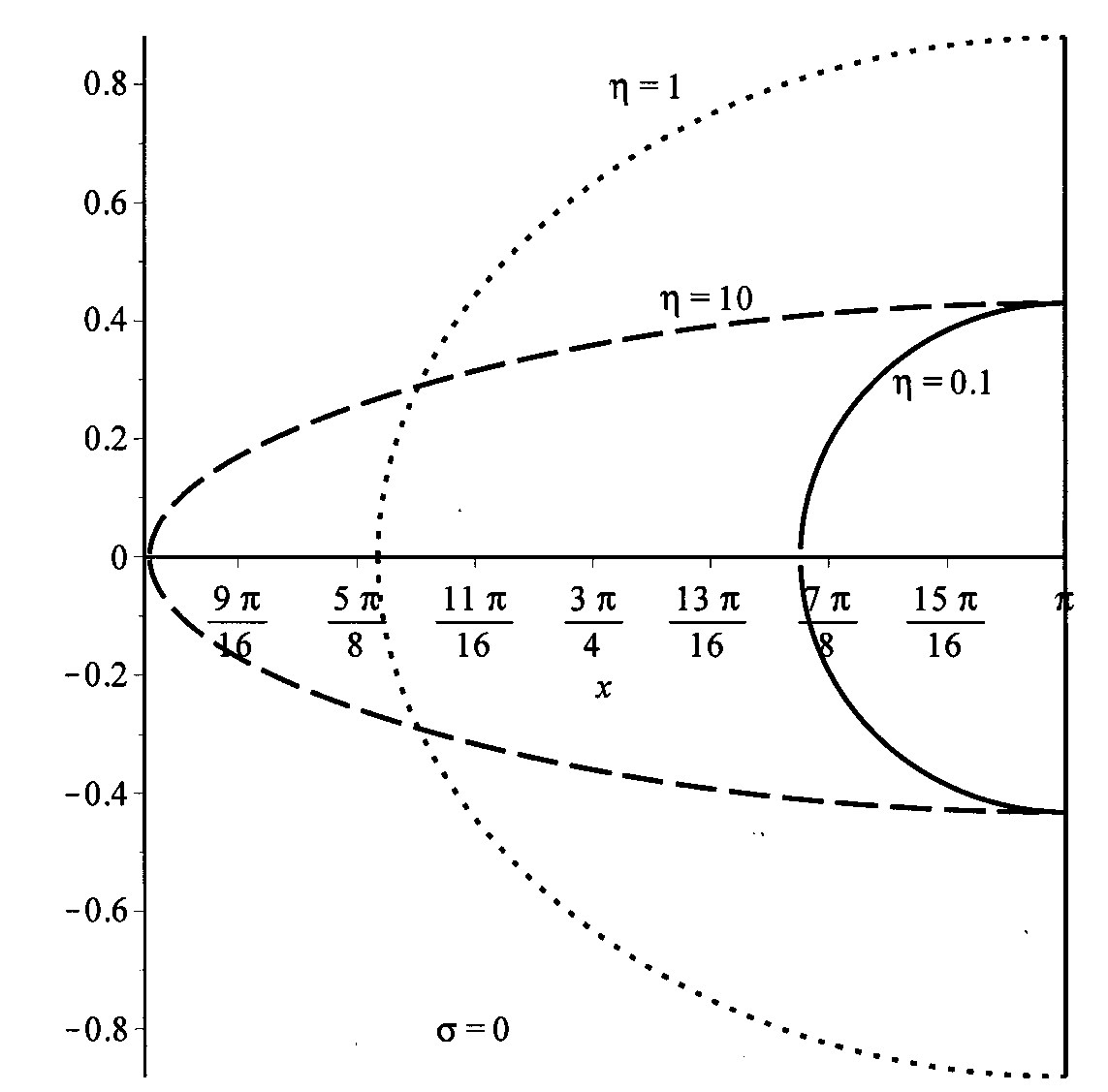
Figure 1: the special case $\sigma=0$

The empty interval $(0,x_{*})$ is not represented. The values of $x_{*}$ are respectively

$$x_{*}(\eta=0.1)=2.7\quad\quad\quad\quad x_{*}(\eta=1)=2\quad\quad\quad\quad x_{*}(\eta=10)=1.6.$$

For $x=x_{*}$ the tangent is vertical since $P_{x}=0$ while for $x=\pi-$ it is horizontal since $P_{x}\to+\infty$.

There remains the last case:

Proposition 5

For $\eta>0$ and $\sigma=-\cosh\theta\leq-1$ we have:

$$\begin{array}[]{llll}(a)&\eta\in(0,e^{-\theta})&\quad\cosh y=\left\{\begin{array}[]{ll}\displaystyle\frac{\cos x-\eta}{\sqrt{\eta^{2}+2\,\sigma\,\eta+1}}&\quad x\in\,(0,x_{-})\\[11.38109pt] \displaystyle\frac{\eta-\cos x}{\sqrt{\eta^{2}+2\sigma\,\eta+1}}&\quad x\in\,(x_{+},\pi)\end{array}\right.\\[34.1433pt] (b)&\eta\in(e^{-\theta},+\infty)&\displaystyle e^{\epsilon y_{\epsilon}}=\frac{\eta-\cos x+\sqrt{2\eta(|\sigma|-\cos x)-\sin^{2}x}}{\eta-1+\sqrt{2\eta(|\sigma|-1)}}\ \ x\in\,(0,\pi),&\\[22.76219pt] \displaystyle(c)&\eta=e^{-\theta}=\cos x_{*}&\quad\hskip 19.91692pte^{\epsilon y_{\epsilon}}=\left\{\begin{array}[]{ll}\displaystyle\frac{\cos x-\cos x_{*}}{1-\cos x_{*}}&\quad\quad x\in\,(0,x_{*})\\[11.38109pt] \displaystyle\frac{\cos x_{*}-\cos x}{\cos x_{*}+1}&\quad\quad x\in\,(x_{*},\pi)\end{array}\right.\end{array}$$ (18)

where $\epsilon=\pm 1$ and $x_{\pm}$ are defined by

$$\cos x_{\pm}=\eta\mp\sqrt{\eta^{2}+2\sigma\,\eta+1}.$$ (19)

Proof: From its derivative we see that $P_{x}^{2}$ decreases monotonically from $+\infty$ for $x\to 0+$ to $p_{*}^{2}=L^{2}\,e^{\theta}(\eta-e^{-\theta})$ for $x=x_{*}$, with $\cos x_{*}=e^{-\theta}$, and then it increases monotonically to $+\infty$ for $x\to\pi-$.

If $\eta\in(0,e^{-\theta})$ then the geodesic is defined for $x\in\,(0,x_{-})\cup(x_{+},\pi)$ with $x_{-}<x_{*}<x_{+}$ where $x_{\pm}$ are defined by (19).

So if $x\in(0,x_{-})$ we take for initial conditions $(x=x_{-},\,y=0)$ which imply $S_{+}=S_{-}=L^{2}(\cos x_{-}-\eta)$ and upon use of (11) we get the first equation of (18)(a).

If $x\in(x_{+},\pi)$ we take for initial conditions $(x=x_{+},\,y=0)$ which imply $S_{+}=S_{-}=L^{2}(\cos x_{+}-\eta)$ and upon use of (11) we get the second equation of (18)(a).

The case $\eta=e^{-\theta}$ is quite special. In this case let us define $\cos x_{*}=e^{-\theta}$. The first integral gives

$$S_{+}=2L^{2}\,e^{y}\,(\cos x-\cos x_{*})\quad\quad\quad x\in(0,x_{*})$$

and vanishes for $x\in\,(x_{*},\pi)$. Taking for initial conditions $(x=0+,y=0)$ we get the first equation of (18)(b).

The second integral is

$$S_{-}=2L^{2}\,e^{-y}\,(\cos x-\cos x_{*})\quad\quad\quad x\in(x_{*},\pi)$$

and vanishes for $x\in\,(x_{*},\pi)$. Taking for initial conditions $(x=\pi-,y=0)$ we get the second equation of (18)(b).

The remaining case $\eta\in(e^{-\theta},+\infty)$ gives a geodesic defined for $x\in\,(0,\pi)$ and in view of the structure of the quadratic integrals we can take for initial conditions $(x=0+,y=0)$. The conservation of $S_{-}/L^{2}$ gives

$$e^{-y}(\eta-\cos x+\epsilon\sqrt{2\eta(|\sigma|-\cos x)-\sin^{2}x})=\eta-1+\epsilon\sqrt{+2\eta(|\sigma|-1)}$$

and this concludes the Proof.$\quad\Box$

To conclude our analysis let us consider the case of a negative value for $\eta$ hence negative $E$. Since $P_{x}^{2}$ is invariant under the transformation $(E,\sigma,\xi)\to(-E,-\sigma,-\xi)$ it follows that $(-|E|,\sigma,\xi)$ is obtained from the above results for $(|E|,-\sigma,-\xi)$.

Let us give some examples of geodesic trajectories given by Propositions 5. For the case (a) we have

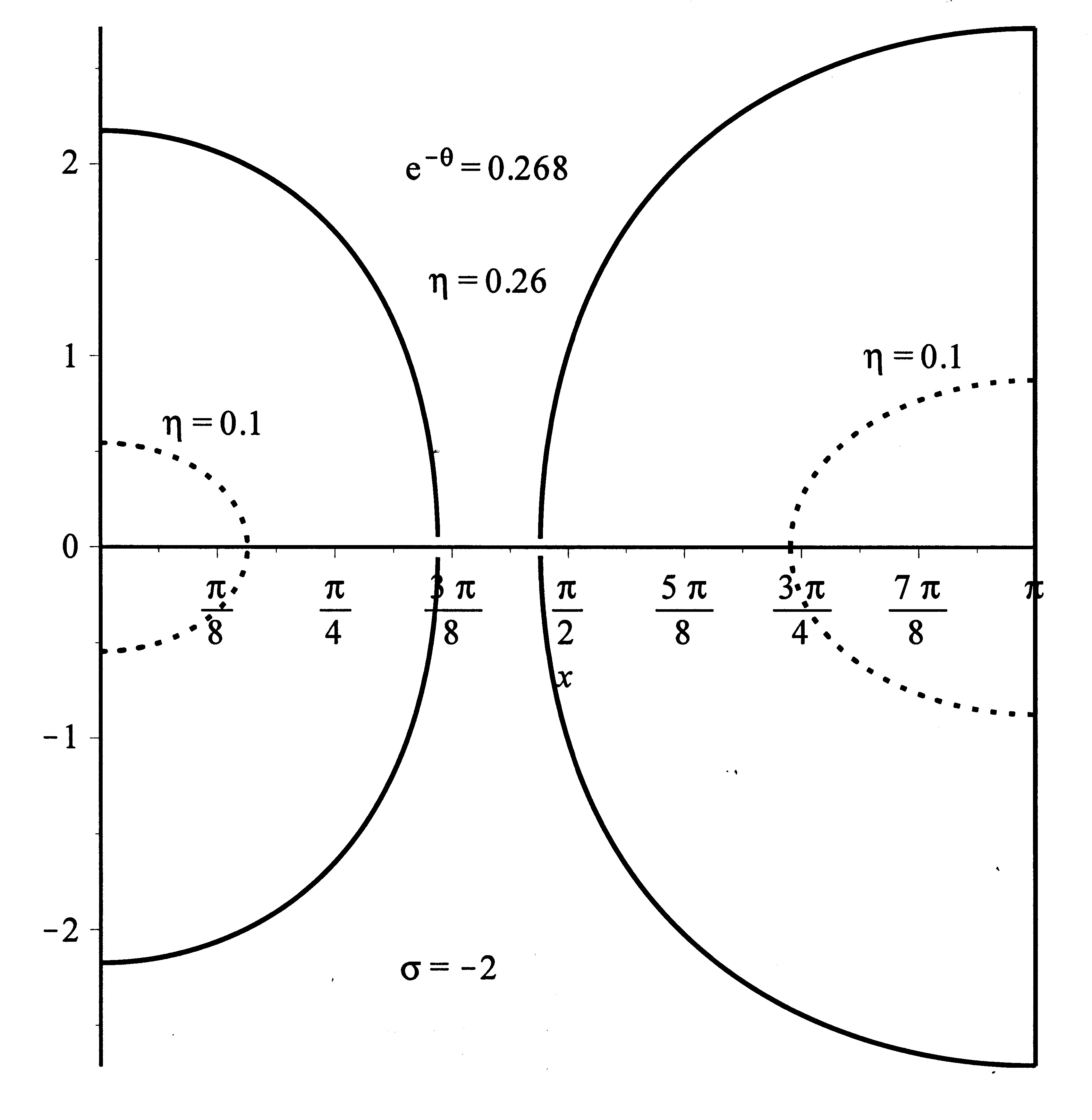
Figure 2: the case $0<\eta<e^{-\theta}$

Remarks:

• The $y$ coordinate is along the vertical.

• The hamilton equations

  $$\dot{x}=\frac{\sin^{2}x}{1-\rho\,\cos x}\,P_{x}\quad\quad\dot{y}=\frac{\sin^{2}x}{1-\rho\,\cos x}\,L\quad\quad\Longrightarrow\quad\quad\frac{dy}{dx}=\frac{L}{P_{x}}$$ (20)

  show that for $x\to 0+$ or $x\to\pi-$ the tangents to the geodesics are horizontal, while for $x=x_{-}$ or $x=x_{+}+$ they are vertical.

• The symmetry with respect to the axis $x=\pi/2$ which was apparent for vanishing energy has disappeared.

while for case (b) we have

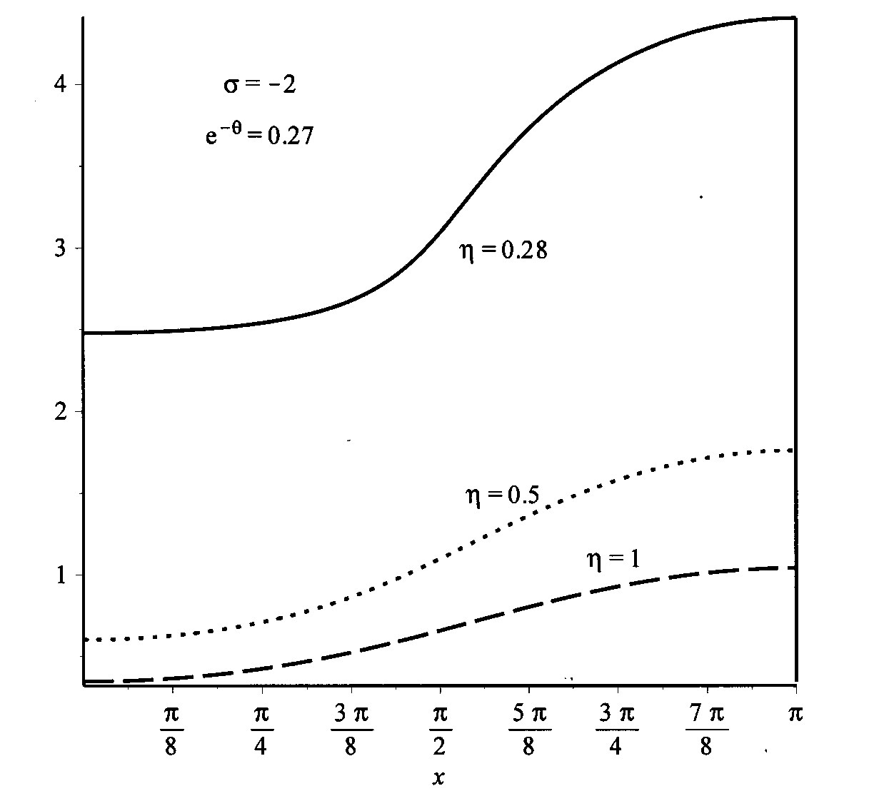
Figure 3: the case $\eta>e^{-\theta}$

In this last drawing only the geodesics with positive velocity can be seen. The negative velocity ones are obtained from $y\to-y$.

For case (c), which is quite special, we have

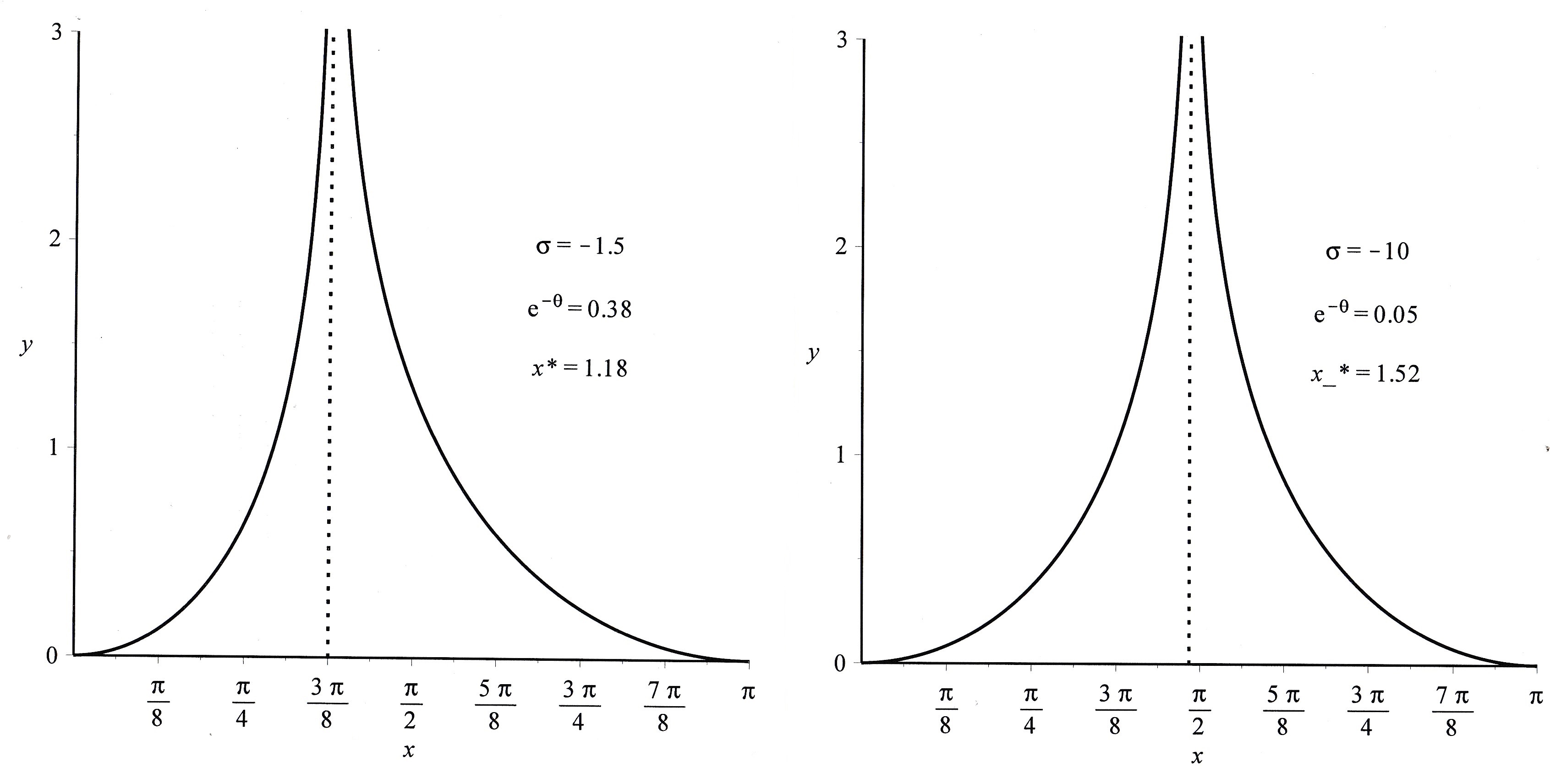
Figure 4: the case $\eta=e^{-\theta}$

The geodesics are defined only on $x\in\,(0,\pi/2)\cup(\pi/2,\pi)$ and only the positve $y$ part of the graph is shown. Since the velocity vanishes for $x=x_{*}$ the corresponding line is some kind of a wall.

For the geodesics of vanishing energy (see Proposition 3) the main difference is that for the Figures 2 and 4 the line $x=\pi/2$ becomes an axis of symmetry.

Part II THE HYPERBOLIC CASE

1 Local structure

Let us observe that for $A_{0}=0$ and $\mu=1$ the ODE   (2)(ii) leads to three different cases:

$$-A_{1}\,h\,h_{x}+A_{2}\,h_{x}=\frac{A_{3}}{2}(e^{x}+\epsilon\,e^{-x})$$ (21)

where $\ \epsilon=0,\,\pm 1.$ We have:

Proposition 6

The SI Koenigs systems

$${\cal I}_{1}=\{H,\,P_{y},\,S_{1}\}\quad\quad\quad\quad{\cal I}_{2}=\{H,\,P_{y},\,S_{2}\}$$ (22)

are given locally by three different metrics, For $\epsilon=0$ we have

$$g_{0}=(e^{-x}+\rho\,e^{-2x})(dx^{2}+dy^{2})$$ (23)

with the integrals

$$\left\{\begin{array}[]{l}S_{1}=+\cos y\,e^{x}\,P_{x}\,P_{y}+\sin y(e^{x}\,P_{y}^{2}-H)\\[11.38109pt] S_{2}=-\sin y\,e^{x}\,P_{x}\,P_{y}+\cos y(e^{x}\,P_{y}^{2}-H)\end{array}\right.$$ (24)

For $\epsilon=+1$ we have

$$g_{+}=\frac{\cosh x+\rho}{\sinh^{2}x}(dx^{2}+dy^{2})$$ (25)

with the integrals

$$\left\{\begin{array}[]{l}S_{1}=+\cos y\,\sinh x\,P_{x}\,P_{y}+\sin y(\cosh x\,P_{y}^{2}-H)\\[11.38109pt] S_{2}=-\sin y\,\sinh x\,P_{x}\,P_{y}+\cos y(\cosh x\,P_{y}^{2}-H)\end{array}\right.$$ (26)

For $\epsilon=-1$ we have

$$g_{-}=\frac{\sinh x+\rho}{\cosh^{2}x}(dx^{2}+dy^{2}).$$ (27)

with the integrals

$$\left\{\begin{array}[]{l}S_{1}=+\cos y\,\cosh x\,P_{x}\,P_{y}+\sin y(\sinh x\,P_{y}^{2}-H)\\[11.38109pt] S_{2}=-\sin y\,\cosh x\,P_{x}\,P_{y}+\cos y(\sinh x\,P_{y}^{2}-H).\end{array}\right.$$ (28)

Proof: The ODE (21) is easily integrated to

$$-\frac{A_{1}}{2}\,h^{2}+A_{2}\,h=\frac{A_{3}}{2}(e^{x}-\epsilon\,e^{-x})+\widetilde{A}_{4}.$$

If $A_{1}$ vanishes the metric is of constant curvature, so we can take $A_{1}=-2$ and $A_{2}=-2h_{0}$ ending up with

$$h-h_{0}=\pm\sqrt{\frac{A_{3}}{2}(e^{x}-\epsilon\,e^{-x})+A_{4}}\quad\quad\Longrightarrow\quad\quad h_{x}=\pm\frac{A_{3}}{4}\frac{e^{x}-\epsilon\,e^{-x}}{\sqrt{\frac{A_{3}}{2}(e^{x}-\epsilon\,e^{-x})+A_{4}}}.$$

So, up to an overall scaling, we get the three metrics given above and transforming the formulas of Matveev and Schevchishin [14] yields the quadratic integrals.$\quad\Box$

The metric ${\rm g}_{0}$ corresponds to Koenigs type II metric

$$\Big{(}a\,e^{-w}+b\,e^{-2w}\Big{)}\,du\,dv\quad\quad\quad\quad w=\frac{u+v}{2}$$

when subjected to the coordinates change $(u=x+iy,\,v=x-iy)$ and an overall scaling.

The metric ${\rm g}_{-}$ is still of type I when subjected to the coordinates change $(u=x+iy,\,v=-x+iy)$ up to scaling.

To recover the metric ${\rm g}_{+}$ as a type I, up to scaling, we have to change the parameter $a\to\,-ia$ and the coordinates $(u=x+i(y+\pi/2),\,v=-x+i(y-\pi/2))$.

Let us point out that the metric ${\rm g}_{0}$ was first obtained in [10] and the metric ${\rm g}_{+}$ in [8]. The ”new” metric ${\rm g}_{-}$ is a close cousin of ${\rm g}_{+}$ with the W-algebra:

$$\begin{array}[]{c}\{P_{y},S_{1}\}=S_{2}\quad\quad\{P_{y},S_{2}\}=-S_{1}\quad\quad\{S_{1},S_{2}\}=P_{y}\,(2P_{y}^{2}+2\rho\,H-\xi)\\[11.38109pt] S_{1}^{2}+S_{2}^{2}=H^{2}-P_{y}^{4}-P_{y}^{2}(2\rho\,H-\xi).\end{array}$$ (29)

In [10] and [8] it was shown that, keeping the same formulas for the quadratic integrals, the following potentials could be added:

$$g_{0}:\quad V_{0}=\frac{\xi}{2(1+\rho\,e^{-x})}\quad\quad g_{+}:\quad V_{+}=\frac{\xi}{2(\cosh x+\rho)}$$ (30)

while for $g_{-}$ one easily obtains:

$$V_{-}=\frac{\xi}{2(\sinh(x)+\rho)}.$$ (31)

Let us consider successively the three metrics obtained above including their potential.

2 Global structure

2.1 The metric $\mathbf{g}_{0}$

One has

Theorem 1

The SI Koenigs systems

$${\cal I}_{1}=\{H_{0},\,P_{y},\,S_{1}\}\quad\quad\quad\quad{\cal I}_{2}=\{H_{0},\,P_{y},\,S_{2}\}$$ (32)

are globally defined on the manifold $M\cong{\mathbb{H}}^{2}$ with the hamiltonian

$$H_{0}=\frac{1}{2(1+\rho\,r^{2})}\left(P_{r}^{2}+\frac{P_{\phi}^{2}}{r^{2}}+\xi\,r^{2}\right)$$ (33)

and

$$(r,\phi)\in\,(0,+\infty)\times{\mathbb{S}}^{1}\quad\quad\quad\quad(\rho,\,\xi)\in\,(0,+\infty)\times{\mathbb{R}}.$$ (34)

The integrals are

$$\left\{\begin{array}[]{l}\displaystyle S_{1}=+\cos(2\phi)\,P_{r}\,\frac{P_{\phi}}{r}+\sin(2\phi)\left(H_{0}-\frac{P_{\phi}^{2}}{r^{2}}\right)\\[14.22636pt] \displaystyle S_{2}=-\sin(2\phi)\,P_{r}\,\frac{P_{\phi}}{r}+\cos(2\phi)\left(H_{0}-\frac{P_{\phi}^{2}}{r^{2}}\right)\end{array}\right.$$ (35)

Proof: Starting from the metric (23) the change of coordinates

$$r=e^{-x/2}>0\quad\quad\quad\quad\frac{y}{2}=\phi\in\,{\mathbb{S}}^{1}$$

yields, up to scaling:

$${\rm g}=(1+\rho\,r^{2})(dr^{2}+r^{2}\,d\phi^{2})\quad\quad(r,\phi)\in\,(0,+\infty)\times{\mathbb{S}}^{1}.$$

For this metric to be riemannian we must take $\,\rho\in\,(0,+\infty)$ leading to a conformal factor which is $C^{\infty}([0,+\infty))$ and to a negative scalar curvature

$$R=-\frac{4\rho}{(1+\rho\,r^{2})^{3}}.$$

The integrals (24) are easily deduced.

To determine the manifold it is convenient to use cartesian coordinates

$$x_{1}=r\,\cos\phi\quad\quad\quad\quad x_{2}=r\,\sin\phi$$

which transform the metric into

$${\rm g}=\Big{(}1+\rho\,r^{2}\Big{)}\,{\rm g}_{0}({\mathbb{R}}^{2},{\rm can})\quad\quad\quad\quad g_{0}({\mathbb{R}}^{2},{\rm can})=dx_{1}^{2}+dx_{2}^{2}.$$

Since the conformal factor is $C^{\infty}([0,+\infty))$ we conclude that the manifold is diffeomorphic to ${\mathbb{R}}^{2}$.

Let us define

$$P_{1}=\cos\phi\,P_{r}-\frac{\sin\phi}{r}\,P_{\phi}\quad\quad P_{2}=\sin\phi\,P_{r}+\frac{\cos\phi}{r}\,P_{\phi}\quad\quad L_{3}=x_{1}\,P_{2}-x_{2}\,P_{1}$$

which generate the $e(3)$ Lie algebra with

$$\{P_{1},P_{2}\}=0\quad\quad\quad\quad\{L_{3},P_{1}\}=-P_{2}\quad\quad\quad\quad\{L_{3},P_{2}\}=P_{1}.$$

In terms of these globally defined quantities in ${\mathbb{R}}^{2}$ we have

$$H=\frac{1}{2(1+\rho(x_{1}^{2}+x_{2}^{2}))}\Big{(}P_{1}^{2}+P_{2}^{2}+\xi(x_{1}^{2}+x_{2}^{2})\Big{)}$$ (36)

and for the integrals

$$\left(\begin{array}[]{c}S_{1}\\[11.38109pt] 2S_{2}\end{array}\right)=\left(\begin{array}[]{c}P_{1}\,P_{2}\\[11.38109pt] P_{1}^{2}-P_{2}^{2}\end{array}\right)+\frac{(-\rho(P_{1}^{2}+P_{2}^{2})+\xi)}{(1+\rho(x_{1}^{2}+x_{2}^{2}))}\left(\begin{array}[]{c}x_{1}\,x_{2}\\[11.38109pt] x_{1}^{2}-x_{2}^{2}\end{array}\right)$$

concluding the proof.$\quad\Box$

2.2 The metric $\mathbf{g}_{+}$

Theorem 2

The SI Koenigs systems

$${\cal I}_{1}=\{H,\,P_{\phi},\,S_{1}\}\quad\quad\quad\quad{\cal I}_{2}=\{H,\,P_{\phi},\,S_{2}\}$$

are globally defined on the manifold $M\cong{\mathbb{H}}^{2}$. The hamiltonian is

$$H=\frac{1}{2(1+\rho\,\sinh^{2}\chi)}\left(\cosh^{2}\chi\,P_{\chi}^{2}+\frac{P_{\phi}^{2}}{\tanh^{2}\chi}+\xi\,\sinh^{2}\chi\right)$$ (37)

with

$$(\chi,\,\phi)\in\,(0,+\infty)\times{\mathbb{S}}^{1}\quad\quad\quad\quad\rho\in\,(0,1)\cup(1,+\infty)\quad\quad\quad\quad\xi\in\,{\mathbb{R}}$$

and the integrals

$$\left\{\begin{array}[]{l}\displaystyle S_{1}=+\cos(2\phi)\,P_{\chi}\,\frac{P_{\phi}}{\tanh\chi}+\sin(2\phi)\left(H-\frac{(2-\tanh^{2}\chi)}{\tanh^{2}\chi}P_{\phi}^{2}\right)\\[11.38109pt] \displaystyle S_{2}=-\sin(2\phi)\,P_{\chi}\,\frac{P_{\phi}}{\tanh\chi}+\cos(2\phi)\left(H-\frac{(2-\tanh^{2}\chi)}{\tanh^{2}\chi}P_{\phi}^{2}\right).\end{array}\right.$$ (38)

Proof: In the metric (25) we can take $x>0$ since the metric is even and we will change $\rho$ into $\widetilde{\rho}$. The scalar curvature is

$$R=-\widetilde{\rho}-\frac{(1-\widetilde{\rho}^{2})}{(\cosh x+\widetilde{\rho})^{3}}(3\cosh^{2}x+3\widetilde{\rho}\cosh x+\widetilde{\rho}^{2}-1)$$

forbids $\widetilde{\rho}=1$ which would be of constant curvature. To get a riemannian metric we must therefore restrict $\widetilde{\rho}\in\,(-1,+\infty)\backslash\{1\}$.

The change of coordinates

$$\chi=\ln\frac{1+\sqrt{u}}{1-\sqrt{u}}\in\,(0,+\infty)\quad\quad\quad\quad\frac{y}{2}=\phi\in\,{\mathbb{S}}^{1}$$

brings the metric (25) to its final form

$$g=\frac{1+\rho\,\sinh^{2}\chi}{\cosh^{2}\chi}(d\chi^{2}+\sinh^{2}\chi\,d\phi^{2})\quad\quad\quad\quad\rho=\frac{1+\widetilde{\rho}}{2}\in\,(0,+\infty)\backslash\{1\}$$

The integrals in (38) are obtained by transforming the formulas (24).

To study the global structure we need the canonical embedding of ${\mathbb{H}}^{2}\subset{\mathbb{R}}^{3}$:

$$x_{1}=\sinh\chi\,\cos\phi\quad\quad x_{2}=\sinh\chi\,\sin\phi\quad\quad x_{3}=\cosh\chi\quad\quad\chi\in\,(0,+\infty)\quad\phi\in\,{\mathbb{S}}^{1}$$

and the globally defined objects

$$M_{1}=\sin\phi\,P_{\chi}+\frac{\cos\phi}{\tanh\chi}\,P_{\phi}\quad\quad M_{2}=-\cos\phi\,P_{\chi}+\frac{\sin\phi}{\tanh\chi}\,P_{\phi}\quad\quad M_{3}=P_{\phi}$$

which generate the $sl(2,{\mathbb{R}})$ Lie algebra

$$\{M_{1},M_{2}\}=M_{3}\quad\quad\quad\quad\{M_{2},M_{3}\}=-M_{1}\quad\quad\quad\quad\{M_{3},M_{1}\}=-M_{2}.$$

One has

$$g_{0}({\rm H}^{2},{\rm can})=dx_{1}^{2}+dx_{2}^{2}-dx_{3}^{2}=d\chi^{2}+\sinh^{2}\chi\,d\phi^{2}$$

so that our metric can be written

$$g=\frac{1+\rho\,\sinh^{2}\chi}{\cosh^{2}\chi}\,g_{0}({\rm H}^{2},{\rm can})$$

and since the conformal factor is $C^{\infty}([0,+\infty))$ the manifold is diffeomorphic to ${\mathbb{H}}^{2}$.

The global definiteness on ${\mathbb{H}}^{2}$ follows from

$$H_{+}=\frac{1}{1+\rho(x_{1}^{2}+x_{2}^{2})}\Big{(}x_{3}^{2}(M_{1}^{2}+M_{2}^{2}-M_{3}^{2})+\xi(x_{1}^{2}+x_{2}^{2})\Big{)}$$

while for the integrals we have

$$\left(\begin{array}[]{c}S_{1}\\[11.38109pt] 2S_{2}\end{array}\right)=\left(\begin{array}[]{c}-M_{1}\,M_{2}\\[11.38109pt] -M_{1}^{2}+M_{2}^{2}\end{array}\right)+\frac{(1-\rho)[M_{1}^{2}+M_{2}^{2}+(x_{2}\,M_{1}-x_{1}\,M_{2})^{2}]+\xi\,x_{3}^{2}}{x_{3}^{2}[1+\rho(x_{1}^{2}+x_{2}^{2})]}\left(\begin{array}[]{c}x_{1}\,x_{2}\\[11.38109pt] x_{1}^{2}-x_{2}^{2}\end{array}\right)$$

concluding the proof. $\quad\Box$

Let us conclude with the following remark: there is a singular limit relating $H_{+}$ and $H_{0}$ which is the following:

$$\chi=\mu\,r\quad\quad P_{\chi}=\frac{P_{r}}{\mu}\quad\quad\rho=\frac{\widetilde{\rho}}{\mu^{2}}\quad\quad\xi=\frac{\widetilde{\xi}}{\mu^{4}}\quad\quad\quad\quad\mu\to 0+$$ (39)

and we have

$$\lim_{\mu\to 0+}\ \mu^{2}\,H_{+}(\chi,P_{\chi},\rho,\mu)=H_{0}(r,P_{r},\widetilde{\rho},\widetilde{\xi}\,).$$ (40)

However, due to its singular nature, it is not useful for any proof.

Let us analyze the last case:

2.3 The metric $\mathbf{g}_{-}$

We have:

Proposition 7

The metric

$${\rm g}_{-}=\frac{\sinh x+\rho}{\cosh^{2}x}(dx^{2}+dy^{2})$$ (41)

is never defined on a manifold.

Proof: Here we must take $x\in\,{\mathbb{R}}$. The metric, to be riemannian, requires $\sinh x+\rho>0$, but since the scalar curvature is

$$R=-\rho+\frac{(1+\rho^{2})}{(\sinh x+\rho)^{3}}(3\sinh^{2}x+3\rho\sinh x+\rho^{2}+1)$$

the end point $\sinh x+\rho=0$ will be a curvature singularity precluding any manifold.

This can be understood in a different way using the coordinates change

$$y=\phi\in\,{\mathbb{S}}^{1}\quad\quad x=\ln\tan\left(\frac{\theta}{2}\right):\quad\quad x\in\,{\mathbb{R}}\,\to\,\theta\in\,(0,\pi)$$

which transforms the metric into

$${\rm g}_{-}=\left(\rho-\frac{1}{\tan\theta}\right)(d\theta^{2}+\sin^{2}\theta\,d\phi^{2})=\left(\rho-\frac{1}{\tan\theta}\right)\,{\rm g}_{0}(S^{2},{\rm can}).$$

We indeed get a metric conformal to the 2-sphere, but the conformal factor is singular at the geometrical poles $\theta=0$ and $\theta=\pi$. $\quad\Box$

Let us determine the geodesic curves for the two complete metrics ${\rm g}_{0}$ and ${\rm g}_{+}$.

3 Geodesics

3.1 The geodesics of $\mathbf{g}_{0}$

Working with the hamiltonian (33) we have:

Proposition 8

The geodesics are given by:

$$\begin{array}[]{lcl}(a)&E\geq\xi/2\rho&\left\{\begin{array}[]{cl}E=0&\displaystyle\frac{L}{r^{2}}=\sqrt{|\xi|}\,\cos(2\phi)\\[11.38109pt] E\neq 0&\displaystyle\frac{L^{2}}{|E|\,r^{2}}=sign(E)+e\,\cos(2\phi)\end{array}\right.\\[28.45274pt] (b)&E_{+}<E<\xi/2\rho&\displaystyle\frac{L^{2}}{E\,r^{2}}=1+e\,\cos(2\phi)\end{array}$$ (42)

with

$$e=\sqrt{\displaystyle 1+\frac{L^{2}}{E^{2}}(2\rho\,E-\xi)}\quad\quad\quad\quad E_{\pm}=L^{2}(-\rho\,\pm\sqrt{\rho^{2}+\xi/L^{2}}).$$ (43)

Obviously for case (b) the geodesics are closed.

Proof: From the hamiltonian (33) it follows that

$$P_{r}^{2}=2E+(2\rho\,E-\xi)r^{2}-\frac{L^{2}}{r^{2}}\quad\quad(P_{r}^{2})^{\prime}=\frac{2}{r^{3}}\Big{(}(2\rho\,E-\xi)r^{4}+L^{2}\Big{)}.$$ (44)

For $\ 2\rho\,E\geq\xi\$ the function $P_{r}^{2}$ is monotonically increasing from $-\infty$ to $+\infty$. It vanishes for

$$r_{*}^{2}=\frac{L^{2}}{E+\sqrt{\Delta}}\quad\quad\quad\quad\Delta=E^{2}+L^{2}(2\rho\,E-\xi).$$

Taking for initial conditions $(r=r_{*},\,\phi=0)$ gives $S_{1}=0$ and $S_{2}=-\sqrt{\Delta}$ and upon use of (11) we obtain

$$\frac{L^{2}}{r^{2}}=E+\sqrt{\Delta}\,\cos(2\phi).$$

It follows that for $E=0$ and $E\neq 0$ we have obtained the equations in (42)(a) which describe hyperbolas.

For $2\rho\,E<\xi$ we must have $E>0$ and $\xi>0$. The derivative $(P_{r}^{2})^{\prime}$ has a simple zero for $\displaystyle r_{*}^{2}=\frac{L}{\sqrt{\xi-2\rho\,E}}$. The function $P_{r}^{2}$ increases from $-\infty$ to

$$p_{*}^{2}=2(E-\sqrt{\xi-2\rho\,E})=2\frac{(E-E_{-})(E-E_{+})}{E+\sqrt{\xi-2\rho\,E}},\quad\quad\quad\quad E_{-}<0<E_{+},$$

where $\ E_{\pm}\$ are defined in (43), and then decreases to $-\infty$. The sign of $p_{*}^{2}$ is therefore essential.

If $\ E\in\,(0,E_{+}]\$ we have $p_{*}^{2}<0$ hence $P_{r}^{2}$ is always negative and there will be no geodesic. If $\ E\in\,[E_{+},\,\xi/2\rho)\$ we will have $p_{*}^{2}>0$. The function $P_{r}^{2}$ will exhibit two simple zeroes $r_{\pm}$ such that $r_{-}<r_{*}<r_{+}$ and given by

$$r_{\pm}^{2}=\frac{E(1\pm e)}{\xi-2\rho\,E}$$

Taking for initial conditions $(r=r_{-},\,\phi=0)$ and using (11) we obtain

$$\frac{L^{2}}{r^{2}}=E+\sqrt{\Delta}\,\cos(2\phi)$$

from which we deduce (42)(b). $\quad\Box$

3.2 The geodesics of $\mathbf{g}_{+}$

We have to study the positivity of

$$P_{\chi}^{2}=2E+L^{2}+\sigma\,\tanh^{2}\chi-\frac{L^{2}}{\tanh^{2}\chi}\quad\quad\chi>0\quad\quad\sigma=2(\rho-1)E-\xi,$$ (45)

while the geodesics, using (38), are obtained from

$$S_{1}\,\sin(2\phi)+S_{2}\,\cos(2\phi)=E-\frac{(1+\cosh^{2}\chi)}{2\,\sinh^{2}\chi}\,P_{\phi}^{2}.$$ (46)

Writing the energy conservation

$$\cosh^{2}\chi\,P_{\chi}^{2}+\frac{L^{2}}{\tanh^{2}\chi}=2E\,\cosh^{2}\chi+\sigma\,\sinh^{2}\chi=2E+(2\rho\,E-\xi)\sinh^{2}\chi$$ (47)

we obtain

Lemma 1

One has the following inequalities:

$$\sigma\leq 0\quad\Longrightarrow\quad E>0\quad\quad\quad\quad\quad\quad\xi-2\rho\,E\geq 0\quad\Longrightarrow\quad E>0.$$ (48)

For the discussions to come it will be convenient to use, rather than $\chi$, the variable

$$u=\tanh^{2}\chi\ \in\ (0,1)$$

leading to

$$u\,P_{\chi}^{2}\equiv F(u)=\sigma\,u^{2}+2(E+L^{2}/2)u-L^{2}\quad\quad\quad\quad F^{\prime}(u)=\sigma+\frac{L^{2}}{u^{2}}.$$ (49)

The discussion involves two cases, according to the sign of the parameter $\xi-2\rho\,E.$

Proposition 9

For $\xi-2\rho\,E\leq 0$ the geodesic equation

$$\frac{L^{2}}{\tanh^{2}\chi}=E+\frac{L^{2}}{2}+\left|E+\frac{L^{2}}{2}\right|\,e\,\cos(2\phi)\quad\quad\quad e=\sqrt{1+\frac{L^{2}\sigma}{(E+\frac{L^{2}}{2})^{2}}}$$ (50)

does not lead to a closed curve because $e>1$.

Proof: Let us first consider the case $\sigma\geq 0$. Then the function $F$ increases monotonously from $-\infty$ to $-(\xi-2\rho\,E)$. So if $\xi-2\rho\,E\geq 0$ there is no geodesic, while for $\xi-2\rho\,E<0$ the function $F$ will be positive for $u\in(u_{-},1)$ with

$$u_{-}=\frac{L^{2}}{(E+L^{2}/2)+\sqrt{\Delta}}\quad\quad\quad\quad\Delta=(E+\frac{L^{2}}{2})^{2}+L^{2}\,\sigma.$$ (51)

The initial conditions $(u=u_{-},\,\phi=0)$ give

$$S_{1}=0\quad\quad\quad\quad S_{2}=E-L^{2}\left(\frac{1}{u_{-}}-\frac{1}{2}\right)=-\sqrt{\Delta}$$

and upon use of (46) we get (50).

The next case is for $-L^{2}\leq\sigma<0$. Then $F^{\prime}$ has a simple zero for $u_{*}=L/\sqrt{|\sigma|}\geq 1$. It follows that the variations of $F$ are the same as for $\sigma\geq 0.$ Since $\sigma<0$ we know that $E+L^{2}/2>0$ which allows to write (50) as

$$\frac{L^{2}}{\tanh^{2}\chi}=\left(E+\frac{L^{2}}{2}\right)[1+e\,\cos(2\phi)].$$

The last case is for $\sigma<-L^{2}$. This time $F^{\prime}$ has a simple zero for $u_{*}=L/\sqrt{|\sigma|}<1$ so that F increases from $-\infty$ for $u\to 0+$ to $p_{*}^{2}$ for $u=u_{*}$ and then decreases to $-(\xi-2\rho\,E)\geq 0$, where $p_{*}^{2}=(L-\sqrt{|\sigma|})^{2}-\xi+2\rho\,E.$ It follows that $F$ exhibits one simple root $u_{-}$ (given by (51)) such that $0<u_{-}<u_{*}$. Imposing the initial conditions we get again (50). $\quad\Box$

Remarks:

• For $\sigma=0$ the geodesic equation does simplify into

  $$\frac{L^{2}}{\tanh^{2}\chi}=(2E+L^{2})\,\cos^{2}\phi\quad\quad\quad E>0.$$ (52)

• For $\sigma>0$ the energy may be negative, and for the special case where $E=-L^{2}/2$ the geodesic remains well defined since we have

  $$\frac{L^{2}}{\tanh^{2}\chi}=\sqrt{\sigma}\,\cos(2\phi)\quad\quad\quad\sigma=2(\rho-1)L^{2}-\xi>0.$$ (53)

The closed geodesics will appear now:

Proposition 10

If

$$E\in\,\left[E_{+},\frac{\xi}{2\rho}\right)\quad\quad\&\quad\quad\xi-\rho\,L^{2}>0$$ (54)

where

$$E_{+}=L\Big{[}\sqrt{\xi+\rho(\rho-1)L^{2}}-(\rho-1/2)L\Big{]}$$ (55)

the geodesic equation

$$\frac{L^{2}}{\tanh^{2}\chi}=\left(E+\frac{L^{2}}{2}\right)\Big{(}1+e\,\cos(2\phi)\Big{)}$$ (56)

leads to a closed curve since $e$, still given by (50), is strictly smaller than one.

Proof: The function $P_{\chi}^{2}$ for $u\to 0+$ starts from $-\infty$ and increases monotonously to $p_{*}^{2}=2E+L^{2}-2L\sqrt{-\sigma}$ for $u=u_{*}<1$ and then decreases monotonously to $-(\xi-2\rho\,E)$ for $u\to 1-$. This time let us consider the case where $\xi-2\rho\,E>0.$ If $p_{*}^{2}<0$ no geodesic is allowed, hence let us take $p_{*}^{2}\geq 0$. It follows that $P_{\chi}^{2}$ will be positive for $u\in\,(u_{-},\,u_{+})$ such that $0<u_{-}<u_{*}<u_{+}<1$ with

$$u_{-}=\frac{L^{2}}{E+\frac{L^{2}}{2}+\sqrt{\Delta}}\quad\quad\quad\quad\quad\quad u_{+}=\frac{L^{2}}{E+\frac{L^{2}}{2}-\sqrt{\Delta}}.$$

Taking for initial conditions $(u=u_{-},\,\phi=0)$ gives

$$S_{1}=0\quad\quad\quad\quad S_{2}=E-L^{2}\left(\frac{1}{u_{-}}-\frac{1}{2}\right)=-\sqrt{\Delta}$$

and we conclude using (46).

One has to discuss the initial algebraic conditions:

$$\xi-2\rho\,E>0\quad\quad\quad\quad\sigma<-L^{2}\quad\quad\quad\quad p_{*}^{2}=(E+L^{2}/2)^{2}+L^{2}\,\sigma\geq 0$$

to show that they lead to (54). The analysis involves elementary algebra and will be skipped. $\quad\Box$

Remark: Let us observe that the geodesics of this metric ${\rm g}_{+}$ were discussed in [8]. These authors write the metric

$$g=\frac{2\cosh(2x)+b}{\sinh^{2}(2x)}(dx^{2}+dy^{2})\quad\quad x>0\quad\quad 2y\in{\mathbb{S}}^{1}\quad\quad b>-2$$

which is nothing but our metric ${\rm g}_{+}$ given by (25). In order to describe the geodesics they change the coordinates $(x,y)$ into $(r,\,\theta)$ given by

$$r=\frac{\sqrt{2\cosh(2x)+b}}{2\sinh(2x)}\in\,(0,+\infty)\quad\quad\quad\quad\theta=2y\in{\mathbb{S}}^{1}.$$

However, since we have

$$\frac{dr}{dx}=-\frac{(1+2br^{2})}{\sinh^{2}(2x)\,\sqrt{2\cosh(2x)+b}},$$

we realize that for $b\in\,(-2,0)$ this is not a local diffeomorphism hence $r$ is not a coordinate, at variance with our choice of coordinates which is valid for $b>-2$. Of course for $b>0$ we are in complete agreement with [8] albeit our coordinate $\chi$ is somewhat different from their coordinate $r$ while our $\phi$ and their $\theta$ are the same.

Part III THE AFFINE CASE

1 Local structure

The local structure, already found in [9] and [10], is given by

Proposition 11

The SI Koenigs systems

$${\cal I}_{1}=\{H,\ P_{y},\ S_{1}\}\quad\quad\quad\quad{\cal I}_{2}=\{H,\ P_{y},\ S_{2}\}$$ (57)

are given locally by

$$H=\frac{(a_{2}x+a_{1})^{2}}{a_{2}x^{2}+2a_{1}x+a_{0}}(P_{x}^{2}+P_{y}^{2})$$ (58)

with

$$\left\{\begin{array}[]{l}S_{1}=(a_{2}x+a_{1})\,P_{x}\,P_{y}-y(H-a_{2}\,P_{y}^{2})\\[11.38109pt] 2S_{2}=(a_{2}x^{2}+2a_{1}x)P_{y}^{2}+2y(a_{2}x+a_{1})\,P_{x}\,P_{y}-y^{2}(H-a_{2}\,P_{y}^{2}).\end{array}\right.$$ (59)

Proof: The ODE (2) (iii) for $A_{0}=0$ becomes

$$-A_{1}hh_{x}+A_{2}\,h_{x}=A_{3}x+A_{4}\quad\quad\Longrightarrow\quad\quad-\frac{A_{1}}{2}\,h^{2}+A_{2}\,h=\frac{A_{3}}{2}\,x^{2}+A_{4}x+A_{5}.$$

Since $A_{1}$ cannot vanish we set $A_{1}=-2$ and $A_{2}=-2h_{0}$ which leads us to

$$h=h_{0}\pm\sqrt{a_{2}x^{2}+2a_{1}x+a_{0}}\quad\quad\quad\quad h_{x}=\pm\frac{a_{2}x+a_{1}}{\sqrt{a_{2}x^{2}+2a_{1}x+a_{0}}}$$

and to the metric

$${\rm g}=P(x)\ \frac{dx^{2}+dy^{2}}{(a_{2}x+a_{1})^{2}}\quad\quad\quad\quad P(x)=a_{2}x^{2}+2a_{1}x+a_{0}$$

which implies the hamiltonian (58).$\quad\Box$

Let us compare with Koenigs results. His type III metric subjected to the coordinates change $\,(u=x+iy,\,v=-x+iy)$ gives

$${\rm g}_{K}=\left(\frac{a}{(u-v)^{2}}+b\right)\,du\,dv\quad\quad\Longrightarrow\quad\quad{\rm g}_{K}=\left(\frac{a}{4x^{2}}+b\right)(dx^{2}+dy^{2})$$ (60)

while the change of coordinate $a_{2}\,x+a_{1}\,\to\,x$, possible for $a_{2}\neq 0$, transforms our metric into:

$${\rm g}=\left(1+\frac{a_{0}-a_{1}^{2}}{x^{2}}\right)\,(dx^{2}+dy^{2}).$$ (61)

Both agree (up to an overall scaling) for $b\neq 0$ while the case $b=0$ must be excluded since one recovers a constant curvature metric.

Koenigs type IV metric, up to the same coordinates change as above gives

$${\rm g}_{K}=(u+v)\,du\,dv\quad\quad\Longrightarrow\quad\quad{\rm g}_{K}=2x(dx^{2}+dy^{2}).$$ (62)

This should be compared with our metric for $a_{2}=0$. Then we must have $a_{1}\neq 0$, otherwise the metric becomes flat, and the change of coordinate $x+a_{0}/2a_{1}\,\to\,x$ gives

$$g=x(dx^{2}+dy^{2})$$

which is Koenigs type I as pointed out in [9]. Therefore the affine case unifies at the same time Koenigs types III and IV.

2 Global structure

The scalar curvature

$$\frac{R}{2}=\frac{\Delta}{P^{3}}\Big{(}3\,(a_{2}x+a_{1})^{2}-\Delta\Big{)}\quad\quad\quad\quad\Delta=a_{1}^{2}-a_{0}\,a_{2}\neq 0$$

shows:

• That to avoid a flat metric we must impose $\Delta\neq 0$.

• That a simple zero of $P$ is a curvature singularity.

The global structure follows from

Theorem 3

The SI Koenigs systems

$${\cal I}_{1}=\{H,\ P_{y},\ S_{1}\}\quad\quad\quad\quad{\cal I}_{2}=\{H,\ P_{y},\ S_{2}\}$$ (63)

are globally defined on the manifold $M\cong{\mathbb{H}}^{2}$. The hamiltonian is

$$H=\frac{1}{2(1+\rho\,u^{2})}\Big{(}u^{2}(P_{u}^{2}+P_{y}^{2})+\xi\Big{)}\quad\quad(u,y)\in(0,+\infty)\times{\mathbb{R}}\quad\quad\rho\in(0,\infty)$$ (64)

and the integrals

$$\left\{\begin{array}[]{l}S_{1}=u\,P_{u}\,P_{y}-y(2\rho\,H-P_{y}^{2})\\[11.38109pt] 2S_{2}=-u^{2}\,P_{y}^{2}+2yu\,P_{u}\,P_{y}-y^{2}(2\rho\,H-P_{y}^{2}).\end{array}\right.$$ (65)

We have the algebraic relations

$$\{P_{y},S_{2}\}=S_{1}\quad\quad\{P_{y},S_{1}\}=P_{y}^{2}-2\rho\,H\quad\quad\{S_{1},S_{2}\}=(2S_{2}+2\,H-\xi)P_{y}$$ (66)

and

$$S_{1}^{2}+2(2\rho\,H-P_{y}^{2})S_{2}=(2\,H-\xi)P_{y}^{2}.$$ (67)

Proof: Let us organize the discussion according to the values of $a_{2}$.

If $a_{2}=0$ then $a_{1}\neq 0$ (otherwise the metric is flat) so let us take $a_{1}=1$. The coordinate $u=x+a_{0}/2$ gives the type I metric $g=u(du^{2}+dy^{2})$. This metric is riemannian iff $u>0$ and $y\in{\mathbb{R}}$. Its scalar curvature being $R=u^{-3}$ it follows that the end-point $u=0$ is a curvature singularity precluding any manifold.

If $a_{2}=1$ defining $u=x+a_{1}$ gives for the type II metric

$$g=(u^{2}-\Delta)\frac{du^{2}+dy^{2}}{u^{2}}\quad\quad\Delta=a_{1}^{2}-a_{0}\quad\quad u>0\quad\quad y\in{\mathbb{R}}.$$

Using the embedding ${\mathbb{H}}^{2}\subset{\mathbb{R}}^{3}$ given in [18]:

$$x_{1}=\frac{y}{u}\quad\quad x_{2}=\frac{1}{2u}(u^{2}+y^{2}-1)\quad\quad x_{3}=\frac{1}{2u}(u^{2}+y^{2}+1)\quad\quad u>0\quad y\in{\mathbb{R}}$$

leads to

$$g_{0}({\mathbb{H}}^{2})=dx_{1}^{2}+dx_{2}^{2}-dx_{3}^{2}=\frac{du^{2}+dy^{2}}{u^{2}}\quad\quad\Longrightarrow\quad\quad g=(u^{2}-\Delta)\,g_{0}({\mathbb{H}}^{2}).$$

So if $\Delta>0$ the conformal factor vanishes for $u=\sqrt{\Delta}$ implying a curvature singularity while if $\Delta<0$ the conformal factor never vanishes and the manifold is diffeomorphic to ${\mathbb{H}}^{2}$. Defining $\rho=-1/\Delta$, up to a scaling, we get the metric (64).

If $a_{2}=-1$ defining $u=x-a_{1}$ gives for the metric

$$g=(\Delta-u^{2})\,g_{0}({\mathbb{H}}^{2})\quad\quad\quad\quad\Delta=a_{1}^{2}+a_{0}.$$

If $\Delta>0$ the end-point $u=\sqrt{\Delta}$ will be singular, while for $\Delta<0$ we must change the overall sign to be riemannian and we are back to the case $a_{2}=1$.

The integrals are easily transformed from (59) and give (65). They allow again for a potential, which does not modify their structure. The relations (66) and (67) are then easily checked.

The global structure is best displayed using the generators defined in [18]:

$$\begin{array}[]{l}M_{1}=u\,p_{u}+y\,P_{y}\\[11.38109pt] \displaystyle M_{2}=uy\,P_{u}+\frac{(y^{2}-u^{2}-1)}{2}\,P_{y}\\[11.38109pt] \displaystyle M_{3}=uy\,P_{u}+\frac{(y^{2}-u^{2}+1)}{2}\,P_{y}\end{array}$$

which generate the $sl(2,{\mathbb{R}})$ Lie algebra. The relations

$$H=\frac{1}{2(1+\rho\,u^{2})}(M_{1}^{2}+M_{2}^{2}-M_{3}^{2}+\xi)\quad\quad\quad\quad u=\frac{x_{2}+x_{3}}{1+x_{1}^{2}}$$

and

$$S_{1}=-M_{1}(M_{2}-M_{3})-2\rho\,y\,H\quad\quad 2S_{2}=M_{2}^{2}-M_{3}^{2}-2\rho\,y^{2}\,H\quad\quad y=\frac{x_{1}(x_{2}+x_{3})}{1+x_{1}^{2}}$$

show that this system is globally defined on ${\mathbb{H}}^{2}$. $\quad\Box$

3 Geodesics

From the hamiltonian (64) we get

$$P_{u}^{2}=\frac{2E-\xi}{u^{2}}+2\rho\,E-L^{2}\quad\quad\quad\quad E\in{\mathbb{R}}\quad\quad L>0,$$ (68)

while the integrals are

$$S_{1}=L\,uP_{u}+y(L^{2}-2\rho\,E)\quad\quad\quad\quad 2S_{2}=-L^{2}\,u^{2}+2Ly\,uP_{u}+y^{2}(L^{2}-2\rho\,E).$$ (69)

We have for first case

Proposition 12

If $\ 2E<\xi\$ and $\ 2\rho\,E>L^{2}\$ the geodesic equation is

$$u^{2}-\frac{(2\rho\,E-L^{2})}{L^{2}}\,(y-y_{0})^{2}=u_{*}^{2}\quad\quad\quad\quad u\in\,(u_{*},\,+\infty)$$ (70)

where

$$u_{*}=\sqrt{\frac{\xi-2\,E}{2\rho\,E-L^{2}}}.$$

Proof: For $2E<\xi$ the classical motion is possible iff $2\rho\,E-L^{2}>0$ and for $u\in\,(u_{*},+\infty).$ Taking for initial conditions $(u=u_{*},\,\ y=y_{0})$ the conservation of $S_{1}$ gives

$$S_{1}=-y_{0}(2\rho\,E-L^{2})=L\,uP_{u}-y(2\rho\,E-L^{2})$$

which implies (70). $\quad\Box$

We have for the second case

Proposition 13

If $\ 2E=\xi\$ the geodesic degenerates into the lines

$$u=\sqrt{\frac{(2\rho\,E-L^{2})}{L^{2}}}\,|y-y_{0}|\quad\quad\quad\quad u\in\,(0,\,+\infty).$$ (71)

Proof: Using the Hamilton equations

$$\dot{u}=\pm\sqrt{(2\rho\,E-L^{2})}\frac{u^{2}}{1+\rho\,u^{2}}\quad\quad\quad\quad\dot{y}=\frac{Lu^{2}}{1+\rho\,u^{2}}$$

we get

$$\frac{du}{dy}=\pm\,\sqrt{\frac{(2\rho\,E-L^{2})}{L^{2}}}$$

which implies (71). These are the asymptotes of the hyperbolas (70). $\quad\Box$

Let us conclude with the last case:

Proposition 14

If $\ 2E>\xi\$ we have three possible types of geodesics:

$$\begin{array}[]{cll}2\rho\,E>L^{2}&\quad\quad\displaystyle u^{2}+u_{*}^{2}=\frac{(2\rho\,E-L^{2})}{L^{2}}\,(y-y_{0})^{2}&\quad\quad u\in\,(0,+\infty)\\[14.22636pt] 2\rho\,E=L^{2}&\quad\quad\displaystyle|y-y_{0}|=\frac{L}{2\sqrt{2E-\xi}}\,u^{2}&\quad\quad u\in\,(0,+\infty)\\[14.22636pt] 2\rho\,E<L^{2}&\quad\quad\displaystyle u^{2}+\frac{(2\rho\,E-L^{2})}{L^{2}}\,(y-y_{0})^{2}=u_{*}^{2}&\quad\quad u\in\,(u_{*},\,+\infty)\end{array}$$ (72)

where

$$u_{*}=\sqrt{\frac{2E-\xi}{|2\rho\,E-L^{2}|}}.$$

Proof: In the first case the positivity of $P_{u}^{2}$ allows for $u\in(0,+\infty)$. Taking for initial conditions $(u=u_{*},\,y=y_{0})$ and using as in the proof of Proposition 6 the conservation of $S_{1}$ we get the first geodesic equation.

In the second case, resorting to Hamilton equations we get

$$\frac{dy}{du}=\pm\,\frac{L}{\sqrt{2E-\xi}}\,u.$$

In the last case the positivity of $P_{u}^{2}$ requires $u\in\,(u_{*},\,+\infty)$. Taking the same initial conditions as above one gets the required result.$\quad\Box$

Remarks:

• In all the cases above we have checked that the conservation of $S_{2}$ gives the same result as the conservation of $S_{1}$.

• All the conics appear for the geodesic equations obtained here, particularly circles. This can be compared with the geodesics of the hyperbolic plane which are either circles or lines $(u>0,\,y=y_{0})$.

Part IV QUANTUM ASPECTS

1 Carter quantization

We can go a step further and examine the quantization of SI models. We will adhere to the simplest concept of “quantum superintegrability” which is the following: at the classical level we have seen that the relations

$$\{H,P_{y}\}=0\quad\quad\quad\quad\{H,S_{1}\}=0\quad\quad\quad\quad\{H,S_{2}\}=0$$ (73)

do hold. Quantizing means that to the previous classical observables we associate, by some recipee, operators $\widehat{H},\ \widehat{P}_{y},\ \widehat{S}_{1},\ \widehat{S}_{2}$ acting in the Hilbert space built up on the corresponding curved manifold.

The system will be defined as quantum superintegrable iff

$$[\widehat{H},\widehat{P}_{y}]=0\quad\quad\quad\quad[\widehat{H},\widehat{S}_{1}]=0\quad\quad\quad\quad[\widehat{H},\widehat{S}_{2}]=0.$$ (74)

While the relations (73) are rigorous, the relations (74) are most often checked only formally, which is of course required, but hides the delicacies involved in a proper definition of their self-adjoint extensions.

The simplest and most natural quantization is certainly Carter’s (or minimal) quantization (see [6]). Denoting by a hat the quantum operators and setting $\hbar=1$, the quantization rules are:

$$\widehat{Q^{i}\,P_{i}}=-\frac{i}{2}(Q^{i}\circ\nabla_{i}+\nabla_{i}\circ Q^{i})\quad\quad\widehat{S^{ij}\,P_{i}\,P_{j}}=-\nabla_{i}\circ S^{ij}\circ\nabla_{j}.$$ (75)

As a consequence we have:

Proposition 15

All of the classical SI Koenigs systems remain formally SI at the quantum level using Carter quantization.

Proof: As shown in [6] in equation (3.8), since $P_{y}$ is generated by a Killing vector, we have

$$[\widehat{H},\widehat{P_{y}}]=0.$$ (76)

For the quadratic observables, as shown in [4], if $S$ is a quadratic Killing-Stackel tensor one has

$$[\widehat{H},\widehat{S}]=\frac{2}{3}\Big{(}(\nabla_{i}\,B^{ij})\circ\nabla_{j}+\nabla_{j}\circ(\nabla_{i}B^{ij})\Big{)}$$

where

$$B^{ij}=S^{k[i}\,{\rm Ric}_{\,kl}\,g^{j]l}.$$

For a two dimensional metric which is diagonal, as it is the case for all of the Koenigs metrics, the Ricci tensor is always diagonal. It follows that the tensor $B$ vanishes identically. Therefore the classical conservation laws for $S_{1}$ and $S_{2}$ are lifted up to the quantum conservation laws

$$[\widehat{H},\widehat{S_{1}}]=0\quad\quad\quad\quad[\widehat{H},\widehat{S_{2}}]=0$$ (77)

and this concludes the proof. $\quad\Box$

Remarks:

• Let us put some emphasis on the formal character of the proof. Indeed we are working with unbounded operators defined only on dense subspaces of the Hilbert space. Computing their commutators non-formally is a very difficult task.

• One could use, as an alternative quantization, the so-called conformally equivariant quantization [5]. Then (76) is still valid while relations (77) no longer hold for this quantization.

Before diving into the hamiltonian spectrum it is of some interest to consider the action coordinates which are of conceptual interest.

2 Action coordinates for $\mathbf{g}_{0}$

We have

Proposition 16

The action coordinates, for the closed geodesics obtained in Proposition 8, are given by

$$I_{\phi}=L\quad\quad J\equiv I_{r}+I_{\phi}=\frac{E}{\sqrt{\xi-2\rho\,E}},$$ (78)

and the hamiltonian is

$$H(J)=J\Big{(}\sqrt{\xi+\rho^{2}\,J^{2}}-\rho\,J\Big{)}$$ (79)

while the quadratic integrals are

$$S_{1}=0\quad\quad\quad\quad S_{2}=-\sqrt{J^{2}-I_{\phi}^{2}}\Big{(}\sqrt{\xi+\rho^{2}\,J^{2}}-\rho\,J\Big{)}.$$ (80)

Proof: The Hamilton-Jacobi equation, starting from the action

$$S=W(r)+L\,\phi-E\,t,$$

gives trivially $I_{\phi}=L$. It remains to compute

$$I_{r}=\frac{1}{2\pi}\oint W^{\prime}\,dr=\frac{2}{\pi}\int_{r_{-}}^{r_{+}}\ W^{\prime}\,dr\quad\quad\quad\quad W^{\prime}=\sqrt{2(1+\rho\,r^{2})E-\xi\,r^{2}-\frac{L^{2}}{r^{2}}}.$$

The first change of variable

$$r\to\theta:\quad\quad\frac{L^{2}}{E\,r^{2}}=1+e\,\cos\theta\quad\quad\Longrightarrow\quad\quad I_{r}=\frac{L\,e^{2}}{\pi}\int_{0}^{\pi}\frac{\sin^{2}\theta}{(1+e\,\cos\theta)^{2}}\,d\theta,$$

and the second change $\displaystyle t=\tan\frac{\theta}{2}$ gives eventually

$$I_{r}=\frac{4Le^{2}}{\pi}\int_{-\infty}^{+\infty}\frac{t^{2}}{(1+t^{2})[1+e+(1-e)t^{2}]^{2}}\,dt$$

which is computed using the residue theorem and gives (78). As we have seen in Proposition 8 we have $\,E\in\,[E_{+},\xi/2\rho)$ where

$$E_{+}=L^{2}(-\rho\,+\sqrt{\rho^{2}+\xi/L^{2}}).$$

Differentiating

$$J=\frac{E}{\sqrt{\xi-2\rho\,E}}\quad\quad\quad\quad J=I_{r}+I_{\phi}\geq L$$

shows that $J(E)$ is a strictly increasing bijection from $E\in[E_{+},\xi/2\rho)$ to $J\in[L,+\infty)$. The inversion needed for $E(J)$ is elementary and gives (79).

The integrals follow from the initial conditions which had given $S_{1}=0$ and $S_{2}=-\sqrt{\Delta}$. Expressing $\,S_{2}$ in terms of the action variables gives (80). $\quad\Box$

Remarks:

• The hamiltonian is degenerate, a typical feature of SI systems.

• The closed geodesics stem from the potential: indeed, if $\xi=0$ there are no ellipses at all and since we have $\xi>0$ the radial component of the force derived from the potential is attractive and given by

  $$F_{r}=-\frac{\xi\,r}{(1+\rho\,r^{2})^{2}}.$$

• The knowledge of the action-angle coordinates establishes its bi-hamiltonian structure as shown by Bogoyavlenskij [3].

Let us determine, for the classical hamiltonian $H_{0}$ given by (33), the discrete spectrum of its quantum extension.

3 Point spectrum for the hamiltonian on $\mathbf{g}_{0}$

Using Carter quantization we have

$$\widehat{H_{0}}=-\frac{1}{2}\,\nabla_{i}\circ g^{ij}\circ\nabla_{j}+V(r)=-\frac{1}{2}\,\Delta+V(r)\quad\quad\quad V(r)=\frac{\xi\,r^{2}}{2(1+\rho\,r^{2})}.$$ (81)

Proposition 17

The point spectrum of $\widehat{H_{0}}$ is given by

$$E_{n,m}=\widetilde{J}\Big{(}\sqrt{\xi+\rho^{2}\,\widetilde{J}^{2}}-\rho\,\widetilde{J}\Big{)}\quad\quad\widetilde{J}=2n+|m|+1\quad\quad(n,m)\in{\mathbb{N}}\times{\mathbb{Z}},$$ (82)

and the eigenfunctions

$$\Psi_{n,m}(r,\phi)=e^{-\zeta/2}\,\zeta^{|m|/2}\,L_{n}^{|m|}(\zeta)\,e^{im\phi}\quad\quad\quad\quad\zeta=\sqrt{\xi-2\rho\,E}\ r^{2}$$ (83)

are expressed in terms of Laguerre polynomials.

Proof: We have to solve the eigenvalue problem

$$(\widehat{H_{0}}-E)\,\Psi(r,\phi)=-\frac{1}{2(1+\rho\,r^{2})}\left(\partial^{2}_{r}+\frac{1}{r}\,\partial_{r}+\frac{1}{r^{2}}\,\partial^{2}_{\phi}\right)\Psi(r,\phi)+(V(r)-E)\,\Psi(r,\phi)=0$$

for which we can take

$$\,\Psi(r,\phi)=e^{im\phi}\,\psi(r),\quad m\in{\mathbb{Z}}\quad\Longrightarrow\quad\widehat{P_{\phi}}\,\,\Psi(r,\phi)=m\,\,\Psi(r,\phi)$$

The resulting radial ODE

$$\left(\partial^{2}_{r}+\frac{1}{r}\,\partial_{r}-\frac{m^{2}}{r^{2}}+2E-(\xi-2\rho\,E)\,r^{2}\right)\psi(r)=0,$$

upon the changes

$$\zeta=\sqrt{\xi-2\rho\,E}\ r^{2}\quad\quad\quad\quad\psi(r)=e^{-\zeta/2}\zeta^{|m|/2}\,R(\zeta)$$

gives for $R$ the confluent hypergeometric ODE

$$\zeta\,R^{\prime\prime}+(c-\zeta)R^{\prime}-aR=0\quad\quad\quad\quad a=\frac{1}{2}\left(|m|+1-\frac{E}{\sqrt{\xi-2\rho\,E}}\right)\quad\quad c=|m|+1.$$

Its two independent solutions are denoted in [1] as $\Phi(a,c;\zeta)$ and $\Psi(a,c;\zeta)$ and we have to impose that the eigenfunctions are square summable i. e.

$$\int_{0}^{+\infty}\,(1+\rho\,\zeta)\,\zeta^{|m|}\,|R(\zeta)|^{2}<+\infty.$$

Taking into account the

The general solution, square integrable for $\zeta\to 0+$, is

$$\left\{\begin{array}[]{ll}m=0&\quad R(\zeta)=A_{0}\,\Phi(a_{0},1;\zeta)+B_{0}\,\Psi(a_{0},1;\zeta)\\[11.38109pt] m\neq 0&\quad R(\zeta)=A_{m}\,\Phi(a,|m|+1;\zeta)\end{array}\right.$$

For $\zeta\to+\infty$ we have

$$\Phi(a,c;\zeta)=\frac{\Gamma(c)}{\Gamma(a)}\,\zeta^{a-c}\,e^{\zeta}\left[1+{\cal O}\left(\frac{1}{\zeta}\right)\right]$$

and the exponential increase destroys the square summability. This can be avoided iff the parameter $a=-n$ with $n\in{\mathbb{N}}$ since then $\Phi$ reduces to a polynomial.

This gives

$$\widetilde{J}=\frac{E}{\sqrt{\xi-2\rho\,E}}=2n+|m|+1\quad\quad\quad\quad n\in{\mathbb{N}}\quad\quad m\in{\mathbb{Z}}.$$

Squaring produces a second degree equation for $E$ giving the expected spectrum (82).

The relations

$$\Phi(-n;|m|+1;\zeta)={n+|m|\choose n}^{-1}\,L_{n}^{|m|}(\zeta)\quad\quad\Psi(-n,1;\zeta)=(-1)^{n}\,n!\,L_{n}(\zeta)\quad\quad n\in{\mathbb{N}}$$

give (83) for the eigenfunctions. $\quad\Box$

Let us point out that the result obtained here for the energies agrees with the result obtained in [2] for $N=2$. In this reference the authors obtained the quantum energies using for separation variables the cartesian coordinates $(x_{1},\,x_{2})$. This reflects the superintegrability of this system which allows separation of variables for several different choices of coordinates.

Let us observe that in [2] the quantization is done in flat space while we have quantized in curved space. Remarkably enough both approaches lead to the same energies while, of course, the eigenfunctions are markedly different. Let us examine the relations between the two approaches.

Starting from formula (36) and quantizing in flat space the authors of [2] obtained

$$\frac{1}{2}\Big{(}\widehat{P}_{1}^{2}+\widehat{P}_{2}^{2}+\Omega^{2}(x_{1}^{2}+x_{2}^{2})\Big{)}\Psi(x_{1},x_{2})=E\,\Psi(x_{1},x_{2})\quad\quad\Omega(E)=\sqrt{\xi-2\rho\,E}$$ (84)

which is nothing but the sum of two harmonic oscillators. So the energies and eigenfunctions follow easily

$$E=(n_{1}+n_{2}+1)\Omega(E)$$ (85)

and solving this relation for $E$ we recover the formula (82) up to the identification $n_{1}+n_{2}=n+2|m|$. The eigenfunctions are expressed in terms of Hermite polynomials which become, using our polar coordinates

$${\cal H}_{n_{1},n_{2}}(\zeta,\phi)=e^{-\zeta/2}\,H_{n_{1}}(\sqrt{\zeta}\,\cos\phi)\,H_{n_{2}}(\sqrt{\zeta}\,\sin\phi).$$ (86)

The relation between these two bases of the Hilbert space, as shown in Appendix A, is given for $m\geq 0$ by

$$\begin{array}[]{l}\displaystyle 2^{2n+m}\,n!\,\Psi_{n,m}(\zeta,\phi)=\sum_{k=0}^{n}\,i^{k+m}{n\choose k}\,_{2}F_{1}\left(\begin{array}[]{c}-k,\,-m-n\\ n-k+1\end{array};-1\right)\,{\cal H}_{k,2n+m-k}(\zeta,\phi)\\[11.38109pt] \displaystyle\hskip 14.22636pt+\sum_{k=n+1}^{2n+m}\,i^{k+2n+m}{m+n\choose k-n}\,_{2}F_{1}\left(\begin{array}[]{c}k-2n-m,\,-n\\ k-n+1\end{array};-1\right)\,{\cal H}_{k,2n+m-k}(\zeta,\phi)\end{array}$$ (87)

showing that we have indeed the relation $n_{1}+n_{2}=2n+m$.

The relation $\Psi_{n,m}(\zeta,\phi)=\Psi^{*}_{n,|m|}(\zeta,\phi)$ gives the corresponding formula for $m<0$.

4 Action coordinates for $\mathbf{g}_{+}$

In proposition (10) we have seen that in some special cases the geodesics are bounded and closed. This allows us to determine the action coordinates.

Proposition 18

For the invariant torus $(H=E,\,P_{\phi}=L>0)$, with $\rho\in\,(0,1)\cup(1,+\infty)$ and $\xi>0$, we have

$$I_{\phi}=L\quad\quad I_{\chi}=-L+\sqrt{\xi-2(\rho-1)E}-\sqrt{\xi-2\rho E}\quad\quad E\in\left[E_{+},\,\frac{\xi}{2\rho}\right)$$ (88)

and the hamiltonian exhibits again degeneracy:

$$H(J)=J\left[\sqrt{\rho(\rho-1)J^{2}+\xi}-\left(\rho-\frac{1}{2}\right)J\right]\quad\quad J\equiv I_{\chi}+I_{\phi}\in\left[L,\sqrt{\frac{\xi}{\rho}}\,\right).$$ (89)

Proof: The argument is similar to the one given for the metric ${\rm g}_{0}$. We have again $I_{\phi}=L$ and it remains to compute

$$I_{\chi}=\frac{1}{2\pi}\oint P_{\chi}\,d\chi=\frac{2}{\pi}\int_{\chi_{-}}^{\chi_{+}}\ P_{\chi}\,d\chi=\frac{1}{\pi}\int_{u_{-}}^{u_{+}}\sqrt{\sigma\,u^{2}+(2E+L^{2})u-L^{2}}\,\frac{du}{u(1-u)}$$

where $u_{\pm}$, ordered as $u_{-}<u_{+}$, are the roots of the polynomial inside the square root.

The first coordinate change

$$\frac{1}{u}=r(1+e\,\cos\theta)\quad\quad r=\frac{E+L^{2}/2}{L^{2}}\quad\quad e=\sqrt{1-\frac{L^{2}|\sigma|}{(E+L^{2}/2)^{2}}}<1$$

gives

$$I_{\chi}=\frac{Lse^{2}}{\pi}\int_{0}^{\pi}\frac{\sin^{2}\theta}{(1+e\,\cos\theta)(1+se\,\cos\theta)}\,d\theta\quad\quad\quad\quad s=\frac{r}{r-1}=\frac{E+L^{2}/2}{E-L^{2}/2}>0.$$

Let us notice that

$$se-1=\frac{\sqrt{\Delta}-(E-L^{2}/2)}{E-L^{2}/2}=\frac{2L^{2}(\xi-2\rho\,E)}{(E-L^{2}/2)(\sqrt{\Delta}+(E-L^{2}/2)}<0$$

hence both $e$ and $se$ are strictly less than one.

The second coordinate change $t=\tan(\theta/2)$ gives for final result

$$I_{\chi}=\frac{4Le^{2}s}{\pi}\int_{-\infty}^{+\infty}\frac{t^{2}\,dt}{(1+t^{2})[1+e+(1-e)t^{2}][1+se+(1-se)t^{2}]}$$

which can be computed by the residue theorem and gives (88).

Differentiating this relation gives that $D_{E}\,J>0$ showing that both $J(E)$ and its inverse $E(J)$ are strictly increasing in their respective domains. The computation of $E(J)$ is easily obtained by two successive squarings. $\quad\Box$

Let us determine, for the classical hamiltonian $H_{+}$ given by (37), the discrete spectrum of its quantum extension.

5 Point spectrum for the hamiltonian on $\mathbf{g}_{+}$

Using Carter quantization we have

$$\widehat{H}_{+}=-\frac{1}{2}\,\Delta+V(\chi)\quad\quad\quad\quad V(\chi)=\frac{\xi\,\sinh^{2}\chi}{2(1+\rho\,\sinh^{2}\chi)}\quad\quad\xi>0.$$ (90)

An elegant approach was used in [2] to determine the spectrum of $\widehat{H}_{0}$. As we will see it works also for $\widehat{H}_{+}$.

5.1 Spectral analysis

The basic idea is to find coordinates for which the radial Schrödinger operator takes the form

$$-\frac{d^{2}}{dQ^{2}}+V(Q)$$ (91)

and then use some results given in [7].

The coordinate $Q$, defined as the coordinate conjugate to

$$\Pi=\frac{\cosh(\chi)}{\sqrt{1+\rho\,\sinh^{2}\chi}}\,P_{\chi},$$

is given by

$$Q(\chi)=\int_{0}^{\chi}\,\frac{\sqrt{1+\rho\,\sinh^{2}u}}{\cosh u}\,du$$ (92)

From which we deduce that the application $\chi\to Q$ is a strictly increasing $C^{\infty}$ diffeomorphism of $(0,+\infty)$ into itself with

$$Q(\chi)=\chi+{\cal O}(\chi^{3})\quad\quad\quad\quad Q(+\infty)=+\infty.$$

After the factoring $\Psi(\chi,\phi)=\psi(\chi)\,e^{im\phi}$ the ODE for $\psi(\chi)$ becomes

$$-\frac{\cosh^{2}\chi}{2(1+\rho\,\sinh^{2}\chi)}\left(\psi^{\prime\prime}+\frac{1}{\tanh\chi}\psi^{\prime}\right)+V\,\psi=E\,\psi.$$ (93)

Since we have for the norm

$$||\Psi||^{2}\propto\int_{0}^{+\infty}\,\sqrt{1+\rho\,\sinh^{2}\chi}\tanh\chi\,|\psi(\chi)|^{2}\,dQ$$

we will define

$$\psi(\chi)=(\tanh\chi)^{-1/2}(1+\rho\,\sinh^{2}\chi)^{-1/4}\,R(\chi)\quad\Rightarrow\quad||\Psi||^{2}\propto\int_{0}^{+\infty}\,|\widetilde{R}(Q)|^{2}\,dQ$$ (94)

where $\widetilde{R}=R\circ\chi$.

Transforming the ODE in (93) one obtains

$$\frac{1}{2}\left(-\frac{d^{2}\widetilde{R}}{dQ^{2}}+V_{m}(Q)\,\widetilde{R}\right)=E\,\widetilde{R}\quad\quad V_{m}=U_{m}\circ\chi$$ (95)

with the potential

$$U_{m}(\chi)=\frac{m^{2}-1/4+1/4\sinh^{2}\chi}{\tanh^{2}\chi(1+\rho\,\sinh^{2}\chi)}+2V(\chi)-\frac{(1-\rho)}{4}\frac{[2+(1-3\rho)\sinh^{2}\chi-4\rho\,\sinh^{4}\chi]}{(1+\rho\,\sinh^{2}\chi)^{3}}.$$ (96)

So we have to consider the formally symmetric operator

$$T_{m}=-\frac{d^{2}}{dQ^{2}}+V_{m}(Q){\mathbb{I}}\quad\quad\quad\quad Q\in\,(0,+\infty)\quad\quad m\in{\mathbb{Z}}$$ (97)

in the Hilbert space $L^{2}({\mathbb{R}}_{+})$. Let us prove:

Proposition 19

For all $m\in\,{\mathbb{Z}}$ there is a unique self-adjoint (s.a.) extension of $T_{m}$ having for spectrum

$$\sigma_{ess}(T_{m})=[a,+\infty)\quad\quad\quad\quad\sigma_{disc}(T_{m})\subset[0,a)$$ (98)

where

$$a=\lim_{Q\to+\infty}\,V_{m}(Q)=\frac{\widetilde{\xi}}{2\rho}\quad\quad\quad\quad\widetilde{\xi}=\xi+\frac{1}{4}\quad\quad\quad\quad\xi>0.$$ (99)

Proof: The potential is $C^{\infty}$ on ${\mathbb{R}}_{+}$ and we have for $Q\to 0+$:

$$V_{m}(Q)=\frac{m^{2}-1/4}{Q^{2}}+{\cal O}(1).$$ (100)

Let us define

$$W_{m}(Q)=V_{m}(Q)-\frac{(m^{2}-1/4)}{Q^{2}}-a\quad\quad$$ (101)

which is continuous, bounded and vanishes for $Q\to+\infty$ hence $W_{m}(Q)\,{\mathbb{I}}$ defines a compact operator on $L^{2}({\mathbb{R}}_{+})$. We may write

$$T_{m}=t_{m}+(W_{m}+a)\,{\mathbb{I}}\quad\quad\quad\quad t_{m}=-\frac{d^{2}}{dQ^{2}}+\frac{(m^{2}-1/4)}{Q^{2}}$$ (102)

where the operator $t_{m}$ is known as a Calogero hamiltonian which has been thoroughly analyzed in [7][p. 248] where the following results were proved:

• The s.a. extension of $t_{m}$ (hence for $T_{m}$) is unique for $m\neq 0$. This is not true for $m=0$, since the defect indices are $(1,1)$: there is a one parametric $U(1)$ family of self-adjoint extensions.

• The essential spectrum (simple and continuous) is:

  $$\forall m\in{\mathbb{Z}}:\quad\quad\sigma_{ess}(t_{m})=[0,+\infty).$$ (103)

Adding a compact operator does not change the essential spectrum so we have

$$\sigma_{ess}(T_{m})=\sigma_{ess}(t_{m}+a\,{\mathbb{I}}+W_{m}\,{\mathbb{I}})=\sigma_{ess}(t_{m}+a\,{\mathbb{I}})=[a,+\infty).$$ (104)

For the spectrum positivity some care is needed. For $m\neq 0$ the formal positivity implies the true positivity of its unique s.a. extension. This is no longer true for $m=0$ because we have a one parameter $U(1)$ family of s.a. extensions [7][p. 458] with the following boundary condition at $Q\to 0+$:

$$R_{\lambda}(Q)=C\Big{[}\sqrt{Q}\,\ln(k_{0}Q)\,\cos\lambda+\sqrt{Q}\sin\lambda\Big{]}+{\cal O}(Q^{3/2}\ln Q)\quad\quad\quad|\lambda|\leq\frac{\pi}{2}$$

hence for $\chi\to 0+$:

$$\psi_{\lambda}(\chi)=C\Big{[}\ln(k_{0}\chi)\,\cos\lambda+\sin\lambda\Big{]}+{\cal O}(\chi\ln\chi).$$

We will choose the Friedrichs extension (for $|\lambda|=\pi/2$) with no logarithm and positive spectrum. All the other extensions have a negative mass.

Hence we will have, for our choice of s.a. extension, that $\sigma(t_{m})\subset{\mathbb{R}}^{+}$ and the positivity of $W_{m}{\mathbb{I}}$ implies $\sigma(T_{m})\subset{\mathbb{R}}^{+}$. So we conclude that $\sigma_{disc}(T_{m})=\sigma(T_{m})\backslash\sigma_{ess}(T_{m})\subset[0,a)$ for all $m\in{\mathbb{Z}}$.$\quad\Box$

Remark: the spectral analysis developed here for $H_{+}$ would be exactly the same as for $H_{0}$ and refines the results obtained in [2]. It explains also the apparent degeneracy for $H_{0}$ of the eigenfunction with $m=0$: it is related to the non-uniqueness of the s.a. extensions.

Let us determine the explicit form of the point spectrum for $\widehat{H}_{+}$.

5.2 The point spectrum

Proposition 20

The point spectrum of $\widehat{H}_{+}$ is given by

$$E_{n,m}=\widetilde{J}\Big{[}\sqrt{\widetilde{\xi}+\rho(\rho-1)\widetilde{J}^{2}}-(\rho-1/2)\widetilde{J}\Big{]},\quad\quad\widetilde{J}=2n+|m|+1,\quad\quad\widetilde{\xi}=\xi+\frac{1}{4}.$$ (105)

where $\widetilde{J}$ is constrained by $\displaystyle\widetilde{J}<\sqrt{\widetilde{\xi}/\rho}$, hence there is a finite number of energy levels. The eigenfunctions

$$\Psi_{n,m}(\chi,\phi)=(\tanh\chi)^{|m|}\,(\cosh\chi)^{-1/2-\sqrt{\delta}}\,P_{n}^{(|m|,\sqrt{\delta})}(1-2\tanh^{2}\chi)\,e^{im\phi}\quad\delta=\widetilde{\xi}-2\rho\,E,$$ (106)

are expressed in terms of the Jacobi polynomials.

Proof: Omitting the intermediate steps already explained when dealing with $\widehat{H}_{0}$ and switching to the variable $u=\tanh^{2}\chi$, the radial ODE

$$4u^{2}(1-u)^{2}\Psi^{\prime\prime}+2u(1-u)(2-3u)\Psi^{\prime}+(\sigma\,u^{2}+2E\,u-m^{2}(1-u))\Psi=0$$

is solved by the change of function

$$\Psi(u)=u^{|m|/2}(1-u)^{1/4+\sqrt{\delta}/2}\,R(u)\quad\quad\delta=\widetilde{\xi}-2\rho\,E\quad\quad\widetilde{\xi}=\xi+\frac{1}{4}.$$

The resulting ODE for $R$ is solved by the hypergeometric function

$${}_{2}F_{1}(a_{-},a_{+};|m|+1;u)\quad\quad\quad\quad a_{\pm}=\frac{1}{2}(|m|+1+\sqrt{\delta}\pm\sqrt{\Delta})$$

where

$$\Delta=\widetilde{\xi}-2(\rho-1)E.$$

The square-summability of the wave function requires now

$$\int_{0}^{1}(1-u+\rho\,u)\frac{|R(u)^{2}|}{(1-u)^{3/2}}\,du<+\infty.$$

For $u\to 0+$ and $m\neq 0$ the second solution of the hypergeometric ODE has for behavior $R(u)\equiv u^{-|m|/2}$ which must be rejected. This is not the case for $m=0$ since then the second linearly independent solution

$${}_{2}F_{1}\left(\begin{array}[]{c}a_{-},\,a_{+}\\ 1\end{array};u\right)\,\ln u+\ldots$$

exhibits just a harmless logarithmic singularity. However , as explained in section 5.1, we consider the s.a. extension with no logarithm and this function must be rejected.

For $u\to 1-$ the key relation (see [1][vol. 1, p. 108]) is

$$\begin{array}[]{l}{}_{2}F_{1}\left(\begin{array}[]{c}a_{-},\,a_{+}\\ |m|+1\end{array};u\right)=A_{2}F_{1}\left(\begin{array}[]{c}a_{-},\,a_{+}\\ a_{-}+a_{+}-|m|\end{array};1-u\right)+\\[17.07164pt] \hskip 85.35826pt+B\,(1-u)^{|m|+1-a_{-}-a_{+}}\,_{2}F_{1}\left(\begin{array}[]{c}|m|+1-a_{-},\,|m|+1-a_{+}\\ |m|+2-a_{-}-a_{+}\end{array};1-u\right)\end{array}$$

where

$$A=\frac{\Gamma(|m|+1)\Gamma(|m|+1-a_{-}-a_{+})}{\Gamma(|m|+1-a_{-})\Gamma(|m|+1-a_{+})}\quad\quad\quad\quad B=\frac{\Gamma(|m|+1)\Gamma(a_{-}+a_{+}-|m|-1)}{\Gamma(a_{-})\Gamma(a_{+})}.$$

It shows that the first term is smooth while the second one gives for equivalent

$$R(u)\sim B\,(1-u)^{1/4-\sqrt{\delta}/2}\quad\quad\Longrightarrow\quad\quad\frac{|\Psi(u)|^{2}}{(1-u)^{3/2}}\sim B^{2}(1-u)^{-1-\sqrt{\delta}}$$

which is never integrable, except if $B=0$. This implies that we must have either $a_{+}=-n$ for $n\in{\mathbb{N}}$, which is excluded since $a_{+}$ is positive, or $a_{-}=-n$ which boils down to

$$\widetilde{J}\equiv 2n+|m|+1=\sqrt{\Delta}-\sqrt{\delta}=\sqrt{\widetilde{\xi}-2(\rho-1)E}-\sqrt{\widetilde{\xi}-2\rho E}\quad\quad\quad E\in\left(0,\frac{\widetilde{\xi}}{2\rho}\right).$$

Since the right hand side is an increasing bijection which maps

$$E\in\left(0,\frac{\widetilde{\xi}}{2\rho}\right)\ \to\ \widetilde{J}\in\left(0,\sqrt{\widetilde{\xi}/\rho}\right)\quad\quad\Longrightarrow\quad\quad\widetilde{J}<\sqrt{\widetilde{\xi}/\rho}$$

giving the required constraint. The inverse function expressing the energy in terms of $\widetilde{J}$ was already obtained in Proposition 18.

The eigenfunctions obtained can be written

$$(\tanh\chi)^{|m|}\,(\cosh\chi)^{-1/2-\sqrt{\delta}}\,_{2}F_{1}\left(\begin{array}[]{c}-n,\,n+|m|+1+\sqrt{\delta}\\ |m|+1\end{array};\tanh^{2}\chi\right)\,e^{im\phi}$$

and using the relation with Jacobi polynomials given in [1][p. 170] we obtain, up to an irrelevant factor, the relation (106). $\quad\Box$

The results obtained here are in perfect agreement with the spectral analysis developed in section (5.1).

6 Conclusion

Let us conclude with the following remarks:

• We have checked that Koenigs derivation of his SI metrics and the derivation from the framework laid down by Matveev and Shevchishin are in perfect agreement. This last approach leads, in our opinion, to a more elegant classification involving only three cases: the trigonometric, hyperbolic and affine ones.

• In the hyperbolic case, as first observed in [8], closed geodesics do appear but only for very special values of the parameters.

• The disappointing fact is that all the globally defined systems live on non-compact manifolds, namely ${\mathbb{R}}^{2}$ or ${\mathbb{H}}^{2}$. This lack of compact manifolds led Matveev and Shevchishin [14] to look for generalizations with one linear and two cubic rather than quadratic integrals. As shown in [18] one obtains cubically SI systems defined on a closed manifold, namely ${\mathbb{S}}^{2}$. In this case a direct analysis [21] proves that the metrics are Zoll i. e. all the geodesics are closed for all the values taken by the parameters.

  A more abstract proof, not relying on the detailed form of the metrics but taking into account the cubic integrals allowed Kiyohara [11] to give a different proof of the fact that the metrics must be Zoll.

  Another peculiarity of cubically SI models, at variance with Koenigs models, is that no potential is possible [13].

• Among all of the Koenigs models the one given by equation (36) in Subsection 3.1 is somewhat special. Its hamiltonian

  $$h=\frac{1}{2(1+\rho\,r^{2})}\Big{(}P_{1}^{2}+P_{2}^{2}+\xi\,r^{2}\Big{)}\quad\quad\quad\quad r^{2}=x_{1}^{2}+x_{2}^{2}$$

  was generalized quite recently by Ra$\tilde{\rm n}$ada [16] to

  $$\widetilde{H}_{a}(\kappa=-\rho,\alpha^{2}=\xi)=h+\frac{1}{(1+\rho\,r^{2})}\left(\frac{k_{1}}{x_{1}^{2}}+\frac{k_{2}}{x_{2}^{2}}\right),$$

  still quadratically SI but not globally defined since the new potential is singular at the origin.

• As shown in [19], the same hamiltonian with a different potential:

  $$\left\{\begin{array}[]{l}\displaystyle H=h+\frac{(-2\,\rho\,l\,x_{1}+m)}{2(1+\rho\,r^{2})}\\[14.22636pt] Q=2H\,L_{3}+l\,P_{2},\end{array}\right.$$ (107)

  gives a cubically integrable system.

• Changing again the potential, as shown in [20], we have

  $$\left\{\begin{array}[]{l}\displaystyle H=h+\frac{(-\rho\,k(x_{1}^{2}+x_{2}^{2})-2\,\rho\,l\,x_{1}+m)}{2(1+\rho\,r^{2})}\\[14.22636pt] Q=2H\,L_{3}^{2}+k\,L_{3}^{2}+2l\,P_{2}\,L_{3}+l^{2}\,x_{2}^{2}.\end{array}\right.$$ (108)

  which is a quartically integrable system. Quite unexpectedly the same metric, globally defined on $\,M\cong{\mathbb{R}}^{2}$, when subjected to a change of its potential, may lead either to SI or to integrable systems with integrals of various degrees in the momenta. Is this phenomenon commonplace or exceptional?

Acknowledgements: We would like to thank Philippe Briet for his kind help with the spectral analysis of Section 5.1.

Appendix A Relation between two bases

The two bases $\Psi_{n,m}$ and ${\cal H}_{n_{1},n_{2}}$ are defined in relations (83) and (86). Since they are orthogonal we must have the expansion

$$\Psi_{n,m}(\zeta,\phi)=\sum_{n_{1},n_{2}\geq 0}\,c^{n_{1},n_{2}}_{n,m}\ {\cal H}_{n_{1},n_{2}}(\zeta,\phi),$$ (A.1)

where the coefficients, using an orthogonality relation, are given by

$$2^{n_{1}+n_{2}}\,c^{n_{1},n_{2}}_{n,m}=\int_{0}^{+\infty}\,\int_{0}^{2\pi}\,\frac{{\cal H}_{n_{1},n_{2}}(\zeta,\phi)}{n_{1}!\,n_{2}!}\,\Psi_{n,m}(\zeta,\phi)\,d\zeta\,d\phi.$$ (A.2)

Using the generating function of the Hermite polynomials

$$\sum_{n\geq 0}\frac{\lambda^{n}}{n!}\,H_{n}(x)=e^{-\lambda^{2}+2\lambda\,x}$$ (A.3)

we will compute

$$S\equiv\sum_{n_{1},n_{2}\geq 0}\lambda^{n_{1}}\,\mu^{n_{2}}\,2^{n_{1}+n_{2}}\,c^{n_{1},n_{2}}_{n,m}$$ (A.4)

given by

$$S=e^{-\lambda^{2}-\mu^{2}}\int_{0}^{+\infty}\,e^{-\zeta}\zeta^{|m|/2}L_{n}^{|m|}(\zeta)\int_{0}^{2\pi}\,e^{im\phi}\,e^{2\lambda\sqrt{\zeta}\cos\phi+2\mu\sqrt{\zeta}\sin\phi}\,\frac{d\phi}{2\pi}\,d\zeta.$$ (A.5)

The $\phi$ integral, setting $z=e^{i\phi}$, becomes

$$\frac{1}{2\pi i}\oint\frac{dz}{z}\,z^{m}\,e^{(\lambda-i\mu)\sqrt{\zeta}\,z+(\lambda+i\mu)\sqrt{\zeta}/z}$$ (A.6)

where the contour is the circle of radius one. The residue theorem gives, for $m\geq 0$:

$$S=\sum_{k\geq 0}\frac{(\lambda-i\mu)^{k}}{k!}\frac{(\lambda+i\mu)^{k+m}}{(k+m)!}e^{-\lambda^{2}-\mu^{2}}\,\int_{0}^{+\infty}\,e^{-\zeta}\zeta^{k+m}L_{n}^{m}(\zeta)\,d\zeta.$$ (A.7)

This integral is computed using the Rodrigues formula for Laguerre polynomials and one obtains

$$\int_{0}^{+\infty}\,e^{-\zeta}\zeta^{k+m}L_{n}^{m}(\zeta)\,d\zeta=\left\{\begin{array}[]{ll}0&\quad\quad k\leq n-1\\[11.38109pt] \displaystyle\frac{k!}{(k-n)!}\,\frac{(m+k)!}{n!}&\quad\quad k\geq n\end{array}\right.$$ (A.8)

and the remaining sum does factorize to

$$S=\frac{(\lambda-i\mu)^{n}}{n!}\,(\lambda+i\mu)^{n+m}.$$ (A.9)

Its value for $m<0$ is merely obtained by complex conjugation.

We need to expand this function in powers of $\lambda$ and $\mu$. The binomial theorem gives

$$n!\,S=\sum_{k=0}^{m+n}\sum_{l=0}^{n}\,i^{m-k+l}{n\choose l}{m+n\choose k}\lambda^{k+l}\,\mu^{2n+m-(k+l)}$$ (A.10)

and the change of summation index $l=\nu-k$, followed by an interchange of the summations, allows to write $S=S_{1}+S_{2}$ with

$$\begin{array}[]{ll}\displaystyle n!\,S_{1}=\sum_{\nu=0}^{n}i^{\nu+m}\lambda^{\nu}\,\mu^{2n+m-\nu}\sum_{k=0}^{\nu}(-1)^{k}{m+n\choose k}{n\choose\nu-k},\\[14.22636pt] \displaystyle n!\ S_{2}=\sum_{\nu=n+1}^{2n+m}i^{\nu+m}\lambda^{\nu}\,\mu^{2n+m-\nu}\sum_{k=0}^{n}(-1)^{n-k}{m+n\choose\nu-n+k}{n\choose n-k}.\end{array}$$ (A.11)

It is convenient to use Pochammer symbols defined by

$$(a)_{0}=1\quad\quad\quad\quad(a)_{n}=a(a+1)\cdots(a+n-1)\quad n\geq 1$$

and the identities

$$(-n)_{k}=(-1)^{k}\frac{n!}{(n-k)!}\quad k\leq n\quad\quad\quad\quad(n)_{k+l}=(n)_{k}\,(n+k)_{l}$$ (A.12)

to get

$$\sum_{k=0}^{\nu}\,(-1)^{k}{m+n\choose k}{n\choose\nu-k}={n\choose\nu}\sum_{k=0}^{\nu}(-1)^{k}\frac{(-m-n)_{k}\,(-\nu)_{k}}{k!\,(n-\nu+1)_{k}}.$$ (A.13)

This last sum, expressed with Gauss hypergeometric function [1][vol. 1, p. 56], gives eventually

$$n!\,S_{1}=\sum_{\nu=0}^{n}i^{\nu+m}\,{n\choose\nu}\,_{2}F_{1}\left(\begin{array}[]{c}-\nu,-m-n\\ n-\nu+1\end{array};-1\right)\lambda^{\nu}\,\mu^{2n+m-\nu}.$$ (A.14)

The computation of $S_{2}$ is similar. The relation

$$(-1)^{n-k}{m+n\choose\nu-n+k}=(-1)^{n}{m+n\choose\nu-n}\frac{(\nu-2n-m)_{k}}{(\nu-n+1)_{k}}$$ (A.15)

gives

$$\sum_{k=0}^{n}\,(-1)^{n-k}{m+n\choose\nu-n+k}{n\choose n-l}=(-1)^{n}{m+n\choose\nu-n}\,_{2}F_{1}\left(\begin{array}[]{c}\nu-2n-m,-n\\ \nu-n+1\end{array};-1\right)$$ (A.16)

from which we conclude to

$$n!\,S_{2}=\sum_{\nu=n+1}^{2n+m}i^{\nu+2n+m}{m+n\choose\nu-n}\,_{2}F_{1}\left(\begin{array}[]{c}\nu-2n-m,-n\\ \nu-n+1\end{array};-1\right)\,\lambda^{\nu}\,\mu^{2n+m-\nu}.$$ (A.17)

Having computed $S=S_{1}+S_{2}$ and comparing the powers of $\lambda$ and $\mu$ with (A.4) ends up the proof of (87). $\quad\Box$

References

- [1] H. Bateman and A. Erdélyi, Higher Transcendental functions, volumes 1 and 2, MacGraw-Hill Book Company, New-York Toronto London (1953).
- [2] A. Ballesteros, A. Enciso, F. J. Herranz, O. Ragnisco and D. Riglioni, Ann. Phys., 326 (2011) 2053
- [3] O. I. Bogoyavlenskij, Commun. Math. Phys., 180 529
- [4] B. Carter, Phys. Rev. D,16 (1977) 3395.
- [5] C. Duval and V. Ovsienko, Sel. Math. (NS), 7 (2001) 291.
- [6] C. Duval and G. Valent, J. Math. Phys., 46 (2005) 053516.
- [7] D. M. Gitman, I. V. Tyutin and B. L. Voronov, Self-adjoint Extensions in Quantum Mechanics, Progress in Mathematical Physics 62, Birkhäuser (2012).
- [8] E. G. Kalnins, Y. Chen, Q. Li and W. Miller Jr, arXiv:1505.00527 [math-ph].
- [9] E. G. Kalnins, J. M. Kress and P. Winternitz, J. Math. Phys., 43 (2002) 970.
- [10] E. G. Kalnins, J. M. Kress, W. Miller Jr. and P. Winternitz, J. Math. Phys., 44 (2003) 5811.
- [11] S. Kiyohara, Private Communication.
- [12] G. Koenigs, note in “Leçons sur la Théorie Générale des Surfaces”, G. Darboux Vol. 4, Chelsea Publishing (1972) 368.
- [13] V. S. Matveev, Private Communication.
- [14] V. S. Matveev and V. V. Shevchishin, J. Geom. Phys., 61 (2011) 1353.
- [15] W. Miller Jr, S. Post, and P. Winternitz, J. Phys. A.: Math. Theor., 46 (2013) 423001.
- [16] M. F. Raada, J. Math. Phys., 56, 042703 (2015).
- [17] G. Thompson, J. Math. Phys., 27 (1986) 2693.
- [18] G. Valent, C. Duval and V. Shevchishin, J. Geom. Phys., 87 (2015) 461.
- [19] G. Valent, Commun. Math. Phys., 299 (2010) 631.
- [20] G. Valent, Regul. Chaotic Dyn., 18 (2013) 391.
- [21] G. Valent, Lett. Math. Phys., 104 (2014) 1121.