Statistical properties of linear-hyperbranched graft copolymers prepared via ”hypergrafting” of AB_m monomers from linear B-functional core chains: A Molecular Dynamics simulation

Abstract

The reaction of AB_m monomers ($m=2,3$) with a multifunctional B_f-type polymer chain (”hypergrafting”) is studied by coarse-grained molecular dynamics simulations. The AB_m monomers are hypergrafted using the slow monomer addition strategy. Fully dendronized, i.e., perfectly branched polymers are also simulated for comparison. The degree of branching DB of the molecules obtained with the ”hypergrafting’ process critically depends on the rate with which monomers attach to inner monomers compared to terminal monomers. This ratio is more favorable if the AB_m monomers have lower reactivity, since the free monomers then have time to diffuse inside the chain. Configurational chain properties are also determined, showing that the stretching of the polymer backbone as a consequence of the ”hypergrafting” procedure is much less pronounced than for perfectly dendronized chains. Furthermore, we analyze the scaling of various quantities with molecular weight $M$ for large $M$ ($M>100$). The Wiener index scales as $M^{2.3}$, which is intermediate between linear chains ($M^{3}$) and perfectly branched polymers ($M^{2}\ln(M)$). The polymer size, characterized by the radius of gyration $R_{g}$ or the hydrodynamic radius $R_{h}$, is found to scale as $R_{g,h}\propto M^{\nu}$ with $\nu\approx 0.38$, which lies between the exponent of diffusion limited aggregation ($\nu=0.4$) and the mean-field exponent predicted by Konkolewicz and coworkers ($\nu=0.33$).

I Introduction

Hyperbranched polymers are macromolecules with an irregular tree-like structure frey_book . Their dense structure provides them with unique mechanical and rheological properties, and the large number of functional end groups makes them interesting for applications in nanomedicine and material science gao04 ; voit09 ; irfan10 ; schuell13rev . Compared to dendrimers with a regular dendritic structure bosman99 ; grayson01 ; gillies05 ; klos09 , their synthesis is much simpler and can often be done in just one reaction step schuell13rev . One particularly promising strategy for synthesizing hyperbranched polymers is ”hypergrafting”, a ”grafting-from” approach where AB_m monomers attach to a multifunctional macroinitiator core by slow monomer addition (SMA) schuell13rev ; radke98 ; hanselmann98 ; bharathi00 ; moeck01 ; schuell12 ; schuell13 . The SMA technique allows to control the molecular weight to some extent, polydispersities are comparatively low, and it minimizes side reactions such as the formation of oligomers and cyclic side products.

Theoretical interest in hyperbranched polymers goes back to the early Fifties of the last century zimm49 ; flory52 . The polycondensation of AB_m monomers was studied by rate equations radke98 ; hanselmann98 ; schuell13 , mean-field methods lubensky79 ; isaacson80 ; stauffer82 ; cates85 ; vilgis88 ; vilgis92 ; buzza04 ; konkolewicz07 ; konkolewicz08 ; konkolewicz11 and by computer simulations of lattice konkolewicz08 ; richards07 ; wang10 ; wang11 ; juriju14 and off-lattice models lescanec90 . Simple rate equation models predict that the polydispersity index of the resulting polymers can be reduced by increasing the core functionality radke98 ; hanselmann98 ; schuell13 . Mean-field approaches have indicated that the polymers have a self-similar architecture zimm49 ; lubensky79 ; isaacson80 ; stauffer82 ; cates85 ; vilgis88 ; vilgis92 ; buzza04 . The radius of gyration was predicted to scale with the chain length according to a power law $R_{g}\sim N^{\nu}$ with Flory exponent varying between $\nu=1/4$ zimm49 and $\nu=1/2$ isaacson80 , depending on the dimensionality lubensky79 and the theoretical approach stauffer82 . In a relatively recent series of studies, Konkolewicz et al. calculated the scaling behavior of molecules created by slow monomer addition within a mean field theory that takes into account the evolution of the monomer density profile of the chains during the growth process konkolewicz07 ; konkolewicz10 ; konkolewicz08 ; konkolewicz11 . They predicted an initial logarithmic scaling for small molecules, followed by a power law scaling with exponent $\nu=1/3$ for larger molecules. They also tested their theory against experiments and simulations and found good agreement konkolewicz08 ; konkolewicz11 ; konkolewicz07b ; konkolewicz10b .

Other recent simulation studies on the generation of hyperbranched polymers were presented by Wang et al. wang10 ; wang11 and by Juriju et al. juriju14 . When comparing simulations with each other, it is important to specify the way how the hyperbranched chains were generated. In the simulations of Konkolewicz et al. konkolewicz08 , random self-avoiding walks with lengths chosen from a prescribed distribution were grown one after the other, each starting from a randomly selected branching point. In contrast, Wang et al. wang11 simulated a process of slow monomer addition under conditions of diffusion-controlled polymerization (e.g. , a polymerization via radical reactions), where the monomers diffuse into the chain from outside and attach to the first reaction site they encounter. They report Flory exponents between 1/2 and 1/3. For large molecular weights, $\nu$ is found to approach the characteristic exponent of diffusion limited aggregation (DLA), $\nu=2/5$. Juriju et al. juriju14 examined two types of growth processes and identified two distinct universality classes associated with each of them. The first is a ”quick growth” process which allows for cluster-cluster aggregation. This generates chains with a fractal structure and Flory exponent $\nu\approx 1/4$. The second is a ”slow growth” process where monomers are attached sequentially to random sites of the chain, however, without having to diffuse there first. This was found to result in dense chains where $R_{g}$ scales logarithmically with the chain length, in accordance with the theoretical prediction of Konkolewicz for short chains konkolewicz07 . Juriju et al. juriju14 also investigated the effect of excluded volume interactions and found that they have almost no influence on the results.

In the present paper, we focus on linear-hyperbranched graft copolymers (LHGCs), which have recently been proposed as an interesting alternative to standard hyperbranched polymers and dendronized polymers. Dendronized polymers have a linear backbone decorated with dendritic side chains schlueter00 ; zhang03 ; frauenrath05 , which gives them a cylindrical shape. While they are interesting macromolecular objects, their production is as cumbersome as that of dendrimers. LHGCs on the other hand also have a linear backbone, but use hyperbranched side chains instead schuell13rev ; schuell12 ; lach98 ; sun12 ; schuell12b . They can be synthesized by hypergrafting from the backbone (see Fig. 1). In a recent paper schuell13 , we have calculated the expected polydispersity index of such chains, taking into account the core dispersity, within a rate equation theory. Here we will present off-lattice Monte Carlos simulation of the growth of such chains under slow monomer addition, assuming that the polymerization reaction is diffusion controlled, and analyze the resulting topological and conformational properties.

Figure 1: Schematic example of hypergrafting of AB₂ monomers on a linear ($F_{f}$) backbone chain.

The paper is organized as follows. In the next section, we introduce the simulation model and method. Then we will discuss the properties of the resulting chains, focussing on statistical and topological properties in section III.1 and on conformational properties in section III.2. We summarize and conclude in section IV.

II Simulation Model

We use a simple bead-spring model for the chains. Beads repel each other via a repulsive WCA potential wca with diameter $\sigma$ and energy prefactor $\epsilon$, and are connected by harmonic bonds with spring constant $k=10\epsilon/\sigma^{2}$, resulting in the equilibrium distance $r_{0}\approx 1.1\sigma$. In addition, a bending potential $V_{b}=K(1-\cos(\Phi))$ is applied, where $\Phi$ is the angle between subsequent bonds and the bending constant $K$ is chosen $K=10\epsilon$. Here and throughout, the simulation units of length and energy are the interaction parameter $\sigma$ and $\epsilon$ of the WCA potential, and the time unit is $\tau=\sqrt{m\sigma/\epsilon}$, where $m$ is the mass of one bead. AB_m monomers are modelled as dimers of two beads, one bead representing the A reactive group, and the other one all the B groups. We do not include explicit solvent. Since the beads repel each other, our system corresponds to a polymer in solvent under good solvent conditions. We carry out Molecular Dynamics simulations using the Velocity-Verlet algorithm and a Langevin thermostat at temperature $k_{B}T=0.5\epsilon$ with the time step $0.005\tau$. The simulations were carried out using the open source program package ESPResSo espresso , which we extended to allow for chemical reactions between monomers and the main chain.

The monomers are created and equilibrated in a separate reservoir and then added one by one in intervals of $1000\tau$ to the main system, which initially contains one equilibrated backbone chain made of $f$ beads F. This is done by placing the monomers randomly on the surface of a sphere centered at the center of mass of the polymer, whose radius is $5\sigma$ larger than the largest distance between the center and a chain bead (A, B, or F). Fully periodic boundary conditions are applied such that monomers cannot leave the simulation box. Once they have diffused close to a chain bead, they may react with the chain, thus making the polymer grow. In that case, a new harmonic bond is established between an A bead and a B or F bead.

Reactions may take place under the following conditions

• The distance of the potential reaction partners ((A,B) or (A,F)) is less than a critical distance $r_{c}=1.1\sigma$.

• None of the beads involved in a reaction have already reached the maximum number of allowed reactions. A and F beads can react only once, B beads may react $m$ times.

• One of the partners belongs to the central chain. Reactions between free AB_m monomers are not allowed.

If these conditions are fulfilled in a given time step, the monomers react with each other with a probability $p$. We chose $p=1$ for reactions with the backbone chain ((A,F) reactions), and $p=1$ (”high reactivity”) or $p=0.01$ (”low reactivity”) for (A,B) reactions. Since monomer pairs that meet the above conditions in a given time step may still have a distance less than $r_{c}$ in the subsequent time steps, the net reactivity (i.e. , the fraction of collisions that lead to bond formation) is not equal to $p$ for $p<1$. In our simulations, we found that $p=0.01$ results in a net reactivity of roughly $r\approx 1/3$. (For $p=1$, the reactivity is obviously $r=1$.) In the present work, we take $p$ to be the same for AB${}2$ and AB₃ monomers. However, since the monomers also have to move close to each other before they can react, the resulting reaction rates may be different for AB₂ and AB₃ monomers as described below.

III Results

We will now present the simulation results, focussing first on the topological properties of the chains (i.e. , their architecture), and then on the resulting configurational properties (radius of gyration etc.).

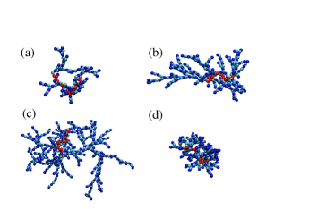
For every choice of backbone functionality $f$ ($f=20,40,100$) and monomer functionality $m$ ($m=2,3$), 20-25 independent simulation runs were carried out. For comparison, we have also simulated fully dendronized polymers with backbone functionalities $f=20,40,100$ and monomer functionalities $m=2,3$. Typical snapshots of hyperbranched polymers and one dendronized polymer are shown in Fig. 2.

Figure 2: Simulation snapshot of hyperbranched polymers with backbone length $f=20$ and monomer functionality $m=2$. The degrees of polymerization (i.e. the number of bound monomers) are (a) ${\rm DP}$=60, (b) ${\rm DP}$=140, (c) ${\rm DP}$=290. (d) shows a perfectly dendronized polymer of generation 3 on the same backbone for comparison with the hyperbranched structures (${\rm DP}$=140).

III.1 Statistical and topological properties of chains

We first address the important question how efficiently the slow monomer addition process produces highly branched molecules, i.e. , how close the resulting molecular structures are to perfectly branched, dendronized polymers. To this end, we consider

• The backbone conversion, i.e. , the average number of backbone groups that have reacted with a monomer

• the ”degree of branching” hoelter97 ; hoelter97b , which quantifies the efficiency with which the full branching capabilities of monomers are exploited in the process.

Figure 3: Mean backbone conversion as a function of the monomers per backbone unit for monomer functionality $m=2$ (top) and $m=3$ (bottom), different reactivities $r=1$ (”high”) and $r\approx 1/3$ (”low”), and different backbone functionalities $f$ as indicated. The error bars (not shown) are about twice the symbol size.

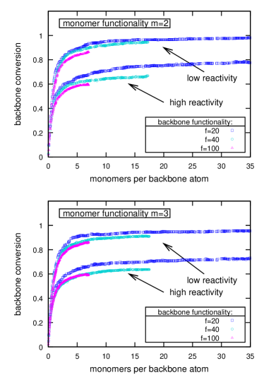
The backbone conversion is shown in Fig.  3 as a function of the grafted monomers per backbone unit in the chain - which is in some sense a time axis in the polymerization simulation. The curves for AB₂ and AB₃ monomers are very similar. In the initial regime, where monomers mainly react with backbone units, the backbone conversion increases linearly. Then, as monomers start interacting with already formed branching points, the curves deviate from linear growth and level off. For monomers with low reactivity, almost full conversion can be reached in the course of the simulation. For highly reactive monomers, a substantial fraction ($\sim 20\%$) of backbone reactive sites remain empty.

Figure 4: Mean ${\rm DB}$ as a function of monomers per backbone unit for monomer functionalities $m=2$ (top) and $m=3$ (bottom), different backbone functionalities $f$ as indicated, and different reactivities. Lines indicate theoretical predictions for different sets of rate parameters (cf. Eqs. (3-5)): $k_{r}\propto(m-r)$ (s0 and s0’); $k_{1}/k_{0}=0.45$ (s1); $k_{1}/k_{0}=0.5,k_{2}/k_{0}=0.3$ (s1’); $k_{1}/k_{0}=0.45,k_{2}/k_{0}=0.27$ (s2’), and $k_{b}=k_{0}/m$ (all sets). Sets s0,s1,s1’, and s2’ are taken from Fig. 6.

Figure 5: Mean average number of side branches ${\rm ANB}$ as a function of monomers per backbone for monomer functionalities $m=2$ (top) and $m=3$ (bottom), different backbone functionalities $f$ as indicated, and different reactivities. Lines indicate theoretical predictions for the same parameter sets as in Fig. 4.

The degree of branching can be quantified by a measure proposed by Hölter and Frey hoelter97

$${\rm DB}=\frac{m}{m-1}\>\frac{\sum_{r=1}^{m}(r-1)\>N_{r}}{\sum_{r=1}^{m}r\>N_{r}},$$ (1)

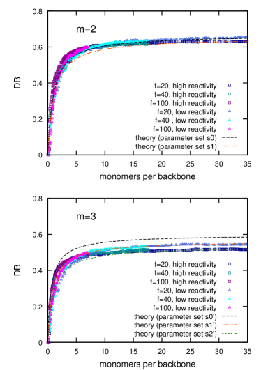
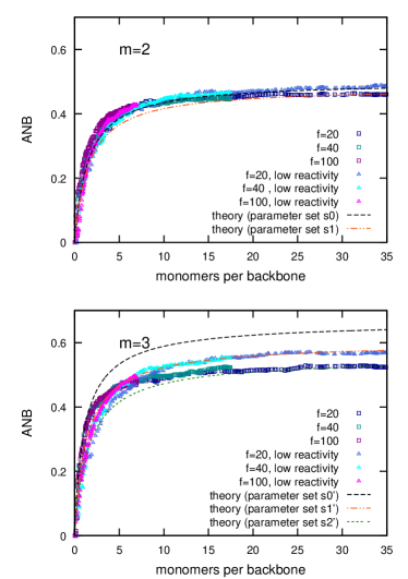
where $N_{r}$ is the number of monomers in a chain that serve as starting point for $r$ branches. (Hence $N_{0}$ is the number of terminal units, $N_{1}$ the number of linear units etc.). ${\rm DB}$ quantifies the number of side branches in the molecule relative to the total number of branches and is normalized such that it varies between 0 (linear chains) and 1 (perfectly branched dendronized chains). It is shown as a function of monomer units per backbone unit in Fig.  4. The curves look similar to those for the backbone conversion (Fig. 3): They first increase and then level off. They are higher for AB₂ monomers than for AB₃ monomers, implying that it is less likely for AB₃ than for AB₂ monomers to fill all reaction sites. Nevertheless, the total number of side branches per non-terminal monomer, quantified as

$${\rm ANB}=\frac{\sum_{r=1}^{m}(r-1)N_{r}}{\sum_{r=1}^{m}N_{r}}$$ (2)

is higher for AB₃ monomers than for AB₂ monomers as one would expect. This is shown in Fig. 5. Both DB and ANB increase slightly for less reactive monomers, but the influence of reactivity on DB and ANB is much smaller than on the backbone conversion.

The behavior of the degree of branching ${\rm DB}$ and the average number of side branches ${\rm ANB}$ can be rationalized within a simple rate equation approach proposed in Ref. hoelter97b , which we slightly modify to account for the effect of backbone conversion. The resulting equations read

$$\dot{{\color[rgb]{0,0,0}N_{F}}} = -ck_{b}{\color[rgb]{0,0,0}N_{F}}$$ (3)

$$\dot{N}_{0} = c\big{[}k_{b}{\color[rgb]{0,0,0}N_{F}}+\sum_{r=1}^{m}\>k_{r}\>N_{r}\big{]}$$ (4)

$$\dot{N}_{r} = c\big{[}k_{r-1}\>N_{r-1}-\>k_{r}\>N_{r}\big{]}:\;1\leq r\leq m$$ (5)

Here $c$ is the concentration of unreacted monomers in solution, $N_{B}$ the number of unreacted backbone sites, and $k_{r}$ gives the rate at which a free monomer reacts with a monomer that has already $r$ branches. Using these equations, one can calculate ${\rm DB}$ and ${\rm ANB}$ numerically as a function of time and derive the limiting behavior for large molecules.

In the late stages in the polymerization process, the contribution of $B$ is negligible and the relative fraction of all other units reaches a steady state, i.e. , $\dot{N}_{r}/\sum_{r}\dot{N_{r}}\propto N_{r}/\sum_{r}N_{r}$, where $\sum_{r=0}^{m}N_{r}={\rm DP}$ is the degree of polymerization. The solution becomes particularly simple if the reaction rates take the simple intuitive form $k_{r}\propto(m-r)\hat{k}$, where the combinatorial factor ($m-r$) accounts for the number of remaining available reaction sites in an AB_m monomer that has already reacted with $r$ monomers. In that case, one obtains the limiting behavior ${\rm DB}\to\frac{m}{2m-1}$ and ${\rm ANB}\to\frac{m-1}{m}$ hoelter97b . In our simulation model, we cannot expect $k_{r}\propto(m-r)\hat{k}$ to hold, since the ”reaction sites” are on the same bead. However, we can verify whether $N_{r}$ is a linear function of ${\rm DP}$ at late stages of the polymerization process as predicted, and Fig. 6 shows that this is indeed the case.

Extracting the rate constants $k_{r}$ of the theory from these data, we can then calculate ${\rm DB}$ and ${\rm ANB}$ as a function of the degree of polymerization per backbone (${\rm DP}/f$). This gives the lines shown in Figs. 4 and 5, which are in very good agreement with the simulation data except in the initial polzmerization process where molecules are still very small.

Figure 6: Average number of terminal ($N_{0}$), linear ($N_{1}$), dendritic ($N_{m}$) and semidendritic (for AB₃ monomers: $N_{2}$) units in the chains as a function of the degree of polymerization ${\rm DP}$; (a) $m=2$, high reactivity, (b) $m=2$, low reactivity, (c) $m=3$, high reactivity, (d) $m=3$, low reactivity. The backbone functionality in this example is $f=20$. The evolution of the system is compatible with the effective rate theory, Eqs. (3)–(5) (black dashed lines) with rate parameters as given in the figures and $k_{b}=k_{0}/m$ (the results are not sensitive to the choice of $k_{b}$).

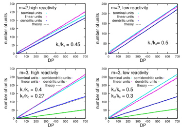
We conclude that the simulation data can be described very well by the simple rate theory. One consequence is that the degree of branching of the molecules obtained with this polymerization process mostly depends on the ratio $k_{r}/k_{0}$ of rates with which monomers attach to inner monomers compared to terminal monomers. This ratio is more favorable if monomers have lower reactivity, since the free monomers then have time to diffuse inside the chain and are not captured by the first (usually terminal) chain segments they encounter. For AB₃ monomers, the rate $k_{2}/k_{0}$ is less favorable than the rate $k_{1}/k_{0}$. This is a geometrical effect: Once a monomer has grown one side branch, it is less accessible for free monomers and the probability to grow a second side branch drops.

Apart from the degree of branching, the Wiener index $W(T)$ is another quantity that can be used to describe the topology of a branched structure with the topology of a tree $T$. It was first introduced and applied in a chemical context by Harry Wiener wiener47 , but has numerous applications in mathematics and other fields, too dobrynin01 . For a tree consisting of $N+1$ vertices (in our case monomers) connected by $N$ edges (bonds created by reactions), the Wiener index is defined as the sum over all ”distances” $s(v_{i},v_{j})$ between any two vertices $v_{i}$ and $v_{j}$,

$$W=\frac{1}{2}\sum_{ij}s(v_{i},v_{j}).$$ (6)

Here the ”distances” $s(v_{i},v_{j})$ are taken along the edges of the tree, and the length of one edge equals 1. The Wiener index and the path lengths can be used to compare densities of trees. Even though it can not be measured experimentally, it has been shown to correlate reasonably with properties such as density, viscosity and melting point bonchev92 ; widmann98 ; sheridan02 . For a linear chain consisting of $N+1$ vertices, the Wiener index is given by $W=\frac{1}{6}N(N+1)(N+2)$ and hence scales as $W\sim N^{3}$ canfield85 . It becomes smaller for branched molecules. For fully dendronized molecules, it scales as $W\sim N^{2}\ln(N)$ note ; gutman93 . $W$ can also be related to the first moment of the distribution $w(s)$ of distances or strand lengths $s$ polinska2014 . With $w(s)$ normalized as

$$w(s)=\frac{1}{N^{2}}\sum_{i,j}\delta(s-s_{ij}),$$ (7)

the Wiener index can be calculated according to $W=\frac{1}{2}N^{2}\sum s\,w(s)$. For a linear chain $w(s)$ is given by

$$w(s)=\frac{2}{s_{max}}\left(1-\frac{s}{s_{max}}\right)$$ (8)

where $s_{max}=N-1\approx N$ is the longest strand. The simulation results for these quantities are shown in Fig. 7 (Wiener index) and Fig. 8 (strand length distribution).

Figure 7: Wiener index of the hyperbranched polymers as a function of the molecular weight $M$ in units of monomer mass $M_{0}$ for monomer functionality $m=2$ (top) and $m=3$ (bottom) and different core functionalities $f$ as indicated. At high molecular weight, the Wiener index displays a power law behavior.

Figure 8: Averaged distribution of strand lengths of the hyperbranched polymers for backbone length $f=20$ (top) and $f=100$ (bottom) at different degrees of polymerization $DP$ as indicated. $DP=0$ corresponds to the bare backbone, with the distribution $w(s)$ described by Eqn. 8. The plots show the data from simulations with high reactivity. Insets show the low $s/s_{max}$ regime of the same data on a double logarithmic scale, along with a power law function (black line) to give an idea of the behavior. Here, $s_{max}$ is the average length of the longest strand.

We find that the Wiener index roughly scales as $W\sim M^{2.3}$ with the molecular weight $M=f+{\rm DP}$, hence the scaling exponent is less than that of linear chains, but higher than that expected for dendronized molecules. The monomer functionality $m$ does not have an influence on $W$, and the influence of the monomer reactivity is also very small. The distributions $w(s)$ are described by Eqn. (8) for $DP=0$ (linear initiator chains). For $DP>0$, $w(s)$ first displays an increase caused by the branched structures, followed by a decrease due to the finite length of the strands. For self similar structures, the initial increase should be described by a power law polinska2014 . Such a behavior is not clearly identified here (insets in Fig. 8). This is not surprising, given the fact that branched structures are grown on linear initiators, and that the branched structures are not much larger than the backbone, especially for long backbones $f=100$. Consistent with this, the decay of $w(s)$ after the initial increase is dominated by the linear chain behavior in this case. Interestingly, for $f=100$ at high strand lengths, the distributions increasingly deviate from the linear chain behavior with growing degree of polymerization, and a small shoulder develops at $s/s_{max}\approx 0.8$ (Fig. 8 (bottom)) . For comparison, we have also calculated the strand length distribution for ideal hyperbranched chains, which were constructed based on the rate Eqs. (3) – (5) (data not shown). The shoulder did not emerge there. We conclude that it is most likely caused by the inhomogeneous distribution of branched side chains along the backbone, which is analyzed below.

Figure 9: Normalized distribution of side chain masses for molecules with core functionality $f=100$, monomer functionality $m=2$, and total degree of polymerization ${\rm DP}=600$. One side chain hence contains 6 monomer units on average. Inset shows distribution of polymer mass along the backbone of the chains. The units of the backbone chain are labelled from 0 (one end) to 100 (other end).

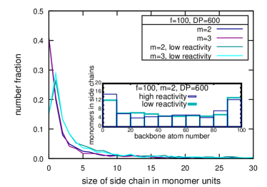
Last in this subsection, we study the distribution of monomers on the side chains. The effect of monomer reactivity on the mass distribution is illustrated in Fig. 9, which shows the histogram of masses of side chains made of AB₂ monomers in molecule with backbone functionality $f=100$ and total polymerization index ${\rm DP}=600$ . For highly reactive monomers, the curve decreases monotonically and rapidly to a value close to zero. Since the average side chain length must be 6 monomers, this implies that molecules must contain a few long side chains which compensate for the many very short chains. Decreasing the monomer reactivity reduces the fluctuations and leads to some compactification. The minimum of the distribution is shifted away from zero and the number of side chains with 1-10 monomers increases. The inset of Fig.  9 shows the mass distribution (mass in monomer units) along the backbone in the same chains. One can clearly see that the mass accumulates at both ends of the backbone. While the mass distribution is approximately uniform in the middle region, the side chains that have grown from the ends of the backbone are about twice as big on average. This effect is observed both for highly reactive monomers and for monomers with reduced reactivity. It can presumably be explained by a reduction of screening close to the backbone ends. Side branches grafted at the middle of the backbone chain are surrounded by competing side branches that may also capture monomers, hence they are less accessible for diffusing monomers than side branches grafted at the ends of the backbone.

III.2 Configurational properties

After having analyzed the topological properties of the linear-hyperbranched chains generated by the hypergrafting process, we now study the configurational properties. Specifically, we examine the the gyration radius and the hydrodynamic radius, and the amount of backbone stretching induced by hypergrafting side chains.

For ideal Gaussian chains, the radius of gyration

$$R_{g}^{2}=\frac{1}{2N^{2}}\sum_{i,j=1}^{N}(\vec{r}_{i}-\vec{r}_{j})^{2}$$ (9)

(here the sum runs over all $N$ beads of the molecules) is directly related to the Wiener index, Eq. (6), via $\langle(\vec{r}_{i}-\vec{r}_{j})^{2}\rangle\propto s(v_{i},v_{j})$. Inserting our result $W\sim N^{2.3}$, this would suggest $R_{g}\propto\sqrt{W}/N\sim N^{\nu}$ with $\nu=0.15$. However, as we shall see below, the actual exponent $\nu$ is much larger due to excluded volume effects.

Figure 10: Radius of gyration versus molecular weight (in monomer units) for monomer functionality $m=2$ (top) and $m=3$ (bottom), various backbone core functionalities $f$, and the two different choices of reactivity. Also shown for comparison are the results from simulations of linear chains. Dashed lines indicate slopes corresponding to different scaling behavior.

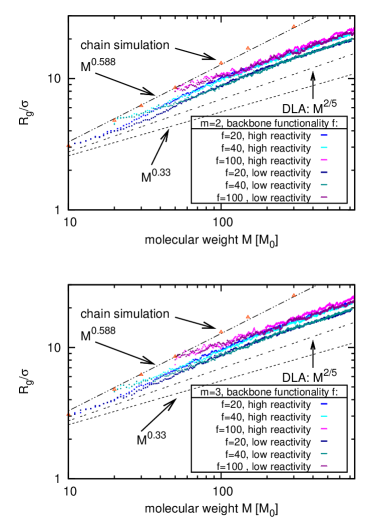
Fig. 10 summarizes our data for the radius of gyration $R_{g}$ as a function of molecular weight for all backbone functionalities $f$, monomer functionalities $m$, and the two choices of monomer reactivity. The data ware gathered ”on the fly” during the simulation of the polymerization reaction. The results for $m=2$ and $m=3$ are essentially identical. At late stages of the polymerization, all data collapse on two curves, one for high reactivity and one for low reactivity. The only exceptions are the curves for $f=100$ and low monomer reactivity, which apparently do not reach the asymptotic limit for the molecular weights under consideration. In the limit of large molecular weight, the two curves have the same slope in a double logarithmic plot. The corresponding scaling exponent, $\nu=0.38(1)$, lies between the exponent of DLA scaling ($\nu=0.4$) and the exponent predicted by Konkolewicz et al. konkolewicz07 ($\nu=0.33$), and is clearly much smaller than the Flory exponent for linear chains ($\nu=0.588$).

Figure 11: Radius of gyration versus molecular weight in monomer units for monomer functionality $m=2$ and backbone functionality $f=20$ (top) and $f=40$ (bottom). Small symbols correspond to data that were collected during the polymerization simulation, larger symbols to data that were obtained from separate, longer simulations. Also shown for comparison are data from simulations of fully dendronized polymers.

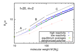
Since the data shown in Fig. 10 were gathered in a simulation of steadily growing chains, it is not clear whether they reflect the properties of fully equilibrated chains. To clarify this point, we have stored the architectures obtained for selected degrees of polymerization and studied their configurational properties by separate equilibrium simulations without monomer addition steps. The results for $R_{g}$ are shown in Fig. 11. They do not differ noticeably from the data taken in the polymerization simulation. Hence, we can conclude that the polymers in the polymerization simulation are equilibrated despite the occasional addition of one monomer. For comparison, we also show data for dendronized polymers. We find that the latter are much more compact, and in addition, the scaling of $R_{g}$ with the molecular weight seems different. Our data for the perfectly branched dendrimers are compatible with previous dendrimer simulations goetze03 ; giupponi04 that have suggested a scaling between $R_{g}\propto M^{1/5}$ (the Flory prediction) and $R_{g}\propto M^{1/3}$. The data for the hyperbranched chains suggest three different scaling regimes: An initial regime (A) with a scaling exponent of roughly $\nu\approx 0.4$, a second regime (B) where $R_{g}$ grows even stronger as a function of $M$ with an exponent $\nu\approx 0.5$, and a third regime (C) where the exponent $\nu\approx 0.4$ is recovered.

Figure 12: ”Effective exponents” (differential fractal dimensions) $\lambda={\rm d}\ln(R_{g})/{\rm d}\ln(M)$ versus molecular weight for $m=2$ (left) and $m=3$ (right). See text for explanation.

To quantify this further, we have fitted fourth order polynomials to the double logarithmic data from the polymerization runs and used them to extract local ”effective exponents”, i.e., the differential fractal dimensions $\lambda(M)={\rm d}\ln(R_{g})/{\rm d}\ln(M)$. The results, shown in Fig. 12, confirm the nonmonotonic behavior of the effective scaling. The differential fractal dimensions initially increase and then reach a peak with values that can be as large as $\lambda\sim 5.5$. The position and the height of the peak depend on the molecular details: It moves to higher values of $M$ and decreases if one increases $f$ or reduces the reactivity of the monomers. At large $M$, the differential fractal dimensions decay and reach an asymptotic value which is slightly below $\nu=0.4$. The asymptotic value is universal and does not depend noticeably on $m$, $f$, and the monomer reactivity.

Figure 13: Hydrodynamic radius versus molecular weight (in monomer units) for monomer functionality $m=2$ various backbone core functionalities $f$, and the two different choices of reactivity, compared to simulation results for linear chains. Dashed lines indicate slopes corresponding to different scaling behavior. The results for $m=3$ are basically identical.

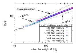
Next we discuss the hydrodynamic radius $R_{h}$, which is defined as the radius of a Stokes sphere with the same diffusion coefficient as the polymer and which we calculate via the approximate equation doi_edwards

$$\frac{1}{R_{h}}=\frac{1}{N(N-1)}\sum_{i=1}^{N}\sum_{j\neq i}\frac{1}{|\vec{r}_{i}-\vec{r}_{j}|}.$$ (10)

In the asymptotic limit, the scaling of $R_{h}$ and $R_{g}$ should be the same. In the simulations, the results for $R_{h}$ are very similar to those for $R_{g}$, therefore we only show the data from polymerization runs for $m=2$ as an example (Fig. 13). Much like in Fig. 10, the data collapse onto two curves corresponding to high and low reactivity. The two curves show a similar scaling behavior, which again differs distinctly from that of linear chains. We note that the scaling of $R_{h}$ for linear chains does not quite reach the asymptotic limit $R_{h}\propto M^{\nu}$ with $\nu=0.588$ in our system, the apparent exponent ($\nu\approx 0.53$) is slightly smaller. This is in agreement with results from other simulations and experiments reith02 . In contrast, the scaling exponent of $R_{h}$ for the largest hyperbranched chains, $\nu\approx 0.43(1)$, is slightly larger than that measured for $R_{g}$.

Figure 14: Ratio $R_{g}/R_{h}$ as a function of molecular weight in monomer units for hyperbranched chains with monomer functionality $m=2$ and backbone functionality $f=20$ (left) and $f=40$ (right). Data for linear chains and fully dendronized molecules (same backbone length) are also shown for comparison.

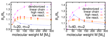
The internal structure can be further investigated by inspecting the ratio $R_{g}/R_{h}$. The value of $R_{g}/R_{h}$ depends on the molecular architecture. For long ideal chains, it is known to be 1.5; experiments with linear polymers give slightly smaller values bantle82 . Dendrimers have been reported to have ratios close to 1, star polymers with polydisperse arms have $R_{g}/R_{h}\approx 1.2$ burchard99 ; reith02b . Fig. 14 shows the data for $R_{g}/R_{h}$ from equilibrium simulations for monomer functionality $m=2$ and backbone length $f=20$ and $f=40$. Upon increasing the molecular weight, one observes a distinct peak at $M\approx 50-100$ and a subsequent slight decrease. A similar peak has been reported by Wang et al. wang11 in simulations of hyperbranched polymers with a pointlike core. In our simulations, we observe that the peak is less pronounced for longer backbone (core)chains. It almost vanishes at $f=40$ and completely disappears at $f=100$ (not shown). One can rationalize the peak as follows: Starting from a linear chain, the polymer first develops into a star shaped form with growing side chain number. With increasing size of side chains and degree of branching, the overall structure becomes more spherical, i.e. , $R_{g}/R_{h}$ decreases again. Dendronized molecules show a similar behavior with an even more pronounced peak, whereas in linear polymers, $R_{g}/R_{h}$ grows monotonously as a function of $M$.

Figure 15: Average end-to-end distance of the backbone chain as a function of the degree of polymerization (the number of hypergrafted monomers) for backbone lengths $f=20$ (top) and $f=40$ (bottom). The black symbols represent the averages from equilibrium simulations and the values from simulations of dendronized polymers.

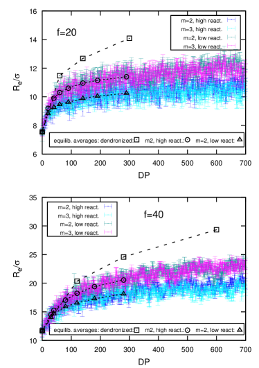
Finally, we address the question whether and how the backbone chain stretches due to the growth of side chains. Naively, one might expect that the stiffness, i.e. , the persistence length of the backbone chain, can be tuned in a controlled manner by hypergrafting branched side chains. However, extensive simulations of bottle-brush polymers have indicated that the persistence length is no longer a well-defined concept for such chains hsu10 . The same should hold for linear-hyperbranched chains. Therefore, we will not discuss the stiffness of the backbone here, but rather its elongation. The average end-to-end distance $R_{e}$ is shown in Fig. 15 as a function of the number ${\rm DP}$ of grafted monomers for backbones of length $f=20$ and $f=40$ and monomer functionality $m=2$. One can clearly distinguish two regimes: In the initial regime up to ${\rm DP}\sim f$, where monomers attach directly to the backbone, $R_{e}$ increases sharply with ${\rm DP}$. Then, the curves level off and continue to increase much more slowly, such that the additional stretching of $R_{e}$ relative to the end-to-end distance of the bare backbone is only of order $10^{-4}$ per additional grafted monomer. We expect that this curve will further flatten at much higher ${\rm DP}$ once $R_{e}$ becomes comparable to the contour length, but this regime was not reached in the simulations. If monomers have reduced reactivity, the range of the first regime is slightly extended and $R_{e}$ increases. The slope of $R_{e}$ in the second high ${\rm DP}$-regime does not seem to depend on the monomer reactivity.

For comparison, we have also studied the end-to-end distance of the corresponding dendronized molecules. The behavior in the initial regime is quantitatively similar to that of hyperbranched chains. In the second regime, the slope is much larger. This underlines once more the fundamental differences between dendronized molecules and hyperbranched molecules.

IV Discussion and Conclusion

We have studied the structural and conformational properties of linear-hyperbranched copolymers by computer simulations of a simple, solvent-free, coarse-grained spring-bead model. The model is designed to mimic the synthesis of linear-hyperbranched copolymers in good solvent under conditions of slow monomer addition. Our main results can be summarized as follows:

The topological properties of the hyperbranched chain (the chain architecture) are intermediate between those of linear and dendronized chains. The evolution of the numbers of branching points with different coordination numbers as a function total polymerization agreement is in very good agreement to a simple rate theory proposed by Hölter and Frey hoelter97b , despite the fact that the theory neglects screening and excluded volume effects. The theory predicts an upper limit for the degree of branching, hence our results suggest that the dendronized limit cannot be reached on principle. The Wiener index $W$ is found to scale with the scaling exponent $W\propto M^{\omega}$ with $\omega\approx 2.3$, which is between the exponents for dendrimers ($\omega=2$ with logarithmic corrections) and linear chains ($\omega=3$).

Likewise, the behavior of the polymer size (as specified by the radius of gyration $R_{g}$ or the hydrodynamic radius $R_{h}$) as a function of molecular weight is intermediate between that of linear and dendronized chains. The scaling exponent is found to be around $\nu\approx 0.38$, closer to the exponent of diffusion limited aggregation than to other exponents suggested in the literature (1/2, 1/3, 1/4). However, the asymptotic regime might not have been reached, and we cannot exclude the possibility that the true exponent is $\nu=1/3$ as predicted by Konkolewicz et al. konkolewicz07 . At small molecular weights, the exponent is nonmonotonic and varies between 0.4 and 0.5.

We should note that these questions are not only of academic interest. Molecular weight distributions of polymers are often measured by chromatography, and they are calibrated by comparison with linear polymers of known length. Thus one implicitly assumes that the hydrodynamic radii of the target chains and the calibration chains behave similarly as a function of molecular weight. If the exponent $\nu$ deviates significangly for both architectures, the analysis becomes questionable and correction terms must be applied. This requires a good knowledge of $\nu$ in the target chain. Unfortunately, our results suggest that neither linear chains nor fully dendronized chains are good reference systems.

We have specifically addressed the question, whether molecules can be made more compact by reducing the monomer reactivity. We find that reducing the reactivity by a factor of three has relatively little influence on the degree of branching and no influence on the scaling properties of both structural and conformational properties of the chains. It does, however, influence the prefactor in the asymptotic power law for $R_{g}$ and $R_{h}$. Hence the chains are more compact, but their behavior does not change qualitatively.

We have also studied the distribution of monomers on the side chains and found that it depends on the grafting point of the side chains on the core backbone. For long backbone chains, the side chains that have polymerized at their ends are about twice as long as the ones in the middle, leading to a pom-pom like structure. This somewhat unexpected result of the present study will also have implications for the synthesis and resulting properties of such structures.

Finally, we have examined the influence of the side chains on the conformations of the backbone chain. As one would expect, linear backbone chains stretch out if side chains are hypergrafted to them. However, the effect is much less pronounced than for dendronized chains.

Since our simulations are done with an implicit solvent model, they do not include hydrodynamic interactions. In fluids at rest, hydrodynamics should not be important on the time scales relevant for slow monomer addition. This might change if one applies flow externally, and it might be possible to manipulate the synthesis process by applying external flows, e.g. , in microfluidic setups. For example, linear-hyperbranched copolymers might stretch in flow at high Weissenberg numbers, which should facilitate the grafting of monomers to inner side chains. This will be the subject of future investigations.