On mapping theorems for numerical range

Abstract.

Let $T$ be an operator on a Hilbert space $H$ with numerical radius $w(T)\leq 1$. According to a theorem of Berger and Stampfli, if $f$ is a function in the disk algebra such that $f(0)=0$, then $w(f(T))\leq\|f\|_{\infty}$. We give a new and elementary proof of this result using finite Blaschke products.

A well-known result relating numerical radius and norm says $\|T\|\leq 2w(T)$. We obtain a local improvement of this estimate, namely, if $w(T)\leq 1$ then

$$\|Tx\|^{2}\leq 2+2\sqrt{1-|\langle Tx,x\rangle|^{2}}\qquad(x\in H,~{}\|x\|\leq 1).$$

Using this refinement, we give a simplified proof of Drury’s teardrop theorem, which extends the Berger–Stampfli theorem to the case $f(0)\neq 0$.

1. Introduction

Let $H$ be a complex Hilbert space and $T$ be a bounded linear operator on $H$. The numerical range of $T$ is defined by

$$W(T):=\{\langle Tx,x\rangle:x\in H,~{}\|x\|=1\}.$$

It is a convex set whose closure contains the spectrum of $T$. If $\dim H<\infty$, then $W(T)$ is compact. The numerical radius of $T$ is defined by

$$w(T):=\sup\{|\langle Tx,x\rangle|:x\in H,~{}\|x\|=1\}.$$

It is related to the operator norm via the double inequality

(1.1) $$\|T\|/2\leq w(T)\leq\|T\|.$$

If further $T$ is self-adjoint, then $w(T)=\|T\|$. For proofs of these facts and further background on numerical range we refer to the book of Gustafson and Rao [8].

This paper arose from an attempt to gain a better understanding of mapping theorems for numerical ranges. In contrast with spectra, it is not true in general that $W(p(T))=p(W(T))$ for polynomials $p$, nor is it true if we take convex hulls of both sides. However, some partial results do hold. Perhaps the most famous of these is the power inequality: for all $n\geq 1$, we have

$$w(T^{n})\leq w(T)^{n}.$$

This was conjectured by Halmos and, after several partial results, was established by Berger [2] using dilation theory. An elementary proof was given by Pearcy in [10]. A more general result was established by Berger and Stampfli in [3] for functions in the disk algebra (namely functions that are continuous on the closed unit disk and holomorphic on the open unit disk). They showed that, if $w(T)\leq 1$, then, for all $f$ in the disk algebra such that $f(0)=0$, we have

$$w(f(T))\leq\|f\|_{\infty}.$$

Again their proof used dilation theory. In §2 below, we give an elementary proof of this result along the lines of Pearcy’s proof of the power inequality.

The assumption that $f(0)=0$ is essential in the Berger–Stampfli theorem, as is shown by an example in [3]. Without this assumption, the situation becomes more complicated. The best result in this setting is Drury’s teardrop theorem [6], which will be discussed in detail in §4 below. At the heart of the teardrop theorem is an operator inequality, which Drury proved by citing a decomposition theorem of Dritschel and Woerdeman [5], and then performing some complicated calculations. It turns out that these difficulties can be circumvented by exploiting a refinement of the inequality (1.1). We establish this refinement in §3 and show how it can be used to simplify Drury’s argument in §4. In §5 we make some concluding remarks.

2. An elementary proof of the Berger–Stampfli mapping theorem

In this section we present an elementary proof of the aforementioned theorem of Berger and Stampfli. Here is the formal statement of the theorem.

Theorem 2.1.

Let $H$ be a complex Hilbert space, let $T$ be a bounded linear operator on $H$ with $w(T)\leq 1$, and let $f$ be a function in the disk algebra such that $f(0)=0$. Then $w(f(T))\leq\|f\|_{\infty}$.

We require two folklore lemmas about finite Blaschke products. Let us write ${\mathbb{D}}$ for the open unit disk and ${\mathbb{T}}$ for the unit circle.

Lemma 2.2.

Let $B$ be a finite Blaschke product. Then $\zeta B^{\prime}(\zeta)/B(\zeta)$ is real and strictly positive for all $\zeta\in{\mathbb{T}}$.

Proof.

We can write

$$B(z)=c\prod_{k=1}^{n}\frac{a_{k}-z}{1-\overline{a}_{k}z},$$

where $a_{1},\dots,a_{n}\in{\mathbb{D}}$ and $c\in{\mathbb{T}}$. Then

$$\frac{B^{\prime}(z)}{B(z)}=\sum_{k=1}^{n}\frac{1-|a_{k}|^{2}}{(z-a_{k})(1-\overline{a}_{k}z)}.$$

In particular, if $\zeta\in{\mathbb{T}}$, then

$$\frac{\zeta B^{\prime}(\zeta)}{B(\zeta)}=\sum_{k=1}^{n}\frac{1-|a_{k}|^{2}}{|\zeta-a_{k}|^{2}},$$

which is real and strictly positive. ∎

Lemma 2.3.

Let $B$ be a Blaschke product of degree $n$ such that $B(0)=0$. Then, given $\gamma\in{\mathbb{T}}$, there exist $\zeta_{1},\dots,\zeta_{n}\in{\mathbb{T}}$ and $c_{1},\dots,c_{n}>0$ such that

(2.1) $$\frac{1}{1-\overline{\gamma}B(z)}=\sum_{k=1}^{n}\frac{c_{k}}{1-\overline{\zeta}_{k}z}.$$

Proof.

Given $\gamma\in{\mathbb{T}}$, the roots of the equation $B(z)=\gamma$ lie on the unit circle, and by Lemma 2.2 they are simple. Call them $\zeta_{1},\dots,\zeta_{n}$. Then $1/(1-\overline{\gamma}B)$ has simple poles at the $\zeta_{k}$. Also, as $B(0)=0$, we have $B(\infty)=\infty$ and so $1/(1-\overline{\gamma}B)$ vanishes at $\infty$. Expanding it in partial fractions gives (2.1), for some choice of $c_{1},\dots,c_{n}\in{\mathbb{C}}$.

The coefficients $c_{k}$ are easily evaluated. Indeed, from (2.1) we have

$$c_{k}=\lim_{z\to\zeta_{k}}\frac{1-\overline{\zeta}_{k}z}{1-\overline{\gamma}B(z)}=\lim_{z\to\zeta_{k}}\frac{(\zeta_{k}-z)/\zeta_{k}}{(B(\zeta_{k})-B(z))/B(\zeta_{k})}=\frac{B(\zeta_{k})}{\zeta_{k}B^{\prime}(\zeta_{k})}.$$

In particular $c_{k}>0$ by Lemma 2.2. ∎

Proof of Theorem 2.1.

Suppose first that $f$ is a finite Blaschke product $B$. Suppose also that the spectrum $\sigma(T)$ of $T$ lies within the open unit disk ${\mathbb{D}}$. By the spectral mapping theorem $\sigma(B(T))=B(\sigma(T))\subset{\mathbb{D}}$ as well. Let $x\in H$ with $\|x\|=1$. Given $\gamma\in{\mathbb{T}}$, let $\zeta_{1},\dots,\zeta_{n}\in{\mathbb{T}}$ and $c_{1},\dots,c_{n}>0$ as in Lemma 2.3. Then we have

$$1-\overline{\gamma}\langle B(T)x,x\rangle =\langle(I-\overline{\gamma}B(T))x,x\rangle$$

$$=\langle y,(I-\overline{\gamma}B(T))^{-1}y\rangle \text{where~{}}y:=(I-\overline{\gamma}B(T))x$$

$$=\Bigl{\langle}y,\sum_{k=1}^{n}c_{k}(I-\overline{\zeta}_{k}T)^{-1}y\Bigr{\rangle} \text{by~{}}\eqref{E:Blaschke2}$$

$$=\sum_{k=1}^{n}c_{k}\langle(I-\overline{\zeta}_{k}T)z_{k},z_{k}\rangle \text{where~{}}z_{k}:=(I-\overline{\zeta}_{k}T)^{-1}y$$

$$=\sum_{k=1}^{n}c_{k}(\|z_{k}\|^{2}-\overline{\zeta}_{k}\langle Tz_{k},z_{k}\rangle).$$

Since $w(T)\leq 1$, we have $\operatorname{Re}(\|z_{k}\|^{2}-\overline{\zeta}_{k}\langle Tz_{k},z_{k}\rangle)\geq 0$, and as $c_{k}>0$ for all $k$, it follows that

$$\operatorname{Re}(1-\overline{\gamma}\langle B(T)x,x\rangle)\geq 0.$$

As this holds for all $\gamma\in{\mathbb{T}}$ and all $x$ of norm $1$, it follows that $w(B(T))\leq 1$.

Next we relax the assumption on $f$, still assuming that $\sigma(T)\subset{\mathbb{D}}$. We can suppose that $\|f\|_{\infty}=1$. Then there exists a sequence of finite Blaschke products $B_{n}$ that converges locally uniformly to $f$ in ${\mathbb{D}}$. (This is Carathéodory’s theorem: a simple proof can be found in [7, §1.2].) Moreover, as $f(0)=0$, we can also arrange that $B_{n}(0)=0$ for all $n$. By what we have proved, $w(B_{n}(T))\leq 1$ for all $n$. Also $B_{n}(T)$ converges in norm to $f(T)$, because $\sigma(T)\subset{\mathbb{D}}$. It follows that $w(f(T))\leq 1$, as required.

Finally we relax the assumption that $\sigma(T)\subset{\mathbb{D}}$. By what we have already proved, $w(f(rT))\leq\|f\|_{\infty}$ for all $r<1$. Interpreting $f(T)$ as $\lim_{r\to 1^{-}}f(rT)$, it follows that $w(f(T))\leq\|f\|_{\infty}$, provided that this limit exists. In particular this is true when $f$ is holomorphic in a neighborhood of $\overline{{\mathbb{D}}}$. To prove the existence of the limit in the general case, we proceed as follows. Given $r,s\in(0,1)$, the function $g_{rs}(z):=f(rz)-f(sz)$ is holomorphic in a neighborhood of $\overline{{\mathbb{D}}}$ and vanishes at $0$, so, by what we have already proved, $w(g_{rs}(T))\leq\|g_{rs}\|_{\infty}$. Therefore,

$$\|f(rT)-f(sT)\|=\|g_{rs}(T)\|\leq 2w(g_{rs}(T))\leq 2\|g_{rs}\|_{\infty}.$$

The right-hand side tends to zero as $r,s\to 1^{-}$, so, by the usual Cauchy-sequence argument, $f(rT)$ converges as $r\to 1^{-}$. This completes the proof. ∎

3. A local inequality relating norm to numerical radius

Let $T$ be a bounded operator on a Hilbert space $H$ and let $x\in H$. The left-hand inequality in (1.1) amounts to saying that $\|Tx\|\leq 2$ whenever $w(T)\leq 1$ and $\|x\|\leq 1$. In this section we establish the following local refinement.

Theorem 3.1.

If $w(T)\leq 1$ and $\|x\|\leq 1$, then

(3.1) $$\|Tx\|^{2}\leq 2+2\sqrt{1-|\langle Tx,x\rangle|^{2}}.$$

Proof.

We may as well suppose that $\|x\|=1$. Multiplying $T$ by a unimodular scalar, we may further suppose that $\langle Tx,x\rangle\geq 0$. Set $A:=(T+T^{*})/2$ and $B:=(T-T^{*})/2i$. By the triangle inequality, we then have

$$\|Tx-\langle Tx,x\rangle x\|\leq\|Ax-\langle Ax,x\rangle x\|+\|Bx-\langle Bx,x\rangle x\|.$$

Now, by Pythagoras’ theorem,

$$\|Tx-\langle Tx,x\rangle x\|^{2}=\|Tx\|^{2}-|\langle Tx,x\rangle|^{2},$$

and likewise for $A$ and $B$. Also $A$ and $B$ are self-adjoint operators and have numerical radius at most $1$, so $\|A\|\leq 1$ and $\|B\|\leq 1$. Further, the condition $\langle Tx,x\rangle\geq 0$ implies that $\langle Ax,x\rangle=\langle Tx,x\rangle$ and $\langle Bx,x\rangle=0$. Hence

$$\|Ax-\langle Ax,x\rangle x\|^{2} =\|Ax\|^{2}-|\langle Ax,x\rangle|^{2}\leq 1-|\langle Tx,x\rangle|^{2}$$

and

$$\|Bx-\langle Bx,x\rangle x\|^{2} =\|Bx\|^{2}-|\langle Bx,x\rangle|^{2}\leq 1.$$

Combining all these inequalities, we obtain

$$\sqrt{\|Tx\|^{2}-|\langle Tx,x\rangle|^{2}}\leq\sqrt{1-|\langle Tx,x\rangle|^{2}}+1,$$

which, after simplification, yields (3.1). ∎

From Theorem 3.1 we derive the following operator inequality. This result will be needed in the next section.

Theorem 3.2.

If $w(T)\leq 1$, then

(3.2) $$I+t(T+T^{*})+(t^{2}-1/4)T^{*}T\geq 0\qquad(t\in[0,1/2]).$$

Proof.

The inequality (3.2) says that, for all $x\in H$ with $\|x\|=1$, we have

$$1+2t\operatorname{Re}\langle Tx,x\rangle+(t^{2}-1/4)\|Tx\|^{2}\geq 0\qquad(t\in[0,1/2]).$$

To prove this, we consider two cases. First, if $\|Tx\|^{2}\leq 2$, then, for all $t\in[0,1/2]$,

$$1+2t\operatorname{Re}\langle Tx,x\rangle+(t^{2}-1/4)\|Tx\|^{2} \geq 1+2t\operatorname{Re}\langle Tx,x\rangle+2(t^{2}-1/4)$$

$$=2\Bigl{|}t+\frac{\langle Tx,x\rangle}{2}\Bigr{|}^{2}+\frac{1-|\langle Tx,x\rangle|^{2}}{2}\geq 0.$$

The other possibility is that $\|Tx\|^{2}>2$. In this case, writing (3.1) in the form $\|Tx\|^{2}-2\leq 2\sqrt{1-|\langle Tx,x\rangle|^{2}}$ and squaring both sides, we get

$$4\|Tx\|^{2}-\|Tx\|^{4}-4|\langle Tx,x\rangle|^{2}\geq 0.$$

Then, for all $t\in[0,1/2]$, we have

$$1+ 2t\operatorname{Re}\langle Tx,x\rangle+(t^{2}-1/4)\|Tx\|^{2}$$

$$=\|Tx\|^{2}\Bigl{|}t+\frac{\langle Tx,x\rangle}{\|Tx\|^{2}}\Bigr{|}^{2}+\frac{4\|Tx\|^{2}-\|Tx\|^{4}-4|\langle Tx,x\rangle|^{2}}{4\|Tx\|^{2}}\geq 0.\qed$$

4. Teardrops and Drury’s theorem

If we formulate the Berger–Stampfli theorem as a mapping theorem, it says that, whenever $f:\overline{{\mathbb{D}}}\to\overline{{\mathbb{D}}}$ belongs to the disk algebra and satisfies $f(0)=0$, we have

$$W(T)\subset\overline{{\mathbb{D}}}\quad\Rightarrow\quad W(f(T))\subset\overline{{\mathbb{D}}}.$$

Without the assumption that $f(0)=0$, this is no longer true. In this case, the best result is a theorem due to Drury [6]. To state his result, we need to introduce some terminology.

Given $\alpha\in\overline{{\mathbb{D}}}$, we define the ‘teardrop region’

$$\operatorname{teardrop}(\alpha):=\operatorname{conv}\Bigl{(}\overline{D}(0,1)\cup\overline{D}(\alpha,1-|\alpha|^{2})\Bigr{)},$$

namely, the convex hull of the union of the closed unit disk and the closed disk of center $\alpha$ and radius $1-|\alpha|^{2}$ (see Figure 1).

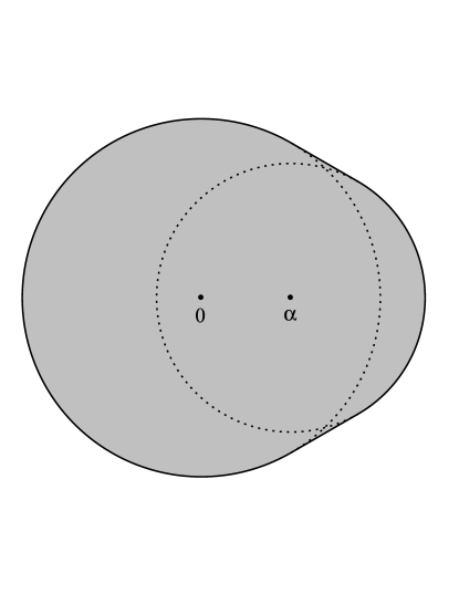
Figure 1. teardrop($\alpha$)

Drury’s theorem can now be stated as follows.

Theorem 4.1.

Let $T$ be an operator on a Hilbert space $H$ such that $W(T)\subset\overline{{\mathbb{D}}}$, and let $f:\overline{{\mathbb{D}}}\to\overline{{\mathbb{D}}}$ be a function in the disk algebra. Then

$$W(f(T))\subset\operatorname{teardrop}(f(0)).$$

This has the following immediate consequence.

Corollary 4.2.

Under the same hypotheses,

$$w(f(T))\leq 1+|f(0)|-|f(0)|^{2}\leq 5/4.$$

The rationale for these results, which also demonstrates their sharpness, is discussed by Drury in [6]. Our purpose here is to show how our results in the preceding sections fit into the proof of Theorem 4.1.

Following Drury, we define

$$Q(T,t,s):=I+t(T+T^{*})+sT^{*}T,$$

$$S:=\Bigl{\{}(t,s)\in{\mathbb{R}}^{+}\times{\mathbb{R}}:~{}w(T)\leq 1~{}\Rightarrow~{}Q(T,t,s)\geq 0\Bigr{\}}.$$

In a section entitled ‘the key issue’, Drury gives the following description of $S$.

Theorem 4.3.

The region $S$ is specified by the following inequalities:

$$\begin{cases}s\geq t^{2}-1/4,&\text{if~{}}0\leq t\leq 1/2,\\ s\geq 2t-1,&\text{if~{}}1/2\leq t\leq 1,\\ s\geq t^{2},&\text{if~{}}t\geq 1.\end{cases}$$

A picture of $S$ is given in Figure 2.

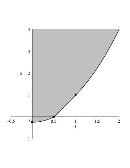
Figure 2. The region $S$

Proof.

We divide the argument into three cases, according to the value of $t$.

Case 1: $0\leq t\leq 1/2$. In this case, Theorem 3.2 shows that, if $s\geq t^{2}-1/4$, then, for all $T$ with $w(T)\leq 1$,

$$Q(T,t,s)\geq I+t(T+T^{*})+(t^{2}-1/4)T^{*}T\geq 0.$$

On the other hand, if $s<t^{2}-1/4$ and $T:=\begin{pmatrix}0&2\\ 0&0\end{pmatrix}$, then $w(T)\leq 1$ and

$$Q(T,t,s)=\begin{pmatrix}1&2t\\ 2t&1+4s\end{pmatrix}\not\geq 0,$$

because it has a negative determinant. Thus, for this range of values of $t$, we have $(t,s)\in S\iff s\geq t^{2}-1/4$.

Case 2: $1/2\leq t\leq 1$. In this case, if $s\geq 2t-1$, then, for all $T$ with $w(T)\leq 1$,

$$Q(T,t,s) \geq I+t(T+T^{*})+(2t-1)T^{*}T$$

$$=(1-t)(2I-(T+T^{*}))+(2t-1)(I+T)^{*}(I+T)\geq 0.$$

On the other hand, if $s<2t-1$ and $T:=-I$, then $w(T)\leq 1$ and

$$Q(T,t,s)=(1-2t+s)I\not\geq 0.$$

Therefore, for this range of values of $t$, we have $(t,s)\in S\iff s\geq 2t-1$.

Case 3: $t\geq 1$. In this case, if $s\geq t^{2}$, then, for all $T$ with $w(T)\leq 1$,

$$Q(T,t,s) \geq I+t(T+T^{*})+t^{2}T^{*}T$$

$$=(I+tT)^{*}(I+tT)\geq 0.$$

On the other hand, if $t\leq s<t^{2}$ and $T:=-(t/s)I$, then $w(T)\leq 1$ and

$$Q(T,t,s)=(1-t^{2}/s)I\not\geq 0.$$

Thus, for this range of values of $t$, we have $(t,s)\in S\iff s\geq t^{2}$. ∎

Remark.

The main novelty in the proof above is the use of Theorem 3.2 in Case 1, which shortens the argument considerably.

Proof of Theorem 4.1.

We follow the method of Drury, with a few details added.

Set $\alpha:=f(0)$. We can suppose that $|\alpha|<1$, otherwise $f$ is constant and the whole result becomes trivial. Let $\phi_{\alpha}$ be the disk automorphism defined by

$$\phi_{\alpha}(z):=\frac{\alpha+z}{1+\overline{\alpha}z},$$

and set $g:=\phi_{\alpha}^{-1}\circ f$. Then $g$ belongs to the disk algebra, $\|g\|_{\infty}\leq 1$ and $g(0)=0$. By Theorem 2.1 we have $W(g(T))\subset\overline{{\mathbb{D}}}$. Since $f=\phi_{\alpha}\circ g$, we may proceed by replacing $T$ by $g(T)$ and just studying the case $f=\phi_{\alpha}$. As $\phi_{\alpha}(T)=\phi_{|\alpha|}(e^{-i\arg\alpha}T)$, we may also assume that $\alpha\in[0,1)$.

Now $\operatorname{teardrop}(\alpha)$ is the intersection of the two families of half-planes

$$\{z:\operatorname{Re}(e^{-i\theta}z)\leq 1\}~{}~{}(\cos\theta\leq\alpha)\quad\text{and}\quad\{z:\operatorname{Re}(e^{-i\theta}(z-\alpha))\leq 1-\alpha^{2}\}~{}~{}(\cos\theta\geq\alpha).$$

So, to show $W(\phi_{\alpha}(T))\subset\operatorname{teardrop}(\alpha)$, it suffices to prove that

(4.1) $$\operatorname{Re}(e^{-i\theta}\phi_{\alpha}(T))\leq I\qquad(\cos\theta\leq\alpha)$$

and

(4.2) $$\operatorname{Re}(e^{-i\theta}(\phi_{\alpha}(T)-\alpha I))\leq(1-\alpha^{2})I\qquad(\cos\theta\geq\alpha).$$

We begin by proving (4.1). This inequality is equivalent to

$$2I-e^{-i\theta}\phi_{\alpha}(T)-e^{i\theta}\phi_{\alpha}(T^{*})\geq 0.$$

Given operators $A,B$ with $B$ invertible, we have $A\geq 0\iff B^{*}AB\geq 0$. Applying this with $A$ equal to the left-hand side above and $B:=(I+\alpha T)$, we see that the desired inequality is equivalent to

$$2(1-\alpha\cos\theta)I+(2\alpha-e^{i\theta}-\alpha^{2}e^{-i\theta})T+(2\alpha-e^{-i\theta}-\alpha^{2}e^{i\theta})T^{*}+2\alpha(\alpha-\cos\theta)T^{*}T\geq 0.$$

Set

$$\omega:=\frac{2\alpha-e^{i\theta}-\alpha^{2}e^{-i\theta}}{|2\alpha-e^{i\theta}-\alpha^{2}e^{-i\theta}|}=\frac{2\alpha-e^{i\theta}-\alpha^{2}e^{-i\theta}}{1-2\alpha\cos\theta+\alpha^{2}}.$$

Then we may rewrite the last inequality as

$$2(1-\alpha\cos\theta)I+(1-2\alpha\cos\theta+\alpha^{2})(\omega T+(\omega T)^{*})+2\alpha(\alpha-\cos\theta)(\omega T)^{*}(\omega T)\geq 0,$$

or equivalently, $Q(\omega T,t,s)\geq 0$, where

$$t:=\frac{1-2\alpha\cos\theta+\alpha^{2}}{2(1-\alpha\cos\theta)}\qquad\text{and}\qquad s:=\frac{\alpha(\alpha-\cos\theta)}{1-\alpha\cos\theta}=2t-1.$$

It is elementary to verify that, for $-1\leq\cos\theta\leq\alpha$, the parameter $t$ stays in the interval $[1/2,1]$. Hence, by Theorem 4.3, we do indeed have $Q(\omega T,t,s)\geq 0$. This establishes (4.1).

Now we turn to (4.2). This inequality is equivalent to

$$2I-e^{-i\theta}\psi_{\alpha}(T)-e^{i\theta}\psi_{\alpha}(T^{*})\geq 0,$$

where $\psi_{\alpha}(z):=z/(1+\alpha z)$. As before, considering $B^{*}AB$ with $B:=(I+\alpha T)$, we see that the preceding inequality is equivalent to

$$2I+(2\alpha-e^{-i\theta})T+(2\alpha-e^{i\theta}T^{*})+2\alpha(\alpha-\cos\theta)T^{*}T\geq 0.$$

Set

$$\omega:=\frac{2\alpha-e^{-i\theta}}{|2\alpha-e^{-i\theta}|}=\frac{2\alpha-e^{-i\theta}}{2\sqrt{\alpha(\alpha-\cos\theta)+1/4}}.$$

Then we may rewrite the last inequality as

$$I+\sqrt{\alpha(\alpha-\cos\theta)+1/4}\bigl{(}\omega T+(\omega T)^{*}\bigr{)}+\alpha(\alpha-\cos\theta)(\omega T)^{*}(\omega T)\geq 0,$$

or equivalently, $Q(\omega T,t,s)\geq 0$, where

$$t:=\sqrt{\alpha(\alpha-\cos\theta)+1/4}\qquad\text{and}\qquad s:=\alpha(\alpha-\cos\theta)=t^{2}-1/4.$$

It is elementary to verify that, for $\alpha\leq\cos\theta\leq 1$, the parameter $t$ stays in the interval $[0,1/2]$. Hence, by Theorem 4.3, we do indeed have $Q(\omega T,t,s)\geq 0$. This establishes (4.2), and completes the proof. ∎

Remark.

The part of the numerical range of $f(T)$ ‘sticking out’ of the unit disk is governed by the inequality (4.2), which corresponds to the slice of $S$ where $0\leq t\leq 1/2$, which is in turn determined by the operator inequality Theorem 3.2.

5. Concluding remarks

5.1. Aleksandrov–Clark measures

Lemma 2.3 is a special case of a construction of Clark later generalized by Aleksandrov. Let $f:{\mathbb{D}}\to{\mathbb{D}}$ be holomorphic with $f(0)=0$. Then, given $\gamma\in{\mathbb{T}}$, there exists a probability measure $\mu_{\gamma}$ on ${\mathbb{T}}$ such that

(5.1) $$\frac{1}{1-\overline{\gamma}f(z)}=\int_{{\mathbb{T}}}\frac{d\mu_{\gamma}(\zeta)}{1-\overline{\zeta}z}\qquad(z\in{\mathbb{D}}).$$

The measures $\mu_{\gamma}$ are known as Aleksandrov–Clark measures. For details of their construction and an account of their properties, see for example [11] and [12].

It is possible to base a proof of Theorem 2.1 directly on the formula (5.1). Indeed, a proof very similar to this appears in the paper of Kato [9].

5.2. Reformulations of the inequality (3.1)

The inequality (3.1) can be reformulated in various equivalent ways. We record two of them here.

Proposition 5.1.

Let $T$ be an operator on a Hilbert space $H$ and let $x\in H$. If $w(T)\leq 1$ and $\|x\|\leq 1$, then

(5.2) $$\|Tx\|\leq\max\Bigl{\{}2|\sin\theta|,\sqrt{2}\Bigr{\}},$$

where $\theta$ is the hermitian angle between $x$ and $Tx$.

Proof.

By definition of hermitian angle, $|\langle Tx,x\rangle|=\|Tx\|\|x\|\cos\theta$. We can suppose that $\|x\|=1$. Substituting into (3.1), we get $\|Tx\|^{2}-2\leq 2\sqrt{1-\|Tx\|^{2}\cos^{2}\theta}$. If $\|Tx\|^{2}\geq 2$, then we may square both sides to obtain

$$\|Tx\|^{4}-4\|Tx\|^{2}+4\leq 4-4\|Tx\|^{2}\cos^{2}\theta,$$

which leads to $\|Tx\|\leq 2|\sin\theta|$. On the other hand, if $\|Tx\|^{2}<2$, then obviously $\|Tx\|<\sqrt{2}$. Either way, (5.2) holds. ∎

Proposition 5.2.

If the matrix $\begin{pmatrix}a&b\\ c&d\end{pmatrix}$ has numerical radius at most $1$, then

$$|c|\leq 1+\sqrt{1-|a|^{2}}.$$

Proof.

Applying Theorem 3.1 with $H={\mathbb{C}}^{2}$ and $x=(1,0)$, we obtain

$$|a|^{2}+|c|^{2}\leq 2+2\sqrt{1-|a|^{2}}.$$

After simplification, this gives the result. ∎

We mention in passing that there are complete characterizations of operators $T$ such that $w(T)\leq 1$; see Ando [1].

5.3. Extension to general domains

The papers [3] and [9] contain some partial extensions of Theorem 2.1 to certain domains other than the disk.

More recently, Crouzeix [4] has shown that, if $T$ is any Hilbert-space operator and $f$ is holomorphic on a neighborhood of $\overline{W(T)}$, then

(5.3) $$\|f(T)\|\leq C\sup_{z\in W(T)}|f(z)|,$$

where $C$ is an absolute constant satisfying $C\leq 11.08$. It is conjectured that (5.3) holds with $C=2$. This is best possible, as can be seen by considering the matrix

(5.4) $$T=\begin{pmatrix}0&2\\ 0&0\end{pmatrix},$$

which satisfies $W(T)=\overline{{\mathbb{D}}}$ and $\|T\|=2$.

Of course inequality (5.3) implies the numerical-range mapping inequality

(5.5) $$w(f(T))\leq C\sup_{z\in W(T)}|f(z)|.$$

However, in the light of Corollary 4.2, it is conceivable that the best constant $C$ in (5.5) is actually smaller than $2$. The best that we can hope for is $C=5/4$. Indeed, taking $T$ as in (5.4) and $f(z):=(1-2z)/(2-z)$, we have

$$\sup_{z\in W(T)}|f(z)|=\sup_{z\in\overline{{\mathbb{D}}}}\Bigl{|}\frac{1-2z}{2-z}\Bigr{|}=1,$$

while $f(T)=I/2-3T/4$, which has numerical range $\overline{D}(1/2,3/4)$, so $w(f(T))=5/4$.

References

- [1] T. Ando, ‘Structure of operators with numerical radius one’, Acta Sci. Math. (Szeged) 34 (1973), 11–15.
- [2] C. A. Berger, ‘A strange dilation theorem’, Abstract 625–152, Notices Amer. Math. Soc. 12 (1965), 590.
- [3] C. A. Berger, J. G. Stampfli, ‘Mapping theorems for the numerical range’, Amer. J. Math. 89 (1967), 1047–1055.
- [4] M. Crouzeix, ‘Numerical range and functional calculus in Hilbert space’, J. Funct. Anal. 244 (2007), 668–690.
- [5] M. A. Dritschel, H. J. Woerdeman, ‘Model theory and linear extreme points in the numerical radius ball’, Mem. Amer. Math. Soc. 129 (1997), viii+62 pp.
- [6] S. W. Drury, ‘Symbolic calculus of operators with unit numerical radius’, Lin. Alg. Appl. 428 (2008), 2061–2069.
- [7] J. B. Garnett, Bounded Analytic Functions, Revised first edition. Springer, New York, 2007.
- [8] K. E. Gustafson, D. K. M. Rao, Numerical Range. The Field of Values of Linear Operators and Matrices, Springer-Verlag, New York, 1997.
- [9] T. Kato, ‘Some mapping theorems for the numerical range’, Proc. Japan Acad. 41 (1965), 652–655.
- [10] C. Pearcy, ‘An elementary proof of the power inequality for the numerical radius’, Michigan Math. J. 13 (1966), 289–291.
- [11] A. Poltoratski, D. Sarason, ‘Aleksandrov-Clark measures’, in Recent Advances in Operator-related Function Theory, 1–14, Contemp. Math. 393, Amer. Math. Soc., Providence, RI, 2006.
- [12] E. Saksman, ‘An elementary introduction to Clark measures’, in Topics in Complex Analysis and Operator Theory, 85–136, Univ. Málaga, Málaga, 2007.