Type-Directed Synthesis of Products
Princeton University Master’s Thesi-s

TYPE DIRECTED SYNTHESIS OF PRODUCTS
Jonathan Frankle
A THESIS
PRESENTED TO THE FACULTY
OF PRINCETON UNIVERSITY
IN CANDIDACY FOR THE DEGREE
OF MASTER OF SCIENCE IN ENGINEERING
RECOMMENDED FOR ACCEPTANCE
BY THE DEPARTMENT OF
COMPUTER SCIENCE
Adviser: David Walker
September 2015

© Copyright by Jonathan Frankle, 2015. All rights reserved.

Abstract

Software synthesis - the process of generating complete, general-purpose programs from specifications - has become a hot research topic in the past few years. For decades the problem was thought to be insurmountable: the search space of possible programs is far too massive to efficiently traverse. Advances in efficient constraint solving have overcome this barrier, enabling a new generation of effective synthesis systems. Most existing systems compile synthesis tasks down to low-level SMT instances, sacrificing high-level semantic information while solving only first-order problems (i.e., filling integer holes). Recent work takes an alternative approach, using the Curry-Howard isomorphism and techniques from automated theorem proving to construct higher-order programs with algebraic datatypes.

My thesis involved extending this type-directed synthesis engine to handle product types, which required significant modifications to both the underlying theory and the tool itself. Product types streamline other language features, eliminating variable-arity constructors among other workarounds employed in the original synthesis system. A form of logical conjunction, products are invertible, making it possible to equip the synthesis system with an efficient theorem-proving technique called focusing that eliminates many of the nondeterministic choices inherent in proof search. These theoretical enhancements informed a new version of the type-directed synthesis prototype implementation, which remained performance-competitive with the original synthesizer. A significant advantage of the type-directed synthesis framework is its extensibility; this thesis is a roadmap for future such efforts to increase the expressive power of the system.

1 Introduction

Since the advent of computer programming, the cycle of writing, testing, and debugging code has remained a tedious and error-prone undertaking. There is no middle ground between a program that is correct and one that is not, so software development demands often-frustrating levels of precision. The task of writing code is mechanical and repetitive, with boilerplate and common idioms consuming ever more valuable developer-time. Aside from the languages and platforms, the process of software engineering has changed little over the past four decades.

The discipline of software synthesis responds to these deficiencies with a simple question: if computers can automate so much of our everyday lives, why can they not do the same for the task of developing software? Outside of a few specialized domains, this question – until recently – had an equally simple answer: the search space of candidate programs is too large to explore efficiently. As we increase the number of abstract syntax tree (AST) nodes that a program might require, the search space explodes combinatorially. Synthesizing even small programs seems hopeless.

In the past decade, however, several research program analysis and synthesis systems have overcome these barriers and developed into useful programming tools. At the core of Sketch [13], Rosette [22, 23], and Leon [9] are efficient SAT and SMT-solvers. These tools automate many development tasks – including test case generation, verification, angelic nondeterminism, and synthesis [22] – by compiling programs into constraint-solving problems.

These synthesis techniques, while a major technological step forward, are still quite limited. Constraint-solving tasks are fundamentally first-order: although they efficiently fill integer and boolean holes, they cannot scale to higher-order programs. Furthermore, in the process of compiling synthesis problems into the low-level language of constraint-solvers, these methods sacrifice high-level semantic and type information that might guide the synthesis procedure through the search space more efficiently.

Based on these observations, recent work by Steve Zdancewic and Peter-Michael Osera at the Univerity of Pennsylvania [14] explores a different approach to synthesis: theorem-proving. The Curry-Howard isomorphism permits us to treat the type of a desired program as a theorem whose proof is the synthesized program. Translating this idea into an algorithm, we can search for the solution to the synthesis problem using existing automated theorem-proving techniques. Since many programs inhabit the same type, users also provide input-output examples to better specify the desired function and constrain the synthesizer’s result.

This type-directed approach scales to higher-order programs and preserves the high-level program structures that guide the synthesis process. The synthesis algorithm can be designed to search only for well-typed programs in normal form, drastically reducing the search space of possible ASTs. At the time of writing, both of these features are unique to type-directed synthesis.

Not only is this technique efficient, but it also has the ability to scale to language features that have, until now, remained beyond the reach of synthesis. Many desirable features, like file input-output, map to existing systems of logic that, when integrated into the synthesizer, instantly enable it to generate the corresponding programs. For example, one might imagine synthesizing effectful computation using monads by performing proof search in lax logic [16]. When these logical constructs are kept orthogonal to one another, features can be added and removed from the synthesis language in modular fashion. This extensibility is one of the most noteworthy benefits of type-directed synthesis.

This thesis represents the first such extension to the type-directed synthesis system. My research involved adding product types to the original synthesis framework, which until then captured only the simply typed lambda calculus with recursion and algebraic datatypes. In the process, I heavily revised and expanded both the formal judgments that govern the synthesis procedure and the code that implements it, integrating additional theorem proving techniques that pave the way for future language extensions.

Contributions of this thesis.

1. An analysis of the effect of searching only for typed programs or typed programs in normal form on the size of the number of programs at a particular type.

2. A revised presentation of the judgments for the original type-directed synthesis system.

3. An extension of the original synthesis judgments to include product types and the focusing technique.

4. Theorems about the properties of the updated synthesis judgments and focusing, including proofs of admissibility of focusing and soundness of the full system.

5. Updates to the type-directed synthesis prototype that implement the new judgments.

6. An evaluation of the performance of the updated implementation on several canonical programs involving product types.

7. A thorough survey of related work.

8. A discussion of future research avenues for type-directed synthesis with emphasis on the observation that examples are refinement types.

Overview.

The body of this thesis is structured as follows: I begin with an in-depth look at the original type-directed synthesis system in Section 2. In Section 3, I introduce the theory underlying synthesis of products and extensively discuss the focusing technique, which handles product types efficiently. I describe implementation changes made to add tuples to the synthesis framework and evaluate the performance of the modified system in Section 4. In Section 5, I discuss related work, including extended summaries of other synthesis systems. Finally, I outline future research directions in Section 6, with particular emphasis on using intersection and refinement types that integrate input-output examples into the type system. I conclude in Section 7. Proofs of theorems presented throughout this thesis appear in Appendix A.

2 Type-Directed Synthesis

2.1 Overview

The following is a brief summary of type-directed synthesis [14], presented loosely within the Syntax-Guided Synthesis [3] framework.

Background theory.

The system synthesizes over the simply-typed lambda calculus with recursive functions and non-polymorphic algebraic datatypes. In practice, it uses a subset of OCaml with the aforementioned features. In order to guarantee that all programs terminate, the language permits only structural recursion. Pre-defined functions can be made available to the synthesis process if desired (i.e., providing map and fold to a synthesis task involving list manipulation).

Synthesis problem.

A user specifies the name and type signature of a function to be synthesized. No additional structural guidance or “sketching” is provided.

Solution specification.

The function’s type information combined with input-output examples constrain the function to be synthesized. We can treat this set of examples as a partial function that we wish to generalize into a total function. Since type-directed synthesis aims to scale to multi-argument, higher-order functions, these examples can map multiple inputs, including other functions, to a single output. Functions are not permissible as output examples, however, since the synthesis procedure must be able to decidably test outputs for equality.

Optimality criterion.

The synthesis problem as currently described lends itself to a very simple algorithm: create a function that (1) on an input specified in an example, supplies the corresponding output and (2) on all other inputs, returns an arbitrary, well-typed value. To avoid generating such useless, over-fitted programs, type-directed synthesis requires some notion of a best result. In practice, we create the smallest (measured in AST nodes) program that satisfies the specification, since a more generic, recursive solution will lead to a smaller program than one that merely matches on examples.

Search strategy.

Type-directed synthesis treats the signature of the function in the synthesis problem as a theorem to be proved and uses a modified form of reverse proof search [15] that integrates input-output examples to generate a program. By the Curry-Howard isomorphism, a proof of the theorem is a program with the desired type; if it satisfies the input-output examples, then it is a solution to the overall synthesis problem.

Style.

Type-directed synthesis can be characterized as a hybrid algorithm that has qualities of both deductive and inductive synthesis. It uses a set of rules to extract the structure of the input-output examples into a program, which is reminiscent of deductive synthesis algorithms that use a similar process on complete specifications. When guessing variables and function applications, however, type-directed synthesis generates terms and checks whether they satisfy the examples, an approach in the style of inductive strategies like CEGIS [20].

Description	(a)  Initial synthesis problem.	(b)  Synthesize a function.
Program	len : natlist -> nat = ?	len (ls : natlist) : nat = ?
Examples	5cm ?:$\langle$$\cdot$; []     => 0$\rangle$
?:$\langle$$\cdot$; [3]    => 1$\rangle$
?:$\langle$$\cdot$; [4; 3] => 2$\rangle$	6cm ?:$\langle$len = ..., ls =     []; 0$\rangle$
?:$\langle$len = ..., ls =    [3]; 1$\rangle$
?:$\langle$len = ..., ls = [4; 3]; 2$\rangle$
Judgment		IRefine-Fix

(c)  Synthesize a match statement.	(d)  Complete the Nil branch with the O constructor.
8cm len (ls : natlist) : nat =
2emmatch ls with
2em| Nil          -> ?1
2em| Cons(hd, tl) -> ?2	8cm len (ls : natlist) : nat =
2emmatch ls with
2em| Nil          -> O
2em| Cons(hd, tl) -> ?2
9cm ?1:$\langle$len = ..., ls =     []                  ; 0$\rangle$
?2:$\langle$len = ..., ls =    [3], hd = 3, tl =  []; 1$\rangle$
?2:$\langle$len = ..., ls = [4; 3], hd = 4, tl = [3]; 2$\rangle$	9cm ?2:$\langle$len = ..., ls =    [3], hd = 3, tl =  []; 1$\rangle$
?2:$\langle$len = ..., ls = [4; 3], hd = 4, tl = [3]; 2$\rangle$
IRefine-Match, EGuess-Ctx	IRefine-Ctor

(e)  Synthesize constructor S in the remaining branch.	(f)  Synthesize an application to fill the final hole.
8cm len (ls : natlist) : nat =
2emmatch ls with
2em| Nil          -> O
2em| Cons(hd, tl) -> S(?2)	8cm len (ls : natlist) : nat =
2emmatch ls with
2em| Nil          -> O
2em| Cons(hd, tl) -> S(len tl)
9cm ?2:$\langle$len = ..., ls =    [3], hd = 3, tl =  []; 0$\rangle$
?2:$\langle$len = ..., ls = [4; 3], hd = 4, tl = [3]; 1$\rangle$	8cm
IRefine-Ctor	IRefine-Guess, EGuess-App, EGuess-Ctx

Figure 1: A step-by-step derivation of the list length function in type-directed synthesis. A ? character refers to a hole in the program that the synthesis algorithm aims to fill. Each example world, delimited with $\langle$ and $\rangle$, contains variable bindings to the left of the ; and the goal value to the right. The preceding ? indicates the hole to which the example world corresponds. For brevity, we write unary numbers in their Arabic equivalents (S (S (O)) is abbreviated as 2) and lists in equivalent OCaml syntax (Cons(2, Cons(1, Nil)) is [2; 1]). The names of all recursive functions in scope (in this case len) are always available in the list of variable bindings. They are bound to the partial functions comprising their definitions. The example for len is the initial partial function example at the beginning of the synthesis process; it is elided from the example worlds for space.

2.2 Case Study: List length

Before delving into the technical details of the theory, consider the process of synthesizing the list length function as illustrated in Figure 2.1.

In Figure 1a, we begin with our synthesis problem: a function with its type signature and a list of input-output examples. The ? preceding each example represents the hole to which the example corresponds. Initially, the entire function to be synthesized comprises a single hole.

Enclosed within angle brackets is each example world, which we define as a pair of (1) bindings of names to values and (2) the goal value that should be taken on by the expression chosen to fill the hole when the names are bound to those values. For example, we can read the expression

?₁: $\langle$x = 1, y = 2; 5$\rangle$

as

When x = 1 and y = 2, the expression synthesized to fill hole ?₁ should evaluate to 5.

In our initial synthesis problem in Figure 1a, no names have yet been bound to values. We could imagine providing the synthesis instance with a library of existing functions, like fold and map, in which case our example worlds would contain already-bound names at the start of the synthesis process.

Each goal value is expressed as a partial function mapping input arguments to an output. For example,

[1; 2] => inc => [2; 3]

means that, on inputs [1; 2] and the increment function, the desired output is [2; 3].

In Figure 1b, we observe that every example is a partial function mapping a natlist to a nat and, as such, we synthesize a function with a natlist argument called ls. We must update our examples in kind. Where before we had an example world of the form

$\langle\cdot$; [4; 3] => 2$\rangle$

we now extract the value of ls and move it to the list of names bound to values:

$\langle$ls = [4; 3]; 2$\rangle$

Since we have now synthesized a function, our hole is of type nat and the goal value is the remainder of the partial function with ls removed.

In Figure 1c, we synthesize a match statement to break down the structure of ls. This creates two holes, one for each branch of the match statement. We partition our set of examples between the two holes depending on the constructor of the value bound to ls. Those examples for which ls = [] constrain the hole for the Nil branch; all other examples constrain the Cons branch.

In Figure 1d, we turn our attention to the Nil branch. Since we only have a single example, it is safe to simply synthesize the value in the example’s goal position (namely the constructor O). In the other branch, too, every example has the same constructor (S), which we then generate in our program (Figure 1e). We update the value in the goal position accordingly, removing one use of the S constructor. Finally, with a recursive call to len on tl, our function is complete.

It is important to note that every function we generate is recursive. Therefore, the name of each function, including the top-level function of the synthesis problem, is available in every example world for which it is in scope. Function names are bound to the partial functions comprising their examples. Making these names available allows for recursive function calls. The examples for len are elided from example worlds in Figure 1 for readability.

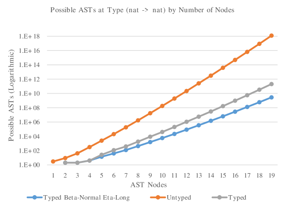
Figure 2: The number of possible ASTs (at type nat $\rightarrow$ nat) with a particular number of nodes. ASTs were generated over the type-directed synthesis language (the lambda calculus with recursive functions and algebraic datatypes). The top line (orange) includes all possible ASTs, while the middle and bottom lines include only typed (grey) and typed beta-normal eta-long (blue) ASTs respectively. The scale on the vertical axis is logarithmic.

$\tau$	$::=~{}$$\mathcal{B}$$~{}|~{}$${\tau_{1}}\rightarrow{\tau_{2}}$	(Types: base types and function types)
$v$	$::=~{}$$C$ $({{v}_{1}{,}~{}...{,}~{}{v}_{m}})$ 1em$~{}|~{}$$\mathsf{fix}~{}{f}{({x}:{\tau_{1}})}:{\tau_{2}}={e}$$~{}|~{}$$pf$	(Values: constructors, functions, and partial functions)
$pf$	$::=~{}$$\overline{{v_{i}\Rightarrow\epsilon_{i}}}^{i\in m}$	(Partial functions: a finite map from inputs to outputs)
$\epsilon$	$::=~{}$$C$ $({{\epsilon}_{1}{,}~{}...{,}~{}{\epsilon}_{m}})$ $~{}|~{}$$pf$	(Examples)
$e$	$::=~{}$$x$$~{}|~{}$$C$ $({{e}_{1}{,}~{}...{,}~{}{e}_{m}})$ $~{}|~{}$$pf$ 1em$~{}|~{}$$\mathsf{fix}~{}{f}{({x}:{\tau_{1}})}:{\tau_{2}}={e}$$~{}|~{}$${e_{1}}~{}{e_{2}}$ 1em$~{}|~{}$$\mathsf{match}~{}{e}~{}\mathsf{with}~{}{\overline{{C_{i}~{}({{x}_{1}{,}~{}...{,}~{}{x}_{m}})\rightarrow e_{i}}}^{i\in l}}$	(Expressions)
$E$	$::=~{}$$x$$~{}|~{}$${E}~{}{I}$	(Elimination forms)
$I$	$::=~{}$$E$$~{}|~{}$$C$ $({{I}_{1}{,}~{}...{,}~{}{I}_{m}})$ 1em$~{}|~{}$$\mathsf{fix}~{}{f}{({x}:{\tau_{1}})}:{\tau_{2}}={I}$ 1em$~{}|~{}$$\mathsf{match}~{}{E}~{}\mathsf{with}~{}{\overline{{C_{i}~{}({{x}_{1}{,}~{}...{,}~{}{x}_{m}})\rightarrow I_{i}}}^{i\in l}}$	(Introduction forms)
$\Sigma$	$::=~{}$$\cdot$$~{}|~{}$$\Sigma$, ${C}:{{\tau_{1}*...*\tau_{n}}\rightarrow\mathcal{B}}$	(Constructor context: a map from constructor names to types)
$\Gamma$	$::=~{}$$\cdot$$~{}|~{}$$\Gamma$, ${x}:{\tau}$	(Type context: bindings of names to types)
$\mathcal{E}$	$::=~{}$$\cdot$$~{}|~{}$$\mathcal{E}$, ${x}\triangleright{\epsilon}$	(Example context: names refined by examples)
$w$	$::=~{}$$\langle{\mathcal{E}};{\epsilon}\rangle$	(A single world: an example context and result example)
$\mathcal{W}$	$::=~{}$$\cdot$$~{}|~{}$$\mathcal{W}$, $w$	(A set of worlds)

Figure 3: Grammars for the synthesis judgments of type-directed synthesis.

$$\boxed{{{\Sigma}~{}|~{}{\Gamma}~{}|~{}{\mathcal{W}}}\vdash{\tau}\overset{I}{\leadsto}{I}missing}$$

IRefine-Guess $$\displaystyle{\hbox{\hskip 67.44533pt\vbox{\hbox{\hskip-67.44531pt\hbox{\hbox{$\displaystyle\displaystyle{{\Sigma}~{}|~{}{\Gamma}}\vdash{\mathcal{B}}\overset{E}{\leadsto}{E}$}\hskip 16.00003pt\hbox{\hbox{$\displaystyle\displaystyle\forall i\in n,~{}\mathcal{E}_{i}(E)\rightarrow^{*}\epsilon_{i}$}}}}\vbox{}}}\over\hbox{\hskip 38.2486pt\vbox{\vbox{}\hbox{\hskip-38.24858pt\hbox{\hbox{$\displaystyle\displaystyle{{\Sigma}~{}|~{}{\Gamma}~{}|~{}{\overline{{\langle{\mathcal{E}_{i}};{\epsilon_{i}}\rangle}}^{i\in n}}}\vdash{\mathcal{B}}\overset{I}{\leadsto}{E}$}}}}}} \displaystyle{\hbox{\hskip 92.9936pt\vbox{\hbox{\hskip-92.9936pt\hbox{\hbox{$\displaystyle\displaystyle{C}:{{\tau_{1}*...*\tau_{m}}\rightarrow{\mathcal{B}}}\in\Sigma$}\hskip 16.00003pt\hbox{\hbox{$\displaystyle\displaystyle\forall j\in m,{{\Sigma}~{}|~{}{\Gamma}~{}|~{}{\overline{{\langle{\mathcal{E}_{i}};{\epsilon_{(i,j)}}\rangle}}^{i\in n}}}\vdash{\tau_{j}}\overset{I}{\leadsto}{I_{j}}$}}}}\vbox{}}}\over\hbox{\hskip 61.43736pt\vbox{\vbox{}\hbox{\hskip-61.43736pt\hbox{\hbox{$\displaystyle\displaystyle{{\Sigma}~{}|~{}{\Gamma}~{}|~{}{\overline{{\langle{\mathcal{E}_{i}};{{C}~{}{(\epsilon_{(i,1)},...,I_{(i,m)})}}\rangle}}^{i\in n}}}\vdash{\mathcal{B}}\overset{I}{\leadsto}{{C}~{}{({{I}_{1}{,}~{}...{,}~{}{I}_{m}})}}$}}}}}}$$                IRefine-Ctor

IRefine-Fix $$\displaystyle{\hbox{\hskip 65.93805pt\vbox{\hbox{\hskip-65.93803pt\hbox{\hbox{$\displaystyle\displaystyle{{\Sigma}~{}|~{}{\Gamma,{f}:{{\tau_{1}}\rightarrow{\tau_{2}}},{x}:{\tau_{1}}}~{}|~{}{\overline{{\langle{\mathcal{E}_{i},{f}\triangleright{\overline{{v_{(i,j)}\Rightarrow\epsilon_{(i,j)}}}^{j\in m_{i}}},{x}\triangleright{v_{(i,k)}}};{\epsilon_{(i,k)}}\rangle}}^{(i,k)\in(n,m_{i})}}}\vdash{\tau_{2}}\overset{I}{\leadsto}{I}$}}}\vbox{}}}\over\hbox{\hskip 71.11897pt\vbox{\vbox{}\hbox{\hskip-71.11896pt\hbox{\hbox{$\displaystyle\displaystyle{{\Sigma}~{}|~{}{\Gamma}~{}|~{}{\overline{{\langle{\mathcal{E}_{i}};{\overline{{v_{(i,j)}\Rightarrow\epsilon_{(i,j)}}}^{j\in m_{i}}}\rangle}}^{i\in n}}}\vdash{{\tau_{1}}\rightarrow{\tau_{2}}}\overset{I}{\leadsto}{\mathsf{fix}~{}{f}{({x}:{\tau_{1}})}:{\tau_{2}}={I}}$}}}}}}$$

IRefine-Match $$\displaystyle{\hbox{\hskip 162.14134pt\vbox{\hbox{\hskip-90.91315pt\hbox{\hbox{$\displaystyle\displaystyle{{\Sigma}~{}|~{}{\Gamma}}\vdash{\mathcal{B}}\overset{E}{\leadsto}{E}$}\hskip 16.00003pt\hbox{\hbox{$\displaystyle\displaystyle\forall j\in m,~{}{C_{j}}:{{\tau_{(j,1)}*...*\tau_{(j,l)}}\rightarrow{\mathcal{B}}}\in\Sigma$}}}}\vbox{\hbox{\hskip-162.14134pt\hbox{\hbox{$\displaystyle\displaystyle\forall j\in m,~{}{{\Sigma}~{}|~{}{\Gamma,{x}:{\tau_{(j,1)}},...,{x}:{\tau_{(j,l)}}}~{}|~{}{\{\langle{\mathcal{E}_{i},{x_{1}}\triangleright{v_{1}},...,{x_{l}}\triangleright{v_{l}}};{\epsilon_{i}}\rangle~{}\big{|}~{}\mathcal{E}_{i}(E)\rightarrow^{*}C_{j}~{}(v_{1},...,v_{l})\}}}\vdash{\tau}\overset{I}{\leadsto}{I_{j}}$}}}\vbox{}}}}\over\hbox{\hskip 66.72614pt\vbox{\vbox{}\hbox{\hskip-66.72612pt\hbox{\hbox{$\displaystyle\displaystyle{{\Sigma}~{}|~{}{\Gamma}~{}|~{}{\overline{{\langle{\mathcal{E}_{i}};{\epsilon_{i}}\rangle}}^{i\in n}}}\vdash{\tau}\overset{I}{\leadsto}{\mathsf{match}~{}{E}~{}\mathsf{with}~{}{\overline{{C_{j}~{}(x_{1},...,x_{l})\rightarrow I_{j}}}^{j\in m}}}$}}}}}}$$

$$\boxed{{{\Sigma}~{}|~{}{\Gamma}}\vdash{\tau}\overset{E}{\leadsto}{E}}$$

EGuess-Ctx $$\displaystyle{\hbox{\hskip 11.42363pt\vbox{\hbox{\hskip-11.42363pt\hbox{\hbox{$\displaystyle\displaystyle{x}:{\tau}\in\Gamma$}}}\vbox{}}}\over\hbox{\hskip 25.71536pt\vbox{\vbox{}\hbox{\hskip-25.71535pt\hbox{\hbox{$\displaystyle\displaystyle{{\Sigma}~{}|~{}{\Gamma}}\vdash{\tau}\overset{E}{\leadsto}{x}$}}}}}} \displaystyle{\hbox{\hskip 73.65552pt\vbox{\hbox{\hskip-73.6555pt\hbox{\hbox{$\displaystyle\displaystyle{{\Sigma}~{}|~{}{\Gamma}}\vdash{{\tau_{1}}\rightarrow{\tau}}\overset{E}{\leadsto}{E}$}\hskip 16.00003pt\hbox{\hbox{$\displaystyle\displaystyle{{\Sigma}~{}|~{}{\Gamma}~{}|~{}{\cdot}}\vdash{\tau_{1}}\overset{I}{\leadsto}{I}$}}}}\vbox{}}}\over\hbox{\hskip 30.01677pt\vbox{\vbox{}\hbox{\hskip-30.01677pt\hbox{\hbox{$\displaystyle\displaystyle{{\Sigma}~{}|~{}{\Gamma}}\vdash{\tau}\overset{E}{\leadsto}{{E}~{}{I}}$}}}}}}$$                      EGuess-App

Figure 4: Synthesis judgments for type-directed synthesis. An expression with a bar and an index above it represents a set of expressions sharing the same structure.

2.3 Proof Search

Search strategy.

The primary distinguishing quality of type-directed synthesis is its search strategy. The grammar of expressions $e$ in the background theory is specified in Figure 3. Within this grammar are myriad ASTs that are not well-typed. As Figure 2 illustrates, merely restricting our search to well-typed terms drastically decreases the size of the search space. Even amongst well-typed terms, there are numerous expressions that are functionally identical. For example, ${(\mathsf{fix}~{}{f}{({x}:{\tau_{1}})}:{\tau_{1}}={x})}~{}{1}$ beta-reduces to 1 and $\mathsf{fix}~{}{f}{({x}:{\tau_{1}})}:{\tau_{2}}={({g}~{}{x})}$ eta-reduces to $g$. If we confine our search to programs in eta-long, beta-normal form, we avoid considering some of these duplicates and further reduce our search space. Figure 2 demonstrates the benefit of this further restriction: an additional one to two orders of magnitude reduction in the size of the search space.

Based on these observations, type-directed syntax avoids searching amongst all expressions ($e$), instead generating well-typed ASTs over a more restrictive grammar: that of introduction ($I$) and elimination ($E$) forms. Doing so guarantees that programs synthesized are in beta-normal form, since no lambda term can appear on the left side of an application. If, in addition, we generate only lambdas at function type, programs will also be eta-long.

We can combine these ideas into a proof search algorithm that begins with a synthesis problem as in Figure 1 and uses type information, along with the structure of examples, to generate programs. The synthesis judgments for this algorithm appear in Figure 4.

Refining introduction forms.

The judgment for producing introduction forms, which is also the top-level synthesis judgment, is of the form

${{\Sigma}~{}|~{}{\Gamma}~{}|~{}{\mathcal{W}}}\vdash{\tau}\overset{I}{\leadsto}{I}$

which states:

Given constructors $\Sigma$ and names bound to types $\Gamma$, we synthesize introduction form $I$ at type $\tau$ conforming to the examples in worlds $\mathcal{W}$.

The IRefine-Fix rule extracts the structure of a partial function example as in Figure 1b, synthesizing a fixpoint and creating a new subproblem for the fixpoint’s body that can refer to the argument and make recursive calls. The IRefine-Ctor rule observes that every example shares the same constructor and therefore synthesizes the constructor in the program, likewise creating subproblems for each of the constructor’s arguments.

The IRefine-Match rule generates a match statement, guessing an elimination-form scrutinee at base type on which to pattern-match. The rule creates a sub-problem for each branch of the match statement - that is, one for every constructor of the scrutinee’s type. The existing set of examples is partitioned among these sub-problems according to the value that the scrutinee takes on when evaluated in each example world. Since the values of the bound variables may vary from world to world, the scrutinee can evaluate to different constructors in different contexts. This evaluation step determines which examples correspond to which branches, allowing us to constrain the sub-problems and continue with the synthesis process.

Finally, at base type ($\mathcal{B}$), we may also guess an elimination form, captured by the IRefine-Guess rule. The restriction that this only occurs at base type helps enforce the property that we only generate eta-long programs.

Guessing elimination forms.

The judgment form for guessing elimination forms

${{\Sigma}~{}|~{}{\Gamma}}\vdash{\tau}\overset{E}{\leadsto}{E}$

states:

Given constructors $\Sigma$ and names bound to types $\Gamma$, we synthesize elimination form $E$ at type $\tau$.

Observe that this judgment form does not include examples. Unlike the introduction forms, we cannot use the structural content of the examples to inform the elimination forms we guess. Instead, we may only ensure that the elimination form that we generate obeys the examples. This requirement appears in the additional condition of the IRefine-Guess rule

$\forall i\in n,~{}\mathcal{E}_{i}(E)\rightarrow^{*}\epsilon_{i}$

reading:

For each of our $n$ examples, the elimination form $E$ must, when substituted with the value bindings in $\mathcal{E}_{i}$, evaluate to the corresponding goal value $\epsilon_{i}$.

The EGuess-App rule guesses a function application by recursively guessing a function and an argument. The function must be an elimination form, which ensures that we only guess beta-normal programs. The argument may be an introduction form, but the call back into an IRefine rule does so without examples. Finally, the base case EGuess-Ctx guesses a name from the context $\Gamma$.

Nondeterminism.

These rules are highly nondeterministic: at any point, several rules apply. This is especially pertinent at base type, where we could refine a constructor or match statement while guessing an elimination form. Figure 1 traces only one of many paths through the expansive search space that this nondeterminism creates.

Nondeterminism provides the flexibility for an optimality condition (Section 2.1) to select the best possible program. Although we could continually apply IRefine rules until we fully extract the structure of the examples, doing so would generate a larger than necessary program that has been overfitted to the examples. Instead, the EGuess rules allow us to make recursive calls that create smaller, more general programs.

Relationship with other systems.

The synthesis judgments are closely related to two other systems: the sequent calculus and bidirectional type-checking. We can reframe the judgment

${{\Sigma}~{}|~{}{{x_{1}}:{\tau_{1}},...,{x_{n}}:{\tau_{n}}}~{}|~{}{\mathcal{W}}}\vdash{\tau}\overset{I}{\leadsto}{I}$

as the sequent

$\tau_{1},...,\tau_{n}\Longrightarrow\tau$

if we elide the proof terms ($x_{1}$ through $x_{n}$ and $I$) and examples. Many of our rules (particularly IRefine-Fix and EGuess-App) directly mirror their counterparts in Gentzen’s characterization of the sequent calculus [6]. The only modifications are the addition of proof terms and bookkeeping to manage examples. The rules that handle algebraic datatypes and pattern matching (IRefine-Ctor and IRefine-Match) loosely resemble logical disjunction, which Gentzen also describes.

The type-directed synthesis system also resembles bidirectional typechecking. Where traditional bidirectional typechecking rules are functions that synthesize or check a type given a context and an expression, however, our judgments synthesize an expression from a context and a type. The IRefine judgments correspond to rules where a type would be checked and the EGuess judgments to rules where a type would be synthesized.

3 Synthesis of Products

3.1 Overview of Products

In this section, I describe the process of adding k-ary (where k $>$ 1) tuples to the type-directed synthesis framework. The syntax of tuples is identical to that of OCaml. A tuple of k values is written:

$(v_{1},...,v_{k})$

Tuples are eliminated using projection, which, in our rules, follows syntax similar to that of Standard ML. The j^th projection of a k-ary tuple (where $1\leq j\leq k$)

$\pi_{j}~{}{(v_{1},...,v_{k})}$

evaluates to

$v_{j}$

As in OCaml, a tuple’s type is written as the ordered cartesian product of the types of its constituents. For example, the type

$\mathsf{nat}*\mathsf{list}*\mathsf{bool}$

denotes the type of a tuple whose members are, in order, a natural number, a list, and a boolean.

3.2 Tuples as a Derived Form

It is entirely possible to encode tuples as a derived form in the original type-directed synthesis framework. We could declare an algebraic datatype with a single variant that stores k items of the necessary types. Projection would entail matching on a “tuple” to extract its contents. Although this strategy will successfully integrate a functional equivalent of products into the system, first class tuples are more desirable for several reasons.

Convenience.

Since the existing system lacks polymorphism, we would need to declare a new algebraic type for every set of types we wish to combine into a product. Even with polymorphism, we would still need a new type for each arity we might desire. This approach would swiftly become tedious to a programmer and, worse, would lead the synthesizer to write incomprehensible programs filled with computer-generated type declarations and corresponding match statements.

Orthogonality.

Implementing tuples as a derived form is an inelegant and syntactically-heavy way to add an essential language feature to the system. In contrast, first-class tuples are orthogonal, meaning we can add, remove, or modify other features without affecting products.

Cleaner theory.

First class tuples simplify a number of other language features, including constructors and match statements. In the original type-directed synthesis system, variable-arity constructors were necessary to implement fundamental recursive types like lists. First class tuples can replace this functionality, streamlining the theory behind the entire system.

Efficient synthesis.

Theorem-proving machinery can take advantage of the logical properties of product types to produce a more efficient synthesis algorithm (see Section 3.3). Although we could specially apply these techniques to single-variant, non-recursive algebraic datatypes (the equivalent of tuples), we can simplify the overall synthesis algorithm by delineating a distinct product type.

Informative matching.

The original synthesis implementation only generates a match statement if doing so partitions the examples over two or more branches, a restriction known as informative matching. The rationale for this requirement is that pattern matching is only useful if it separates our synthesis task into smaller subproblems, each with fewer examples. A single-constructor variant would never satisfy this constraint, meaning that we would need another special case in order to use match statements to “project” on our tuple derived form.

$\tau$	$::=~{}$$\mathcal{B}$$~{}|~{}$${\tau_{1}}\rightarrow{\tau_{2}}$ $~{}|~{}$$\displaystyle\mathsf{unit}$ $~{}|~{}$$\displaystyle\tau_{1}*...*\tau_{m}$	(Types: base type, function type, unit type, and product type)
$v$	$::=~{}$$\displaystyle()$ $~{}|~{}$$\displaystyle({{v}_{1}{,}~{}...{,}~{}{v}_{m}})$ 1em$~{}|~{}$$C$ $\displaystyle v$ 1em$~{}|~{}$$\mathsf{fix}~{}{f}{({x}:{\tau_{1}})}:{\tau_{2}}={e}$ 1em$~{}|~{}$$pf$	(Values: unit, tuples, single-arity constructors, functions, and partial functions)
$pf$	$::=~{}$$\overline{{v_{i}\Rightarrow\epsilon_{i}}}^{i\in m}$	(Partial functions: a finite map from inputs to outputs)
$\epsilon$	$::=~{}$$\displaystyle()$ $~{}|~{}$$\displaystyle({{\epsilon}_{1}{,}~{}...{,}~{}{\epsilon}_{m}})$ $~{}|~{}$$C$ $\displaystyle\epsilon$ $~{}|~{}$$pf$	(Examples)
$e$	$::=~{}$$x$$~{}|~{}$$pf$ 1em$~{}|~{}$$\displaystyle()$ $~{}|~{}$$\displaystyle({e_{1},...,e_{m}})$ $~{}|~{}$$\displaystyle\pi_{k}~{}{e}$ 1em$~{}|~{}$$\mathsf{fix}~{}{f}{({x}:{\tau_{1}})}:{\tau_{2}}={e}$$~{}|~{}$${e_{1}}~{}{e_{2}}$ 1em$~{}|~{}$$C$ $\displaystyle e$ 1em$~{}|~{}$$\mathsf{match}~{}{e}~{}\mathsf{with}~{}{\overline{{C_{i}~{}\hbox{\pagecolor{CornflowerBlue!30}$\displaystyle x$}\rightarrow e_{i}}}^{i\in l}}$	(Expressions: projection is newly added)
$E$	$::=~{}$$x$$~{}|~{}$${E}~{}{I}$ $~{}|~{}$$\displaystyle\pi_{k}~{}{E}$	(Elimination forms: projection is newly added)
$I$	$::=~{}$$E$ 1em$~{}|~{}$$\displaystyle()$ $~{}|~{}$$\displaystyle({{I}_{1}{,}~{}...{,}~{}{I}_{m}})$ 1em$~{}|~{}$$C$ $\displaystyle I$ 1em$~{}|~{}$$\mathsf{fix}~{}{f}{({x}:{\tau_{1}})}:{\tau_{2}}={I}$ 1em$~{}|~{}$$\mathsf{match}~{}{E}~{}\mathsf{with}~{}{\overline{{C_{i}~{}\hbox{\pagecolor{CornflowerBlue!30}$\displaystyle x$}\rightarrow I_{i}}}^{i\in l}}$	(Introduction forms: unit and tuples are newly added)
$\Sigma$	$::=~{}$$\cdot$$~{}|~{}$$\Sigma$, ${C}:{{\hbox{\pagecolor{CornflowerBlue!30}$\displaystyle\tau$}}\rightarrow\mathcal{B}}$	(Constructor context: a map from constructor names to types)
$\Gamma$, $\displaystyle\mathcal{A},\mathcal{F}$	$::=~{}$$\cdot$$~{}|~{}$$\Gamma$, ${\hbox{\pagecolor{CornflowerBlue!30}$\displaystyle E$}}:{\tau}$	(Type context: bindings of elimination forms to types)
$\mathcal{E}$	$::=~{}$$\cdot$$~{}|~{}$$\mathcal{E}$, ${\hbox{\pagecolor{CornflowerBlue!30}$\displaystyle E$}}\triangleright{\epsilon}$	(Example context: elimination forms refined by examples)
$w$	$::=~{}$$\langle{\mathcal{E}};{\epsilon}\rangle$	(A single world: an example context and result example)
$\mathcal{W}$	$::=~{}$$\cdot$$~{}|~{}$$\mathcal{W}$, $w$	(A set of worlds)

Figure 5: Updated grammars for type-directed synthesis with products. Changes are highlighted.

$$\boxed{{{\Sigma_{1}}~{}|~{}{\Gamma_{1}};{\mathcal{A}_{1}};{\mathcal{F}_{1}}~{}|~{}{\mathcal{W}_{1}}}\Longrightarrow{{\Sigma_{2}}~{}|~{}{\Gamma_{2}};{\mathcal{A}_{2}};{\mathcal{F}_{2}}~{}|~{}{\mathcal{W}_{2}}}}$$

Focus-Unit $$\displaystyle{\hbox{}\over\hbox{\hskip 84.46701pt\vbox{\vbox{}\hbox{\hskip-84.46701pt\hbox{\hbox{$\displaystyle\displaystyle{{\Sigma}~{}|~{}{\Gamma};{\mathcal{A}};{\mathcal{F},{E}:{\mathsf{unit}}}~{}|~{}{\mathcal{W}}}\Longrightarrow{{\Sigma}~{}|~{}{\Gamma,{E}:{\mathsf{unit}}};{\mathcal{A}};{\mathcal{F}}~{}|~{}{\mathcal{W}}}$}}}}}} \displaystyle{\hbox{}\over\hbox{\hskip 75.91144pt\vbox{\vbox{}\hbox{\hskip-75.91144pt\hbox{\hbox{$\displaystyle\displaystyle{{\Sigma}~{}|~{}{\Gamma};{\mathcal{A}};{\mathcal{F},{E}:{\mathcal{B}}}~{}|~{}{\mathcal{W}}}\Longrightarrow{{\Sigma}~{}|~{}{\Gamma,{E}:{\mathcal{B}}};{\mathcal{A}};{\mathcal{F}}~{}|~{}{\mathcal{W}}}$}}}}}}$$            Focus-Base

Focus-Fun $$\displaystyle{\hbox{}\over\hbox{\hskip 87.94147pt\vbox{\vbox{}\hbox{\hskip-87.94147pt\hbox{\hbox{$\displaystyle\displaystyle{{\Sigma}~{}|~{}{\Gamma};{\mathcal{A}};{\mathcal{F},{E}:{{\tau_{1}}\rightarrow{\tau_{2}}}}~{}|~{}{\mathcal{W}}}\Longrightarrow{{\Sigma}~{}|~{}{\Gamma,{E}:{{\tau_{1}}\rightarrow{\tau_{2}}}};{\mathcal{A}};{\mathcal{F}}~{}|~{}{\mathcal{W}}}$}}}}}}$$

Focus-Tuple $$\displaystyle{\hbox{}\over\hbox{\hskip 124.19823pt\vbox{\vbox{}\hbox{\hskip-124.19821pt\hbox{\hbox{\hbox{$\displaystyle\displaystyle{\Sigma}~{}|~{}{\Gamma};{\mathcal{A}};{\mathcal{F},{E}:{\tau_{1}*...*\tau_{m}}}~{}|~{}{\overline{{\langle{\mathcal{E}_{i},{E}\triangleright{({I_{(i,1)},...,I_{(i,m)}})}};{\epsilon_{i}}\rangle}}^{i\in n}}\Longrightarrow$}}\hskip 16.00003pt\hbox{$\displaystyle\displaystyle{\Sigma}~{}|~{}{\Gamma};{\mathcal{A},{E}:{\tau_{1}*...*\tau_{m}}};{\mathcal{F},\overline{{{\pi_{j}~{}{E}}:{\tau_{j}}}}^{j\in m}}~{}|~{}{\overline{{\langle{\mathcal{E}_{i},\overline{{{\pi_{j}~{}{E}}\triangleright{I_{(i,j)}}}}^{j\in m}};{\epsilon_{i}}\rangle}}^{i\in n}}$}}}}}}$$

Figure 6: Focusing rules for type-directed synthesis with products.

$$\boxed{{{\Sigma}~{}|~{}{\Gamma};{\hbox{\pagecolor{CornflowerBlue!30}$\displaystyle\mathcal{A}$}};{\hbox{\pagecolor{CornflowerBlue!30}$\displaystyle\mathcal{F}$}}~{}|~{}{\mathcal{W}}}\vdash{\tau}\overset{I}{\leadsto}{I}missing}$$

IRefine-Guess $$\displaystyle{\hbox{\hskip 73.77867pt\vbox{\hbox{\hskip-73.77867pt\hbox{\hbox{$\displaystyle\displaystyle{{\Sigma}~{}|~{}{\Gamma};{\mathcal{A}};{\cdot}}\vdash{\mathcal{B}}\overset{E}{\leadsto}{E}$}\hskip 16.00003pt\hbox{\hbox{$\displaystyle\displaystyle\forall i\in n,~{}\mathcal{E}_{i}(E)\rightarrow^{*}\epsilon_{i}$}}}}\vbox{}}}\over\hbox{\hskip 45.47083pt\vbox{\vbox{}\hbox{\hskip-45.47083pt\hbox{\hbox{$\displaystyle\displaystyle{{\Sigma}~{}|~{}{\Gamma};{\mathcal{A}};{\cdot}~{}|~{}{\overline{{\langle{\mathcal{E}_{i}};{\epsilon_{i}}\rangle}}^{i\in n}}}\vdash{\mathcal{B}}\overset{I}{\leadsto}{E}$}}}}}} \displaystyle{\hbox{}\over\hbox{\hskip 49.67639pt\vbox{\vbox{}\hbox{\hskip-49.67639pt\hbox{\hbox{$\displaystyle\displaystyle{{\Sigma}~{}|~{}{\Gamma};{\mathcal{A}};{\cdot}~{}|~{}{\overline{{\langle{\mathcal{E}_{i}};{()}\rangle}}^{i\in n}}}\vdash{\mathsf{unit}}\overset{I}{\leadsto}{()}$}}}}}}$$                           IRefine-Unit

IRefine-Fix $$\displaystyle{\hbox{\hskip 70.4936pt\vbox{\hbox{\hskip-70.4936pt\hbox{\hbox{$\displaystyle\displaystyle{{\Sigma}~{}|~{}{\Gamma};{\mathcal{A}};{{f}:{{\tau_{1}}\rightarrow{\tau_{2}}},{x}:{\tau_{1}}}~{}|~{}{\overline{{\langle{\mathcal{E}_{i},{f}\triangleright{\overline{{v_{(i,j)}\Rightarrow\epsilon_{(i,j)}}}^{j\in m_{i}}},{x}\triangleright{v_{(i,k)}}};{\epsilon_{(i,k)}}\rangle}}^{(i,k)\in(n,m_{i})}}}\vdash{\tau_{2}}\overset{I}{\leadsto}{I}$}}}\vbox{}}}\over\hbox{\hskip 78.3412pt\vbox{\vbox{}\hbox{\hskip-78.3412pt\hbox{\hbox{$\displaystyle\displaystyle{{\Sigma}~{}|~{}{\Gamma};{\mathcal{A}};{\cdot}~{}|~{}{\overline{{\langle{\mathcal{E}_{i}};{\overline{{v_{(i,j)}\Rightarrow\epsilon_{(i,j)}}}^{j\in m_{i}}}\rangle}}^{i\in n}}}\vdash{{\tau_{1}}\rightarrow{\tau_{2}}}\overset{I}{\leadsto}{\mathsf{fix}~{}{f}{({x}:{\tau_{1}})}:{\tau_{2}}={I}}$}}}}}}$$

IRefine-Ctor $$\displaystyle{\hbox{\hskip 69.89087pt\vbox{\hbox{\hskip-69.89085pt\hbox{\hbox{$\displaystyle\displaystyle{C}:{{\tau}\rightarrow{\mathcal{B}}}\in\Sigma$}\hskip 16.00003pt\hbox{\hbox{$\displaystyle\displaystyle{{\Sigma}~{}|~{}{\Gamma};{\mathcal{A}};{\cdot}~{}|~{}{\overline{{\langle{\mathcal{E}_{i}};{\epsilon_{i}}\rangle}}^{i\in n}}}\vdash{\tau}\overset{I}{\leadsto}{I}$}}}}\vbox{}}}\over\hbox{\hskip 48.83669pt\vbox{\vbox{}\hbox{\hskip-48.83667pt\hbox{\hbox{$\displaystyle\displaystyle{{\Sigma}~{}|~{}{\Gamma};{\mathcal{A}};{\cdot}~{}|~{}{\overline{{\langle{\mathcal{E}_{i}};{{C}~{}{\epsilon_{i}}}\rangle}}^{i\in n}}}\vdash{\mathcal{B}}\overset{I}{\leadsto}{{C}~{}{I}}$}}}}}} \displaystyle{\hbox{\hskip 61.54166pt\vbox{\hbox{\hskip-61.54166pt\hbox{\hbox{$\displaystyle\displaystyle\forall i\in m,~{}{{\Sigma}~{}|~{}{\Gamma};{\mathcal{A}};{\cdot}~{}|~{}{\overline{{\langle{\mathcal{E}_{j}};{\epsilon_{(i,j)}}\rangle}}^{j\in n}}}\vdash{\tau_{i}}\overset{I}{\leadsto}{I_{i}}$}}}\vbox{}}}\over\hbox{\hskip 75.76782pt\vbox{\vbox{}\hbox{\hskip-75.76782pt\hbox{\hbox{$\displaystyle\displaystyle{{\Sigma}~{}|~{}{\Gamma};{\mathcal{A}};{\cdot}~{}|~{}{\overline{{\langle{\mathcal{E}_{j}};{({\epsilon_{(1,j)},...,\epsilon_{(m,j)}})}\rangle}}^{j\in n}}}\vdash{\tau_{1}*...*\tau_{m}}\overset{I}{\leadsto}{({{I}_{1}{,}~{}...{,}~{}{I}_{m}})}$}}}}}}$$        IRefine-Tuple

IRefine-Match $$\displaystyle{\hbox{\hskip 197.70778pt\vbox{\hbox{\hskip-197.70776pt\hbox{\hbox{$\displaystyle\displaystyle{{\Sigma}~{}|~{}{\Gamma};{\mathcal{A}};{\cdot}}\vdash{\mathcal{B}}\overset{E}{\leadsto}{E}$}\hskip 16.00003pt\hbox{\hbox{$\displaystyle\displaystyle\forall j\in m,~{}{C_{j}}:{{\tau_{j}}\rightarrow{\mathcal{B}}}\in\Sigma$}\hskip 16.00003pt\hbox{\hbox{$\displaystyle\displaystyle\forall j\in m,~{}{{\Sigma}~{}|~{}{\Gamma};{\mathcal{A}};{{x}:{\tau_{j}}}~{}|~{}{\{\langle{\mathcal{E}_{i},{x}\triangleright{v}};{\epsilon_{i}}\rangle~{}\big{|}~{}\mathcal{E}_{i}(E)\rightarrow^{*}C_{j}~{}v\}}}\vdash{\tau}\overset{I}{\leadsto}{I_{j}}$}}}}}\vbox{}}}\over\hbox{\hskip 73.94836pt\vbox{\vbox{}\hbox{\hskip-73.94836pt\hbox{\hbox{$\displaystyle\displaystyle{{\Sigma}~{}|~{}{\Gamma};{\mathcal{A}};{\cdot}~{}|~{}{\overline{{\langle{\mathcal{E}_{i}};{\epsilon_{i}}\rangle}}^{i\in n}}}\vdash{\tau}\overset{I}{\leadsto}{\mathsf{match}~{}{E}~{}\mathsf{with}~{}{\overline{{C_{j}~{}x\rightarrow I_{j}}}^{j\in m}}}$}}}}}}$$

IRefine-Focus $$\displaystyle{\hbox{\hskip 126.56578pt\vbox{\hbox{\hskip-126.56578pt\hbox{\hbox{$\displaystyle\displaystyle{{\Sigma_{1}}~{}|~{}{\Gamma_{1}};{\mathcal{A}_{1}};{\mathcal{F}_{1}}~{}|~{}{\mathcal{W}_{1}}}\Longrightarrow{{\Sigma_{2}}~{}|~{}{\Gamma_{2}};{\mathcal{A}_{2}};{\mathcal{F}_{2}}~{}|~{}{\mathcal{W}_{2}}}$}\hskip 16.00003pt\hbox{\hbox{$\displaystyle\displaystyle{{\Sigma_{2}}~{}|~{}{\Gamma_{2}};{\mathcal{A}_{2}};{\mathcal{F}_{2}}~{}|~{}{\mathcal{W}_{2}}}\vdash{\tau}\overset{I}{\leadsto}{I}$}}}}\vbox{}}}\over\hbox{\hskip 47.48767pt\vbox{\vbox{}\hbox{\hskip-47.48767pt\hbox{\hbox{$\displaystyle\displaystyle{{\Sigma_{1}}~{}|~{}{\Gamma_{1}};{\mathcal{A}_{1}};{\mathcal{F}_{1}}~{}|~{}{\mathcal{W}_{1}}}\vdash{\tau}\overset{I}{\leadsto}{I}$}}}}}}$$

$$\boxed{{{\Sigma}~{}|~{}{\Gamma};{\hbox{\pagecolor{CornflowerBlue!30}$\displaystyle\mathcal{A}$}};{\hbox{\pagecolor{CornflowerBlue!30}$\displaystyle\mathcal{F}$}}}\vdash{\tau}\overset{E}{\leadsto}{E}}$$

EGuess-Ctx $$\displaystyle{\hbox{\hskip 13.40558pt\vbox{\hbox{\hskip-13.40558pt\hbox{\hbox{$\displaystyle\displaystyle{E}:{\mathcal{B}}\in\Gamma$}}}\vbox{}}}\over\hbox{\hskip 34.03065pt\vbox{\vbox{}\hbox{\hskip-34.03065pt\hbox{\hbox{$\displaystyle\displaystyle{{\Sigma}~{}|~{}{\Gamma};{\mathcal{A}};{\cdot}}\vdash{\mathcal{B}}\overset{E}{\leadsto}{E}$}}}}}} \displaystyle{\hbox{\hskip 123.90648pt\vbox{\hbox{\hskip-123.90648pt\hbox{\hbox{$\displaystyle\displaystyle{{\Sigma}~{}|~{}{\Gamma,{E_{1}}:{{\tau_{1}}\rightarrow{\tau_{2}}}};{\mathcal{A}};{\cdot}~{}|~{}{\cdot}}\vdash{\tau_{1}}\overset{I}{\leadsto}{I_{1}}$}\hskip 16.00003pt\hbox{\hbox{$\displaystyle\displaystyle{{\Sigma}~{}|~{}{\Gamma,{E_{1}}:{{\tau_{1}}\rightarrow{\tau_{2}}}};{\mathcal{A}};{{{E_{1}}~{}{I_{1}}}:{\tau_{2}}}}\vdash{\tau}\overset{E}{\leadsto}{E}$}}}}\vbox{}}}\over\hbox{\hskip 47.87541pt\vbox{\vbox{}\hbox{\hskip-47.87541pt\hbox{\hbox{$\displaystyle\displaystyle{{\Sigma}~{}|~{}{\Gamma,{E_{1}}:{{\tau_{1}}\rightarrow{\tau_{2}}}};{\mathcal{A}};{\cdot}}\vdash{\tau}\overset{E}{\leadsto}{E}$}}}}}}$$                       EGuess-App

EGuess-Focus $$\displaystyle{\hbox{\hskip 111.54181pt\vbox{\hbox{\hskip-111.54181pt\hbox{\hbox{$\displaystyle\displaystyle{{\Sigma_{1}}~{}|~{}{\Gamma_{1}};{\mathcal{A}_{1}};{\mathcal{F}_{1}}~{}|~{}{\cdot}}\Longrightarrow{{\Sigma_{2}}~{}|~{}{\Gamma_{2}};{\mathcal{A}_{2}};{\mathcal{F}_{2}}~{}|~{}{\cdot}}$}\hskip 16.00003pt\hbox{\hbox{$\displaystyle\displaystyle{{\Sigma_{2}}~{}|~{}{\Gamma_{2}};{\mathcal{A}_{2}};{\mathcal{F}_{2}}}\vdash{\tau}\overset{E}{\leadsto}{E}$}}}}\vbox{}}}\over\hbox{\hskip 38.92595pt\vbox{\vbox{}\hbox{\hskip-38.92595pt\hbox{\hbox{$\displaystyle\displaystyle{{\Sigma_{1}}~{}|~{}{\Gamma_{1}};{\mathcal{A}_{1}};{\mathcal{F}_{1}}}\vdash{\tau}\overset{E}{\leadsto}{E}$}}}}}}$$

Figure 7: The updated judgments for type-directed synthesis with products. Altered judgments have been highlighted.

3.3 Focusing

Theorem proving strategy.

Product types are the equivalents of logical conjunction, which itself is left-invertible [15]. That is, when we know that $A\land B$ is true, we can eagerly conclude that $A$ and $B$ are individually true without loss of information. Should we later need the fact that $A\land B$ is true, we can easily re-prove it.

We can turn this invertibility into an efficient strategy for theorem-proving called focusing. When we add a value of product type to the context (our proof-term equivalent of statements we know to be true) we can eagerly project on it in order to break it into its non-product type constituents. Since products are invertible, we can always reconstruct the original entity from its projected components if the need arises. Where many parts of the type-directed synthesis strategy require us to guess derivations that might not lead to a candidate program, focusing allows us to advance our proof search in a way that will never need to be backtracked.

Synthesis strategy.

Integrating focusing into type-directed synthesis requires several fundamental changes to the existing theory, including the addition of an entirely new focusing judgment form (Figure 6) and additional “focusing” contexts in the IRefine and EGuess judgments (Figure 7). The grammar of the type context $\Gamma$ has subtly changed: rather than binding names to types, it now binds elimination forms $E$ (Figure 5). This alteration allows the context to store, not only a value $({x}:{\tau_{1}*\tau_{2}})$, but also the results of focusing: $({\pi_{1}~{}{x}}:{\tau_{1}})$ and $({\pi_{2}~{}{x}}:{\tau_{2}})$.

Two new contexts share the same structure as $\Gamma$: a focusing context $\mathcal{F}$  and an auxiliary context $\mathcal{A}$. We use the contexts as follows: when a new name or, more generally, elimination form is to be added to the context, we first insert it into $\mathcal{F}$. Items in $\mathcal{F}$ are repeatedly focused and reinserted into $\mathcal{F}$ until they cannot be focused any further, at which point they move into $\Gamma$. The terms that we project upon in the course of focusing are no longer useful for the synthesis process but are critical for proving many properties about our context; they are therefore permanently moved into $\mathcal{A}$.

Invariants.

We can crystalize this workflow into several invariants about the contexts:

1. New names and elimination forms are added to $\mathcal{F}$.

2. Elimination forms in $\Gamma$ cannot be focused further.

3. No other rule can be applied until focusing is done.

4. Only elimination forms in $\Gamma$ can be used to synthesize expressions.

We have already discussed the justification for the first two invariants. The third invariant ensures that we prioritize backtracking-free focusing over the nondeterministic choices inherent in applying other rules. By always focusing first, we add determinism to our algorithm and advance our proof search as far as possible before making any decisions that we might later have to backtrack. To enforce this invariant, all of the IRefine and EGuess rules that synthesize expressions require $\mathcal{F}$ to be empty.

The final invariant ensures that we never generate terms from $\mathcal{A}$ or $\mathcal{F}$ that may not have been entirely focused, preserving the property that we only synthesize normal forms. Otherwise, we could synthesize both a term $({x}:{\tau_{1}*\tau_{2}})$ and the eta-equivalent expression $({(\pi_{1}~{}{x},\pi_{2}~{}{x})}:{\tau_{1}*\tau_{2}})$. This invariant implies an eta-long normal form for tuples: among the aforementioned two expressions, our algorithm will always synthesize the latter.

Focusing judgments.

Special IRefine-Focus and EGuess-Focus rules allow the focusing process to advance to completion so that synthesis can continue. They make calls to a separate focusing judgment (Figure 6) that operates on contexts and example worlds. The judgment

${{\Sigma_{1}}~{}|~{}{\Gamma_{1}};{\mathcal{A}_{1}};{\mathcal{F}_{1}}~{}|~{}{\mathcal{W}_{1}}}\Longrightarrow{{\Sigma_{2}}~{}|~{}{\Gamma_{2}};{\mathcal{A}_{2}};{\mathcal{F}_{2}}~{}|~{}{\mathcal{W}_{2}}}$

states that

The contexts $\Sigma_{1}$, $\Gamma_{1}$, $\mathcal{A}_{1}$, and $\mathcal{F}_{1}$ along with example worlds $\mathcal{W}_{1}$ can be focused into the contexts $\Sigma_{2}$, $\Gamma_{2}$, $\mathcal{A}_{2}$, and $\mathcal{F}_{2}$ along with example worlds $\mathcal{W}_{2}$.

The focusing rules move any elimination form of non-product type from $\mathcal{F}$ to $\Gamma$ without modifying any other contexts. On product types, the rule Focus-Tuple projects on an elimination form in $\mathcal{F}$, returning the resulting expressions to $\mathcal{F}$  for possible additional focusing. It splits the examples of the focused expression amongst the newly-created projections and moves the now-unnecessary original expression into $\mathcal{A}$.

3.4 Changes to Synthesis Judgments

The updated grammars, focusing rules, and judgments for type-directed synthesis with products appear in Figures 5, 6, and 7 respectively. Below are summaries of the changes that were made to the original theory in the process of adding products.

Tuple and projection expressions.

Expressions for tuples and projection have been added to the grammar of expressions ($e$). Likewise, the product type has been added to the grammar of types ($\tau$). Tuple creation is an introduction form with projection as the corresponding elimination form.

Single-argument constructors.

Now that tuples exist as a separate syntactic construct, the variable-arity constructors of the original type-directed synthesis judgments are redundant: creating a constructor with an argument of product type achieves the same effect. Without products, variable-arity constructors were essential for defining recursive types that stored values (i.e., lists), but this functionality can now entirely be implemented using tuples. Therefore, in the updated judgments, all constructors have a single argument, enormously simplifying the IRefine-Ctor and IRefine-Match rules.

One drawback of this choice is that pattern matching can no longer deconstruct both a constructor and the implicit tuple embedded inside it as in the old judgments. Instead, pattern matching always produces a single variable that must be focused and projected upon in order to extract its components. Additional pattern-matching machinery could be added to the theory (and is present in the implementation) to resolve this shortcoming.

Unit type.

Now that all constructors require a single argument, what is the base case in an inductive datastructure? Previously, constructors with no arguments (O, Nil, etc.) served this purpose, but the new rules require them to have an argument as well. To resolve this problem, a unit type ($\mathsf{unit}$) and unit value (written $()$) have been introduced. Former no-argument constructors now have type $\mathsf{unit}$. A straightforward IRefine-Unit rule synthesizes the unit value at unit type.

Tuple and projection judgments.

A new IRefine-Tuple judgment synthesizes a tuple at product type when all examples are tuple values with the same arity, inheriting much of the behavior previously included in the IRefine-Ctor rule. It creates one subproblem for every value contained within the tuple and partitions the examples accordingly. Notably, there is no corresponding EGuess-Proj judgment. All projection instead occurs during focusing.

Corrected application judgment.

The absence of an EGuess-Proj rule required changes to the EGuess-App judgment. As a motivating example, consider the list unzip function:

let unzip (ls:pairlist) : list * list = 1emmatch ls with 1em| [] -> ([], []) 1em| (a, b) :: tl -> (a :: #1 (unzip tl), b :: #2 (unzip tl))

Synthesizing unzip requires projecting on a function application (highlighted above).

The application rule in the original type-directed synthesis judgments is reproduced below. It has been modified slightly to include the new context structure accompanying the updated judgments in Figure 7:

$\displaystyle\displaystyle{\hbox{\hskip 87.2111pt\vbox{\hbox{\hskip-87.21109pt\hbox{\hbox{$\displaystyle\displaystyle{{\Sigma}~{}|~{}{\Gamma};{\mathcal{A}};{\cdot}}\vdash{{\tau_{1}}\rightarrow{\tau}}\overset{E}{\leadsto}{E}$}\hskip 16.00003pt\hbox{\hbox{$\displaystyle\displaystyle{{\Sigma}~{}|~{}{\Gamma};{\mathcal{A}};{\cdot}~{}|~{}{\cdot}}\vdash{\tau_{1}}\overset{I}{\leadsto}{I}$}}}}\vbox{}}}\over\hbox{\hskip 36.35013pt\vbox{\vbox{}\hbox{\hskip-36.35011pt\hbox{\hbox{$\displaystyle\displaystyle{{\Sigma}~{}|~{}{\Gamma};{\mathcal{A}};{\cdot}}\vdash{\tau}\overset{E}{\leadsto}{{E}~{}{I}}$}}}}}}$

This judgment requires that we synthesize applications at the goal type and immediately use them to solve the synthesis problem. In unzip, however, we need to synthesize an application at a product type and subsequently project on it, meaning that, with this version of the EGuess-App judgment, we cannot synthesize unzip.

Alternatively, we could add a straightforward EGuess-Proj judgment that would allow us to project on applications:

$\displaystyle\displaystyle{\hbox{\hskip 73.72397pt\vbox{\hbox{\hskip-73.72395pt\hbox{\hbox{$\displaystyle\displaystyle{{\Sigma}~{}|~{}{\Gamma};{\mathcal{A}};{\cdot}}\vdash{\tau_{1}*...*\tau_{m}}\overset{E}{\leadsto}{E}$}\hskip 16.00003pt\hbox{\hbox{$\displaystyle\displaystyle 1\leq k\leq m$}}}}\vbox{}}}\over\hbox{\hskip 39.03134pt\vbox{\vbox{}\hbox{\hskip-39.03133pt\hbox{\hbox{$\displaystyle\displaystyle{{\Sigma}~{}|~{}{\Gamma};{\mathcal{A}};{\cdot}}\vdash{\tau_{k}}\overset{E}{\leadsto}{\pi_{k}~{}{E}}$}}}}}}$

Doing so, however, undermines the invariant that we only generate normal forms. Suppose we wished to synthesize an expression at type $\tau_{1}*\tau_{2}$. We could either synthesize an application ${{E}~{}{I}}:{\tau_{1}*\tau_{2}}$ or the corresponding eta-long version ${(\pi_{1}~{}{({E}~{}{I})},\pi_{2}~{}{({E}~{}{I})})}:{\tau_{1}*\tau_{2}}$.

For a solution to this quandary, we need to return to the underlying proof theory. In the sequent calculus, the left rule for implication, which corresponds to our EGuess-App judgment, appears as below [6, 15]:

$\displaystyle\displaystyle{\hbox{\hskip 71.06874pt\vbox{\hbox{\hskip-71.06873pt\hbox{\hbox{$\displaystyle\displaystyle(1)~{}\Gamma,A\rightarrow B\Longrightarrow A$}\hskip 16.00003pt\hbox{\hbox{$\displaystyle\displaystyle(2)~{}\Gamma,A\rightarrow B,B\Longrightarrow C$}}}}\vbox{}}}\over\hbox{\hskip 29.1006pt\vbox{\vbox{}\hbox{\hskip-29.1006pt\hbox{\hbox{$\displaystyle\displaystyle(3)~{}\Gamma,A\rightarrow B\Longrightarrow C$}}}}}}$

That is:

If the context contains proof that A implies B and (1) we can prove A and (2) if the context also contains a proof of B, then we can prove C, then (3) we can prove C.

This rule suggests a slightly different application rule, namely the one in Figure 7:

EGuess-App $\displaystyle\displaystyle{\hbox{\hskip 123.90648pt\vbox{\hbox{\hskip-123.90648pt\hbox{\hbox{$\displaystyle\displaystyle{{\Sigma}~{}|~{}{\Gamma,{E_{1}}:{{\tau_{1}}\rightarrow{\tau_{2}}}};{\mathcal{A}};{\cdot}~{}|~{}{\cdot}}\vdash{\tau_{1}}\overset{I}{\leadsto}{I_{1}}$}\hskip 16.00003pt\hbox{\hbox{$\displaystyle\displaystyle{{\Sigma}~{}|~{}{\Gamma,{E_{1}}:{{\tau_{1}}\rightarrow{\tau_{2}}}};{\mathcal{A}};{{{E_{1}}~{}{I_{1}}}:{\tau_{2}}}}\vdash{\tau}\overset{E}{\leadsto}{E}$}}}}\vbox{}}}\over\hbox{\hskip 47.87541pt\vbox{\vbox{}\hbox{\hskip-47.87541pt\hbox{\hbox{$\displaystyle\displaystyle{{\Sigma}~{}|~{}{\Gamma,{E_{1}}:{{\tau_{1}}\rightarrow{\tau_{2}}}};{\mathcal{A}};{\cdot}}\vdash{\tau}\overset{E}{\leadsto}{E}$}}}}}}$

The new EGuess-App rule allows us to generate an application at any type, not just the goal type, and to add it to the context. We then focus the application, thereby projecting on it as necessary. This application now becomes available for use in the synthesis problem on which we are currently working. In effect, we take a forward step in the context by guessing an application.

Note that, although the new application judgment corresponds more closely to the proof theory, the application judgment in the original type-directed synthesis rules was not incorrect. Without projection, the only possible use for a function application in the context would be to immediately use it to satisfy the synthesis goal. The application judgment therefore simply short-circuited the process of first adding an application to the context and then using it via EGuess-Ctx.

Focus-Closure-Base $\displaystyle\displaystyle{\hbox{}\over\hbox{\hskip 72.1981pt\vbox{\vbox{}\hbox{\hskip-72.19809pt\hbox{\hbox{$\displaystyle\displaystyle{{\Sigma_{1}}~{}|~{}{\Gamma_{1}};{\mathcal{A}_{1}};{\mathcal{F}_{1}}~{}|~{}{\mathcal{W}_{1}}}\Longrightarrow^{*}{{\Sigma_{1}}~{}|~{}{\Gamma_{1}};{\mathcal{A}_{1}};{\mathcal{F}_{1}}~{}|~{}{\mathcal{W}_{1}}}$}}}}}}$        Focus-Closure-Step $\displaystyle\displaystyle{\hbox{\hskip 151.27621pt\vbox{\hbox{\hskip-151.2762pt\hbox{\hbox{$\displaystyle\displaystyle{{\Sigma_{1}}~{}|~{}{\Gamma_{1}};{\mathcal{A}_{1}};{\mathcal{F}_{1}}~{}|~{}{\mathcal{W}_{1}}}\Longrightarrow{{\Sigma_{2}}~{}|~{}{\Gamma_{2}};{\mathcal{A}_{2}};{\mathcal{F}_{2}}~{}|~{}{\mathcal{W}_{2}}}$}\hskip 16.00003pt\hbox{\hbox{$\displaystyle\displaystyle{{\Sigma_{2}}~{}|~{}{\Gamma_{2}};{\mathcal{A}_{2}};{\mathcal{F}_{2}}~{}|~{}{\mathcal{W}_{2}}}\Longrightarrow^{*}{{\Sigma_{3}}~{}|~{}{\Gamma_{3}};{\mathcal{A}_{3}};{\mathcal{F}_{3}}~{}|~{}{\mathcal{W}_{3}}}$}}}}\vbox{}}}\over\hbox{\hskip 72.1981pt\vbox{\vbox{}\hbox{\hskip-72.19809pt\hbox{\hbox{$\displaystyle\displaystyle{{\Sigma_{1}}~{}|~{}{\Gamma_{1}};{\mathcal{A}_{1}};{\mathcal{F}_{1}}~{}|~{}{\mathcal{W}_{1}}}\Longrightarrow^{*}{{\Sigma_{3}}~{}|~{}{\Gamma_{3}};{\mathcal{A}_{3}};{\mathcal{F}_{3}}~{}|~{}{\mathcal{W}_{3}}}$}}}}}}$

Figure 8: Judgments for the transitive closure of focusing.

T-Var $\displaystyle\displaystyle{\hbox{\hskip 11.42363pt\vbox{\hbox{\hskip-11.42363pt\hbox{\hbox{$\displaystyle\displaystyle{x}:{\tau}\in\Gamma$}}}\vbox{}}}\over\hbox{\hskip 11.20142pt\vbox{\vbox{}\hbox{\hskip-11.2014pt\hbox{\hbox{$\displaystyle\displaystyle\Gamma\vdash{x}:{\tau}$}}}}}}$        T-Abs $\displaystyle\displaystyle{\hbox{\hskip 31.17871pt\vbox{\hbox{\hskip-31.1787pt\hbox{\hbox{$\displaystyle\displaystyle\Gamma,{f}:{{\tau_{1}}\rightarrow{\tau_{2}}},{x}:{\tau_{1}}\vdash{e}:{\tau_{2}}$}}}\vbox{}}}\over\hbox{\hskip 45.84402pt\vbox{\vbox{}\hbox{\hskip-45.84401pt\hbox{\hbox{$\displaystyle\displaystyle\Gamma\vdash{\mathsf{fix}~{}{f}{({x}:{\tau_{1}})}:{\tau_{2}}={e}}:{{\tau_{1}}\rightarrow{\tau_{2}}}$}}}}}}$        T-App $\displaystyle\displaystyle{\hbox{\hskip 40.01537pt\vbox{\hbox{\hskip-40.01537pt\hbox{\hbox{$\displaystyle\displaystyle\Gamma\vdash{e_{1}}:{{\tau_{1}}\rightarrow{\tau_{2}}}$}\hskip 16.00003pt\hbox{\hbox{$\displaystyle\displaystyle\Gamma\vdash{e_{2}}:{\tau_{1}}$}}}}\vbox{}}}\over\hbox{\hskip 17.33229pt\vbox{\vbox{}\hbox{\hskip-17.33228pt\hbox{\hbox{$\displaystyle\displaystyle\Gamma\vdash{{e_{1}}~{}{e_{2}}}:{\tau_{2}}$}}}}}}$                    T-Unit $\displaystyle\displaystyle{\hbox{}\over\hbox{\hskip 17.38893pt\vbox{\vbox{}\hbox{\hskip-17.38892pt\hbox{\hbox{$\displaystyle\displaystyle\Gamma\vdash{()}:{\mathsf{unit}}$}}}}}}$        T-Tuple $\displaystyle\displaystyle{\hbox{\hskip 30.09749pt\vbox{\hbox{\hskip-30.09747pt\hbox{\hbox{$\displaystyle\displaystyle\forall~{}i\in m,~{}\Gamma\vdash{e_{i}}:{\tau_{i}}$}}}\vbox{}}}\over\hbox{\hskip 49.66539pt\vbox{\vbox{}\hbox{\hskip-49.66539pt\hbox{\hbox{$\displaystyle\displaystyle\Gamma\vdash{({{e}_{1}{,}~{}...{,}~{}{e}_{m}})}:{{\tau}_{1}{~{}*}~{}...{~{}*}~{}{\tau}_{m}}$}}}}}}$        T-Proj $\displaystyle\displaystyle{\hbox{\hskip 58.43927pt\vbox{\hbox{\hskip-58.43925pt\hbox{\hbox{$\displaystyle\displaystyle\Gamma\vdash{e}:{{\tau}_{1}{~{}*}~{}...{~{}*}~{}{\tau}_{m}}$}\hskip 16.00003pt\hbox{\hbox{$\displaystyle\displaystyle 1\leq k\leq m$}}}}\vbox{}}}\over\hbox{\hskip 16.8632pt\vbox{\vbox{}\hbox{\hskip-16.8632pt\hbox{\hbox{$\displaystyle\displaystyle\Gamma\vdash{\pi_{k}~{}{e}}:{\tau_{k}}$}}}}}}$                    T-Ctor $\displaystyle\displaystyle{\hbox{\hskip 37.39368pt\vbox{\hbox{\hskip-37.39368pt\hbox{\hbox{$\displaystyle\displaystyle{C}:{{\tau}\rightarrow{\mathcal{B}}}\in\Sigma$}\hskip 16.00003pt\hbox{\hbox{$\displaystyle\displaystyle\Gamma\vdash{e}:{\tau}$}}}}\vbox{}}}\over\hbox{\hskip 16.3395pt\vbox{\vbox{}\hbox{\hskip-16.3395pt\hbox{\hbox{$\displaystyle\displaystyle\Gamma\vdash{{C}~{}{e}}:{\mathcal{B}}$}}}}}}$        T-Match $\displaystyle\displaystyle{\hbox{\hskip 99.48589pt\vbox{\hbox{\hskip-99.48587pt\hbox{\hbox{$\displaystyle\displaystyle\forall~{}i\in m,~{}{C_{i}}:{{\tau_{i}}\rightarrow{\mathcal{B}}}\in\Sigma$}\hskip 16.00003pt\hbox{\hbox{$\displaystyle\displaystyle\Gamma\vdash{e}:{\mathcal{B}}$}\hskip 16.00003pt\hbox{\hbox{$\displaystyle\displaystyle\forall~{}i\in m,~{}\Gamma,{x}:{\tau_{i}}\vdash{e_{i}}:{\tau}$}}}}}\vbox{}}}\over\hbox{\hskip 40.06111pt\vbox{\vbox{}\hbox{\hskip-40.0611pt\hbox{\hbox{$\displaystyle\displaystyle\Gamma\vdash{\mathsf{match}~{}{e}~{}\mathsf{with}~{}{\overline{{C_{i}~{}x\rightarrow e_{i}}}^{i\in m}}}:{\tau}$}}}}}}$

Figure 9: Typing judgments for the simply typed lambda calculus with recursion, algebraic datatypes, and products.

S-Ctor $\displaystyle\displaystyle{\hbox{\hskip 8.56323pt\vbox{\hbox{\hskip-8.56322pt\hbox{\hbox{$\displaystyle\displaystyle e\rightarrow e^{\prime}$}}}\vbox{}}}\over\hbox{\hskip 15.29495pt\vbox{\vbox{}\hbox{\hskip-15.29494pt\hbox{\hbox{$\displaystyle\displaystyle{C}~{}{e}\rightarrow{C}~{}{e^{\prime}}$}}}}}}$        S-Tuple $\displaystyle\displaystyle{\hbox{\hskip 9.30945pt\vbox{\hbox{\hskip-9.30945pt\hbox{\hbox{$\displaystyle\displaystyle e_{k}\rightarrow e_{k}^{\prime}$}}}\vbox{}}}\over\hbox{\hskip 65.01726pt\vbox{\vbox{}\hbox{\hskip-65.01724pt\hbox{\hbox{$\displaystyle\displaystyle(v_{1},...,e_{k},...,e_{n})\rightarrow(v_{1},...,e_{k}^{\prime},...,e_{n})$}}}}}}$        S-Proj1 $\displaystyle\displaystyle{\hbox{\hskip 8.56323pt\vbox{\hbox{\hskip-8.56322pt\hbox{\hbox{$\displaystyle\displaystyle e\rightarrow e^{\prime}$}}}\vbox{}}}\over\hbox{\hskip 17.1496pt\vbox{\vbox{}\hbox{\hskip-17.1496pt\hbox{\hbox{$\displaystyle\displaystyle\pi_{k}~{}{e}\rightarrow\pi_{k}~{}{e^{\prime}}$}}}}}}$        S-Proj2 $\displaystyle\displaystyle{\hbox{\hskip 18.38707pt\vbox{\hbox{\hskip-18.38707pt\hbox{\hbox{$\displaystyle\displaystyle 1\leq k\leq m$}}}\vbox{}}}\over\hbox{\hskip 30.53474pt\vbox{\vbox{}\hbox{\hskip-30.53473pt\hbox{\hbox{$\displaystyle\displaystyle\pi_{k}~{}{({{e}_{1}{,}~{}...{,}~{}{e}_{m}})}\rightarrow e_{k}$}}}}}}$                    S-App1 $\displaystyle\displaystyle{\hbox{\hskip 9.07613pt\vbox{\hbox{\hskip-9.07613pt\hbox{\hbox{$\displaystyle\displaystyle e_{1}\rightarrow e_{1}^{\prime}$}}}\vbox{}}}\over\hbox{\hskip 16.59398pt\vbox{\vbox{}\hbox{\hskip-16.59396pt\hbox{\hbox{$\displaystyle\displaystyle{e_{1}}~{}{e_{2}}\rightarrow{e_{1}^{\prime}}~{}{e_{2}}$}}}}}}$        S-App2 $\displaystyle\displaystyle{\hbox{}\over\hbox{\hskip 89.29694pt\vbox{\vbox{}\hbox{\hskip-89.29692pt\hbox{\hbox{$\displaystyle\displaystyle{(\mathsf{fix}~{}{f}{({x}:{\tau_{1}})}:{\tau_{2}}={e_{1}})}~{}{e_{2}}\rightarrow e_{1}\left[x\mapsto e_{2},f\mapsto\mathsf{fix}~{}{f}{({x}:{\tau_{1}})}:{\tau_{2}}={e_{1}}\right]$}}}}}}$                    S-Match1 $\displaystyle\displaystyle{\hbox{\hskip 8.56323pt\vbox{\hbox{\hskip-8.56322pt\hbox{\hbox{$\displaystyle\displaystyle e\rightarrow e^{\prime}$}}}\vbox{}}}\over\hbox{\hskip 64.90762pt\vbox{\vbox{}\hbox{\hskip-64.90761pt\hbox{\hbox{$\displaystyle\displaystyle\mathsf{match}~{}{e}~{}\mathsf{with}~{}{\overline{{C_{i}~{}x\rightarrow e_{i}}}^{i\in m}}\rightarrow\mathsf{match}~{}{e^{\prime}}~{}\mathsf{with}~{}{\overline{{C_{i}~{}x\rightarrow e_{i}}}^{i\in m}}$}}}}}}$        S-Match2 $\displaystyle\displaystyle{\hbox{\hskip 18.38707pt\vbox{\hbox{\hskip-18.38707pt\hbox{\hbox{$\displaystyle\displaystyle 1\leq k\leq m$}}}\vbox{}}}\over\hbox{\hskip 52.1026pt\vbox{\vbox{}\hbox{\hskip-52.1026pt\hbox{\hbox{$\displaystyle\displaystyle\mathsf{match}~{}{{C_{k}}~{}{v}}~{}\mathsf{with}~{}{\overline{{C_{i}~{}x\rightarrow e_{i}}}^{i\in m}}\rightarrow e_{k}\left[x\mapsto v\right]$}}}}}}$

Figure 10: Small-step semantics for the simply typed lambda calculus with recursion, algebraic datatypes, and products.

S-Closure-Base $\displaystyle\displaystyle{\hbox{}\over\hbox{\hskip 7.95613pt\vbox{\vbox{}\hbox{\hskip-7.95612pt\hbox{\hbox{$\displaystyle\displaystyle e\rightarrow^{*}e$}}}}}}$        S-Closure-Step $\displaystyle\displaystyle{\hbox{\hskip 25.25626pt\vbox{\hbox{\hskip-25.25624pt\hbox{\hbox{$\displaystyle\displaystyle e\rightarrow e^{\prime}$}\hskip 16.00003pt\hbox{\hbox{$\displaystyle\displaystyle e^{\prime}\rightarrow^{*}e^{\prime\prime}$}}}}\vbox{}}}\over\hbox{\hskip 9.18813pt\vbox{\vbox{}\hbox{\hskip-9.18811pt\hbox{\hbox{$\displaystyle\displaystyle e\rightarrow^{*}e^{\prime\prime}$}}}}}}$

Figure 11: Judgments for the transitive closure of the small step semantics.

Type-Ctx-Empty-WF $\displaystyle\displaystyle{\hbox{}\over\hbox{\hskip 12.69083pt\vbox{\vbox{}\hbox{\hskip-12.69081pt\hbox{\hbox{$\displaystyle\displaystyle\vdash{\cdot}~{}~{}wf$}}}}}}$        Type-Ctx-One-WF $\displaystyle\displaystyle{\hbox{\hskip 31.67836pt\vbox{\hbox{\hskip-31.67834pt\hbox{\hbox{$\displaystyle\displaystyle\vdash{\Gamma}~{}~{}wf$}\hskip 16.00003pt\hbox{\hbox{$\displaystyle\displaystyle\vdash{E}:{\tau}$}}}}\vbox{}}}\over\hbox{\hskip 23.67833pt\vbox{\vbox{}\hbox{\hskip-23.67833pt\hbox{\hbox{$\displaystyle\displaystyle\vdash{\Gamma,{E}:{\tau}}~{}~{}wf$}}}}}}$

Figure 12: Judgments for the well-formedness of a type or focusing context.

$\displaystyle\footnotesize\boxed{\left[{\Gamma}\right]_{vars}missing}\penalty-10000\hskip 20.00003pt plus 0.5fil minus 5.0pt\penalty 50\hskip 20.00003pt plus 0.5fil minus 5.0pt\left[{\cdot}\right]_{vars}=\{\}\penalty 50\hskip 20.00003pt plus 0.5fil minus 5.0pt\left[{\Gamma,{x}:{\tau}}\right]_{vars}=\{{x}:{\tau}\}\cup\left[{\Gamma}\right]_{vars}\penalty 50\hskip 20.00003pt plus 0.5fil minus 5.0pt\left[{\Gamma,{e}:{\tau}}\right]_{vars}=\left[{\Gamma}\right]_{vars}~{}where~{}e\neq x$

Figure 13: Rules for the variable extraction relation, which produces the set of all type bindings of variables from a context that might otherwise contain arbitrary elimination forms.

3.5 Properties

Overview

This section describes a number of useful properties of the type-directed synthesis system with products and focusing. The accompanying proofs and lemmas appear in Appendix A. Note that, since none of the synthesis or focusing judgments modify the constructor context ($\Sigma$), it has been elided from the following theorems for readability; for our purposes, it is assumed to be a fixed and globally available entity.

Theorem 2.2: Progress of Focusing

$\mathcal{F}_{1}=\cdot$     or     ${{\Gamma_{1}};{\mathcal{A}_{1}};{\mathcal{F}_{1}}~{}|~{}{\mathcal{W}_{1}}}\Longrightarrow{{\Gamma_{2}};{\mathcal{A}_{2}};{\mathcal{F}_{2}}~{}|~{}{\mathcal{W}_{2}}}$

Whenever the focusing context is non-empty, a focusing judgment can be applied.

Theorem 2.3: Preservation of Focusing

If	$\vdash{\Gamma_{1}}~{}~{}wf$,    $\vdash{\mathcal{A}_{1}}~{}~{}wf$,    $\vdash{\mathcal{F}_{1}}~{}~{}wf$
and	${{\Gamma_{1}};{\mathcal{A}_{1}};{\mathcal{F}_{1}}~{}|~{}{\mathcal{W}_{1}}}\Longrightarrow{{\Gamma_{2}};{\mathcal{A}_{2}};{\mathcal{F}_{2}}~{}|~{}{\mathcal{W}_{2}}}$
then	$\vdash{\Gamma_{2}}~{}~{}wf$,    $\vdash{\mathcal{A}_{2}}~{}~{}wf$,    $\vdash{\mathcal{F}_{2}}~{}~{}wf$

The application of a focusing judgment preserves the well-formedness of $\Gamma$, $\mathcal{A}$, and $\mathcal{F}$. The judgments for well-formedness are in Figure 12.

Theorem 2.5: Termination of Focusing

${{\Gamma_{1}};{\mathcal{A}_{1}};{\mathcal{F}_{1}}~{}|~{}{\mathcal{W}_{1}}}\Longrightarrow^{*}{{\Gamma_{2}};{\mathcal{A}_{2}};{\cdot}~{}|~{}{\mathcal{W}_{2}}}$

The focusing process always terminates. The judgments for the transitive closure of focusing are in Figure 8.

Theorem 3.1: Focusing is Deterministic

If	${{\Gamma_{1}};{\mathcal{A}_{1}};{\mathcal{F}_{1}}~{}|~{}{\mathcal{W}_{1}}}\Longrightarrow^{*}{{\Gamma_{2a}};{\mathcal{A}_{2a}};{\cdot}~{}|~{}{\mathcal{W}_{2}}}$
and	${{\Gamma_{1}};{\mathcal{A}_{1}};{\mathcal{F}_{1}}~{}|~{}{\mathcal{W}_{1}}}\Longrightarrow^{*}{{\Gamma_{2b}};{\mathcal{A}_{2b}};{\cdot}~{}|~{}{\mathcal{W}_{2}}}$
then	$\Gamma_{2a}=\Gamma_{2b}$        and        $\mathcal{A}_{2a}=\mathcal{A}_{2b}$

The focusing process proceeds deterministically.

Theorem 3.2: Order of Focusing

Define the judgments ${\Gamma;{\mathcal{A}};{\mathcal{F}}}\vdash{\tau}\overset{E^{\prime}}{\leadsto}{E}$ and ${{\Gamma};{\mathcal{A}};{\mathcal{F}}~{}|~{}{\mathcal{W}}}\vdash{\tau}\overset{I^{\prime}}{\leadsto}{I}$  to be identical to those in Figure 7 except that $\mathcal{F}$ need not be empty for any synthesis rule to be applied.

${{\Gamma};{\mathcal{A}};{\mathcal{F}}~{}|~{}{\mathcal{W}}}\vdash{\tau}\overset{I}{\leadsto}{I}$	iff        ${{\Gamma};{\mathcal{A}};{\mathcal{F}}~{}|~{}{\mathcal{W}}}\vdash{\tau}\overset{I^{\prime}}{\leadsto}{I}$
${\Gamma;{\mathcal{A}};{\mathcal{F}}}\vdash{\tau}\overset{E}{\leadsto}{E}$	iff        ${\Gamma;{\mathcal{A}};{\mathcal{F}}}\vdash{\tau}\overset{E^{\prime}}{\leadsto}{E}$

If we make the proof search process more non-deterministic by permitting arbitrary interleavings of focusing and synthesis, we do not affect the set of expressions that can be generated. This more lenient process makes many of the other theorems simpler to prove.

Admissibility of Focusing

Define the judgments ${{\Gamma}}\vdash{\tau}\overset{E}{\leadsto}{E}$ and ${{\Gamma}~{}|~{}{\mathcal{W}}}\vdash{\tau}\overset{I}{\leadsto}{I}$  to be identical to those in Figure 7 without focusing. Instead of focusing to project on tuples, we introduce the EGuess-Proj rule as below: $\displaystyle\displaystyle{\hbox{\hskip 106.24982pt\vbox{\hbox{\hskip-106.24982pt\hbox{\hbox{$\displaystyle\displaystyle{{\Gamma,{E_{1}}:{\tau_{1}*...*\tau_{m},~{}{\pi_{1}~{}{E_{1}}}:{\tau_{1}},~{}...,~{}{\pi_{m}~{}{E_{1}}}:{\tau_{m}}}}}\vdash{\tau}\overset{E}{\leadsto}{E}$}}}\vbox{}}}\over\hbox{\hskip 50.48927pt\vbox{\vbox{}\hbox{\hskip-50.48927pt\hbox{\hbox{$\displaystyle\displaystyle{{\Gamma,{E_{1}}:{\tau_{1}*...*\tau_{m}}}}\vdash{\tau}\overset{E}{\leadsto}{E}$}}}}}}$ EGuess-Proj

Theorem 4.1: Soundness of Focusing

If        ${{\Gamma};{\cdot};{\cdot}~{}|~{}{\cdot}}\vdash{\tau}\overset{I}{\leadsto}{I}$	then        ${{\Gamma}~{}|~{}{\cdot}}\vdash{\tau}\overset{I}{\leadsto}{I}$
If        ${\Gamma;{\cdot};{\cdot}}\vdash{\tau}\overset{E}{\leadsto}{I}$	then        ${{\Gamma}}\vdash{\tau}\overset{E}{\leadsto}{I}$

Any judgment that can be proven in the system with focusing can be proven in the system without focusing. That is, the system with focusing is no more powerful than the system without focusing.

Theorem 4.2: Completeness of Focusing

If        ${{\Gamma}~{}|~{}{\cdot}}\vdash{\tau}\overset{I}{\leadsto}{I}$	then        ${{\Gamma};{\cdot};{\cdot}~{}|~{}{\cdot}}\vdash{\tau}\overset{I}{\leadsto}{I}$
If        ${{\Gamma}}\vdash{\tau}\overset{E}{\leadsto}{I}$	then        ${\Gamma;{\cdot};{\cdot}}\vdash{\tau}\overset{E}{\leadsto}{I}$

Any judgment that can be proven in the system without focusing can be proven in the system with focusing. That is, the system with focusing is at least as powerful as the system without focusing. Together, Theorems 4.1 and 4.2 demonstrate that the system with focusing is exactly as powerful as the system without focusing

Note 4.3: Pushing Examples Through Elimination Forms

Observe that we can push examples through the tuple focusing judgments but not the EGuess-Proj judgment. The sole distinction between these two judgments is where they may be used in the synthesis process: EGuess-Proj must be used during the elimination-guessing phase while focusing may take place at any point in the synthesis process. This discrepancy demonstrates that it is possible, at least in some cases, to make use of example information when synthesizing elimination forms. Since guessing elimination forms requires raw term enumeration, any constraints on this process would yield significant performance improvements. I leave further investigation of this behavior to future work.

Theorem 5.1: Soundness of Synthesis Judgments

If	${{\Gamma};{\mathcal{A}};{\mathcal{F}}~{}|~{}{\overline{{\langle{\mathcal{E}};{\epsilon}\rangle}}^{n}}}\vdash{\tau}\overset{I}{\leadsto}{I}$
then	${\left[{\Gamma,\mathcal{A},\mathcal{F}}\right]_{vars}}\vdash{I}:{\tau}$     and     $\forall~{}i\in n,~{}\mathcal{E}_{i}(I)\rightarrow^{*}\epsilon_{i}$
If	${\Gamma;{\mathcal{A}};{\mathcal{F}}}\vdash{\tau}\overset{E}{\leadsto}{E}$
then	${\left[{\Gamma,\mathcal{A},\mathcal{F}}\right]_{vars}}\vdash{E}:{\tau}$

The type-directed synthesis system will always produce expressions with the desired type that obey the input-output examples. The typing judgments, small-step semantics, and variable extraction relation are defined in Figures 9, 10, and 13.

Completeness of Synthesis Judgments

Stating a completeness theorem for type-directed synthesis, let alone proving it, remains an open question. I therefore do not attempt to prove completeness here.

4 Evaluation

4.1 Implementation Changes

The prototype implementation of the type-directed synthesis system consists of approximately 3,000 lines of OCaml. The structure of the implementation largely mirrors that of the synthesis judgments, with type and constructor contexts and recursive proof search for a program that satisfies the input-output examples. The implementation deviates only when searching for elimination forms, during which it constructs terms bottom-up instead of the less-efficient top-down guessing suggested by the synthesis judgments.

To add tuples, I altered between 1,500 and 2,000 lines of code. Notable changes included:

• Modifying the parser and type-checker to add tuples, projection, and single-argument constructors.

• Entirely rewriting the type context to store elimination forms and perform focusing.

• Updating the synthesis process to conform to the new judgments.

• Adding a unit type and value throughout the system.

• Extending the pattern-matching language to include mechanisms for recursively matching on the tuples embedded within constructors.

• Refactoring, simplification, modularization, dead code elimination, and other cleanup to prepare the system for future extensions.

4.2 Performance Evaluation

Program	Examples	Time (s)
make_pair	2	0.001
make_triple	2	0.003
make_quadruple	2	0.003
fst	2	0.003
snd	2	0.003
unzip (bool)	7	0.005
unzip (nat)	7	0.006
zip (bool)	28	1.183
zip (nat)	28	2.879

(a) The number of examples and seconds necessary to synthesize various canonical programs that make use of tuples and projection.

Program	Before (s)	After (s)
bool_band	0.006	0.007
list_append	0.016	0.024
list_fold	0.304	0.183
list_filter	2.943	0.657
list_length	0.003	0.003
list_map	0.001	0.039
list_nth	0.061	0.072
list_sorted_insert	91.427	10.600
list_take	0.197	0.083
nat_add	0.016	0.011
nat_max	0.037	0.065
nat_iseven	0.005	0.006
tree_binsert	0.762	0.865
tree_nodes_at_level	1.932	0.812
tree_preorder	0.081	0.076

(b) A comparison of the synthesis performance between the system as described in the original type-directed synthesis paper (Before) and the updated version of the system that includes the changes described in this thesis (After).

Figure 14: Performance evaluation of the prototype implementation.

Raw Performance.

Figure 14(a) summarizes the performance of the prototype implementation on a number of canonical programs that make use of tuples and projection. Programs that did not require recursive calls, like make_pair and fst, were synthesized instantly. The list unzip function was likewise generated in a small fraction of a second, but required a relatively large number of examples. The synthesizer would overfit if any example was discarded. The list zip function took the longest to synthesize and required far more examples. The reason for this behavior is that zip must handle many more cases than unzip, such as the possibility that the two lists are of different lengths.

The unzip and zip programs were tested twice: once each with lists comprising boolean and natural number values. The natural number case predictably took longer, since the synthesizer likely spent a portion of its time generating programs that manipulate the values stored in the lists as opposed to the lists themselves. Since there are a finite number of boolean values, the search space of these faulty programs was much smaller. With polymorphic lists, this behavior could be eliminated completely.

Performance Regression.

The changes made in the process of adding tuples affected the entire synthesis system. Even programs that do not directly make use of tuples could take longer to synthesize. All multi-argument constructors, including Cons, now require tuples when created and projection when destroyed. No-argument constructors, which formerly served as the base cases of the synthesis process, now store values of unit type. Whenever a variable is added to the context, it goes through the process of focusing before it can be used. While small, these modifications add overhead that impacts any program we might attempt to synthesize.

Figure 14(b) contains a performance comparison of the system as described in the original paper with the updated version that includes tuples. The running times were generated using the same computer on the same date; they are not lifted directly from the type-directed synthesis paper [14]. The selected programs are a subset of those tested in the original paper. Overall, it appears that there has been little tangible change in the performance of the system. Most examples saw at most slight fluctuations. Several of the longer-running examples, however, experienced dramatic performance improvements, which might have resulted from changes made to the memoization behavior of the system when rewriting the type context.

5 Related Work

5.1 Solver-free Synthesis

StreamBit.

Among the first modern synthesis techniques was sketching [19], developed by Armando Solar-Lezama, which allows users to specify an incomplete program (a sketch) that is later filled in by a synthesizer. Although this line of work evolved into a general-purpose, solver-aided synthesis language (see Section 5.2), the initial prototype was designed for programs that manipulate streams of bits (bitstreaming programs), a notable example of which is a cryptographic cipher. In the system’s language, StreamBit, users specify composable transformers, splits, and joins on streams of bits that together form a program. The paper states that StreamBit helped programmers design optimized ciphers that were several times faster than existing versions written in C.

The process of synthesis in StreamBit involves two steps. First, a user writes a correctness specification in the form of a program that implements the desired functionality. A user then writes a sketch that describes some, but not all, of the program to be synthesized. The remaining integer and boolean holes are filled by the synthesizer (using mathematical transformations and linear algebra) to create a program whose behavior is equivalent to the specification. The theory behind this design is that it is easy to write the naive, unoptimized versions of bitstreaming programs that serve as specifications but difficult to manage the low-level intricacies of optimized variants. Sketching allows a human to describe the algorithmic insights behind possible optimizations while leaving the synthesizer to perform the complex task of working out the details.

Sketching also permits a programmer to determine that a particular syntactic template is not a viable solution should the synthesizer fail to generate a program. (The idea of discovering an algorithm in top-down fashion by testing syntactic templates for viability with the aid of a synthesizer or - more broadly - a solver is discussed at length in [4].)

Flash Fill.

Designed by Sumit Gulwani, Flash Fill [7] synthesizes string transformations using input-output examples. The system is featured in Excel 2013, where it generalizes user-completed data transformations on a small set of examples into a formula that works for the larger spreadsheet. The synthesizer behind Flash Fill relies on a domain-specific language with constructs for substring manipulation, regular expression matching, loops, and conditionals.

Flash Fill works by examining each example in turn. It uses a graph to store the set of all possible transformations that could convert each input into its corresponding output. By taking the intersection of these graphs among all examples, Flash Fill synthesizes a transformation that works in the general case. This process relies on a variety of string manipulation algorithms and relations between transformations rather than a solver.

Flash Fill epitomizes several key synthesis design concepts. Like type-directed synthesis, Flash Fill derives a program from input-output examples, which are more convenient for programmers and non-programmers alike, rather than a complete specification. It uses a compact representation - namely a transformation graph - to capture a large number of possible programs in a small amount of storage. Finally, it synthesizes programs over a specialized, domain-specific language whose search space is smaller than that of a general-purpose language, reducing the difficulty of the overall synthesis task.

Escher.

The closest relative to type-directed synthesis is Gulwani’s general-purpose synthesis system, Escher [2]. Like type-directed synthesis, Escher aims to generate general-purpose, recursive programs from input-output examples, although Escher assumes the existence of an oracle that can be queried when the synthesizer needs additional guidance. Gulwani notes that Escher’s synthesis process is “generic” in that it works over an arbitrary domain of instructions, although he only demonstrates the system on a language with algebraic datatypes.

In contrast to type-directed synthesis, Escher uses bottom-up forward search, generating programs of increasing size out of instructions, recursive calls to the function being synthesized, input variables, and other language atoms. Escher maintains a goal graph, which initially comprises a single node that stores the set of outputs a synthesized program would need to produce to satisfy the examples and solve the synthesis problem. When a generated program $p$ satisfies some (but not all) of the outputs in a goal node, Escher creates a conditional that partitions the program’s control flow, directing the satisfied cases to $p$. Doing so creates two new goal nodes: one for the conditional’s guard and the other to handle the cases that $p$ failed to satisfy. When no more unsatisfied goal nodes remain, Escher has synthesized a program.

5.2 Solver-aided Synthesis

Syntax-guided Synthesis.

Published in 2013 and co-authored by many leading researchers in solver-aided synthesis (including Rastislav Bodik, Sanjit Seshia, Rishabh Singh, Armando Solar-Lezama, Emina Torlak, and others), Syntax-Guided Synthesis (SyGuS) [3] represents an attempt to codify a “unified theory” of synthesis. The authors seek to create a standardized input format for synthesis queries, similar to those developed for SMT and SAT solvers. Doing so for SMT and SAT solvers has led to shared suites of benchmarks, objective performance comparisons between solvers, and annual solver competitions, an effort credited with encouraging researchers to advance the state of the art. More importantly, a common interface means that higher-level applications can call off-the-shelf solvers, abstracting away solvers as subroutines. When solver performance improves or better solvers are developed, applications instantly benefit. The SyGuS project seeks to create a similar environment for synthesizers [1].

The common synthesis format encodes three pieces of information: a background theory in which the synthesis problem will be expressed, a correctness specification dictating the requirements of an acceptable solution, and the grammar from which candidate programs may be drawn.

The paper includes a thorough taxonomy of modern synthesis techniques. It distinguishes between deductive synthesis, in which a synthesizer creates a program by proving its logical specification, and inductive synthesis, which derives a program from input-output examples. It also describes a popular inductive synthesis algorithm, counterexample-guided inductive synthesis (CEGIS). In CEGIS, a solver repeatedly generates programs that it attempts to verify against a specification. Whenever verification fails, the synthesis procedure can use the verifier’s counterexample as an additional constraint in the program-generation procedure. If no new program can be constructed, synthesis fails; if no counterexample can be found, synthesis succeeds. In practice, most synthesis problems require only a few CEGIS steps to generate the counterexamples necessary to discover a solution.

Finally, the authors present an initial set of benchmarks in the common synthesis format and a performance comparison of existing synthesis systems.

In the sections that follow, I detail several lines of research that fit into the framework of solver-aided syntax-guided synthesis.

Rosette.

Rosette, first presented in [22] by Emina Torlak, is a framework for automatically enabling solver-aided queries in domain-specific languages (DSLs). Rosette compiles a subset of Racket into constraints (although the full language can be reduced to this subset), thereby enabling the same for any DSL embedded in Racket. These constraints are then supplied to a solver, which can facilitate fault-localization, verification, angelic non-determinism, and synthesis. To allow DSLs to interact with the solver directly, Rosette includes first-class symbolic constants, which represent holes whose values are constrained by assertions and determined by calls to the solver.

Rosette’s synthesis procedure fills a hole in a partially-complete program given a bounded-depth grammar (a “sketch”) from which solutions are drawn. Correctness specifications come in the form of assertions or another program that implements the desired functionality. Rosette compiles the grammar into a nondeterministic program capturing every possible AST that the grammar might produce. Nondeterministic choices are compiled as symbolic values. The solver determines the nondeterministic choices necessary to fill the hole in a way that conforms to the specification, thereby selecting an appropriate AST and solving the synthesis problem.

In [23], Torlak details the symbolic compiler underlying Rosette. The paper includes a textbook-quality discussion of two possible techniques for compiling Racket into constraints: symbolic execution and bounded model checking. In symbolic execution, the compiler must individually explore every possible code path of the program, branching on loops and conditionals. This approach concretely executes as much of the program as possible but produces an exponential-sized output. In contrast, bounded model checking joins program states back together after branching, creating new symbolic $\phi$-values representing values merged from different states. The resulting formula is smaller but contains fewer concrete values. Both approaches require bounded-depth loop unrolling and function inlining to ensure termination of the compilation procedure.

Torlak adopts a hybrid strategy that draws on the strengths of both techniques: Rosette uses bounded model checking but, when merging, first joins values like lists structurally rather than symbolically, preserving opportunities for concrete evaluation. The compiler assumes that the caller has implemented some form of termination guarantee, such as structural recursion on an inductive datastructure or an explicit limit on recursion depth.

Kaplan, Leon, and related synthesis work.

Viktor Kuncak’s Kaplan [10] explores the design space of languages with first-class constraints, symbolic values, and the ability to make calls to a solver at run-time in a manner similar to Rosette, adding these features to a pure subset of Scala. Kaplan’s constraints are functions from inputs parameters to a boolean expression. Calling solve on a constraint generates concrete values for the input parameters that cause the boolean expression to be true. Kaplan also includes mechanisms for iterating over all solutions to a constraint, choosing a particular solution given optimality criteria, or lazily extracting symbolic rather than concrete results. Since constraints are simply functions, they can be composed or combined arbitrarily.

Kaplan introduces a new control-flow construct: an $\mathtt{assuming...otherwise}$ block. This structure functions like an $\mathtt{if}$-statement where the guard is a constraint rather than a boolean expression. If the constraint has a solution, the code in the $\mathsf{assuming}$ branch is executed; if it is unsatisfiable, the $\mathtt{otherwise}$ block executes instead.

Kuncak has also explored the opposite approach, performing synthesis entirely at compile-time rather than run-time. Invoking a solver at run-time, he argues, is unpredictable and unwieldy. Ideally, synthesis should function as a compiler service that provides immediate, static feedback to developers and always succeeds when a synthesis problem is feasible. In [11], Kuncak attempts to turn decision procedures for various theories (i.e., linear arithmetic and sets) into corresponding, complete synthesis procedures. As in Kaplan, users specify constraints, but the synthesis engine derives a program that statically produces values for the constraint’s inputs instead of invoking a solver at run-time.

Combining the lessons of these two systems, Kuncak developed a synthesis engine for creating general-purpose, recursive programs [8]. The synthesizer uses a hybrid algorithm with deductive and inductive steps. The synthesis problem is expressed as a logical specification to which a program must conform rather than individual input-output examples.

In the deductive step, the synthesizer applies various rules for converting a specification into a program in a fashion similar to type-directed synthesis. Special rules are generated to facilitate recursively traversing each available inductive datatype.

At the leaves of this deductive process, the synthesizer uses an inductive CEGIS step to choose candidate expressions. Like Rosette, it encodes bounded-depth ASTs that generate terms of a particular type as nondeterministic programs. By querying a solver for the nondeterministic choices that satisfy the specification, the synthesizer derives a candidate expression. The synthesizer then attempts to verify this expression. If verification fails, it receives a new counterexample that it integrates into the expression-selection process. The synthesizer increases the AST depth until some maximum value, at which point it determines that the synthesis problem is infeasible. As the program size grows, verification becomes expensive, so the synthesizer uses concrete execution to eliminate candidate programs more quickly.

One notable innovation behind this system is that of abductive reasoning, where conditionals that partition the problem space are synthesized, creating more restrictive path conditions that make it easier to find candidate solutions. This method is similar to that in Escher [2], which creates a conditional whenever it synthesizes a program that partially satisfies the input-output examples.

Sketch.

The synthesis technique of sketching (introduced in Section 5.1 with the StreamBit language) eventually culminated in a C-like, general-purpose programming language, called Sketch, which synthesizes values for integer and boolean holes. Although Sketch’s holes are limited to these particular types, users can creatively place holes in conditional statements to force the synthesizer to choose between alternative code blocks in a manner similar to Rosette. Like StreamBit, a Sketch specification is a program that implements the desired functionality.

Sketch was first introduced by Solar-Lezama in [20] and continues to see active development [12]. In [20], Solar-Lezama describes both the core Sketch language and the underlying, solver-aided synthesis procedure, CEGIS. Given a specification program $s$ and a partial program $p$ with input values $\vec{x}$ and holes $\vec{h}$, Sketch’s synthesis problem may be framed as the question of whether $\exists~{}\vec{h},~{}\forall~{}\vec{x},~{}p(\vec{h},\vec{x})=s(\vec{x})$. Solving this quantified boolean formula is $\Sigma_{2}$-complete (i.e., at least as hard as NP-complete), making it too difficult to handle directly.

Instead, Solar-Lezama presents a two-step process for synthesizing a solution. First, a solver guesses values $\vec{v}$ for $\vec{h}$. A verifier then checks whether $\forall~{}\vec{x},~{}p(\vec{v},\vec{x})=s(\vec{x})$. If the verification step succeeds, then $\vec{v}$ is a solution to the synthesis problem; otherwise, the verifier returns a counterexample input $\vec{c_{1}}$. The solver then guesses new values $\vec{v}$ for $\vec{h}$ by integrating $\vec{c_{1}}$ into the formula: $\exists~{}\vec{h},~{}p(\vec{h},\vec{c_{1}})=s(\vec{c_{1}})$. If no values for $\vec{h}$ can be found, synthesis fails; otherwise, we return to the verification step and the CEGIS loop continues. In general, it takes no more than a few examples to pinpoint values for $\vec{h}$.

The Sketch language presented in the original paper includes several macro-like operators for managing holes at a higher level. There are loop statements that repeat a hole for a particular number of iterations and generators that abstract holes into recursive hole-generating functions. Both structures are evaluated and inlined at compile-time. Later versions of Sketch introduce a regular expression-like syntax for describing AST grammars and assertions in place of a specification program [13]. Additional papers add features like concurrency [21]. Solar-Lezama’s dissertation collects these ideas in a single document [13].

Autograder.

In an exemplary instance of using synthesis as a service, Rishabh Singh built on Sketch to create an autograder for introductory computer science assignments [18]. The autograder relies on two premises: (1) a solution program is available and (2) common errors are known. A user specifies rewrite rules consisting of possible corrections to a student program.

The autograder compiles student programs into Sketch. At each location where a rewrite rule might apply, the autograder inserts a conditional statement guarded with a hole that chooses whether to leave the previous statement in place or take the result of a rewrite rule. When Sketch is run on the student program with the solution as its specification, the values for the holes determine the corrections necessary to fix the student program. Singh had to modify Sketch’s CEGIS algorithm to also consider an optimization constraint: the holes should be filled such that the smallest number of changes are made to the original program.

5.3 Theorem Proving

Frank Pfenning’s lecture notes for his course Automated Theorem Proving [15] are a textbook-quality resource on techniques for efficient proof search in constructive logic. Building off of an introduction to natural deduction and its more wieldy analog, the sequent calculus, Pfenning describes methods for performing forward and backward search over first order logic. Among strategies presented are focusing, in which one should eagerly apply proof steps whose effects are invertible, and the subformula property, which states that, in forward search, the only necessary proof steps are those that produce a subformula of the goal statement. The concepts portrayed in Pfenning’s text, together with Gentzen’s classic treatment of the sequent calculus [6], represent the theoretical underpinnings of many of the ideas contained in this thesis.

6 Future Work

6.1 Additional Language Features

Records and Polymorphism.

Although the original type-directed synthesis system included only the simply-typed lambda calculus with small additions, this representation already captured a useful portion of a pure subset of ML. This thesis adds a number of missing components, including tuples and the unit type. The most prominent absent features are records and polymorphism.

Records should generally resemble tuples, however their full ML specification would require adding subtyping to the synthesis system. The primary dividends of integrating records would be to explore synthesis in the presence of subtyping and to help transform the type-directed synthesis implementation from a research prototype into a fully-featured programming tool.

Polymorphism presents a wider array of challenges and benefits. System F-like parametric polymorphism would require significant theoretical, syntactic, and implementation changes to the synthesis system. Adding the feature would, however, bring the synthesis language far closer to ML and dramatically improve performance in some cases.

Consider, for example, the process of synthesizing map. If the synthesizer knows that map will always be applied to a list of natural numbers, it is free use the S constructor or to match on an element of the list. If, instead, map were to work on a polymorphic list about whose type we know nothing, then the synthesizer will have far fewer choices and will find the desired program faster. This behavior is a virtuous manifestation of Reynolds’ abstraction theorem [17].

Solver-Aided Types.

The existing synthesis system works only on algebraic datatypes. A logical next step would be to integrate true, 32-bit integers and 64-bit floating point numbers. Doing so within the existing framework, however, would be impossibly inefficient. We could represent integers as an algebraic datatype with $2^{32}$ base cases, but the synthesizer would time out while guessing every possible number.

Instead, we might integrate with a solver equipped with the theory of bitvectors. These tools have proven to be quite efficient in other, first-order synthesis systems [13]. By combining the higher-order power of type-directed synthesis with the performance of modern SMT-solvers, we could leverage the best of both approaches while bringing the system’s language closer to full ML.

Monads and Linear Types.

Type-directed synthesis is far more extensible than most other synthesis frameworks: in order to add a new language feature, we need only consult the corresponding system of logic. A number of desirable features map to well-understood logical frameworks. For example, monads are captured by lax logic and resources by linear logic. By integrating these systems of logic into our synthesis judgments, we could generate effectful programs that raise exceptions or read from and write to files. These operations are at the core of many “real” programs but remain beyond the capabilities of any existing synthesis system.

6.2 Refinements and Intersections

In a general sense, types represent (possibly-infinite) sets of expressions. Although we are used to the everyday notions of integers, floating-point numbers, and boolean values, we could also craft types that contain a single item or even no elements at all. This is the insight behind refinement types [5], which create new, more restrictive subtypes out of existing type definitions. For example, we might create the type Nil as a subtype of list that contains only the empty list and Cons(nat, list) that captures all non-empty lists. Refinements may be understood as simple predicates on types: stating that $x$ has refinement 2 is equivalent to the type $\{x\in\texttt{nat}~{}|~{}x=2\}$.

The entire example grammar $\epsilon$ from the type-directed synthesis system comprises a language of refinements on the type system $\tau$. In order to fully express partial functions as refinements, we need one additional operator: intersection. The refinement $\land({\epsilon_{1},\epsilon_{2}})$ requires that an expression satisfy both $\epsilon_{1}$ and $\epsilon_{2}$. For example, the inc function should obey the both ${0}\rightarrow{1}$ and ${1}\rightarrow{2}$. Partial functions are simply intersections of arrow refinements.

There are two benefits to characterizing examples as types. The first is that, by lifting examples into the type system, we are able to fully exploit the Curry-Howard isomorphism and decades of research into automated theorem proving. Rather than forging ahead into unknown territory with examples, we are treading familiar ground with an especially nuanced type system. The second is that we can freely draw on more complex operators from refinement type research to enrich our example language. For instance, we might add base types as refinements so users can express the set of all non-empty lists as discussed before, or integrate union types to complement intersections.

Still richer refinements are possible. One intriguing avenue is that of negation, a refinement that functions as the set complement operator over types. Negation allows us to capture the concept of negative examples, for example $\textsf{not}({{0}\rightarrow{1}})$, or to express to the synthesizer that a particular property of a program does not hold. Adding negation to the type-directed synthesis system enables new algorithms for generating programs, including a type-directed variant of CEGIS. Negation represents one of many possible specification language enhancements that refinements make possible. We might consider adding quantifiers over specifications or even dependent refinements.

7 Conclusions

Type-directed synthesis offers a new approach to an old, popular, and challenging problem. Where most existing systems rely on solvers to generate programs from specifications, type-directed synthesis applies techniques from automated theorem proving. At the time of writing, however, type-directed synthesis extends only to a minimal language: the simply-typed lambda calculus with recursive functions and algebraic datatypes.

In this thesis, I have described extending type-directed synthesis to include product types, which required rethinking both the underlying theory and the prototype implementation. Products simplify many of the existing rules but invite a host of other theoretical challenges. I leveraged the fact that they are invertible to speed up the proof search process with focusing, which in turn required new judgment forms and additional proofs about the behavior of the updated rules.

The prototype implementation now efficiently synthesizes tuples and projections, validating the new theory. More importantly, it concretely demonstrates a key advantage of type-directed synthesis: extending the algorithm with new syntax is as simple as integrating the corresponding systems of logic. Although products represent a seemingly small addition, they pave the way for the synthesis of other, more powerful language features.

8 Acknowledgements

I would like to thank:

My adviser, Professor David Walker, who has spent the past two years teaching me nearly everything I know about programming languages and research. I am grateful beyond measure for his patient guidance, generosity with his time, and willingness to share his expertise.

Professor Steve Zdancewic and Peter-Michael Osera at the University of Pennsylvania, who kindly shared their research project and allowed me to run rampant in their codebase. Their advice, insight, and patience made this thesis possible.

My parents and sister, who endured the long days and late nights that it took to bring this research to fruition and kindly read countless drafts of this seemingly incomprehensible paper.

Appendix A Proofs

A.1 Notes

In many of the judgments below, the constructor context ($\Sigma$) has been elided for the sake of readability. Since none of the synthesis or focusing judgments modify the constructor context, it is assumed to be a fixed and globally available entity.

A.2 Behavior of Focusing

Lemma 2.1: Properties of Focusing

If     ${{\Sigma_{1}}~{}|~{}{\Gamma_{1}};{\mathcal{A}_{1}};{\mathcal{F}_{1}}~{}|~{}{\mathcal{W}_{1}}}\Longrightarrow{{\Sigma_{2}}~{}|~{}{\Gamma_{2}};{\mathcal{A}_{2}};{\mathcal{F}_{2}}~{}|~{}{\mathcal{W}_{2}}}$     then     $\Sigma_{1}=\Sigma_{2},\hskip 4.5pt\Gamma_{1}\subseteq\Gamma_{2},\hskip 4.5pt\mathcal{A}_{1}\subseteq\mathcal{A}_{2}$

Proof: Immediately follows from the focusing judgments. ∎

Theorem 2.2: Progress of Focusing

$\mathcal{F}_{1}=\cdot$     or     ${{\Gamma_{1}};{\mathcal{A}_{1}};{\mathcal{F}_{1}}~{}|~{}{\mathcal{W}_{1}}}\Longrightarrow{{\Gamma_{2}};{\mathcal{A}_{2}};{\mathcal{F}_{2}}~{}|~{}{\mathcal{W}_{2}}}$

Proof: By case analysis on $\mathcal{F}_{1}$. Case: $\mathcal{F}_{1}=\cdot$. ∎ Case: $\mathcal{F}_{1}=\mathcal{F},~{}{E}:{\tau}.$ Proof by case analysis on $\tau$.

2em Subcase: $\tau=\mathsf{unit}$.	Apply Focus-Unit.	∎
2em Subcase: $\tau=\mathcal{B}$.	Apply Focus-Base.	∎
2em Subcase: $\tau={\tau_{1}}\rightarrow{\tau_{2}}$.	Apply Focus-Fun.	∎
2em Subcase: $\tau=\tau_{1}*...*\tau_{n}$.	Apply Focus-Tuple.	∎

Theorem 2.3: Preservation of Focusin

If	$\vdash{\Gamma_{1}}~{}~{}wf$,    $\vdash{\mathcal{A}_{1}}~{}~{}wf$,    $\vdash{\mathcal{F}_{1}}~{}~{}wf$     and     ${{\Gamma_{1}};{\mathcal{A}_{1}};{\mathcal{F}_{1}}~{}|~{}{\mathcal{W}_{1}}}\Longrightarrow{{\Gamma_{2}};{\mathcal{A}_{2}};{\mathcal{F}_{2}}~{}|~{}{\mathcal{W}_{2}}}$
then	$\vdash{\Gamma_{2}}~{}~{}wf$,    $\vdash{\mathcal{A}_{2}}~{}~{}wf$,    $\vdash{\mathcal{F}_{2}}~{}~{}wf$

Proof: By case analysis on the judgment ${{\Gamma_{1}};{\mathcal{A}_{1}};{\mathcal{F}_{1}}~{}|~{}{\mathcal{W}_{1}}}\Longrightarrow{{\Gamma_{2}};{\mathcal{A}_{2}};{\mathcal{F}_{2}}~{}|~{}{\mathcal{W}_{2}}}$. Case: Focus-Unit.

(1)	$\mathcal{F}_{1}$ = $\mathcal{F}_{2},{E}:{\mathsf{unit}}$	By Focus-Unit
(2)	$\Gamma_{2}$ = $\Gamma_{1},{E}:{\mathsf{unit}}$	By Focus-Unit
(3)	$\mathcal{A}_{1}=\mathcal{A}_{2}$	By Focus-Unit
(4)	$\vdash{\mathcal{F}_{1}}~{}~{}wf$	Assumption
(5)	$\vdash{\mathcal{A}_{1}}~{}~{}wf$	Assumption
(6)	$\vdash{\Gamma_{1}}~{}~{}wf$	Assumption
(7)	$\vdash{\mathcal{F}_{2}}~{}~{}wf$	4 and inversion on Type-Ctx-One-WF
(8)	$\vdash{E}:{\mathsf{unit}}$	4 and inversion on Type-Ctx-One-WF
(9)	$\vdash{\mathcal{A}_{2}}~{}~{}wf$	(3) and (5)
(10)	$\vdash{\Gamma_{2}}~{}~{}wf$	(6), (9), Type-Ctx-One-Wf ∎

Case: Focus-Base, Focus-Fun. Similar. ∎ Case: Focus-Tuple.

(1)	$\mathcal{F}_{1}$ = $\mathcal{F}_{2},{E}:{{\tau}_{1}{~{}*}~{}...{~{}*}~{}{\tau}_{m}}$	By Focus-Tuple
(2)	$\Gamma_{2}$ = $\Gamma_{1}$	By Focus-Tuple
(3)	$\mathcal{A}_{1}=\mathcal{A}_{2},{\pi_{1}~{}{E}}:{\tau_{1}},...,{\pi_{n}~{}{E}}:{\tau_{n}}$	By Focus-Tuple
(4)	$\vdash{\mathcal{F}_{1}}~{}~{}wf$	Assumption
(5)	$\vdash{\mathcal{A}_{1}}~{}~{}wf$	Assumption
(6)	$\vdash{\Gamma_{1}}~{}~{}wf$	Assumption
(7)	$\vdash{\mathcal{F}_{2}}~{}~{}wf$	4 and inversion on Type-Ctx-One-WF
(8)	$\vdash{E}:{{\tau}_{1}{~{}*}~{}...{~{}*}~{}{\tau}_{m}}$	4 and inversion on Type-Ctx-One-WF
(9)	$\forall i\in n,~{}\vdash{\pi_{i}~{}{E}}:{\tau_{i}}$	(8) and T-Proj
(10)	$\vdash{\mathcal{A}_{2}}~{}~{}wf$	(5), (9), and Type-Ctx-One-WF
(11)	$\vdash{\Gamma_{2}}~{}~{}wf$	(2) and (6) ∎

Lemma 2.4: Potential of Focusing

Let $\phi(\tau)$ be the size of the tree comprising the type $\tau$. Let $\Phi(\mathcal{F})=\sum_{{E_{i}}:{\tau_{i}}\in\mathcal{F}}\phi(\tau_{i}).$ If     ${{\Gamma_{1}};{\mathcal{A}_{1}};{\mathcal{F}_{1}}~{}|~{}{\mathcal{W}_{1}}}\Longrightarrow{{\Gamma_{2}};{\mathcal{A}_{2}};{\mathcal{F}_{2}}~{}|~{}{\mathcal{W}_{2}}}$     then     $\Phi(\mathcal{F}_{2})<\Phi(\mathcal{F}_{1})$

Proof: By case analysis on the judgment ${{\Gamma_{1}};{\mathcal{A}_{1}};{\mathcal{F}_{1}}~{}|~{}{\mathcal{W}_{1}}}\Longrightarrow{{\Gamma_{2}};{\mathcal{A}_{2}};{\mathcal{F}_{2}}~{}|~{}{\mathcal{W}_{2}}}$. Case: Focus-Unit. $\mathcal{F}_{2}\subset\mathcal{F}_{1}$, so $\Phi(\mathcal{F}_{2})<\Phi(\mathcal{F}_{1})$. ∎ Case: Focus-Base, Focus-Fun. Similar. ∎ Case: Focus-Tuple. Removes ${E}:{{\tau}_{1}{~{}*}~{}...{~{}*}~{}{\tau}_{m}}$ from $\mathcal{F}_{1}$ and adds ${\pi_{1}~{}{E}}:{\tau_{1}}$, …, ${\pi_{n}~{}{E}}:{\tau_{n}}$ to $\mathcal{F}_{1}$. $\sum_{i\in n}\phi(\tau_{i})<\phi({\tau}_{1}{~{}*}~{}...{~{}*}~{}{\tau}_{m})$, implying that $\Phi(\mathcal{F}_{2})<\Phi(\mathcal{F}_{1})$. ∎

Theorem 2.5: Termination of Focusing

${{\Gamma_{1}};{\mathcal{A}_{1}};{\mathcal{F}_{1}}~{}|~{}{\mathcal{W}_{1}}}\Longrightarrow^{*}{{\Gamma_{2}};{\mathcal{A}_{2}};{\cdot}~{}|~{}{\mathcal{W}_{2}}}$

Proof: By the potential method and case analyis on $\mathcal{F}_{1}$. Case: $\mathcal{F}_{1}=\cdot$. Apply Focus-Closure-Base. ∎ Case: $\mathcal{F}_{1}=\mathcal{F},{E}:{\tau}$. By Theorem 2.2, we can apply a focusing judgment to any non-empty $\mathcal{F}$. Therefore, apply Focus-Closure-Step. By Lemma 2.4, $\Phi(\mathcal{F})$ decreases monotonically at each such step. $\Phi(\cdot)=0$, so this process eventually terminates with $\mathcal{F}_{1}=\cdot$.

A.3 Order of Focusing in the Proof Search Process

Theorem 3.1: Focusing is Deterministic

If	${{\Gamma_{1}};{\mathcal{A}_{1}};{\mathcal{F}_{1}}~{}|~{}{\mathcal{W}_{1}}}\Longrightarrow^{*}{{\Gamma_{2a}};{\mathcal{A}_{2a}};{\cdot}~{}|~{}{\mathcal{W}_{2}}}$        and        ${{\Gamma_{1}};{\mathcal{A}_{1}};{\mathcal{F}_{1}}~{}|~{}{\mathcal{W}_{1}}}\Longrightarrow^{*}{{\Gamma_{2b}};{\mathcal{A}_{2b}};{\cdot}~{}|~{}{\mathcal{W}_{2}}}$
then	$\Gamma_{2a}=\Gamma_{2b}$        and        $\mathcal{A}_{2a}=\mathcal{A}_{2b}$

Proof: Immediately follows from the focusing judgments. ∎

Theorem 3.2: Focusing Need Not Occur Before Synthesis

Define the judgments     ${\Gamma;{\mathcal{A}};{\mathcal{F}}}\vdash{\tau}\overset{E^{\prime}}{\leadsto}{E}$    and     ${{\Gamma};{\mathcal{A}};{\mathcal{F}}~{}|~{}{\mathcal{W}}}\vdash{\tau}\overset{I^{\prime}}{\leadsto}{I}$    to be identical to those in Figure 7 except that $\mathcal{F}$ need not be empty for any synthesis rule to be applied.

${{\Gamma};{\mathcal{A}};{\mathcal{F}}~{}|~{}{\mathcal{W}}}\vdash{\tau}\overset{I}{\leadsto}{I}$	iff        ${{\Gamma};{\mathcal{A}};{\mathcal{F}}~{}|~{}{\mathcal{W}}}\vdash{\tau}\overset{I^{\prime}}{\leadsto}{I}$
${\Gamma;{\mathcal{A}};{\mathcal{F}}}\vdash{\tau}\overset{E}{\leadsto}{E}$	iff        ${\Gamma;{\mathcal{A}};{\mathcal{F}}}\vdash{\tau}\overset{E^{\prime}}{\leadsto}{E}$

Proof: Rather than focusing eagerly, we merely focus lazily as focused terms become necessary. Since focusing is deterministic (Theorem 3.1), the time at which we perform focusing does not affect the expressions we can synthesize. ∎

A.4 Admissibility of Focusing

Define the judgments     ${{\Gamma}}\vdash{\tau}\overset{E}{\leadsto}{E}$     and     ${{\Gamma}~{}|~{}{\mathcal{W}}}\vdash{\tau}\overset{I}{\leadsto}{I}$    to be identical to those in Figure 7 without focusing. Instead of focusing to project on tuples, we introduce the EGuess-Proj rule as below: $\displaystyle\displaystyle{\hbox{\hskip 95.62509pt\vbox{\hbox{\hskip-95.62508pt\hbox{\hbox{$\displaystyle\displaystyle{{\Gamma,{E_{1}}:{\tau_{1}*...*\tau_{m},~{}{\pi_{1}~{}{E_{1}}}:{\tau_{1}},~{}...,~{}{\pi_{m}~{}{E_{1}}}:{\tau_{m}}}}}\vdash{\tau}\overset{E}{\leadsto}{E}$}}}\vbox{}}}\over\hbox{\hskip 45.44044pt\vbox{\vbox{}\hbox{\hskip-45.44044pt\hbox{\hbox{$\displaystyle\displaystyle{{\Gamma,{E_{1}}:{\tau_{1}*...*\tau_{m}}}}\vdash{\tau}\overset{E}{\leadsto}{E}$}}}}}}$ EGuess-Proj

Theorem 4.1: Soundness of Focusing

If        ${{\Gamma};{\cdot};{\cdot}~{}|~{}{\cdot}}\vdash{\tau}\overset{I}{\leadsto}{I}$	then        ${{\Gamma}~{}|~{}{\cdot}}\vdash{\tau}\overset{I}{\leadsto}{I}$
If        ${\Gamma;{\cdot};{\cdot}}\vdash{\tau}\overset{E}{\leadsto}{I}$	then        ${{\Gamma}}\vdash{\tau}\overset{E}{\leadsto}{I}$

Proof: We can transform any derivation of a judgment in the system with focusing into the system without focusing. Where elimination forms of unit, base, or function type are placed in $\mathcal{F}$ and subsequently moved into $\Gamma$ using IRefine-Focus and EGuess-Focus, simply remove the focusing judgments and move the elimination forms directly into $\Gamma$. Where elimination forms of tuple type are placed in $\mathcal{F}$ and projected upon into their non-tuple constituents using IRefine-Focus and EGuess-Focus, insert uses of the EGuess-Proj judgment that perform the same projections. ∎

Theorem 4.2: Completeness of Focusing

If        ${{\Gamma}~{}|~{}{\cdot}}\vdash{\tau}\overset{I}{\leadsto}{I}$	then        ${{\Gamma};{\cdot};{\cdot}~{}|~{}{\cdot}}\vdash{\tau}\overset{I}{\leadsto}{I}$
If        ${{\Gamma}}\vdash{\tau}\overset{E}{\leadsto}{I}$	then        ${\Gamma;{\cdot};{\cdot}}\vdash{\tau}\overset{E}{\leadsto}{I}$

Proof: We can transform any derivation of a judgment in the system without focusing into the system with focusing. Whenever an elimination form is inserted into $\Gamma$, instead insert it into $\mathcal{F}$ and perform focusing. Elimination forms of unit, base, or function type may be used exactly as before aside from additional bookkeeping to move them from $\mathcal{F}$ to $\Gamma$. Even in the system without focusing, tuples must still be fully projected before they may be used as a result of the restriction that we can only synthesize programs that are eta-long. EGuess-Ctx only moves terms from the context to goal position at base type. No elimination form judgment other than EGuess-Proj may make use of tuples. Therefore, any tuple placed into the context in the system without focusing is either unused or fully projected. Focusing merely performs this projection eagerly. ∎

A.5 Soundness of Synthesis Judgments

Theorem 5.1: Soundness of Synthesis Judgments

If     ${{\Gamma};{\mathcal{A}};{\mathcal{F}}~{}|~{}{\overline{{\langle{\mathcal{E}};{\epsilon}\rangle}}^{n}}}\vdash{\tau}\overset{I}{\leadsto}{I}$	then     ${\left[{\Gamma,\mathcal{A},\mathcal{F}}\right]_{vars}}\vdash{I}:{\tau}$     and     $\forall i\in n,~{}\mathcal{E}_{i}(I)\rightarrow^{*}\epsilon_{i}$
If     ${\Gamma;{\mathcal{A}};{\mathcal{F}}}\vdash{\tau}\overset{E}{\leadsto}{E}$	then     ${\left[{\Gamma,\mathcal{A},\mathcal{F}}\right]_{vars}}\vdash{E}:{\tau}$

Proof: By simultaneous induction on the IRefine and EGuess judgments. Case EGuess-Ctx.

(1)

${E}:{\tau}\in\Gamma$

Inversion ∎

Case EGuess-App.

(1)	${\Gamma,{E_{1}}:{{\tau_{1}}\rightarrow{\tau_{2}}};{\mathcal{A}};{{{E_{1}}~{}{I_{1}}}:{\tau_{2}}}}\vdash{\tau}\overset{E}{\leadsto}{E}$	Inversion
(2)	${\left[{\Gamma,{E_{1}}:{{\tau_{1}}\rightarrow{\tau_{2}}},\mathcal{A},{{E_{1}}~{}{I_{1}}}:{\tau_{2}}}\right]_{vars}}\vdash{e}:{\tau}$	Inductive Hypothesis
(3)	${\left[{\Gamma,{E_{1}}:{{\tau_{1}}\rightarrow{\tau_{2}}},\mathcal{A}}\right]_{vars}}\vdash{e}:{\tau}$	Vars relation ∎

Case EGuess-Focus.

(1)	$\left[{\Gamma_{1},\mathcal{A}_{1},\mathcal{F}_{1}}\right]_{vars}$ = $\left[{\Gamma_{2},\mathcal{A}_{2},\mathcal{F}_{2}}\right]_{vars}$	Immediate from focusing judgments
(2)	${\Gamma_{2};{\mathcal{A}_{2}};{\mathcal{F}_{2}}}\vdash{\tau}\overset{E}{\leadsto}{E}$	Inversion
(3)	${\left[{\Gamma_{2},\mathcal{A}_{2},\mathcal{F}_{2}}\right]_{vars}}\vdash{E}:{\tau}$	Inductive Hypothesis
(4)	${\left[{\Gamma_{1},\mathcal{A}_{1},\mathcal{F}_{1}}\right]_{vars}}\vdash{E}:{\tau}$	(1) and (3) ∎

Case IRefine-Focus.

(1)	$\left[{\Gamma_{1},\mathcal{A}_{1},\mathcal{F}_{1}}\right]_{vars}$ = $\left[{\Gamma_{2},\mathcal{A}_{2},\mathcal{F}_{2}}\right]_{vars}$	Immediate from focusing judgments
(2)	${{\Gamma_{2}};{\mathcal{A}_{2}};{\mathcal{F}_{2}}~{}|~{}{\overline{{\langle{\mathcal{E}};{\epsilon}\rangle}}^{n}}}\vdash{\tau}\overset{I}{\leadsto}{E}$	Inversion
(3)	${\left[{\Gamma_{2},\mathcal{A}_{2},\mathcal{F}_{2}}\right]_{vars}}\vdash{E}:{\tau}$	Inductive Hypothesis
(4)	${\left[{\Gamma_{1},\mathcal{A}_{1},\mathcal{F}_{1}}\right]_{vars}}\vdash{E}:{\tau}$	(1) and (3)
(5)	$\forall i\in n,~{}\mathcal{E}_{i}(I)\rightarrow^{*}\epsilon_{i}$	Inversion ∎

Case IRefine-Guess.

(1)	${\Gamma;{\mathcal{A}};{\cdot}}\vdash{\mathcal{B}}\overset{E}{\leadsto}{E}$	Inversion
(2)	${\left[{\Gamma,\mathcal{A},\mathcal{F}}\right]_{vars}}\vdash{E}:{\mathcal{B}}$	Inductive Hypothesis
(3)	$\forall i\in n,~{}\mathcal{E}_{i}(E)\rightarrow^{*}\epsilon_{i}$	Inversion ∎

Case IRefine-Unit.

(1)	${\left[{\Gamma,\mathcal{A},\mathcal{F}}\right]_{vars}}\vdash{()}:{\mathsf{unit}}$	T-Unit
(2)	$\forall i\in n,~{}\mathcal{E}_{i}(())\rightarrow^{*}()$	S-Closure-Base ∎

Case IRefine-Ctor.

(1)	${C}:{{\tau}\rightarrow{\mathcal{B}}}\in\Sigma$	Inversion
(2)	${{\Gamma};{\mathcal{A}};{\cdot}~{}|~{}{\overline{{\langle{\mathcal{E}_{i}};{I_{i}}\rangle}}^{i\in n}}}\vdash{\tau}\overset{I}{\leadsto}{I}$	Inversion
(3)	${\left[{\Gamma,\mathcal{A},\mathcal{F}}\right]_{vars}}\vdash{I}:{\tau}$	Inductive Hypothesis
(4)	${\left[{\Gamma,\mathcal{A},\mathcal{F}}\right]_{vars}}\vdash{{C}~{}{I}}:{\mathcal{B}}$	T-Ctor, (1), (3)
(5)	$\forall i\in n,~{}\mathcal{E}_{i}(I)\rightarrow^{*}I_{i}$	Inductive Hypothesis
(6)	$\forall i\in n,~{}\mathcal{E}_{i}({C}~{}{I})\rightarrow^{*}{C}~{}{I_{i}}$	S-Ctor, (5) ∎

Case IRefine-Tuple.

(1)	$\forall i\in m,~{}{{\Gamma};{\mathcal{A}};{\cdot}~{}|~{}{\overline{{\langle{\mathcal{E}_{j}};{I_{(i,j)}}\rangle}}^{j\in n}}}\vdash{\tau_{i}}\overset{I}{\leadsto}{I_{i}}$	Inversion
(2)	$\forall i\in m,{\left[{\Gamma,\mathcal{A},\mathcal{F}}\right]_{vars}}\vdash{I_{i}}:{\tau_{i}}$	Inductive Hypothesis
(3)	${\left[{\Gamma,\mathcal{A},\mathcal{F}}\right]_{vars}}\vdash{({{I}_{1}{,}~{}...{,}~{}{I}_{m}})}:{{\tau}_{1}{~{}*}~{}...{~{}*}~{}{\tau}_{m}}$	T-Tuple, (2)
(4)	$\forall(i,j)\in(m,n),~{}\mathcal{E}_{j}(I_{i})\rightarrow^{*}I_{(i,j)}$	Inductive Hypothesis
(5)	$\forall j\in n,~{}\mathcal{E}_{j}(({{I}_{1}{,}~{}...{,}~{}{I}_{m}}))\rightarrow^{*}(I_{(1,j)},...,I_{(m,j)})$	S-Tuple, (4) ∎

Case IRefine-Match.

(1)	${\Gamma;{\mathcal{A}};{\cdot}}\vdash{\mathcal{B}}\overset{E}{\leadsto}{E}$	Inversion
(2)	$\forall j\in m,~{}{C_{j}}:{{\tau_{j}}\rightarrow{\mathcal{B}}}\in\Sigma$	Inversion
(3)	$\forall j\in m,~{}{{\Sigma}~{}|~{}{\Gamma};{\mathcal{A}};{{x}:{\tau_{j}}}~{}|~{}{\{\langle{\mathcal{E}_{i},{x}\triangleright{v}};{\epsilon_{i}}\rangle~{}\big{|}~{}\mathcal{E}_{i}(E)\rightarrow^{*}C_{j}~{}v\}}}\vdash{\tau}\overset{I}{\leadsto}{I_{j}}$	Inversion
(4)	${\left[{\Gamma,\mathcal{A},\mathcal{F}}\right]_{vars}}\vdash{E}:{\mathcal{B}}$	Inductive Hypothesis, (1)
(5)	$\forall j\in m,~{}{\left[{\Gamma,\mathcal{A},\mathcal{F},{x}:{\tau_{j}}}\right]_{vars}}\vdash{I_{j}}:{\tau}$	Inductive Hypothesis, (2)
(6)	${\left[{\Gamma,\mathcal{A},\mathcal{F}}\right]_{vars}}\vdash{\mathsf{match}~{}{E}~{}\mathsf{with}~{}{\overline{{C_{j}~{}x\rightarrow I_{j}}}^{j\in m}}}:{\tau}$	T-Match, (2), (4), (5)
(7)	$\forall i\in n,~{}\mathcal{E}_{i}(E)\rightarrow^{*}{C_{j}}~{}{v}$	Inversion
(8)	$\forall i\in n,~{}\textsc{if}~{}\mathcal{E}_{i}(E)\rightarrow^{*}{C_{j}}~{}{v}~{}\textsc{then}~{}\mathcal{E}_{i},{x}\triangleright{v}(I_{j})\rightarrow^{*}\epsilon_{i}$	Inductive Hypothesis, (3)
(9)	$\forall i\in n,~{}\mathcal{E}_{i}(\mathsf{match}~{}{E}~{}\mathsf{with}~{}{\overline{{C_{j}~{}x\rightarrow I_{j}}}^{j\in m}})\rightarrow^{*}\epsilon_{i}$	S-Match1, S-Match2, (7), (8) ∎

Case IRefine-Fix.

(1)	${{\Gamma};{\mathcal{A}};{{f}:{{\tau_{1}}\rightarrow{\tau_{2}}},{x}:{\tau_{1}}}~{}|~{}{\overline{{\langle{\mathcal{E}_{i},{f}\triangleright{\overline{{v_{(i,j)}\Rightarrow\epsilon_{(i,j)}}}^{j\in m_{i}}},{x}\triangleright{v_{(i,k)}}};{\epsilon_{(i,k)}}\rangle}}^{(i,k)\in(n,m_{i})}}}\vdash{\tau_{2}}\overset{I}{\leadsto}{I}$	Inversion
(2)	${\left[{\Gamma,\mathcal{A},\mathcal{F},{f}:{{\tau_{1}}\rightarrow{\tau_{2}}},{x}:{\tau_{1}}}\right]_{vars}}\vdash{I}:{\tau_{2}}$	Inductive Hypothesis
(3)	${\left[{\Gamma,\mathcal{A},\mathcal{F}}\right]_{vars}}\vdash{\mathsf{fix}~{}{f}{({x}:{\tau_{1}})}:{\tau_{2}}={I}}:{{\tau_{1}}\rightarrow{\tau_{2}}}$	T-Abs, (2)
(4)	$\forall(i,k)\in(n,m_{i}),~{}\mathcal{E}_{i},{f}\triangleright{\overline{{v_{(i,j)}\Rightarrow\epsilon_{(i,j)}}}^{j\in m_{i}}},{x}\triangleright{v_{(i,k)}}(I)\rightarrow^{*}\epsilon_{(i,k)}$	Inductive Hypothesis
(5)	$\forall i\in n,~{}\mathcal{E}_{i}(\mathsf{fix}~{}{f}{({x}:{\tau_{1}})}:{\tau_{2}}={I})\rightarrow^{*}\overline{{v_{(i,j)}\Rightarrow\epsilon_{(i,j)}}}^{j\in m_{i}}$	S-Closure-Base, (4) ∎

Note that we assume that the fixpoint and the partial function are equal to one another since they have the same behavior on all inputs for which the partial function is defined.

References

- [1] Syntax-guided synthesis. URL http://www.sygus.org/.
- Albarghouthi et al. [2013] A. Albarghouthi, S. Gulwani, and Z. Kincaid. Recursive program synthesis. In Computer Aided Verification, pages 934–950, 2013.
- Alur et al. [2013] R. Alur, R. Bodik, G. Juniwal, M. M. Martin, M. Raghothaman, S. A. Seshia, R. Singh, A. Solar-Lezama, E. Torlak, and A. Udupa. Syntax-guided synthesis. In Formal Methods in Computer-Aided Design (FMCAD), 2013, pages 1–17. IEEE, 2013.
- Bodik et al. [2010] R. Bodik, S. Chandra, J. Galenson, D. Kimelman, N. Tung, S. Barman, and C. Rodarmor. Programming with angelic nondeterminism. In ACM Sigplan Notices, volume 45, pages 339–352. ACM, 2010.
- Freeman and Pfenning [1991] T. Freeman and F. Pfenning. Refinement types for ML, volume 26. ACM, 1991.
- Gentzen [1964] G. Gentzen. Investigations into logical deduction. American philosophical quarterly, pages 288–306, 1964.
- Gulwani [2011] S. Gulwani. Automating string processing in spreadsheets using input-output examples. In ACM SIGPLAN Notices, volume 46, pages 317–330. ACM, 2011.
- Kneuss et al. [2013a] E. Kneuss, I. Kuraj, V. Kuncak, and P. Suter. Synthesis modulo recursive functions. In Proceedings of the 2013 ACM SIGPLAN international conference on Object oriented programming systems languages & applications, pages 407–426. ACM, 2013a.
- Kneuss et al. [2013b] E. Kneuss, I. Kuraj, V. Kuncak, and P. Suter. Synthesis modulo recursive functions. In Proceedings of the 2013 ACM SIGPLAN international conference on Object oriented programming systems languages & applications, pages 407–426. ACM, 2013b.
- Köksal et al. [2012] A. S. Köksal, V. Kuncak, and P. Suter. Constraints as control. In ACM SIGPLAN Notices, volume 47, pages 151–164. ACM, 2012.
- Kuncak et al. [2010] V. Kuncak, M. Mayer, R. Piskac, and P. Suter. Complete functional synthesis. ACM Sigplan Notices, 45(6):316–329, 2010.
- [12] A. S. Lezama. Armando solar-lezama. URL http://people.csail.mit.edu/asolar/.
- Lezama [2008] A. S. Lezama. Program synthesis by sketching. PhD thesis, University of California, Berkeley, 2008.
- Osera and Zdancewic [2015] P.-M. Osera and S. Zdancewic. Type-and-example-directed program synthesis. In Proceedings of the 36th ACM SIGPLAN Conference on Programming Language Design and Implementation. ACM, 2015.
- Pfenning [2004] F. Pfenning. Automated theorem proving, 2004. URL http://www.cs.cmu.edu/~fp/courses/atp/index.html.
- Pfenning and Davies [2001] F. Pfenning and R. Davies. A judgmental reconstruction of modal logic. Mathematical structures in computer science, 11(04):511–540, 2001.
- Reynolds [1983] J. C. Reynolds. Types, abstraction and parametric polymorphism. 1983.
- Singh et al. [2013] R. Singh, S. Gulwani, and A. Solar-Lezama. Automated feedback generation for introductory programming assignments. In ACM SIGPLAN Notices, volume 48, pages 15–26. ACM, 2013.
- Solar-Lezama et al. [2005] A. Solar-Lezama, R. Rabbah, R. Bodík, and K. Ebcioğlu. Programming by sketching for bit-streaming programs. ACM SIGPLAN Notices, 40(6):281–294, 2005.
- Solar-Lezama et al. [2006] A. Solar-Lezama, L. Tancau, R. Bodik, S. Seshia, and V. Saraswat. Combinatorial sketching for finite programs. In ACM Sigplan Notices, volume 41, pages 404–415. ACM, 2006.
- Solar-Lezama et al. [2008] A. Solar-Lezama, C. G. Jones, and R. Bodik. Sketching concurrent data structures. In ACM SIGPLAN Notices, volume 43, pages 136–148. ACM, 2008.
- Torlak and Bodik [2013] E. Torlak and R. Bodik. Growing solver-aided languages with rosette. In Proceedings of the 2013 ACM international symposium on new ideas, new paradigms, and reflections on programming & software, pages 135–152. ACM, 2013.
- Torlak and Bodik [2014] E. Torlak and R. Bodik. A lightweight symbolic virtual machine for solver-aided host languages. In Proceedings of the 35th ACM SIGPLAN Conference on Programming Language Design and Implementation, page 54. ACM, 2014.