Polynomial SDP Cuts for Optimal Power Flow

Abstract

The use of convex relaxations has lately gained considerable interest in Power Systems. These relaxations play a major role in providing quality guarantees for non-convex optimization problems. For the Optimal Power Flow (OPF) problem, the semidefinite programming (SDP) relaxation is known to produce tight lower bounds. Unfortunately, SDP solvers still suffer from a lack of scalability. In this work, we introduce an exact reformulation of the SDP relaxation, formed by a set of polynomial constraints defined in the space of real variables. The new constraints can be seen as “cuts”, strengthening weaker second-order cone relaxations, and can be generated in a lazy iterative fashion. The new formulation can be handled by standard nonlinear programming solvers, enjoying better stability and computational efficiency. This new approach benefits from recent results on tree-decomposition methods, reducing the dimension of the underlying SDP matrices. As a side result, we present a formulation of Kirchhoff’s Voltage Law in the SDP space and reveal the existing link between these cycle constraints and the original SDP relaxation for three dimensional matrices. Preliminary results show a significant gain in computational efficiency compared to a standard SDP solver approach.

Nomenclature

$N$

The set of nodes in the network.

$E$

The set of directed edges in the network.

$E^{r}$

The set of edges in $E$ with reversed direction.

$\bm{i}$

Imaginary number constant.

$V_{i}$

Complex voltage at node $i$.

$v_{i}$

Voltage magnitude at node $i$.

$w_{i}$

Voltage magnitude squared at node $i$.

$\theta_{i}$

Phase angle at node $i$.

$\theta_{ij}$

Phase angle difference along line $(i,j)$.

$S_{ij}$

Complex power flow along line $(i,j)$.

$p_{ij},q_{ij}$

Active/reactive power flow along line $(i,j)$.

$p^{g}_{i},q^{g}_{i}$

Active/reactive power generation at node $i$.

${\bm{r}_{ij}},{\bm{x}_{ij}}$

Line resistance/reactance along line $(i,j)$.

${\bm{t}_{ij}}$

Thermal limit along line $(i,j)$.

$\underline{\bm{\theta}}_{ij},\overline{\bm{\theta}}_{ij}$

Angle difference along line $(i,j)$.

$\underline{\bm{v}}_{i},\overline{\bm{v}}_{i}$

Voltage magnitude bounds at node $i$.

$\underline{\bm{p}}^{g}_{i},\overline{\bm{p}}^{g}_{i}$

Active power generation bounds at node $i$.

$\underline{\bm{q}}^{g}_{i},\overline{\bm{q}}^{g}_{i}$

Reactive power generation bounds at node $i$.

$\bm{c}_{i},\bm{c}^{{}^{\prime}}_{i}$

Generation coefficient costs at node $i$.

${\bm{p}^{d}_{i}},{\bm{q}}^{d}_{i}$

Active/reactive power demand at node $i$.

I Introduction

Power systems operations, design and planning problems rely on the set of non-convex AC power flow equations. Solution quality guarantees have driven researchers to derive convex relaxations for various problems in power systems such as the Optimal Power Flow (OPF) [1]-[2]. Several results focus on demonstrating the tightness of these relaxations under various assumptions. For the OPF problem, the semidefinite programming (SDP) relaxation is known to produce tight lower bounds. Unfortunately, SDP solvers still suffer from a lack of scalability. In this work, we introduce an exact reformulation of the SDP relaxation, formed by a set of polynomial constraints defined in the space of real variables. The new constraints can be seen as “cuts”, strengthening weaker second-order cone relaxations.

The rest of the paper is organized as follows. Section II introduces the second-order cone and the SDP relaxations for the OPF problem. Section III presents the new polynomial SDP cuts and Section IV investigates an original representation of cycle constraints and their link with the SDP relaxation. Finally, some preliminary results are presented in Section V.

II Power Flow Models and Relaxations

This section reviews the AC power flow equations and some of their relaxations. All power flow models share a set of operational bounds constraints, i.e.,

$$p^{2}_{ij}+q^{2}_{ij}\leq{\bm{t}_{ij}},\forall(i,j),(j,i)\in E,$$ (1)

$$\underline{\bm{p}}^{g}_{i}\leq p^{g}_{i}\leq\overline{\bm{p}}^{g}_{i},\forall i\in N,$$ (2)

$$\underline{\bm{q}}^{g}_{i}\leq q^{g}_{i}\leq\overline{\bm{q}}^{g}_{i},\forall i\in N,$$ (3)

$$\underline{\bm{v}}_{i}\leq v_{i}\leq\overline{\bm{v}}_{i},\forall i\in N,$$ (4)

$$\underline{\bm{\theta}}_{ij}\leq\theta_{ij}\leq\overline{\bm{\theta}}_{ij},\forall(i,j)\in E,$$ (5)

Kirchhoff’s Current Law, i.e.,

$$p^{g}_{i}-{\bm{p}^{d}_{i}}=\sum_{\begin{subarray}{c}(i,j)\in E\end{subarray}}p_{ij},\forall i\in N,$$ (6)

$$q^{g}_{i}-{\bm{q}^{d}_{i}}=\sum_{\begin{subarray}{c}(i,j)\in E\end{subarray}}q_{ij},\forall i\in N.$$ (7)

and the power equations, i.e.,

$$p_{ij}=\bm{g}_{ij}v_{i}^{2}-\bm{g}_{ij}{v_{i}}{v_{j}}\cos(\theta_{ij})-\bm{b}_{ij}{v_{i}}{v_{j}}\sin(\theta_{ij})$$ (8)

$$q_{ij}=-\bm{b}_{ij}v_{i}^{2}+\bm{b}_{ij}{v_{i}}{v_{j}}\cos(\theta_{ij})-\bm{g}_{ij}{v_{i}}{v_{j}}\sin(\theta_{ij})$$ (9)

where ${\bm{g}}={\bm{r}}/({\bm{r}}^{2}+{\bm{x}}^{2})$ and ${\bm{b}}=-{\bm{x}}/({\bm{r}}^{2}+{\bm{x}}^{2})$.

Using complex numbers, one can derive a compact representation of (8)-(9) Let $S_{ij}=p_{ij}+\bm{i}q_{ij}$, $V_{i}=v_{i}(\cos(\theta_{i})+\bm{i}\sin(\theta_{i}))$, and $\bm{Y}_{ij}=\bm{g}_{ij}+\bm{i}\bm{b}_{ij}$. Equations (8)-(9) can be written:

$$S_{ij}=\bm{Y}^{*}_{ij}(V_{i}V_{i}^{*}-V_{i}V_{j}^{*}).$$ (10)

Consider the complex variable product

$$V_{i}V_{j}^{*}={v_{i}}{v_{j}}(\cos(\theta_{ij})+i\sin(\theta_{ij}))$$

and let

$$W_{ij}={w}^{R}_{ij}+\bm{i}{w}^{I}_{ij}=V_{i}V_{j}^{*}$$ (11)

where

$${w}^{R}_{ij}={v_{i}}{v_{j}}\cos(\theta_{ij})$$ (12)

$${w}^{I}_{ij}={v_{i}}{v_{j}}\sin(\theta_{ij})$$ (13)

Note that $W_{ji}=W_{ij}^{*}={w}^{R}_{ij}-\bm{i}{w}^{I}_{ij}$ and $W_{ii}=v_{i}^{2}$.

In a similar fashion, let

$$w_{i}=v_{i}^{2}$$ (14)

Given these variable substitutions, equations (8)-(9) become linear:

$$p_{ij}=\bm{g}_{ij}{w}_{i}-\bm{g}_{ij}{w}^{R}_{ij}-\bm{b}_{ij}{w}^{I}_{ij}$$ (15)

$$q_{ij}=-\bm{b}_{ij}{w}_{i}+\bm{b}_{ij}{w}^{R}_{ij}-\bm{g}_{ij}{w}^{I}_{ij}$$ (16)

Consider the $|N|\times|N|$ Hermitian matrix defined as:

$${W}=\left\{\begin{array}[]{l@{}l}{W}_{ii}=w_{i},~{}\forall i\in N,\\[2.84526pt] {W}_{ij}={w}^{R}_{ij}+\bm{i}{w}^{I}_{ij},~{}\forall(i,j)\in E,\\[2.84526pt] {W}_{ji}={w}^{R}_{ij}-\bm{i}{w}^{I}_{ij},~{}\forall(i,j)\in E,\\[2.84526pt] {W}_{ij}=0,~{}\forall(i,j)\notin E.\end{array}\right\}$$ (17)

${W}$ is characterized by the following constraints:

$${W} \succeq 0$$ (18)

$$\mbox{rank}({W}) =1$$ (19)

II-A The SDP Relaxation

Given a convex objective function, the semidefinite programming relaxation outlined in Model 1 is obtained by discarding the non-convex rank constraints (19). Note that the voltage and phase angle bound constraints (4) and (5) can be represented in the $W$-space as follows,

$$\underline{\bm{v}}_{i}^{2}\leq w_{i}\leq\overline{\bm{v}}_{i}^{2},\forall i\in N,$$ (20)

$$tan(\underline{\bm{\theta}}_{ij})w^{R}_{ij}\leq w^{I}_{ij}\leq tan(\overline{\bm{\theta}}_{ij})w^{R}_{ij},~{}\forall(i,j)\in E.$$ (21)

¥

Model 1 The SDP Relaxation

$$\min~{} \sum_{i\in N}{\bm{c}}_{i}p^{g}_{i}+{\bm{c}}^{{}^{\prime}}_{i}\left(p^{g}_{i}\right)^{2}$$

$$p_{ij}=\bm{g}_{ij}{w}_{i}-\bm{g}_{ij}{w}^{R}_{ij}-\bm{b}_{ij}{w}^{I}_{ij},~{}\forall(i,j)\in E,$$

$$q_{ij}=-\bm{b}_{ij}{w}_{i}+\bm{b}_{ij}{w}^{R}_{ij}-\bm{g}_{ij}{w}^{I}_{ij},~{}\forall(i,j)\in E,$$

$${W}\succeq 0,$$

$$(\ref{eq:op:capacity})-(\ref{eq:op:qgen}),~{}(\ref{eq:pcons})-(\ref{eq:qcons}),~{}(\ref{eq:wbound})-(\ref{eq:tbound}).$$

II-B The SOCP Relaxation

Sojoudi and Lavaei [3] observed that the SDP model can be further relaxed by posting the positive semidefinite constraints on the $2\times 2$ sub-matrices of W related to each line in the network.

$$\begin{bmatrix}{W}_{ii}&{W}_{ij}\\ {W}_{ji}&{W}_{jj}\end{bmatrix}\succeq 0,~{}\forall(i,j)\in E$$ (22)

Following the characterization of a positive semidefinite matrix based on the properties of its principal minors, each constraint $(i,j)\in E$ from (22) is equivalent to the following set of second-order cone constraints:

$${w}_{i}\geq 0,~{}{w}_{j}\geq 0,$$ (23)

$${w}_{i}{w}_{j}\geq\left({w}^{R}_{ij}\right)^{2}+\left({w}_{ij}^{I}\right)^{2}.$$ (24)

This formulation was originally proposed by Jabr in [1]. On acyclic networks, the systems of Equations (23)–(24) for all $(i,j)\in E$ is strictly equivalent to constraint (18) [3]. In the presence of cycles, this relaxation can be weak, since the SOCP relaxation can be thought of as the introducion virtual phase shifters [3] in the network to counteract the effects of Ohm’s Law in cycles.

III SDP-Determinant Cuts

This section defines SDP-Determinant cuts and an alternative formulation of Model 1.

III-A SDP Principal Minors Characterization

A necessary and sufficient condition for a symmetric $n\times n$ matrix to be positive semidefinite is that all its principal minors are positive [4]. A principal minor is the determinant of the submatrix formed by deleting the $n-k$ rows and the corresponding $n-k$ columns ($1\leq k\leq n$) from the original matrix. For a given $k$, there are $n\choose k$ such submatrices where $n\choose k$ denotes the binomial coefficient $\frac{n!}{(n-k)!k!}$. Hence the total number of principal minors is given by

$$m=\sum\limits_{k=1}^{n}{n\choose k}=2^{n}-1.$$

For a $3\times 3$ matrix, there are $2^{3}-1=7$ submatrices to consider, six of which correspond to constraints (23) and (24). As a result, the only additional constraint imposes that the determinant of the full matrix must be positive.

III-B SDP Determinant Cuts

Based on the principal minors characterization, the SDP constraint (18) is equivalent to the set of polynomial constraints derived from the $m$ principal minors:

$$\det\left({W}_{i}\right)\geq 0,~{}\forall i\in\{1,\dots,2^{n}-1\}$$ (25)

¥ where ${W}_{i}$ is the $i$-th submatrix that corresponds to a principal minor. Model 1 is thus equivalent to

Model 2 The SDP Determinant Cut Relaxation

$$\min~{} \sum_{i\in N}{\bm{c}}_{i}p^{g}_{i}+{\bm{c}}^{{}^{\prime}}_{i}\left(p^{g}_{i}\right)^{2}$$

$$p_{ij}=\bm{g}_{ij}{w}_{i}-\bm{g}_{ij}{w}^{R}_{ij}-\bm{b}_{ij}{w}^{I}_{ij},$$

$$q_{ij}=-\bm{b}_{ij}{w}_{i}+\bm{b}_{ij}{w}^{R}_{ij}-\bm{g}_{ij}{w}^{I}_{ij},$$

$$\det\left({W}_{i}\right)\geq 0,~{}\forall i\in\{1,\dots,2^{n}-1\}$$

$$(\ref{eq:op:capacity})-(\ref{eq:op:qgen}),(\ref{eq:pcons})-(\ref{eq:qcons}),~{}(\ref{eq:wbound})-(\ref{eq:tbound}).$$

Theorem 1.

Model 1 is strictly equivalent to Model 2.

¥

Proof.

This is based on the principal minor characterization of positive semidefinite matrices. ∎

For illustration purposes, Theorem 1 implies that the $3\times 3$ positive semidefinite condition,

$${W}=\begin{bmatrix}{W}_{11}&{W}_{12}&{W}_{13}\\ {W}_{12}^{*}&{W}_{22}&{W}_{23}\\ {W}_{13}^{*}&{W}_{23}^{*}&{W}_{33}\end{bmatrix}\succeq 0$$ (26)

is strictly equivalent to the system of constraints,

$$\begin{cases}(\ref{eq:socp:pos})-(\ref{eq:socp:det}),~{}(i,j)\in\{(1,2),(1,3),(2,3)\},\\ \det({W})\geq 0\end{cases}$$

Given the strict equivalence highlighted in Theorem 1 and since the SDP constraint (18) defines a convex feasibility set, it follows that the determinant constraints also define a convex feasible region. Obviously, the number of these constraints is exponential in the size of the matrix. Nevertheless, since a submatrix of a positive semidefinite matrix also needs to be positive semidefinite, one can add a subset of these exponentially many constraints and still define a convex region. Moreover, a lazy constraint generation approach can be implemented here.

Remark 1.

Given a submatrix of dimension $n$, the convexity of the feasible region is only guaranteed if all determinant constraints of lower dimensions are also added simultaneously, i.e., $1,\dots,n-1$. For instance, one needs to include the SOCP constraints (23)-(24) before including three-dimensional determinant constraints.

III-C Non-convex representation of a convex region

Lasserre [5, 6] nicely pointed out that, under a mild nondegeneracy condition, if the feasible region is convex, even though its algebraic representation is not, one can still guarantee convergence to a global minimizer when using a logarithmic barrier function.

Remark 2.

Since the lower bound on the voltage magnitude is strictly positive, we have $W_{ii}>0(i\in N)$ which is sufficient to guarantee that the gradient of these determinant constraints is non-zero, thus meeting the nondegeneracy condition stated in [5, 6].

This result is very powerful in the current framework, as we have proved that the feasible region is convex, and the non-degeneracy condition applies, thus Model 2 can be solved to global optimality using open-source state-of-the-art interior point algorithms which implement a logarithmic barrier function, e.g. Ipopt [7].

III-D Tree Decomposition

Recently, Madani et al [8] showed that one can replace the high-dimensional SDP constraint (18) by a set of low-dimensional SDP constraints based on a tree-decomposition of the power network. Let $\mathcal{T}=\left\{\mathcal{N}_{t},\mathcal{E}_{t}\right\}$ denote such a decomposition. A node $n_{t}\in\mathcal{N}_{t}$ corresponds to a bag of nodes $\mathcal{B}_{i}\subseteq\mathcal{N}$ in the original network. The main result can be stated as follows,

Theorem 2 ([8]).

$$W\succeq 0\equiv W_{\mathcal{B}_{i}}\succeq 0,~{}\forall\mathcal{B}_{i}\in\mathcal{N}_{t}$$ (27)

The tree-width of a graph is equal to the cardinality of the biggest bag minus one. The authors demonstrate that standard benchmarks have a low tree-width and thus the dimension of the underlying SDP matrices can be reduced accordingly, e.g., the tree width on the IEEE 118 bus benchmark is 4. This property should also hold for real-world grids that tend to be sparse due to the high cost of line installations.

This nice result leverages the efficiency of Model 2, as the number of determinant cuts to be generated reduces dramatically.

IV Cycle Constraints

This section establishes a connection between the SDP relaxation and Kirchhoff’s voltage law, which can be viewed as a set of cycle-based equations:

$$\sum_{\begin{subarray}{c}(i,j)\in\mathcal{C}\end{subarray}}(V_{i}-V_{j})=0,~{}\forall\mathcal{C}\in\mathcal{G}.$$ (28)

where $\mathcal{C}$ denotes a cycle and $\mathcal{G}$ is a collection of cycles forming a cycles basis of the graph $(N,E)$. Kocuk et al. [9] recently proposed a representation of these cycle constraints in the $W$ space for three and four dimensional cycles. For higher dimensional cycles, the authors propose to introduce artificial edges and corresponding variables, leading to three and four-cycle decompositions of the cycle basis. In what follows, we present a new formulation of the cycle constraints projected in the $W$ space, which applies for any cycle dimension and does not require artificial edges/variables.

IV-A Cycle Constraints in the ${W}$ Space

Definition 1.

Given a graph $(N,E)$, a shortest undirected path starting at node $i\in N$ and reaching node $j\in N$ represents the minimal set of undirected edges linking $i$ to $j$ in $E\cup E^{r}$.

In general, there can be several shortest paths linking two nodes. In this work, without loss of generality, it suffices to consider one of these paths which we denote $\mathcal{P}_{ij}$. For instance, consider the graph depicted in Figure 1, we have $P_{11}=\emptyset,~{}\mathcal{P}_{12}=\{(1,2)\},~{}\mathcal{P}_{13}=\{(1,2);(2,3)\},~{}\mathcal{P}_{31}=\{(3,2);(2,1)\}$ and $\mathcal{P}_{41}=\{(4,5);(5,1)\}$. We will use $\mathcal{N}\left(\mathcal{P}\right)$ to denote the set of nodes in $\mathcal{P}$.

Definition 2.

The set of nodes separating $i$ from $j$ in $\mathcal{P}_{ij}$, denoted by $\mathcal{S}_{ij}$ is defined as

$$\mathcal{S}_{ij}=\mathcal{N}\left(\mathcal{P}_{ij}\right)\setminus\{i,j\}.$$

Moreover, given a cycle $\mathcal{C}$ containing node $i$, we define

$$\mathcal{S}_{i}(\mathcal{C})=\{i\}\cup\left(\bigcup\limits_{j\in\mathcal{N}\left(\mathcal{C}\right)}\mathcal{S}_{ij}\right)$$

where $\mathcal{N}\left(\mathcal{C}\right)$ denotes the set of nodes in cycle $\mathcal{C}$.

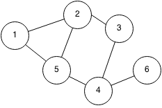
Figure 1: An Example Graph for Cycle Constraints.

For instance, consider the graph in Figure 1 and the cycle $\mathcal{C}=\{(1,2);(2,3);(3,4);(4,5);(5,1)\}$. If we consider paths starting from node $1$, we have $\mathcal{S}_{11}=\mathcal{S}_{12}=\mathcal{S}_{15}=\emptyset,~{}\mathcal{S}_{13}=\{2\},~{}\text{and }\mathcal{S}_{14}=\{5\}$. Therefore, $\mathcal{S}_{1}(\mathcal{C})=\{1,2,5\}$. If we take node $2$ to be the source, we have $\mathcal{S}_{22}=\mathcal{S}_{21}=\mathcal{S}_{25}=\mathcal{S}_{23}=\emptyset,~{}\text{and }\mathcal{S}_{24}=\{3\}$. This leads to $\mathcal{S}_{2}(\mathcal{C})=\{2,3\}$.

Theorem 3.

Given a cycle $\mathcal{C}$ and an arbitrary reference node $r$ in $\mathcal{C}$, Kirchhoff’s Voltage Law can be expressed as

$$\sum_{\begin{subarray}{c}(i,j)\in\mathcal{C}\end{subarray}}\frac{\left(\prod\limits_{(k,l)\in\mathcal{P}_{rj}}W_{kl}^{*}\right)\left(\prod\limits_{s\in\mathcal{S}_{r}(\mathcal{C})\setminus\mathcal{N}\left(\mathcal{P}_{rj}\right)}w_{s}\right)\left(W_{ij}-w_{j}\right)}{w_{j}}=0$$ (29)

Proof.

The proof uses the following two identities:

$$(V_{i}-V_{j})V_{j}^{*}=W_{ij}-w_{j}$$ (30)

$$\frac{1}{V_{j}^{*}}=\frac{V_{j}}{w_{j}}$$ (31)

$$\sum_{\begin{subarray}{c}(i,j)\in\mathcal{C}\end{subarray}}(V_{i}-V_{j})=0$$

$$\Updownarrow$$

$$\sum_{\begin{subarray}{c}(i,j)\in\mathcal{C}\end{subarray}}\frac{(V_{i}-V_{j})V_{j}^{*}}{V_{j}^{*}}=0$$

$$\Updownarrow\eqref{eq:id1}$$

$$\sum_{\begin{subarray}{c}(i,j)\in\mathcal{C}\end{subarray}}\frac{W_{ij}-w_{j}}{V_{j}^{*}}=0$$

$$\Updownarrow\eqref{eq:id2}$$

$$\sum_{\begin{subarray}{c}(i,j)\in\mathcal{C}\end{subarray}}\frac{V_{j}(W_{ij}-w_{j})}{w_{j}}=0$$

$$\Updownarrow$$

$$V_{r}^{*}\left(\prod\limits_{k\in\mathcal{S}_{r}(\mathcal{C})}V_{k}{V_{k}}^{*}\right)\sum_{\begin{subarray}{c}(i,j)\in\mathcal{C}\end{subarray}}\frac{V_{j}(W_{ij}-w_{j})}{w_{j}}=0$$

$$\Updownarrow$$

$$\sum_{\begin{subarray}{c}(i,j)\in\mathcal{C}\end{subarray}}\frac{V_{r}^{*}\left(\prod\limits_{k\in\mathcal{S}_{r}(\mathcal{C})}V_{k}{V_{k}}^{*}\right)V_{j}(W_{ij}-w_{j})}{w_{j}}=0$$

$$\Updownarrow\eqref{eq:lift1},\eqref{eq:lift}$$

$$\sum_{\begin{subarray}{c}(i,j)\in\mathcal{C}\end{subarray}}\frac{\left(\prod\limits_{(k,l)\in\mathcal{P}_{rj}}W_{kl}^{*}\right)\left(\prod\limits_{s\in\mathcal{S}_{r}(\mathcal{C})\setminus\mathcal{N}\left(\mathcal{P}_{rj}\right)}w_{s}\right)(W_{ij}-w_{j})}{w_{j}}=0.$$

∎

For illustration purposes, consider a three-bus cycle $\mathcal{C}=\{(1,2),(2,3),(3,1)\}$. It is easy to check that $\mathcal{P}_{11}=\emptyset$, $\mathcal{P}_{12}=\{(1,2)\}$, $\mathcal{P}_{13}=\{(1,3)\}$, leading to $\mathcal{S}_{ij}=\emptyset,~{}\forall(i,j)\in\mathcal{C}$, and $\mathcal{S}_{1}(\mathcal{C})=\{1\}$. Taking node $1$ to be the reference node and applying Theorem 3, we have,

$$\sum_{\begin{subarray}{c}(i,j)\in\mathcal{C}\end{subarray}}\frac{\left(\prod\limits_{(k,l)\in\mathcal{P}_{1j}}W_{kl}^{*}\right)\left(\prod\limits_{s\in\mathcal{S}_{1}(\mathcal{C})\setminus\mathcal{N}(\mathcal{P}_{1j})}w_{s}\right)(W_{ij}-w_{j})}{w_{j}}=0$$

$$\Downarrow$$

$$\frac{W_{12}^{*}(W_{12}-w_{2})}{w_{2}}+\frac{W_{13}^{*}(W_{23}-w_{3})}{w_{3}}+w_{1}\frac{W_{31}-w_{1}}{w_{1}}=0$$

$$\Downarrow$$

$$\frac{|W_{12}|^{2}-W_{12}^{*}w_{2}}{w_{2}}+\frac{W_{13}^{*}(W_{23}-w_{3})}{w_{3}}+W_{31}-w_{1}=0$$

$$\Downarrow$$

$$\frac{w_{1}w_{2}-W_{12}^{*}w_{2}}{w_{2}}+\frac{W_{13}^{*}(W_{23}-w_{3})}{w_{3}}+W_{31}-w_{1}=0$$

$$\Downarrow$$

$$w_{1}-W_{12}^{*}+\frac{W_{13}^{*}W_{23}}{w_{3}}-W_{13}^{*}+W_{31}-w_{1}=0$$

$$\Downarrow$$

$$W_{13}^{*}W_{23}=w_{3}W_{12}^{*}.$$

In real number representation, this is equivalent to

$$w^{R}_{31}w^{R}_{23}-w^{I}_{31}w^{I}_{23} =w_{3}w^{R}_{12},$$ (32)

$$w^{I}_{31}w^{R}_{23}+w^{R}_{31}w^{I}_{23} =-w_{3}w^{I}_{12}.$$ (33)

Note that one can generate another system of equations by setting the reference node to be $2$ before applying Theorem 3, which leads to

$$w^{R}_{31}w^{R}_{12}+w^{I}_{31}w^{I}_{12} =w_{1}w^{R}_{23},$$ (34)

$$w^{I}_{31}w^{R}_{12}-w^{R}_{31}w^{I}_{12} =-w_{1}w^{I}_{23}.$$ (35)

IV-B Linking the SDP Relaxation and Kirchhoff’s Voltage Law

Consider the $3\times 3$ matrix defined in (26), the determinant constraint is written,

$$det({W})\geq 0$$

$$\Updownarrow$$

$$-W_{12}\left(W_{12}^{*}W_{33}-W_{23}W_{13}^{*}\right)+W_{22}\left(W_{11}W_{33}-W_{13}W_{13}^{*}\right)$$

$$-W_{23}^{*}\left(W_{11}W_{23}-W_{13}W_{12}^{*}\right)\geq 0$$

$$\Updownarrow$$

$$-|W_{12}|^{2}W_{33}+W_{12}W_{23}W_{13}^{*}+W_{22}W_{11}W_{33}-|W_{13}|^{2}W_{22}$$

$$-|W_{23}|^{2}W_{11}+\left(W_{23}W_{13}^{*}W_{12}\right)^{*}\geq 0$$

$$\Updownarrow$$

$$2\mathcal{R}\left(W_{12}W_{23}W_{13}^{*}\right)+W_{11}W_{22}W_{33}$$

$$\geq|W_{12}|^{2}W_{33}+|W_{13}|^{2}W_{22}+|W_{23}|^{2}W_{11}$$

$$\Updownarrow$$

$$2\left(w_{12}^{R}\left(w_{23}^{R}w_{31}^{R}-w_{23}^{I}w_{31}^{I}\right)-w_{12}^{I}\left(w_{23}^{I}w_{31}^{R}+w_{23}^{R}w_{31}^{I}\right)\right)$$

$$\geq|W_{12}|^{2}W_{33}+|W_{13}|^{2}W_{22}+|W_{23}|^{2}W_{11}-W_{11}W_{22}W_{33}.$$

Now, observe that the linear combinations of the cycle constraints

$$w^{R}_{12}\eqref{eq:cycle_r}+w^{I}_{12}\eqref{eq:cycle_i}\text{ and }w^{R}_{23}\eqref{eq:cycle2_r}+w^{I}_{23}\eqref{eq:cycle2_i}$$

lead to

$$w_{12}^{R}\left(w_{23}^{R}w_{31}^{R}-w_{23}^{I}w_{31}^{I}\right)-w_{12}^{I}\left(w_{23}^{I}w_{31}^{R}+w_{23}^{R}w_{31}^{I}\right)=|W_{12}|^{2}W_{33}$$ (36)

$$w_{12}^{R}\left(w_{23}^{R}w_{31}^{R}-w_{23}^{I}w_{31}^{I}\right)-w_{12}^{I}\left(w_{23}^{I}w_{31}^{R}+w_{23}^{R}w_{31}^{I}\right)=|W_{23}|^{2}W_{11}$$ (37)

which represent the main components of the SDP determinant constraint presented previousely. Furthermore, based on (24), one has,

$$W_{11}W_{33}\geq|W_{13}|^{2}$$

$$\Updownarrow$$

$$W_{11}W_{22}W_{33}\geq W_{22}|W_{13}|^{2}$$ (38)

It is easy to show that (36) + (37) + (38) $\equiv$ (25). This establishes the fact that, for three-dimensional cycles, the SDP formulation captures a relaxed version of the cycle constraints (32)-(35) combined with the SOCP constraints (22).

V Numerical Experiments

This section presents a preliminary computational evaluation of the polynomial SDP cuts.

In the current experiments, only three-dimensional SDP cuts were generated. Implementation to handle higher dimension matrices is ongoing work.

The relaxations were compared on a subset of the NESTA v0.5.0 [10] benchmarks. NESTA is a comprehensive library including state-of-the-art AC-OPF transmission system test cases ranging from 3 to 9000 nodes and consist of 35 different networks under three modes: a typical operating condition (TYP), a congested operating condition (API), small angle difference condition (SAD) and radial configurations (RAD). In our preliminary experiments, we focus on small and medium size meshed instances of up to 300 nodes under typical operating conditions. Nonlinear models were solved using IPOPT 3.12 [7] with linear solver ma27 [11]. The SDP relaxation was executed on the state-of-the-art implementation [12] which already exploits the branch decomposition theorem [13]. The SDP solver SDPT3 4.0 [14] was used with the modifications suggested in [12]. Note that the phase angle bounds defined in Model 1 were also introduced in the SDP formulation. All instances were ran on a Dell PowerEdge R415 servers with Dual 2.8GHz AMD 6-Core Opteron 4184 CPUs and 64GB of memory.

IPOPT [7] is also used as a heuristic to find a feasible solution to the AC-OPF problem, providing an upper bound value on the optimal objective. We then measure the optimally gap between the heuristic and the relaxation using the formula

$$\frac{\text{Heuristic - Relaxation}}{\text{Heuristic}}$$

Table I and II present the results in terms of optimality gap and computational time, comparing the new polynomial SDP cut formulation (P-SDP) with the original SDP model and the standard SOCP relaxation respectively. Let us emphasize that we only generate 3-dimensional determinant cuts in these experiments and that the gap can be further reduced by generating cuts with higher dimensions. It is interesting to note that these 3-dimension cuts are already reducing the optimality gap from $2.04\%$ to $0.68\%$ on average, when compared to the SOCP relaxation. The gap reduction is substantial on case_30_ieee, dropping from $15.88\%$ to $0.06\%$. The computational time results are also very promising, the new formulation is on average one order of magnitude faster than the SDP solver approach.

TABLE I: Comparing SDP with P-SDP on TYP instances

	Opt. Gap (%)		Runtime (seconds)
Test Case	SDP	P-SDP	SDP	P-SDP
case3_lmbd	0.39	0.39	3.83	0.02
case4_gs	0.00	0.00	4.00	0.03
case5_pjm	5.22	5.22	4.43	0.05
case6_c	0.00	0.00	4.31	0.05
case6_ww	0.00	0.62	4.54	0.04
case9_wscc	0.00	0.00	3.95	0.20
case14_ieee	0.00	0.00	4.11	0.10
case24_ieee_rts	0.00	0.01	5.54	0.13
case29_edin	0.00	0.08	8.12	0.39
case30_as	0.00	0.00	5.84	0.16
case30_fsr	0.00	0.37	6.04	0.15
case30_ieee	0.00	0.06	5.56	0.26
case39_epri	0.01	0.05⋆	6.90	0.29
case57_ieee	0.00	0.06	8.08	0.49
case73_ieee_rts	0.00	0.03	8.83	0.67
case89_pegase	0.00	0.17	18.79	2.44
case118_ieee	0.06	1.51	12.77	1.32
case162_ieee_dtc	1.08	4.02	35.28	1.34
case189_edin	0.07	0.17	12.95	1.05
case300_ieee	0.08	0.93	27.70	2.66
Average	0.34	0.68	9.57	0.59

bold - the polynomial cuts match the SDP gap,
$\star$ - solver reported numerical accuracy warnings

TABLE II: Comparing P-SDP with SOCP on TYP instances

	Opt. Gap (%)		Runtime (seconds)
Test Case	SOCP	P-SDP	SOCP	P-SDP
nesta_case3_lmbd	1.32	0.39	0.09	0.02
case4_gs	0	0.00	0.04	0.03
case5_pjm	14.54	5.22	0.06	0.05
case6_c	0.3	0.00	0.14	0.05
case6_ww	0.63	0.62	0.10	0.04
case9_wscc	0	0.00	0.05	0.2
case14_ieee	0.11	0.00	0.07	0.1
case24_ieee_rts	0.01	0.01	0.08	0.13
case29_edin	0.12	0.08	0.18	0.39
case30_as	0.06	0.00	0.09	0.16
case30_fsr	0.39	0.37	0.08	0.15
case30_ieee	15.88	0.06	0.07	0.26
case39_epri	0.05	0.05⋆	0.15	0.29
case57_ieee	0.06	0.06	0.14	0.49
case73_ieee_rts	0.03	0.03	0.24	0.67
case89_pegase	0.17	0.17	0.34	2.44
case118_ieee	1.83	1.51	0.20	1.32
case162_ieee_dtc	4.03	4.02	0.30	1.34
case189_edin	0.21	0.17	0.37	1.05
case300_ieee	1.18	0.93	0.50	2.66
Average	2.04	0.68	0.16	0.59

bold - smaller optimality gap,
$\star$ - solver reported numerical accuracy warnings

VI Conclusion

The polynomial SDP cuts introduced in this paper have a great potential in increasing the scalability of semidefinite programming approaches to tackle complex optimisation problems in power systems. The computational time improvement can have a huge impact when the model includes discrete variables and branching becomes mandatory. The time reduction then becomes a factor of the number of nodes explored in the branch & bound tree.

Further implementation work is needed to automatically generate the SDP determinant cuts for matrices with dimensions higher than three. The key idea would be to generate the cuts lazily using a separation algorithm. Such an approach would start by solving the SOCP relaxation, identifying a submatrix violating the determinant constraint, and adding the corresponding cut to the model. The process is then iterated until the duality gap is small enough or the matrix is shown to be positive semidefinite.

References

- [1] R. Jabr, “Radial distribution load flow using conic programming,” Power Systems, IEEE Transactions on, vol. 21, no. 3, pp. 1458–1459, Aug 2006.
- [2] H. L. Hijazi, C. Coffrin, and P. Van Hentenryck, “Convex Quadratic Relaxations for Mixed-Integer Nonlinear Programs in Power Systems,” NICTA Technical Report, March 2014.
- [3] S. Sojoudi and J. Lavaei, “Physics of power networks makes hard optimization problems easy to solve,” in Power and Energy Society General Meeting, 2012 IEEE, July 2012, pp. 1–8.
- [4] J. E. PRUSSING, “The principal minor test for semidefinite matrices,” Journal of Guidance, Control, and Dynamics, vol. 9, no. 1, pp. 121–122, 2015/09/28 1986.
- [5] J. Lasserre, “On representations of the feasible set in convex optimization,” Optimization Letters, vol. 4, no. 1, pp. 1–5, 2010.
- [6] ——, “On convex optimization without convex representation,” Optimization Letters, vol. 5, no. 4, pp. 549–556, 2011.
- [7] A. Wächter and L. T. Biegler, “On the implementation of a primal-dual interior point filter line search algorithm for large-scale nonlinear programming,” Mathematical Programming, vol. 106, no. 1, 2006.
- [8] R. Madani, M. Ashraphijuo, and J. Lavaei, “Promises of conic relaxation for contingency-constrained optimal power flow problem,” Power Systems, IEEE Transactions on, vol. PP, no. 99, pp. 1–11, 2015.
- [9] B. Kocuk, S. S. Dey, and X. A. Sun, “Strong SOCP Relaxations for the Optimal Power Flow Problem,” ArXiv e-prints, Apr. 2015.
- [10] C. Coffrin, D. Gordon, and P. Scott, “NESTA, The Nicta Energy System Test Case Archive,” CoRR, vol. abs/1411.0359, 2014. [Online]. Available: http://arxiv.org/abs/1411.0359
- [11] R. C. U.K., “The hsl mathematical software library,” Published online at http://www.hsl.rl.ac.uk/, accessed: 30/10/2014.
- [12] J. Lavaei, “Opf solver,” Published online at http://www.ee.columbia.edu/~lavaei/Software.html, oct. 2014, accessed: 22/02/2015.
- [13] R. Madani, M. Ashraphijuo, and J. Lavaei, “Promises of conic relaxation for contingency-constrained optimal power flow problem,” Published online at http://www.ee.columbia.edu/~lavaei/SCOPF_2014.pdf, 2014, accessed: 22/02/2015.
- [14] K. C. Toh, M. Todd, and R. H. Ttnc, “Sdpt3 – a matlab software package for semidefinite programming,” Optimization Methods and Software, vol. 11, pp. 545–581, 1999.