Temporal Logic as Filtering

Abstract

We show that metric temporal logic (MTL) can be viewed as linear time-invariant filtering, by interpreting addition, multiplication, and their neutral elements, over the idempotent dioid ($\max$,$\min$,0,1). Moreover, by interpreting these operators over the field of reals (+,$\times$,0,1), one can associate various quantitative semantics to a metric-temporal-logic formula, depending on the filter’s kernel used: square, rounded-square, Gaussian, low-pass, band-pass, or high-pass. This remarkable connection between filtering and metric temporal logic allows us to freely navigate between the two, and to regard signal-feature detection as logical inference. To the best of our knowledge, this connection has not been established before. We prove that our qualitative, filtering semantics is identical to the classical MTL semantics. We also provide a quantitative semantics for MTL, which measures the normalized, maximum number of times a formula is satisfied within its associated kernel, by a given signal. We show that this semantics is sound, in the sense that, if its measure is 0, then the formula is not satisfied, and it is satisfied otherwise. We have implemented both of our semantics in Matlab, and illustrate their properties on various formulas and signals, by plotting their computed measures.

1 Introduction

Starting with natural sciences, such as, chemistry, physics, and mathematics, and ending with the applied sciences, such as, mechanical engineering, electrical engineering, and computer science, the process of filtering plays a central role. In each of the above-mentioned domains, it takes a signal $u$ as input, and it produces a signal $y$ as output, where the components of $u$ satisfying some given property are removed.

For example, in chemistry, a filter $f$ may remove particular molecules from a given solution. In optics (physics) and electrical engineering, $f$ may remove particular frequencies of $u$, as in a low-pass, high-pass or band-pass filter. Finally, in computer science (eg. in functional programming), $f$ may remove the elements in a list that satisfy a predicate $p$.

If the relation between $u$ and $y$ is linear, that is, if $f(u)$ is a linear function, the filter is called linear, otherwise it is called nonlinear. Moreover, if the operation of $f$ depends only on the values of $u$ and not on time, the filter is called time invariant. The most commonly used filters, in all of the above areas, are the linear, time-invariant (LTI) filters.

Intuitively, an LTI filter operates by sweeping a kernel distribution $k(s)$ over the entire domain of the lagged input signal $u(t{-}s)$, performing for every $s$ the multiplication $u(t{-}s)k(s)$, and than summing up (or integrating) the results, in order to obtain the value of the output signal $y(t)$ at time $t$. One says that $y\,{=}\,u{*}k\,{=}\,k{*}u$ is the convolution of $u$ and $k$.

If one interprets $(+,\times,0,1)$ over the field of reals, then filtering a discrete- or continuous-time {0,1}-valued signal $u$ results in a signal $y$ ranging over the reals. One can speak in this case about a quantitative semantics of the LTI filter:

$$y(n)\,{=}\sum\limits_{i\,{=}\,0}^{\infty}u(n-i)k(i),\quad y(t)\,{=}\int\limits_{0}^{\infty}u(t-s)k(s)\,ds.$$ (1)

An important aspect of an LTI filter $f$ is that, the kernel $k$ is the response $f(\delta(s))$ of the filter to an impulse $\delta$ placed at the origin. In discrete time, $\delta$ is the Kronecker function, while in continuous time, $\delta$ is the Dirac distribution.

If one interprets $(+,\times,0,1)$ over the ($\max$,$\min$,0,1) idempotent dioid [15], then filtering a discrete- or continuous-time {0,1}-valued signal $u$, results in a {0,1}-valued signal $y$. In this case, one can speak about a qualitative semantics of the LTI filter. The filter has in this case the following form:

$$y(t)\,{=}\sup\limits_{s\,{=}\,0}^{\infty}\min(u(t-s),\,k(s)).$$ (2)

This qualitative semantics can be readily mapped to either linear temporal logic (LTL), or to metric temporal logic (MTL), by using discrete time for LTL, discrete or continuous time for MTL, and choosing a rectangular window distribution $k$. In particular, (2) will represent the finally operator. The other LTL/MTL operators can also be defined, either by duality, or by choosing appropriate kernels $k$.

To the best of our knowledge, this remarkable correspondence between LTI filters and MTL has not been established before. This correspondence allows us to freely navigate between logic and signal processing, and to understand signal analysis, such as, feature detection, as a logical inference. It also allows us to equip MTL with various quantitative semantics, depending on the LTI-filter-kernel $k$ used: From square, to rounded, or to even a Gaussian windows, or from low-pass, to band-pass, or to even high-pass-filter kernel.

We prove that our qualitative, LTI-filtering semantics is identical to the classical MTL semantics. We also provide:

A quantitative semantics for MTL, which measures the normalized, maximum number of times a formula is satisfied within its associated kernel, with respect to a given signal.

We show that this quantitative semantics is sound, in the sense that, if its measure is 0, then the formula is not satisfied, and it is satisfied otherwise. We implemented both of our semantics in Matlab, and illustrate their properties on various formulas and signals by plotting their measures.

It is important to note that an LTI filter is called causal if the value of $u$ is known for the entire kernel $k$ at the time the multiplication is performed, and otherwise not-causal. This can be easily accomplished for signals with bounded domain. This restriction corresponds to bounded MTL, too. In the rest of the paper we will stick to this restriction.

The rest of the paper is organized as follows. In Section 2 we discuss related work. In Section 3 we revise MTL, and in Section 4 we revise LTI filters. In Section 5 we show that MTL semantics corresponds to a qualitative semantics in terms of LTI filters, and then also provide associated quantitative semantics, depending on the chosen kernel. Finally in Section 6 we draw conclusions and discuss future work.

2 Related Work

Linear temporal logic (LTL)[19], and metric temporal logic (MTL)[16], have proven to be concise and elegant formalisms for rigorously specifying a required temporal behaviour, for a system under investigation. While in LTL real time is not of concern (one speaks about logical time), in MTL all the logical formulas are qualified with a time interval (window), during which the system has to satisfy the corresponding formula. Moreover, while in LTL time is discrete, in MTL time can be either discrete or continuous. In fact, by restricting the windows in MTL to $[0,\infty]$, or the length of the signal, one can obtain LTL or bounded LTL, respectively.

The classical semantics for LTL or MTL is qualitative, that is, it provides a true or false answer, to whether a signal satisfies, or violates, a given LTL or MTL formula. Moreover, the signals themselves, are Boolean, too. With the increasing importance of analog- or even mixed digital-analog signals, this classical semantics has been extended to account for real-time, real-valued signals. To this end, the set of atomic propositions has been extended to also include relational propositions of the form $p\,{>}\,\theta$, where $\theta$ is a constant value, representing a threshold. By negation and conjunction, one obtains all other relational variations.

When monitoring LTL or MTL properties over real-time, real-valued, possibly noisy signals, the classic, true or false interpretation, has the limitation that, a small perturbation (also called a jitter), in either the temporal- or in the value-domain, may affect the overall verdict. In the last decade, there has been a concerted effort, to provide alternative ways to interpret LTL or MTL, by proposing a so called quantitative, or metric semantics for an LTL or MTL specification. This is often referred to as a measure of the specification.

In [20], Rizk et. al propose a quantitative semantics for an LTL over the reals (LTL($\mathbb{R}$)) that computes, using a constraint solving algorithm, the domain, that is, all the time points in which the real variables occurring in a formula, make this formula true, for a signal under analysis.

In [14], Fainekos et al. introduce a notion of space robustness for MTL, with numeric predicates interpreted over real-valued behaviors. The space robustness measures the degree by which a continuous signal satisfies or violates the specification. The key idea consists in computing for each moment of time the distance $x_{p}(t)\,{-}\,\theta$, and in using min and max, to summarize these distances. Consequently, min and max replace the Boolean operators and, and or. The temporal operators globally and eventually, had to be replaced accordingly, with inf and sup. This quantitative interpretation of MTL over real-time, real-valued signals, has found a number of applications in the hybrid systems community, for both the identification of the uncertain parameters [4, 11, 12] in a system, and for the falsification analysis of a model [3].

In [13], Donzé et al. define a notion of time robustness for MTL interpreted over dense-real-time, real-valued signals. The time robustness of a propositional formula evaluated at time $t$ measures the distance between $t$ and the nearest instant $t^{\prime}$ in which the proposition switches its value. The other logical and temporal operators are computed using the same rules as in the space robustness. In contrast, as shown in Section 5, we provide within the same filtering framework, both a qualitative and a quantitative semantics for MTL interpreted over real-time, Boolean-valued signals. Moreover, our quantitative semantics is different from time robustness. The latter does not allow to integrate the truth value of the formulas over time, and hence reason about the satisfaction rate of a specification.

Other notions of robustness based on accumulation have been in part explored in the discrete time setting, motivated by the goal to equip formal verification and synthesis with quantitative objectives. For example, in [5], Boker et al. investigate the extension of LTL with prefix-accumulation, path-accumulation, average and infinite average assertions. However, the interpretation of this extended logic remains in the Boolean domain. Another related approach consists in extending temporal logics with discounting operators [9, 2] weighting the importance of the events according to how late they occur. In the context of real-time, the Duration Calculus (DC) [7] is an interval logic containing the special duration operator. This operator allows to integrate the truth values of state expressions over an interval of time. Recently, Akazaki et al. [1] extend MTL with average temporal operators that quantifies the average over time of the space and time robustness previously introduced. The aforementioned logics based on the idea of accumulation share a common aspect – they are all equipped with special syntactic constructs that allow to specify integration of values. This is in contrast to our work, in which we use convolution to provide the power of value accumulation directly to the semantics of MTL without the need to adapt its syntax. Finally, we also note that we are not aware of any previous studies that relate convolution and filtering to the specification formalisms described in this section.

Figure 1: Measuring the spiking rate of a neuron.

3 Metric Temporal Logic

Let $P\,{=}\,\{p_{1},\ldots,p_{n}\}$ be a set of atomic propositions. A signal $x\,{:}\,\mathbb{T}\,{\rightarrow}\,2^{P}$ over $P$ is a set-valued function, with time domain $\mathbb{T}$. In this paper, we only consider finite-length signals, that is, we restrict their domains to $\mathbb{T}\,{=}\,[0,T]$, for an arbitrary, finite value $T$. In other words, $\mathbb{T}$ is an interval which is either a subset of non-negative reals $\mathbb{R}_{\geq 0}$ or naturals $\mathbb{N}$. We denote by $x_{p}$ the projection of $x$ to the proposition $p$.

Metric Temporal Logic (MTL) [16] is a real-time extension of Linear Temporal Logic (LTL) [19]. We consider a bounded variant of MTL that contains both future and past temporal operators. Its principal modalities are timed until $\until_{I}$ and since $\since_{I}$, where $I$ is a non-empty interval.

We provide a generic definition of MTL which is consistent with both the dense and discrete time interpretation of signals. Formally, the syntax of MTL interpreted over such signals is defined by the following grammar:

$$\varphi:=p\mid\neg\varphi\mid\varphi_{1}\vee\varphi_{2}\mid\varphi_{1}U_{I}\varphi_{2}\mid\varphi_{1}S_{I}\varphi_{2},$$

where $p\,{\in}\,P$ and $I$ is a non-empty interval of the form $\langle{a,b}\rangle$, such that, the left boundary $\langle$ is either open ( or closed [, the right boundary $\rangle$ is either open ) or closed ], and the boundary values $a,b\in\mathbb{N}$ are natural numbers with $0\,{\leq}\,a\,{\leq}\,b$.

The satisfaction of a given formula $\varphi$ with respect to a signal $x$ at time point $i$ is a relation denoted by $(x,i)\models\varphi$ and defined inductively as follows:

$$(x,i)\models p \iff x_{p}[i]=1$$

$$(x,i)\models\neg\varphi \iff (x,i)\not\models\varphi$$

$$(x,i)\models\varphi\vee\psi \iff (x,i)\models\varphi\;\textrm{or}\;(x,i)\models\psi$$

$$(x,i)\models\varphi\until_{I}\psi \iff \exists j\in(i+I)\cap\mathbb{T}\;\textrm{:}\;(x,j)\models\psi\;$$

$$\textrm{and}\;\forall k\in(i,\,j),\ (x,k)\models\varphi$$

$$(x,i)\models\varphi\since_{I}\psi \iff \exists j\in(i-I)\cap\mathbb{T}\;\textrm{:}\;(x,j)\models\psi\;$$

$$\textrm{and}\;\forall k\in(j,\,i),\ (x,k)\models\varphi.$$

From the basic definition of MTL, we can derive other standard Boolean and temporal operators as follows:

$$\begin{array}[]{l}\top=p\vee\neg p,\quad\bot=\neg\top,\quad\varphi\wedge\psi=\neg(\neg\varphi\vee\neg\psi),\\[2.84526pt] \F_{I}\varphi=\top\until_{I}\varphi,\quad\G_{I}\varphi=\neg\F_{I}\neg\varphi,\\[2.84526pt] \opP_{I}\varphi=\top\since_{I}\varphi,\quad\opH_{I}\varphi=\neg\opP_{I}\neg\varphi.\\[2.84526pt] \end{array}$$

The Finally $\F_{I}$, Globally $\G_{I}$, Once $\opP_{I}$ and Historically $\opH_{I}$ also admit a natural direct definition of their semantics:

$$\begin{array}[]{lcl}(x,i)\models\F_{I}\varphi&\iff&\exists j\in(i+I)\cap\mathbb{T}\;\textrm{:}\;(x,j)\models\varphi\\[2.84526pt] (x,i)\models\G_{I}\varphi&\iff&\forall j\in(i+I)\cap\mathbb{T},(x,j)\models\varphi\\[2.84526pt] (x,i)\models\opP_{I}\varphi&\iff&\exists j\in(i-I)\cap\mathbb{T}\;\textrm{:}\;(x,j)\models\varphi\\[2.84526pt] (x,i)\models\opH_{I}\varphi&\iff&\forall j\in(i-I)\cap\mathbb{T},(x,j)\models\varphi.\\ \end{array}$$

4 Linear Time-Invariant Filters

One of the most fundamental operations in signal processing is linear filtering, that is, the convolution of a signal with an appropriately chosen kernel or window. From audio, to image, and to video processing, linear filtering is used to either transform a signal in an appropriate way (eg. blur, sharpen) or to detect its features (eg. edges, patterns).

In order to understand linear filtering, it is instructive to describe it first in terms of the most fundamental windowing primitives: the Kronecker $\delta$ function, for the discrete-time case, and the Dirac $\delta$ distribution, for the continuous-time case. This distribution is defined as follows:

$$\delta(n)\,{=}\,\begin{cases}\infty,&\mbox{if }n=0\\ 0,&\mbox{otherwise},\end{cases}\qquad\int\limits_{-\infty}^{+\infty}\delta(s)\,ds\,{=}\,1.$$ (3)

It is interesting to note, that Kronecker $\delta$ is a function, whereas Dirac $\delta$ is not, that is, it makes sense only within an integral. Starting with Cauchy and up to Dirac, it took a long time to properly define this distribution  [10, 6].

The main motivation for developing the impulse windowing primitive, was the ability to extract the instantaneous action of a function at a particular moment of time. For example, the impulse provided by a baseball bat when hitting the ball. This fundamental ability, allows to describe any discrete (or continuous) signal $x$ as an infinite summation (or integral):

$$x(n)\,{=}\sum\limits_{i\,{=}\,-\infty}^{\infty}x(n{-}i)\delta(i),\quad x(t)\,{=}\int\limits_{-\infty}^{+\infty}x(t{-}s)\delta(s)\,ds.$$ (4)

This infinite sum (or integral) is denoted as $x\,{*}\,\delta$ and it is called the convolution of $x$ and $\delta$. Convolution is commutative, that is, $x{*}y\,{=}\,y{*}x$. Since $x\,{=}\,x{*}\delta$, convoluting $x$ with $\delta$ is an identity transformation. Its main appeal, is that it allows to express any linear, time-invariant (LTI) function $f$, as the convolution of its response $y$ to an impulse $\delta$ at the origin, with its (lagged) input $u$. For the discrete-time case (the continuous-time case is analogue), one can write:

$$f(\sum\limits_{i\,{=}\,-\infty}^{\infty}u(n{-}i)\delta(i))\,{=}\,\sum\limits_{i\,{=}\,-\infty}^{\infty}u(n{-}i)f(\delta(i)),$$ (5)

where $y(i)\,{=}\,f(\delta(i))$ is the response of $f$ to $\delta$ at time zero. This response can be seen as the filtering kernel, and therefore $f$, as a linear, time-invariant filter. The popularity of such filters stems from the fact that the response of $f$ to an impulses $\delta$ at the origin is easy to determine experimentally.

Figure 2: Windowing function types

In order to motivate the use of various kernels (windows), and to establish a link between LTI-filtering and the semantics of MTL’s finally operator, we borrow an example from [8]: measuring the firing rate of a spiking neuron.

If one ignores the duration and the pulse-like shape of a spike (also called an action potential), a spike sequence $\rho$ can be simply characterized as a sum of Dirac distributions:

$$\rho(t)\,{=}\,\sum\limits_{i\,{=}\,0}^{n}\delta(t{-}t_{i}),\qquad\quad r\,{=}\,\frac{1}{T}\int\limits_{0}^{T}\rho(s)\,ds,$$ (6)

where $t_{i}$ is the time where the neuron generates a spike. The normalized integral $r$ of $\rho(t)$ over an interval [0,T], is called the spike-count rate for that interval.

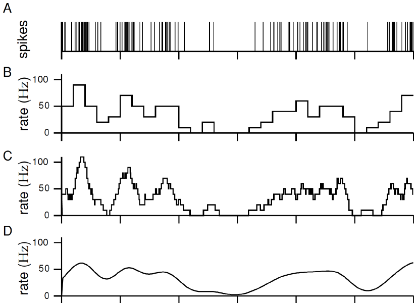
Now suppose one would like to approximate the spike rate of a neuron from an experimentally-obtained spike train. For example, Figure 1(A) shows the spike train obtained from a monkey’s inferotemporal-cortex neuron, while watching a movie. There are various ways to computing this rate.

A very simple-minded way is to divide the signal’s time domain in a set of disjoint bins, say of length $\Delta{t}$, count the number of spikes in each bin, and divide by $\Delta{t}$. For example, Figure 1(B) shows this approach, for $\Delta{t}\,{=}\,100$ms. The result is a discrete (in multiples of $1/\Delta{t}$), piecewise constant, function. Decreasing $\Delta{t}$ increases the temporal resolution, at the expense of the rate resolution. Moreover, the bin placement has an impact on the computed rates, too.

One can avoid an arbitrary bin-placement, by taking only one bin (or window) of duration $\Delta{t}$, slide it along the spike train, and then counting for each position $t$, the number of spikes within the bin. This approach is shown in Figure 1(C), where the window size is $\Delta{t}\,{=}\,100$ms. A centered discrete-time window can be defined as follows:

$$w_{\Delta{t}}(n)\,{=}\,\frac{1}{\Delta{t}}\sum\limits_{i\,{=}\,-\Delta{t}/2}^{+\Delta{t}/2}\delta(n{-}i).$$ (7)

A centered continuous-time window of size $\Delta{t}$ can be defined as follows (this would work in discrete-time, too):

$$w_{\Delta{t}}(t)\,{=}\,\begin{cases}1/\Delta{t},&\mbox{if }-\Delta{t}/2\,{\leq}\,t\,{\leq}\,\Delta{t}/2\\ 0,&\mbox{otherwise}.\end{cases}$$ (8)

Figure 3: Rectangular windows $w^{+}_{[1,4]}[t]$ and $w^{-}_{[1,4]}[t]$

The bin sliding along the spike train, the counting, and the normalization with $\Delta{t}$, can be succinctly expressed in terms of convolution, either in discrete or continuous time:

$$r(n)\,{=}\sum\limits_{i\,{=}\,0}^{T}\rho(i)w_{\Delta{t}}(n{-}i),\quad r(t)\,{=}\int\limits_{0}^{T}\rho(s)w_{\Delta{t}}(t{-}s)\,ds,$$ (9)

where $[0,T]$ is the domain of the spike train $\rho(t)$. If $\rho(t)$ is defined to be 0 outside $[0,T]$ one can take the sum (or the integral) over $[-\infty,+\infty]$. The convolution equation defines a discrete (and continuous) linear filter with kernel $w_{\Delta{t}}$. Note that the rates $r(t)$ at times less than one bin apart are correlated, because they involve common spikes. Moreover, the discontinuous nature of $r(t)$ is caused by the discontinuous nature of the window $w_{\Delta{t}}$ at its borders.

One can smoothen $r(t)$ and reduce the correlation between bins, by using a Gaussian window $N(0,\sigma)$ with $\sigma\,{=}\,100$ms, as shown in Figure 1(D). A Gaussian is defined as follows:

$$N(\mu,\sigma)(t)\,{=}\,\frac{1}{\sigma\sqrt{2\pi}}e^{-\frac{(t-\mu)^{2}}{2\sigma^{2}}}.$$ (10)

In fact, one could use any windowing function, as long as the area below the window (the integral) is one.

The spike train $\rho(t)$ discussed above could as well represent the truth-values of a discrete-time MTL signal $x$. Alternatively, connecting equal, successive values in $\rho(t)$, would result in the truth-values of a continuous-time MTL signal $x$. Hence, the LTI-filters above can be understood as a quantitative semantics for the MTL operators finally and once interpreted over $x$: The percentage of satisfaction of $x$ within the associated window. The size and the shape of the windows allow (as shown in the next section) to introduce a temporal jitter with respect to a satisfaction. Moreover, considering only square windows, and interpreting $(+,\times,0,1)$ over the idempotent dioid $(\max,\,\min,\,0,\,1)$ gives a logical, qualitative semantics to the LTI-filter as the classic finally operator.

5 MTL as LTI-Filtering

Figure 4: Qualitative discrete-time semantics.

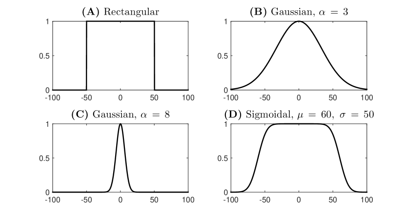
As it has already been mentioned before, all LTI-filters are characterized by the particular type of the kernel (window). Although there are a lot of such kernels, the main idea is the same: a kernel function should have a bounded support, that is, a bounded domain where the function is not zero.

General definitions allow such kernels to go sufficiently rapid towards zero. The simplest finite support window is when the function is constant inside of some interval, and zero elsewhere. This function is called a rectangular window or “Boxcar” (see Figure 2). A smooth Gaussian window is the second type of a window, because it extends to infinity. So it should be truncated at the ends of the window. The main advantage of such a function is its smooth nature.

Let us start with a rectangular window definition: for a given continuous-time MTL formula with constrained time interval $I\,{=}\,\langle{a},b\rangle$, a rectangular window function $w_{I}(t):\mathbb{R}\rightarrow[0,1]$ is constructed as follows:

$$w^{+}_{I}(t)\,{=}\,\begin{cases}\frac{1}{|I|},&\mbox{if }t\in\tilde{I}\\ 0,&\mbox{if }t\not\in\tilde{I},\end{cases}\quad w^{-}_{I}(t)\,{=}\,\begin{cases}\frac{1}{|I|},&\mbox{if }t\in I\\ 0,&\mbox{if }t\not\in I,\end{cases}$$ (11)

where $\tilde{I}\,{=}\,\langle{}{-}b,{-a}\rangle{}$ is used for the future MTL operators $\F_{I}$ or $\G_{I}$ and $I\,{=}\,\langle{}a,b\rangle{}$ for the past MTL operators $\opP_{I}$ or $\opH_{I}$. If $I\,{=}\,[a,a]$ is singular, then $w_{[a,a]}$ is defined as the Dirac-$\delta$ distribution. We will denote this window by $w_{\{a\}}$.

For discrete-time, open intervals can always be replaced with closed intervals. Hence we restrict $I$ to closed intervals, only. In this case, we define $w_{I}$ in terms of Kronecker-$\delta$, as follows:

$$w^{+}_{I}[t]\,{=}\,\frac{1}{|I|}\sum\limits_{i\,{\in}\,I}\delta(t+i),\quad w^{-}_{I}[t]\,{=}\,\frac{1}{|I|}\sum\limits_{i\,{\in}\,I}\delta(t-i),\\$$ (12)

where the ${+}$ and the ${-}$ superscripts correspond to the future and past MTL operators, respectively.

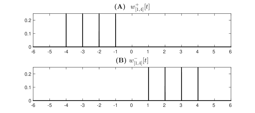
Note that for past MTL operators one needs to delay the kernel, so the sign is negative, and for future MTL operators one has to rush the kernel, so the sign is positive. For instance, consider the discrete-time MTL formulas $\F_{[1,4]}\,p$ and $\opP_{[1,4]}\,p$. The windows used by these formulas:

$$w^{+}_{[1,4]}[t]\,=\,\frac{1}{4}\sum\limits_{i=1}^{4}\delta(t+i),\quad w^{-}_{[1,4]}[t]\,=\,\frac{1}{4}\sum\limits_{i=1}^{4}\delta(t-i),$$ (13)

are shown graphically in Figure 3(A) and (B), respectively.

5.1 Qualitative Semantics

Figure 5: Continuous-time semantics for $p\since_{[2,4]}{q}$

In this section, we show that all temporal operators of MTL can be defined in terms of LTI-filtering. For this purpose, we interpret addition, multiplication, and their associated neutral elements over $(\{0,1\},\max,\min,0,1)$ the max-min idempotent dioid with value domain {0,1}. In this dioid one can define the complement $\neg{v}$ of a value $v$ as $1{-}v$. Moreover, the normalization factor in the definition of the window function $w_{I}(t)$ should be omitted in order to preserve Boolean values.

5.1.1 Discrete-time semantics

In the discrete-time domain, any signal is bounded (remember that we only consider bounded MTL), and therefore all the intervals of the MTL operators are bounded, too. As a consequence, the number of discrete points in each interval is finite, and we can extend the binary $\max$ operator to an n-ary max operator, which we can use for the convolution integral. Thus, the discrete-time semantics of MTL can be formulated as below:

$$(x,i)\models p \iff x_{p}[i]$$

$$(x,i)\models\neg\varphi \iff 1-(\,(x,i)\models\varphi\,)$$

$$(x,i)\models\varphi\vee\psi \iff \max\left((x,i)\models\varphi,\,(x,i)\models\psi\right)$$

$$(x,i)\models{\F}_{I}\varphi \iff \max_{j\,\in\,\mathbb{T}}\min\left((x,j)\models\varphi,\,w^{+}_{I}[i\,{-}\,j]\right)$$

$$(x,i)\models{\G}_{I}\varphi \iff 1-(\,(x,i)\models{\F}_{I}\neg\varphi\,)$$

$$(x,i)\models{\opP}_{I}\varphi \iff \max_{j\,\in\,\mathbb{T}}\min\left((x,j)\models\varphi,\,w^{-}_{I}[i\,{-}\,j]\right)$$

$$(x,i)\models{\opH}_{I}\varphi \iff 1-(\,(x,i)\models{\opP}_{I}\neg\varphi\,)$$

$$(x,i)\models\varphi\until_{I}\psi \iff \max_{j\,\in\,I}\min\Big{(}(x,i)\models{\G}_{[1,j-1]}\varphi,\,$$

$$(x,i)\models{\F}_{\{j\}}\psi\Big{)}$$

$$(x,i)\models\varphi\since_{I}\psi \iff \max_{j\,\in\,I}\min\Big{(}(x,i)\models{\opH}_{[1,j{-}1]}\varphi,\,$$

$$(x,i)\models{\opP}_{\{j\}}\psi\Big{)}.$$

In fact, we can define the entire semantics of MTL in terms of LTI-filtering, by using the Kronecker-$\delta$ kernel:

$$(x,i)\models p \iff \max_{j\,\in\,\mathbb{T}}\min\left(x_{p}[j],\,\delta(i-j)\right)$$

$$(x,i)\models\neg\varphi \iff \max_{j\,\in\,\mathbb{T}}\min\left(1-((x,j)\models\varphi),\delta(i-j)\right)$$

$$(x,i)\models\varphi\vee\psi \iff \max_{j\,\in\,\mathbb{T}}\min\Big{(}\max\big{(}$$

$$(x,j)\models\varphi,\,(x,j)\models\psi\big{)},\,\delta(i-j)\Big{)}.$$

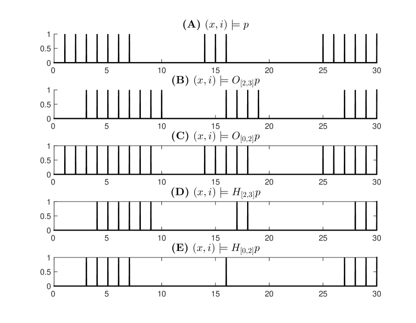
In order, to illustrate the qualitative, discrete-time semantics for various temporal operators, consider the example shown in Figure 4. In Figure 4(A) we show the values $x_{p}$ of discrete-time signal $x$, for which it satisfies proposition $p$. This signal is defined over the interval $[0,30]$, with $\Delta{t}\,{=}\,1$. In other words, the domain of $x$ is $\{0,1,\ldots,30\}$.

In order to interpret the MTL operators $\opP$ and $\opH$ over $x$, we use two indexing windows $I$, for both: The first is $I=[2,3]$, and the second is $I=[0,2]$. To simplify the caption in the Matlab figures, we use the textual representation of the temporal operators: F (finally) for $\F$, G (globally) for $\G$, O (once) for $\opP$, and H (historically) for $\opH$.

The satisfaction of the MTL formulas $\opP_{[2,3]}p$ and $\opP_{[0,2]}p$ for the signal $x_{p}$ are shown in Figure 4(B-C). Similarly, the satisfaction of $\opH_{[2,3]}p$ and $\opH_{[0,2]}p$ for the signal $x_{p}$ are shown in Figure 4(D-E). The dependence on the length of the interval $I$ is precise: Increasing the length, increases the number of points where the operator $\opP_{I}p$ is satisfied and $\opH_{I}p$ is not. Moreover, the shift of the interval’s beginning point leads to the same shift of the output signal.

For the qualitative, discrete-time semantics of an MTL formula $\varphi$ with respect to a signal $x$, it is straight forward to show, that the semantics is sound, in the sense that, if it produces the value 0, then the formula is not satisfied in the classical semantics, and if it produces 1 then it is satisfied. Let us index satisfaction with $C$ as classic semantics, and with $L$ as LTI-filtering semantics in the following theorem.

Theorem 1 (Soundness).

For an MTL formula $\varphi$ and a discrete-time signal $x$, it holds that $x$ satisfies $\varphi$ in the LTI-filtering interpretation, if and only if, it satisfies $\varphi$ in the classic interpretation. More formally one can write:

$$(x,i)\models_{L}\varphi \iff(x,i)\models_{C}\varphi.$$

Proof.

(Sketch) First, observe that the Boolean operators are interpreted the same way, as the max-min dioid provides a logical interpretation for the set {0,1}: the truth tables for conjunction and $\min$, disjunction and $\max$, and negation and complement, are all the same, respectively. Second, the existential quantifier in the classic interpretation, corresponds to max in the max-min dioid, which leads to the same interpretation for $\F_{I}$ and $\opP_{I}$. Through the properties of negation, we immediately establish the same interpretation for $\G_{I}$ and $\opH_{I}$. Finally, the definition of $\until_{I}$ and $\since_{I}$ can be written solely in terms of the previous temporal operators, as we did in the LTI-filter semantics. ∎

Figure 6: Qualitative continuous-time semantics.

5.1.2 Continuous-time semantics

Figure 7: Soundness of discrete-time semantics.

In the continuous-time semantics, each bounded interval is going to have an infinite number of points, except for the singular intervals, which contain only a single point. As a consequence, we have to interpret the integral in this case, as the supremum operator, which is the proper extension of $\max$ over infinite domains.

$$(x,i)\models p \iff x_{p}(i)$$

$$(x,i)\models\neg\varphi \iff 1-(\,(x,i)\models\varphi\,)$$

$$(x,i)\models\varphi\vee\psi \iff \max\left((x,i)\models\varphi,\,(x,i)\models\psi\right)$$

$$(x,i)\models{\F}_{I}\varphi \iff \sup_{j\,\in\,\mathbb{T}}\min\left((x,j)\models\varphi,\,w^{+}_{I}(i\,{-}\,j)\right)$$

$$(x,i)\models{\G}_{I}\varphi \iff 1-(\,(x,i)\models{\F}_{I}\neg\varphi\,)$$

$$(x,i)\models{\opP}_{I}\varphi \iff \sup_{j\,\in\,\mathbb{T}}\min\left((x,j)\models\varphi,\,w^{-}_{I}(i\,{-}\,j)\right)$$

$$(x,i)\models{\opH}_{I}\varphi \iff 1-(\,(x,i)\models{\opP}_{I}\neg\varphi\,)$$

$$(x,i)\models\varphi\until_{I}\psi \iff \sup_{j\,\in\,I}\min\Big{(}(x,i)\models{\G}_{(0,j)}\varphi,\,$$

$$(x,i)\models{\F}_{\{j\}}\psi\Big{)}$$

$$(x,i)\models\varphi\since_{I}\psi \iff \sup_{j\,\in\,I}\min\Big{(}(x,i)\models{\opH}_{(0,j)}\varphi,\,$$

$$(x,i)\models{\opP}_{\{j\}}\psi\Big{)}.$$

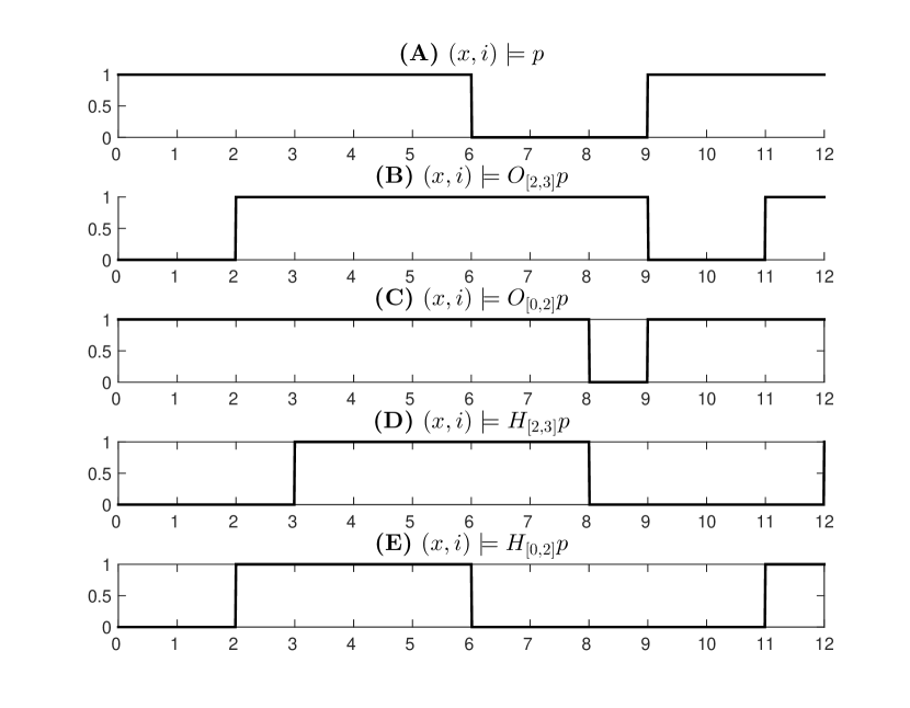
In order to illustrate the qualitative, continuous-time semantics for various temporal operators, consider the example shown in Figure 6. In Figure 6(A) we show $x_{p}$, the value of continuous-time signal $x$, for which proposition $p$ is true. This signal is defined over the interval $[0,12]$. Every sub-interval in the plot is left-closed and right-open.

In order to interpret the MTL operators $\opP$ and $\opH$ over $x$, we use, the same indexing windows as before: First, $I=[2,3]$ and next, $I=[0,2]$. The satisfaction of the MTL formulas $\opP_{[2,3]}p$ and $\opP_{[0,2]}p$ for the signal $x$ are shown in Figure 6(B-C). Similarly, the satisfaction of $\opH_{[2,3]}p$ and $\opH_{[0,2]}p$ for the signal $x$ are shown in Figure 6(D-E).

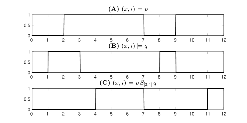
The qualitative, continuous-time semantics of the since operator $(x,i)\models p\since_{[2,4]}q$ is shown in Figure 5. The semantics of $(x,i)\models p$ (signal $x_{p}$) is shown in Figure 5(A) and the semantics of $(x,i)\models q$ (signal $x_{q}$) shown in Figure 5(B). Finally, the semantics of $(x,i)\models p\since_{[2,4]}q$ is shown in Figure 5(C). It should be emphasized that, the obtained qualitative semantics corresponds to a standard MTL semantics.

Theorem 2 (Soundness).

For an MTL formula $\varphi$ and a continuous-time signal $x$, it holds that $x$ satisfies $\varphi$ in the LTI-filtering interpretation, if and only if, it satisfies $\varphi$ in the classic interpretation. More formally one can write:

$$(x,i)\models_{L}\varphi \iff(x,i)\models_{C}\varphi.$$

Proof.

(Sketch) The proof is very similar to the one for the discrete-time, qualitative semantics. The only difference is that we work now with windows having dense (infinite) domain, and max have to be therefore extended to sup, the proper extension on such domains. ∎

5.2 Quantitative Semantics

Figure 8: Quantitative discrete-time semantics.

If we interpret addition, multiplication, and their associated neutral elements over $([0,1],+,\times,0,1)$, the field of reals restricted to the interval [0,1], we recover the standard definition of LTI-filtering. This definition allows us to associate a quantitative semantics to MTL temporal formulas.

This semantics measures the normalized, maximum number of times the formula is satisfied within its associated window. Since $\G_{I}$ and $\opH_{I}$ can be satisfied only once within $I$, the measure returns 1, in case of satisfaction, and 0, otherwise. However, $\F_{I}$ and $\opP_{I}$ are more interesting, as they may be satisfied several times in $I$. As in Section 5.1, we distinguish between discrete- and continuous-time semantics, and use summations and integrals, respectively.

Moreover, we give up the duality property between the $\G_{I}$ and $\F_{I}$ operators (same for past operators $\opH_{I}$ and $\opP_{I}$). In the rest of the paper we will stick to the positive normal form representation of an MTL formula, where negations may only occur in front of atomic propositions [18].

5.2.1 Discrete-time semantics

Assume we are given a discrete signal with $[0,T]$ duration interval. Then the quantitative semantics for MTL can be formulated as follows:

$$\val{x,p}[i] = x_{p}[i]$$

$$\val{x,\neg p}[i] = 1-\val{x,p}[i]$$

$$\val{x,\varphi\,{\vee}\,\psi}[i] = \max(\val{x,\varphi}[i],\ \val{x,\psi}[i])$$

$$\val{x,\varphi\,{\wedge}\,\psi}[i] = \min(\val{x,\varphi}[i],\ \val{x,\psi}[i])$$

$$\val{x,{\F}_{I}\varphi}[i] = \sum_{j\,{\in}\,\mathbb{T}}\ \val{x,\varphi}[j]\cdot w^{+}_{I}[i-j]$$

$$\val{x,{\opP}_{I}\varphi}[i] = \sum_{j\,{\in}\,\mathbb{T}}\ \val{x,\varphi}[j]\cdot w^{-}_{I}[i-j]$$

$$\val{x,{\G}_{I}\varphi}[i] = \min_{j\,{\in}\,i+I}\val{x,\varphi}[j]$$

$$\val{x,{\opH}_{I}\varphi}[i] = \min_{j\,{\in}\,i-I}\val{x,\varphi}[j]$$

$$\val{x,\varphi\until_{I}\psi}[i] = \frac{1}{|I|}\sum_{j\,{\in}\,I}\ \val{x,{\G}_{[1,j-1]}\varphi}[i]\cdot\val{x,{\F}_{\{j\}}\psi}[i]$$

$$\val{x,\varphi\since_{I}\psi}[i] = \frac{1}{|I|}\sum_{j\,{\in}\,I}\ \val{x,{\opH}_{[1,j-1]}\varphi}[i]\cdot\val{x,{\opP}_{\{j\}}\psi}[i],$$

where the window superscripts $+$ and $-$ correspond to the window direction, according to Equations (12).

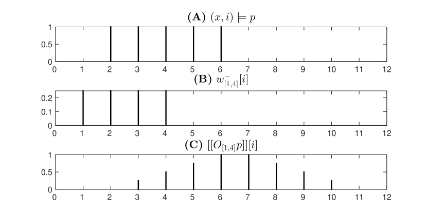
For example, consider the discrete-time signal $x$ over the interval $[0,12]$, with $\Delta{t}\,{=}\,1$, shown in Figure 8. Since it is discrete-time, its domain is $\{0,1,\ldots,12\}$. In order to interpret the MTL operator $\opP_{[1,4]}\,p$, we construct the rectangular windowing function $w^{-}_{[1,4]}[i]$ as shown at the beginning of Section 5. The representation of this window is shown in Figure  3(B). Since the MTL formula, is a past formula, the corresponding window is formally defined as follows:

Table 1: Quantitative semantics values

MTL Formula	Time point
	3	4	5	6	7	8	9	10
$\val{\opP_{[1,4]}p}$	$\frac{1}{4}$	$\frac{1}{2}$	$\frac{3}{4}$	1	1	$\frac{3}{4}$	$\frac{1}{2}$	$\frac{1}{4}$

$$w^{-}_{[1,4]}[i]\,{=}\,\frac{1}{4}\sum\limits_{j=1}^{4}\delta(i-j).$$ (14)

Now we are able to evaluate the quantitative semantics of signal $x$ with respect to the Once-formula given below:

$$\begin{array}[]{lcl}\val{\opP_{[1,4]}p}\left[i\right]=\sum\limits_{j=0}^{12}p[j]\cdot w^{-}_{[1,4]}[i-j].\end{array}$$

The quantitative-values of the result are given in a Table 1, and their graphical representation is shown in Figure 8.

For the quantitative, discrete-time semantics of an MTL formula $\varphi$ and signal $x$, it is straight forward to show, that the semantics is sound, in the sense that, it produces a measure greater than 0, if and only if, the formula is satisfied by the discrete-time qualitative semantics, and 0, otherwise.

Figure 9: Discrete quantitative semantics for $\since_{I}$.

Theorem 3 (Soundness).

For a positive normal form MTL formula $\varphi$ and a discrete-time signal $x$, it holds that $x$ satisfies $\varphi$, if and only if, its quantitative semantics is strictly greater than 0. It does not satisfy $\varphi$, if and only if, its quantitative semantics is 0:

$$(x,i)\models\varphi \iff\val{x,\varphi}[i]>0,$$

$$(x,i)\not\models\varphi \iff\val{x,\varphi}[i]=0.$$

Proof.

(Sketch) First, as shown in Theorem 1, the qualitative discrete-time semantics in terms of LTI-filtering over the idempotent dioid $(\max,\min,0,1)$, is the same as the classical MTL semantics. Second, the interpretation of Boolean MTL formulas $p$, $\neg p$, $\varphi\vee\psi$, and $\varphi\wedge\psi$ over $x$ is the same in both the qualitative and quantitative semantics. Third, the interpretation of the temporal MTL formulas $\G_{I}$ and $\opH_{I}$ over $x$ is also the same. Fourth, the interpretation of MTL formulas $\F_{I}$ and $\opP_{I}$ ensure that they are strictly positive only if they are satisfied by $x$ and 0, otherwise. Fifth, the interpretation of $\until_{I}$ and $\since_{I}$ are properly derived from $\G_{I}$ and $\F_{I}$, $\opH_{I}$ and $\opP_{I}$, respectively. ∎

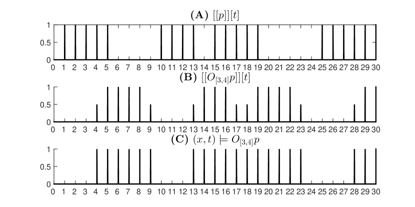
In order to illustrate the relation between the qualitative and the quantitative, discrete-time semantics, consider the example shown in Figure 7. In Figure 7(A) we show the signal $x_{p}$. This signal is defined over the set $\{0,\ldots,30\}$. In Figure 7(B) we illustrate the quantitative semantics of the formula $\opP_{[3,4]}p$ with respect to $x$, and in Figure 7(C) we show the qualitative semantics of the same formula with respect to $x$. As Figures 7(B-C) show, the two are in agreement, that is whenever the quantitative semantics is strictly greater than 0, the formula is satisfied, and whenever the quantitative semantics is 0, the formula is not satisfied.

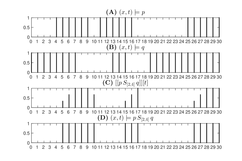
In Figure 9 we illustrate the interplay between the once and the historically operators as they occur in the definition of the since operator. Note that the outside sum also plays the role of an enclosing temporal operator. In Figure 9(A) and (B) we show the discrete-time signals $x_{p}$ and $x_{q}$, respectively. In Figure 9(C) we show the quantitative semantics of $p\since_{[2,4]}q$ with respect to $x_{p}$ and $x_{q}$. Finally in Figure 9(D), we show the qualitative semantics of the same formula with respect to $x_{p}$ and $x_{q}$. As one can see from Figure 9(C-D), the quantitative semantics is sound.

5.2.2 Continuous-time semantics

In the continuous-time semantics, we restrict ourselves to piecewise constant cadlag signals [17]. Such signals are right-continuous and have left limits everywhere. As a consequence, we do not consider signals that may have a distinct value in some isolated point. Since this property has to be preserved by temporal operators, we adopt the MTL fragment from [17], where temporal modalities are restricted to be closed intervals only. Assume we are given a signal $x$ with domain $[0,T)$. Then the quantitative semantics for MTL is defined as follows:

$$\val{x,p}(i) = x_{p}(i)$$

$$\val{x,\neg p}(i) = 1-\val{x,p}(i)$$

$$\val{x,\varphi\,{\vee}\,\psi}(i) = \max(\val{x,\varphi}(i),\ \val{x,\psi}(i))$$

$$\val{x,\varphi\,{\wedge}\,\psi}(i) = \min(\val{x,\varphi}(i),\ \val{x,\psi}(i))$$

$$\val{x,{\F}_{I}\varphi}(i) = \int\limits_{\mathbb{T}}\val{x,\varphi}(j)\cdot w^{+}_{I}(i{-}j)\ \mathrm{d}j$$

$$\val{x,{\opP}_{I}\varphi}(i) = \int\limits_{\mathbb{T}}\val{x,\varphi}(j)\cdot w^{-}_{I}(i{-}j)\ \mathrm{d}j$$

$$\val{x,{\G}_{I}\varphi}(i) = \inf_{j\,{\in}\,i+I}\val{x,\varphi}(j)$$

$$\val{x,{\opH}_{I}\varphi}(i) = \inf_{j\,{\in}\,i-I}\val{x,\varphi}(j)$$

$$\val{x,\varphi\until_{I}\psi}(i) = \frac{1}{|I|}\int\limits_{I}\val{x,{\G}_{(0,j)}\varphi}(i)\cdot\val{x,{\F}_{\{j\}}\psi}(i)\mathrm{d}j$$

$$\val{x,\varphi\since_{I}\psi}(i) = \frac{1}{|I|}\int\limits_{I}\val{x,{\opH}_{(0,j)}\varphi}(i)\cdot\val{x,{\opP}_{\{j\}}\psi}(i)\mathrm{d}j,$$

where the window superscripts $+$ and $-$ correspond to the direction of the window according to (12). As usual, the $\inf$ operation over an empty set is assumed to be 1.

Like in the discrete-time case, it is relatively straight-forward to show that the quantitative semantics of an MTL formula $\varphi$ with respect to a continuous-time signal $x$, is sound.

Figure 10: Soundness of continuous-time semantics.

Theorem 4 (Soundness).

Let $\varphi$ be a positive normal form MTL formula and $x$ be a continuous-time signal. Then the following properties hold:

$$\val{x,\varphi}(i)>0\quad \Longrightarrow\quad(x,i)\models\varphi,$$

$$(x,i)\not\models\varphi\quad \Longrightarrow\quad\val{x,\varphi}(i)=0.$$

Proof.

(Sketch) The proof goes along the same lines as the one for the discrete-time semantics, but with a set of complementary remarks. First, one has to observe that $\inf$ operator properly extends $\min$ and the integral properly extends the sum operator. Second, the Dirac-$\delta$ is the proper substitute of the Kronecker-$\delta$ within the integral. Third, if the MTL formula is valid only in a punctual interval within the given time constraints, it is not allowed to measure the normalized number of times the formula is satisfied within the window. In this case the quantitative measure is equal to zero and it is essential to drop the contrary claim. ∎

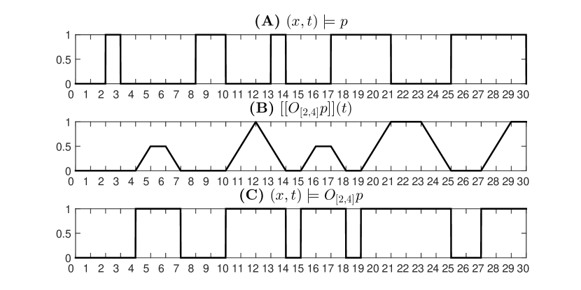
In order to illustrate the quantitative, continuous-time semantics for various temporal operators, and their relation to the qualitative, continuous-time semantics, consider the example shown in Figure 10. In Figure 10(A) we show the signal $x_{p}$. This signal is defined over the interval $[0,30)$. In Figure 10(B) we illustrate the quantitative semantics of the formula $\opP_{[2,4]}p$ with respect to $x$, and in Figure 10(C) we show the qualitative semantics of the same formula with respect to $x$. As Figures 10(B-C) show, the two are in agreement, that is whenever the quantitative semantics is strictly greater than 0, the formula is satisfied, and whenever formula is not satisfied, the quantitative semantics is 0.

Remark 1.

Note that for a singular interval $I=\{a\}$, the semantics of $\F_{I}\varphi$ or $\opP_{I}\varphi$ is not necessarily zero (although a point has zero area), because this interval is represented by the Dirac-$\delta$ distribution which is an “infinite” value at $a$:

$$\val{x,{\opP}_{\{a\}}\varphi}(t) =\int\limits_{0}^{T}\val{x,\varphi}(s)\cdot w^{-}_{\{a\}}(t-s)\ \mathrm{d}s=\val{x,\varphi}(t-a),$$

$$\val{x,{\F}_{\{a\}}\varphi}(t) =\int\limits_{0}^{T}\val{x,\varphi}(s)\cdot w^{+}_{\{a\}}(t-s)\ \mathrm{d}s=\val{x,\varphi}(t+a).$$

Moreover, the semantics of $\G_{I}$ and $\opH_{I}$ is also not zero, because of the infimum operator over a single point. As a consequence, we have that $\G_{I}\,{\equiv}\,\F_{I}$ and $\opH_{I}\,{\equiv}\,\opP_{I}$.

Figure 11: Smooth evaluation of $\val{\opP_{[1,6]}p}\left[t\right]$.

In order to illustrate the effect of applying various smooth kernels to a signal $x_{p}$, consider the example shown in Figure 11. In Figure 11(A) we show the signal $x_{p}$. In Figure 11(B) we illustrate the quantitative semantics with respect to a square kernel. In Figure 11(C) we show the same semantics with respect to a sigmoidal window. This automatically adds tolerance to a time-jitter at the boundaries of the kernel. Finally, in Figures 11(D-E) we show the result of applying Gaussian kernels, with reciprocal of standard deviation 8 and 3, respectively. Note how they influence the domain of satisfaction.

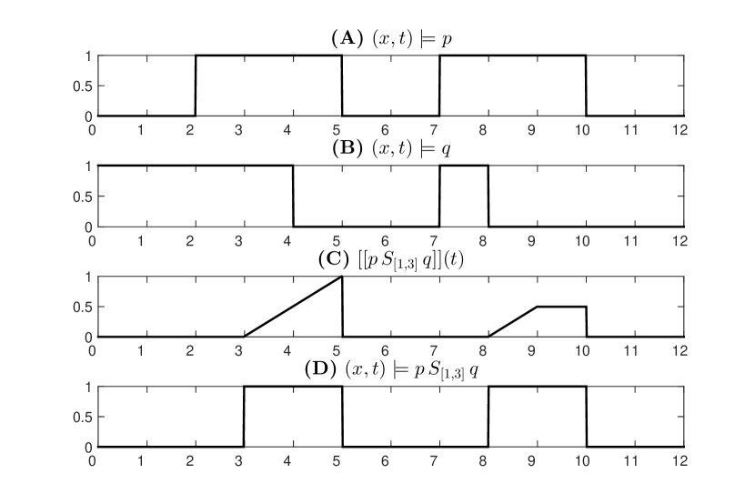
In Figure 12 we illustrate the since operator with respect to continuous-time signals $x_{p}$ and $x_{q}$. In Figures 12(A-B) we show these two signals. In Figure 12(C) we show the quantitative semantics of $p\since_{[1,3]}q$ with respect to $x_{p}$ and $x_{q}$. Finally in Figure 12(D), we show the qualitative semantics of the same formula with respect to $x_{p}$ and $x_{q}$. As one can see from Figures 12(C-D), the quantitative semantics is sound.

Figure 12: Cont. quantitative semantics for $\since_{I}$.

6 Conclusions

We have shown that linear, time-invariant (LTI) filtering corresponds to metric temporal logic (MTL) if addition and multiplication are interpreted as $\max$ and $\min$, and if true and false are interpreted as one and zero, respectively.

We have also provided a quantitative semantics to temporal MTL formula with respect to a discrete- or continuous-time signal, measuring the normalized, maximum number of times, the formula is satisfied within its associated window. This semantics is sound, in the sense that, if its measure is strictly greater than zero, then the formula is satisfied.

In future work we would like to explore alternative quantitative semantics for MTL, which are more informative, in case the MTL formula is not satisfied. We would also like to explore the logical meaning of other types of LTI-filter kernels, such as band-pass and high-pass. Moreover, we would like to investigate how the correspondence between MTL and LTI-filters can be exploited in order to build very efficient MTL monitors, using digital signal processors (DSPs). These are specialized microprocessors, optimized for filtering and compression operations in signal processing.

7 Acknowledgments

This work was partially supported by the Austrian FFG project HARMONIA (nr. 845631), the Doctoral Program Logical Methods in Computer Science funded by the Austrian FWF, the Austrian National Research Network (nr. S 11405-N23 and S 11412-N23) SHiNE funded by the Austrian Science Fund (FWF), the EU ICT COST Action IC1402 on Runtime Verification beyond Monitoring (ARVI), the US National-Science-Foundation Frontiers project CyberCardia, the MISTRAL project A-1341-RT-GP coordinated by the European Defence Agency (EDA) and funded by the Joint Investment Programme on Second Innovative Concepts and Emerging Technologies (JIP-ICET 2). The authors also would like to acknowledge César Sánchez from IMDEA Software Institute for helpful insight and comments that greatly improved the paper.

References

- [1] T. Akazaki and I. Hasuo. Time robustness in MTL and expressivity in hybrid system falsification. In Proc. of CAV 2015: the 27th International Conference on Computer Aided Verification, Part II, volume 9207 of LNCS, pages 356–374. Springer, 2015.
- [2] S. Almagor, U. Boker, and O. Kupferman. Discounting in LTL. In Proc. of TACAS 2015: the 20th International Conference on Tools and Algorithms for the Construction and Analysis of System, volume 8413 of LNCS, pages 424–439. Springer, 2014.
- [3] Y. S. R. Annapureddy, C. Liu, G. E. Fainekos, and S. Sankaranarayanan. S-taliro: A tool for temporal logic falsification for hybrid systems. In Proc. of TACAS 2011: the 17th International Conference on Tools and Algorithms for the Construction and Analysis of Systems, volume 6605 of LNCS, pages 254–257. Springer, 2011.
- [4] E. Bartocci, L. Bortolussi, L. Nenzi, and G. Sanguinetti. System design of stochastic models using robustness of temporal properties. Theor. Comput. Sci., 587:3–25, 2015.
- [5] U. Boker, K. Chatterjee, T. A. Henzinger, and O. Kupferman. Temporal specifications with accumulative values. ACM Trans. Comput. Log., 15(4):27:1–27:25, 2014.
- [6] A.-L. Cauchy. Th orie de la propagation des ondes la surface d’un fluide pesant d’une profondeur ind finie. Acad mie des sciences (France), 1815.
- [7] Z. Chaochen, C. A. R. Hoare, and A. P. Ravn. A calculus of durations. Inf. Process. Lett., 40(5):269–276, 1991.
- [8] P. Dayan and L. F. Abbott. Theoretical Neuroscience: Computational and Mathematical Modeling of Neural Systems. The MIT Press, 2001.
- [9] L. de Alfaro, M. Faella, T. A. Henzinger, R. Majumdar, and M. Stoelinga. Model checking discounted temporal properties. In Proc. of TACAS 2004: the 10th International Conference on Tools and Algorithms for the Construction and Analysis of Systems, volume 2988 of LNCS, pages 77–92. Springer, 2004.
- [10] P. Dirac. The Principles of Quantum Mechanics. Oxford University Press, 1930.
- [11] A. Donzé. Breach, a toolbox for verification and parameter synthesis of hybrid systems. In Proc. of CAV 2010: the 22nd International Conference on Computer Aided Verification, volume 6174 of LNCS, pages 167–170. Springer Berlin, 2010.
- [12] A. Donzé, G. Clermont, and C. J. Langmead. Parameter synthesis in nonlinear dynamical systems: Application to systems biology. Journal of Computational Biology, 17(3):325–336, 2010.
- [13] A. Donzé and O. Maler. Robust satisfaction of temporal logic over real-valued signals. In Proc. of FORMATS 2010: the 8th International Conference on Formal Modeling and Analysis of Timed Systems, volume 6246 of LNCS, pages 92–106. Springer, 2010.
- [14] G. E. Fainekos and G. J. Pappas. Robustness of temporal logic specifications for continuous-time signals. Theor. Comput. Sci., 410(42):4262–4291, 2009.
- [15] M. Gondran and M. Minoux. Graphs, Dioids and Semirings. Springer, 2008.
- [16] R. Koymans. Specifying real-time properties with metric temporal logic. Real-Time Systems, 2(4):255–299, 1990.
- [17] O. Maler, D. Nickovic, and A. Pnueli. From MITL to timed automata. In Formal Modeling and Analysis of Timed Systems, 4th International Conference, FORMATS 2006, Paris, France, September 25-27, 2006, Proceedings, pages 274–289, 2006.
- [18] J. Ouaknine and J. Worrell. On the decidability of metric temporal logic. In Logic in Computer Science, 2005. LICS 2005. Proceedings. 20th Annual IEEE Symposium on, pages 188–197. IEEE, 2005.
- [19] A. Pnueli. The temporal logic of programs. In 18th Annual Symposium on Foundations of Computer Science, Providence, Rhode Island, USA, 31 October - 1 November 1977, pages 46–57, 1977.
- [20] A. Rizk, G. Batt, F. Fages, and S. Soliman. Continuous valuations of temporal logic specifications with applications to parameter optimization and robustness measures. Theoretical Computer Science, 412(26):2827–2839, 2011.