The fundamental plane of star formation in galaxies revealed by the EAGLE hydrodynamical simulations

Abstract

We investigate correlations between different physical properties of star-forming galaxies in the “Evolution and Assembly of GaLaxies and their Environments” (eagle) cosmological hydrodynamical simulation suite over the redshift range $0\leq z\leq 4.5$. A principal component analysis reveals that neutral gas fraction ($f_{\rm gas,neutral}$), stellar mass ($M_{\rm stellar}$) and star formation rate (SFR) account for most of the variance seen in the population, with galaxies tracing a two-dimensional, nearly flat, surface in the three-dimensional space of $f_{\rm gas,neutral}-M_{\rm stellar}-$SFR with little scatter. The location of this plane varies little with redshift, whereas galaxies themselves move along the plane as their $f_{\rm gas,neutral}$ and SFR drop with redshift. The positions of galaxies along the plane are highly correlated with gas metallicity. The metallicity can therefore be robustly predicted from $f_{\rm gas,neutral}$, or from the $M_{\rm stellar}$ and SFR. We argue that the appearance of this “fundamental plane of star formation” is a consequence of self-regulation, with the plane’s curvature set by the dependence of the SFR on gas density and metallicity. We analyse a large compilation of observations spanning the redshift range $0\lesssim\rm z\lesssim 3$, and find that such a plane is also present in the data. The properties of the observed fundamental plane of star formation are in good agreement with eagle’s predictions.

1 Introduction

The star formation rate in a galaxy depends on the interplay between many physical processes, such as the rate at which the galaxy’s halo accretes mass from the intergalactic medium (IGM), the rate of shocking and cooling of this gas onto the galaxy, and the details of how a multi-phase interstellar medium (ISM) converts gas into stars or launches it into a galactic fountain or outflow (see e.g. Benson & Bower 2010 and Somerville & Davé 2015 for recent reviews). The complexity and non-linearity of these processes make it difficult to understand which processes dominate, and if and how this changes over time.

The identification of tight correlations between physical properties of galaxies (‘scaling relations’) can be very valuable in reducing the apparent variety in galaxy properties, enabling the formulation of simple relations that capture the dominant paths along which galaxies evolve. Recent efforts have been devoted to studying the star formation rate-stellar mass relation (e.g. Brinchmann et al. 2004; Noeske et al. 2007), stellar mass-gas metallicity relation (e.g. Tremonti et al. 2004; Lara-López et al. 2010; Mannucci et al. 2010; Salim et al. 2014), and the stellar mass-gas fraction relation (e.g. Catinella et al. 2010; Saintonge et al. 2011). We begin by reviewing some of these relations.

It has long been established that star-forming galaxies display a tight correlation between star formation rate (SFR) and stellar mass ($M_{\rm stellar}$), and that the normalisation of this relation increases with redshift ($z$, e.g. Brinchmann et al. 2004; Noeske et al. 2007; Daddi et al. 2007; Rodighiero et al. 2010). This ‘main sequence’ of star-forming galaxies has a $1~{}\sigma$ scatter of only $\approx 0.2$ dex, making it one of the tightest known scaling relations.

Lara-López et al. (2010) and Mannucci et al. (2010) showed that the scatter in the $M_{\rm stellar}-$gas metallicity ($Z_{\rm gas}$) relation (hereafter the MZ relation) is strongly correlated with the SFR, and that galaxies in the redshift range $z=0$ to $z\approx 2.5$ populate a well-defined plane in the $3$-dimensional space of $M_{\rm stellar}-Z_{\rm gas}-$SFR. Mannucci et al. (2010) noted that this relation evolves, breaking down at $z\gtrsim 3$, whith Salim et al. (2015) reporting even stronger evolution. The current physical interpretation of the MZ-SFR dependence is that when galaxies accrete large quantities of gas, their SFR increases, and the (mostly) low-metallicity accreted gas dilutes the metallicity of the ISM (e.g. Davé et al. 2012; De Rossi et al. 2015). A corollary of this interpretation is that there should be a correlation between the scatter in the MZ relation and the gas content of galaxies. Whether the residuals of the MZ relation are more strongly correlated with the gas content than with the SFR would depend on whether the gas metallicity is primarily set by the dilution of the ISM due to accretion, or by the enrichment due to recent star formation. In reality both should play an important role.

Hughes et al. (2013), Bothwell et al. (2013) and Lara-López et al. (2013) show that the residuals of the MZ relation are also correlated with the atomic hydrogen (HI) content of galaxies, and that the scatter in the correlation with HI is smaller than in the correlation with the SFR. Bothwell et al. (2015) extended the latter work to include molecular hydrogen (H₂) and argue that the correlation between the residuals relative to the MZ fits are more strongly correlated with the H₂ content than with the SFR of galaxies.

In parallel there have been extensive studies on the scaling relations between gas content, $M_{\rm stellar}$ and SFR. Local surveys such as the Galex Arecibo SDSS Survey (GASS; Catinella et al. 2010), the CO Legacy Database for GASS (COLD GASS; Saintonge et al. 2011), the Herschel Reference Survey (HRS; Boselli et al. 2014a and Boselli et al. 2014b), the ATLAS^3D (Cappellari et al., 2011) and the APEX Low-redshift Legacy Survey for MOlecular Gas (ALLSMOG; Bothwell et al. 2014), have allowed the exploration of the gas content of galaxies selected by $M_{\rm stellar}$. Analysis of these data revealed that $M_{\rm H_{2}}/M_{\rm HI}$ correlates with $M_{\rm stellar}$, and $M_{\rm HI}/M_{\rm stellar}$ anti-correlates with $M_{\rm stellar}$ (e.g. Saintonge et al. 2011; Catinella et al. 2010). Such local surveys also allow investigating how galaxy properties correlate with morphology: both $M_{\rm HI}/M_{\rm stellar}$ and $M_{\rm H_{2}}/M_{\rm stellar}$ decrease from irregulars and late-type galaxies to early-type galaxies (Boselli et al., 2014b). In addition, the gas fractions decrease with increasing stellar mass surface density (Catinella et al. 2010; Brown et al. 2015).

Surveys targeting star-forming galaxies at $z>0$ allow one to investigate if $z=0$ scaling relations persist, and how they evolve. The ratio $M_{\rm H_{2}}/M_{\rm stellar}$ increases by a factor of $\approx 5$ from $z=0$ to $z=2.5$ at fixed $M_{\rm stellar}$ (e.g. Saintonge et al. 2011; Geach et al. 2011; Tacconi et al. 2013; Santini et al. 2014; Saintonge et al. 2013; Bothwell et al. 2014; Dessauges-Zavadsky et al. 2015). Santini et al. (2014) presented measurements of dust masses and gas metallicities for galaxies in the redshift range $0.1\lesssim z\lesssim 3$. These authors also inferred gas masses by assuming a relationship between the dust-to-gas mass ratio and the gas metallicity. The sample is biased to galaxies with relatively high SFRs and dust masses, and thus most of the gas derived from dust masses is expected to be molecular. They showed that the (inferred) gas fraction in galaxies correlates strongly with $M_{\rm stellar}$ and SFR, with little scatter in gas fraction at a given $M_{\rm stellar}$ and SFR. This behaviour is similar to that of the ISM metallicity. The correlation has not been confirmed yet with alternative tracers of molecular gas such as for example carbon monoxide.

More fundamental relations presumably exhibit smaller scatter. The $Z_{\rm gas}-M_{\rm stellar}$ and gas fraction$-M_{\rm stellar}$ correlations have a larger scatter ($1~{}\sigma$ scatter of $\approx 0.35$ dex, e.g. Hughes et al. 2013, and $\approx 0.5$ dex; e.g. Catinella et al. 2010; Saintonge et al. 2011, respectively) than the SFR$-M_{\rm stellar}$ correlation ($1~{}\sigma$ scatter of $\approx 0.2$ dex; e.g. Brinchmann et al. 2004; Damen et al. 2009; Santini et al. 2009; Rodighiero et al. 2010). However, the scatter may of course be affected by measurement errors.

Although these relations provide valuable insight, ultimately they cannot by themselves distinguish between cause and effect. Cosmological simulations of galaxy formation are excellent testbeds since they allow modellers to examine causality directly. Provided that the simulations reproduce the observed scaling relations, they can be used to build understanding of how galaxies evolve, and predict how scaling relations are established, how they evolve, and which processes determine the scatter around the mean trends.

In this paper we explore scaling relations between galaxies from the ‘Evolution and Assembly of GaLaxies and their Environments’ (eagle  Schaye et al. 2015) suite of cosmological hydrodynamical simulations. The eagle suite comprises a number of cosmological simulations performed at a range of numerical resolution, in periodic volumes with a range of sizes, and using a variety of subgrid implementations to model physical processes below the resolution limit. The subgrid parameters of the eagle reference model are calibrated to the $z=0$ galaxy stellar mass function, galaxy stellar mass - black hole mass relation, and galaxy stellar mass - size relations (see Crain et al. 2015 for details and motivation). We use the method described in Lagos et al. (2015) to calculate the atomic and molecular hydrogen contents of galaxies. The eagle reference model reproduces many observed galaxy relations that were not part of the calibration set, such as the evolution of the galaxy stellar mass function (Furlong et al., 2015b), of galaxy sizes (Furlong et al. 2015a), of their optical colours (Trayford et al., 2015), and of their atomic (Bahé et al., 2016) and molecular gas content (Lagos et al., 2015), amongst others.

This paper is organised as follows. In $\S$ 2 we give a brief overview of the simulation, the subgrid physics included in the eagle reference model, and how we partition ISM gas into ionised, atomic and molecular fractions. We first present the evolution of gas fractions in the simulation and compare with observations in $\S$ 3. In $\S$ 4 we describe a principal component analysis of eagle galaxies and demonstrate the presence of a fundamental plane of star formation in the simulations. We characterise this plane and how galaxies populate it as a function of redshift and metallicity. We also show that observed galaxies show very similar correlations. We discuss our results and present our conclusions in $\S$ 5. In Appendix A we present ‘weak’ and ‘strong’ convergence tests (terms introduced by Schaye et al. 2015), and in Appendix C we show how variations in the subgrid model parameters affect the fundamental plane of star formation.

2 The EAGLE simulation

Table 1: Features of the Ref-L100N1504 simulation used in this paper. The row list: (1) comoving box size, (2) number of particles, (3) initial particle masses of gas and (4) dark matter, (5) comoving gravitational softening length, and (6) maximum proper comoving Plummer-equivalent gravitational softening length. Units are indicated in each row. eagle adopts (5) as the softening length at $z\geq 2.8$, and (6) at $z<2.8$.

	Property	Units	Value
(1)	$L$	$[\rm cMpc]$	$100$
(2)	# particles		$2\times 1504^{3}$
(3)	gas particle mass	$[\rm M_{\odot}]$	$1.81\times 10^{6}$
(4)	DM particle mass	$[\rm M_{\odot}]$	$9.7\times 10^{6}$
(5)	Softening length	$[\rm ckpc]$	$2.66$
(6)	max. gravitational softening	$[\rm pkpc]$	$0.7$

The eagle simulation suite (described in detail by Schaye et al. 2015, hereafter S15, and Crain et al. 2015, hereafter C15) consists of a large number of cosmological hydrodynamical simulations with different resolution, volumes and physical models, adopting the cosmological parameters of Planck Collaboration (2014). S15 introduced a reference model, within which the parameters of the sub-grid models governing energy feedback from stars and accreting BHs were calibrated to ensure a good match to the $z=0.1$ galaxy stellar mass function and the sizes of present-day disk galaxies. C15 discussed in more detail the physical motivation for the sub-grid physics models in eagle and show how the calibration of the free parameters was performed. Furlong et al. (2015b) presented the evolution of the galaxy stellar mass function and found that the agreement with observations extends to $z\approx 7$. The optical colours of the $z=0.1$ galaxy population and galaxy sizes are in reasonable agreement with observations (Trayford et al. 2015; Furlong et al. 2015a).

In Table 1 we summarise technical details of the simulation used in this work, including the number of particles, volume, particle masses, and spatial resolution. In Table 1, pkpc denotes proper kiloparsecs.

A major aspect of the eagle project is the use of state-of-the-art sub-grid models that capture unresolved physics. We briefly discuss the sub-grid physics modules adopted by eagle in $\S$ 2.1, but we refer to S15 for more details. In order to distinguish models with different parameter sets, a prefix is used. For example, Ref-L100N1504 corresponds to the reference model adopted in a simulation with the same box size and particle number as L100N1504. We perform convergence tests in Appendix A. In Appendix C we present a comparison between model variations of eagle in Appendix C.

The eagle simulations were performed using an extensively modified version of the parallel $N$-body smoothed particle hydrodynamics (SPH) code gadget-3 (Springel et al. 2008; Springel 2005). Among those modifications are updates to the SPH technique, which are collectively referred to as ‘Anarchy’ (see Schaller et al. 2015 for an analysis of the impact that these changes have on the properties of simulated galaxies compared to standard SPH). We use SUBFIND (Springel et al. 2001; Dolag et al. 2009) to identify self-bound overdensities of particles within halos (i.e. substructures). These substructures are the galaxies in eagle.

Throughout the paper we make extensive comparisons between stellar mass, SFR, HI and H₂ masses and gas metallicity. Following S15, all these properties are measured in spherical apertures of $30$ pkpc. The effect of the aperture is minimal as shown by Lagos et al. (2015) and S15.

2.1 Sub-grid physics modules

• Radiative cooling and photoheating rates. Cooling and heating rates are computed on an element-by-element basis for gas in ionisation equilibrium exposed to a UV and X-ray background (model from Haardt & Madau 2001) and to the Cosmic Microwave Background. The $11$ elements that dominate the cooling rate are followed individually (i.e. H, He, C, N, O, Ne, Mg, S, Fe, Ca, Si). (See Wiersma et al. 2009a and S15 for details).

• Star formation. Gas particles that have cooled to reach densities greater than $n^{\ast}_{\rm H}$ are eligible for conversion to star particles, where $n^{\ast}_{\rm H}$ is a function of metallicity, as described in Schaye (2004) and S15. Gas particles with $n_{\rm H}>n^{\ast}_{\rm H}$ are assigned a SFR, $\dot{m}_{\star}$ (Schaye & Dalla Vecchia, 2008):

  $$\dot{m}_{\star}=m_{\rm g}\,A\,(1\,{\rm M}_{\odot}\,{\rm pc}^{-2})^{-n}\,\left(\frac{\gamma}{G}\,f_{\rm g}\,P\right)^{(n-1)/2},$$ (1)

  where $m_{\rm g}$ is the mass of the gas particle, $\gamma=5/3$ is the ratio of specific heats, $G$ is the gravitational constant, $f_{\rm g}$ is the mass fraction in gas (which is unity for gas particles), $P$ is the total pressure. Schaye & Dalla Vecchia (2008) demonstrate that under the assumption of vertical hydrostatic equilibrium, Eq. 1 is equivalent to the Kennicutt-Schmidt relation, $\dot{\Sigma}_{\star}=A(\Sigma_{\rm g}/1\,\rm M_{\odot}\,pc^{-2})^{n}$ (Kennicutt, 1998), where $\dot{\Sigma}_{\star}$ and $\Sigma_{\rm g}$ are the surface densities of SFR and gas, and $A=1.515\times 10^{-4}\,\rm M_{\odot}\,\rm yr^{-1}\,kpc^{-2}$ and $n=1.4$ are chosen to reproduce the observed Kennicutt-Schmidt relation, scaled to a Chabrier initial mass function (IMF; Chabrier 2003). In eagle we adopt a stellar IMF of Chabrier (2003), with minimum and maximum masses of $0.1\,\rm M_{\odot}$ and $100\,\rm M_{\odot}$. A global temperature floor, $T_{\rm eos}(\rho)$, is imposed, corresponding to a polytropic equation of state,

  $$P\propto\rho^{\gamma_{\rm eos}}_{\rm g},$$ (2)

  where $\gamma_{\rm eos}=4/3$. Eq 2 is normalised to give a temperature $T_{\rm eos}=8\times 10^{3}$ K at $n_{\rm H}=10^{-1}\,\rm cm^{-3}$, which is typical of the warm ISM (e.g. Richings et al. 2014).

• Stellar evolution and enrichment. Stars on the Asymptotic Giant Branch (AGB), massive stars (through winds) and supernovae (both core collapse and type Ia) lose mass and metals that are tracked using the yield tables of Portinari et al. (1998), Marigo (2001), and Thielemann et al. (2003). Lost mass and metals are added to the gas particles that are within the SPH kernel of the given star particle (see Wiersma et al. 2009b and S15 for details).

• Stellar Feedback. The method used in eagle to represent energetic feedback associated with star formation (which we refer to as ‘stellar feedback’) was motivated by Dalla Vecchia & Schaye (2012), and consists of a stochastic selection of neighbouring gas particles that are heated by a temperature of $10^{7.5}$ K. A fraction of the energy, $f_{\rm th}$ from core-collapse supernovae is injected into the ISM $30$ Myr after the star particle forms. This fraction depends on the local metallicity and gas density, as introduced by S15 and C15. The calibration of eagle described in C15 leads $f_{\rm th}$ to range from $0.3$ to $3$, with the median of $f_{\rm th}$ $=0.7$ for the Ref-L100N1504 simulation at $z=0.1$ (see S15).

• Black hole growth and AGN feedback. When halos become more massive than $10^{10}\,h^{-1}\,{\rm M}_{\odot}$, they are seeded with BHs of mass $10^{5}\,h^{-1}\,{\rm M}_{\odot}$. Subsequent gas accretion episodes and mergers make BHs grow at a rate that is computed following the modified Bondi-Hoyle accretion rate of Rosas-Guevara et al. (2015) and S15. This modification considers the angular momentum of the gas, which reduces the accretion rate compared to the standard Bondi-Hoyle rate, if the tangential velocity of the gas is similar to, or larger than, the local sound speed. The Eddington limit is imposed as an upper limit to the accretion rate onto BHs. In addition, BHs can grow by merging.

  For AGN feedback, a similar model to the stochastic model of Dalla Vecchia & Schaye (2012) is applied. Particles surrounding the BH are chosen randomly and heated by a temperature $\Delta T_{\rm AGN}=10^{8.5}$ K in the reference simulation (Table 1) and $\Delta T_{\rm AGN}=10^{9}$ K in the recalibrated simulation (used in Appendix A).

2.2 Determining neutral and molecular gas fractions

We estimate the transitions from ionised to neutral, and from neutral to molecular gas following Lagos et al. (2015). Here we briefly describe how we model these transitions.

• Transition from ionised to neutral gas. We use the fitting function of Rahmati et al. (2013a), who studied the neutral gas fraction in cosmological simulations by coupling them to a full radiative transfer calculation with TRAPHIC (Pawlik & Schaye, 2008). This fitting function considers collisional ionisation, photo-ionisation by a homogeneous UV background and by recombination radiation, and was shown to be a good approximation at $z\lesssim 5$. We adopt the model of Haardt & Madau (2001) for the UV background. Note that we ignore the effect of local sources. Rahmati et al. (2013b) showed that star-forming galaxies produce a galactic scale photoionisation rate of $\sim 10^{-13}\rm\,s^{-1}$, which is of a similar magnitude as the UV background at $z=0$, and smaller than it at $z>0$, favouring our approximation. We use this function to calculate the neutral fraction on a particle-by-particle basis from the gas temperature and density, and the assumed UV background.

• Transition from neutral to molecular gas. We use the model of Gnedin & Kravtsov (2011) to calculate the fraction of molecular hydrogen on a particle-by-particle basis. This model consists of a phenomenological model for H₂ formation, approximating how H₂ forms on the surfaces of dust grains and is destroyed by the interstellar radiation field. Gnedin & Kravtsov (2011) produced a suite of zoom-in simulations of galaxies with a large dynamic range in metallicity and ionisation field in which H₂ formation was followed explicitly. Based on the outcome of these simulations, the authors parametrised the fraction of H₂-to-total neutral gas as a function of the dust-to-gas ratio and the interstellar radiation field. We use this parametrisation here to model the transition from HI to H₂. We assume that the dust-to-gas mass ratio scales with the local metallicity, and the radiation field with the local surface density of star formation, which we estimate from the properties of gas particles (see Eq. 1). The surface densities of SFR and neutral gas were obtained using the respective volume densities and the local Jeans length, for which we assumed local hydrostatic equilibrium (Schaye 2001; Schaye & Dalla Vecchia 2008). Regarding the assumption of the constant dust-to-metal ratio, recent work, for example by Herrera-Camus et al. (2012), has shown that deviations from this relation arise at dwarf galaxies with low metallicity ($\lesssim 0.2\,z_{\odot}$). In our analysis, we include galaxies that are well resolved in eagle, i.e. $M_{\rm stellar}>10^{9}\,\rm M_{\odot}$ (see S15 for details), and therefore we expect our assumption of a constant dust-to-metal ratio to be a good approximation.

Lagos et al. (2015) also used the models of Krumholz (2013) and Gnedin & Draine (2014) to calculate the H₂ fraction for individual particles, finding similar results. We therefore focus here on one model only. Throughout the paper we make use of the Ref-L100N1504 simulation and we simply refer to it as the eagle simulation. If any other simulation is used we mention it explicitly. We also limit our galaxy sample to $z<4.5$, the redshift regime in which the fitting function of Rahmati et al. (2013a) provides a good approximation to the neutral gas fraction.

3 The evolution of gas fractions in EAGLE

In Lagos et al. (2015) we analysed the $z=0$ H₂ mass scaling relations and Bahé et al. (2016) analysed HI mass scaling relations. Here we show how these scaling relations evolve and compare with observations. We define the neutral and molecular gas fractions as

$$f_{\rm gas,neutral} \equiv \frac{(M_{\rm HI}+M_{\rm H_{2}})}{(M_{\rm HI}+M_{\rm H_{2}}+M_{\rm stellar})},$$ (3)

$$f_{\rm gas,mol} \equiv \frac{(M_{\rm H_{2}})}{(M_{\rm H_{2}}+M_{\rm stellar})}.$$ (4)

Note that we do not include the mass of ionised hydrogen in Eqs. 3 and 4 because it is hard to estimate observationally, which would make the task of comparing simulation with observations difficult. Similarly, in Eq. 4 we do not include HI in the denominator because for observations at $z>0$ there is no HI information.

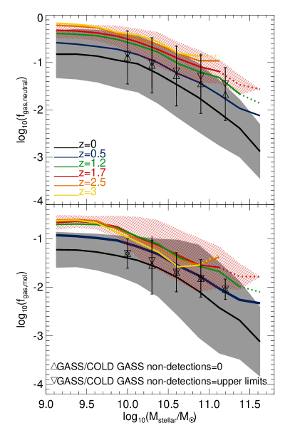
Figure 1: The neutral (Eq. 3; top panel) and molecular (Eq. 4; bottom panel) gas fractions as a function of stellar mass at $z=0$, $z=0.5$, $z=1.2$, $z=1.7$, $z=2.5$, and $z=3$, as labelled, for the eagle simulation. Lines show the median relations, and the hatched regions show the $16^{\rm th}$ to $84^{\rm th}$ percentiles. For clarity, the latter are shown only for $z=0$ and $z=1.7$ galaxies. Solid lines show bins with $>10$ galaxies, while dotted lines show bins where the number of galaxies drops below $10$. Observations at $z=0$ from GASS and COLD GASS are shown using two symbols: upside down triangles show the medians if upper limits are taken for the non detections, and triangles show the median when we set HI and H₂ masses to zero for the non detections. The true median is bracketed by these two values. Errorbars show the $1~{}\sigma$ scatter. eagle and the observations agree within $0.5$ dex.

Fig. 1 shows $f_{\rm gas,neutral}$ and $f_{\rm gas,mol}$ as a function of stellar mass, for all galaxies with $M_{\rm stellar}>10^{9}\,\rm M_{\odot}$ at redshifts $0\leq z\leq 3$ in EAGLE, to match the observed redshift range. Both gas fractions increase with redshift at fixed stellar mass and decrease with stellar mass at a given redshift. The slopes of the relations $f_{\rm gas,neutral}$-stellar mass and $f_{\rm gas,mol}$-stellar mass do not change significantly with redshift, but the normalisations evolve rapidly. The increase of $f_{\rm gas,neutral}$ at fixed stellar mass from $z=0$ to $z\approx 2.5$ is $\approx 0.6$ dex. At $2.5<z<3$, $f_{\rm gas,neutral}$ shows a very weak or no evolution. The molecular gas fraction increases by $\approx 0.6$ dex at fixed stellar mass from $z=0$ to $z\approx 1.2$, which is faster than the evolution of $f_{\rm gas,neutral}$. At $1.7\lesssim z\lesssim 3$, $f_{\rm gas,mol}$ shows little evolution in the stellar mass range $10^{9}\,\rm M_{\odot}\lesssim M_{\rm stellar}\lesssim 5\times 10^{9}\,\rm M_{\odot}$, and a weak decrease with redshift for $M_{\rm stellar}\gtrsim 5\times 10^{9}\,\rm M_{\odot}$. The increase in the neutral and molecular gas fractions from $z=0$ to $z\approx 2$ is due to the increasing accretion rate onto galaxies in the same redshift range. The weak decrease in $f_{\rm gas,mol}$ at $z\gtrsim 2$ is due to galaxies at those redshifts having much higher interstellar radiation fields and lower gas metallicities than galaxies at $z<2$, conditions that hamper the formation of H₂ by dissociating H₂ and reducing the amount of dust available to act as catalyst for H₂, respectively. A significant amount of the gas with densities $>0.1\,\rm cm^{-3}$ remains atomic under these harsh ISM conditions, causing $f_{\rm gas,neutral}$ to continue increase with increasing redshift at fixed stellar mass (at least up to $z\approx 5$), whereas $f_{\rm gas,mol}$ decreases. On average, both $f_{\rm gas,neutral}$ and $f_{\rm gas,mol}$ increase by $\approx 0.6-0.7$ dex from $z=0$ to $z\approx 2$. In the same redshift range, the specific SFR, $\rm sSFR=SFR/M_{\rm stellar}$ increases by a factor of $\approx 15$ (Furlong et al., 2015b) in eagle. This difference between the increase in gas fraction and SFR is a consequence of the super-linear power-law index, $n=1.4$, of the observed star formation law, which is adopted in eagle (Eq. 1; see also discussion in $\S\,5.4$ in Lagos et al. 2015).

In Fig. 1 we also compare the $z=0$ eagle result with the observations of GASS and COLD GASS at $z=0$. The observational strategy in GASS and COLD GASS was to select all galaxies with $M_{\rm stellar}>10^{10}\,\rm M_{\odot}$ at $z<0.05$ from the Sloan Digital Sky Survey Data Release 4 and image a subsample of those in HI and CO(1-0). Catinella et al. (2010) and Saintonge et al. (2011) integrated sufficiently long to enable the detection of HI and H₂ of $>0.015\times M_{\rm stellar}$ at stellar masses $M_{\rm stellar}>10^{10.6}\,\rm M_{\odot}$, or HI and H₂ masses $>10^{8.8}\,\rm M_{\odot}$ in galaxies with $10^{10}\,\rm M_{\odot}<M_{\rm stellar}<10^{10.6}\,\rm M_{\odot}$. In the case of CO observations (for COLD GASS and those discussed below), we adopted a conversion factor $X=2\times 10^{-20}\,\rm cm^{-2}\,(K\,km\,s^{-1})^{-1}$ (Milky-Way like; Bolatto et al. 2013), where X is defined as

$$\frac{N_{\rm H_{2}}}{\rm cm^{-2}}=X\,\left(\frac{I_{\rm CO(1-0)}}{\rm K\,km\,s^{-1}}\right),$$ (5)

where $N_{\rm H_{2}}$ is the H₂ column density and $I_{\rm CO(1-0)}$ is the velocity-integrated $\rm CO(1-0)$ brightness temperature (in traditional radio astronomy observational units). We show the observational results treating non detections in two different ways: by using the upper limits (upside down triangles), and by setting the HI and H₂ masses to zero. eagle results are in qualitative agreement with the observations. The median relations of eagle and GASS plus COLD GASS are at most $0.3$ dex from each other at $M_{\rm stellar}<10^{10}\,\rm M_{\odot}$, while the $1~{}\sigma$ scatter is $\approx 0.5$ dex. There is some tension at $M_{\rm stellar}\gtrsim 10^{11}\,\rm M_{\odot}$, but we show later that this tension is diminished if we study the gas fraction-stellar mass relations in bins of SFR. Lagos et al. (2015) and Bahé et al. (2016) analysed in detail how eagle compares with GASS and COLD GASS, and we point to those papers for more comparisons (e.g. radial profiles, stellar concentrations, SFR efficiencies, etc.).

In Fig. 2 we show the dependence of $f_{\rm gas,neutral}$ and $f_{\rm gas,mol}$ on stellar mass in four bins of SFR. In eagle, both $f_{\rm gas,neutral}$ and $f_{\rm gas,mol}$ show very weak or no evolution at fixed stellar mass and SFR. Thus, the evolution seen in Fig. 1 is related to the increase of the median SFR with redshift at fixed stellar mass. Note that in the top-left panel of Fig. 2 there is a weak evolution of $f_{\rm gas,neutral}$ and $f_{\rm gas,mol}$ with redshift, but this is mostly due to the SFR slightly changing at fixed stellar mass within the allowed range ($0.3\,\rm M_{\odot}\,yr^{-1}<SFR<1\,\rm M_{\odot}\,yr^{-1}$). Galaxies with SFRs closer to $1\,\rm M_{\odot}\,yr^{-1}$ have higher $f_{\rm gas,neutral}$ and $f_{\rm gas,mol}$ than those galaxies having SFRs closer to $0.3\,\rm M_{\odot}\,yr^{-1}$. This means that the weak evolution displayed by eagle in the scaling relations shown in Fig. 2 are simply due to the strong correlation between gas fraction (either neutral or molecular) and SFR. Since the SFR is more strongly correlated with H₂ than with total neutral gas in eagle (Lagos et al., 2015), we see more variations in the $f_{\rm gas,mol}$-stellar mass relation than in the $f_{\rm gas,neutral}$-stellar mass even if we select narrow ranges of SFR (see for example the SFR bin $0.3\rm M_{\odot}\,yr^{-1}<\rm SFR<1\rm M_{\odot}\,yr^{-1}$ in Fig. 2). We come back to this in $\S$ 4.

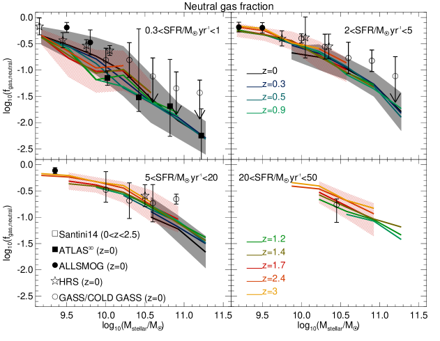
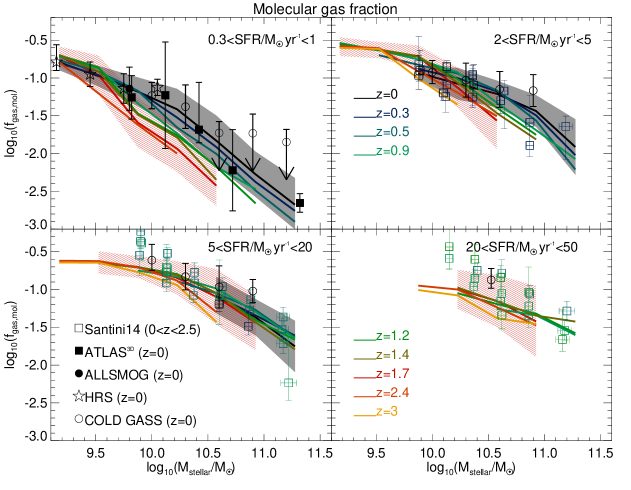
Figure 2: The neutral (Eq. 3; top panels) and molecular (Eq. 4; bottom panels) gas fractions as a function of stellar mass in bins of SFR, as labelled in each panel. For eagle galaxies, lines show the medians, while the $16^{\rm th}$ to $84^{\rm th}$ percentiles are shown as shaded regions (but only for $z=0$ and $z=1.7$ galaxies). We only show bins that have $>10$ galaxies. Symbols show the observational result of GASS and COLD GASS (Catinella et al. 2010 and Saintonge et al. 2011; open circles), HRS (Boselli et al. 2014a; stars), ATLAS^3D (Cappellari et al. 2011; Young et al. 2011; Serra et al. 2012; Davis et al. 2014; filled squares), ALLSMOG (Bothwell et al. 2014; filled circles) and Santini et al. (2014) (open squares). Observations have been coloured according to their redshift following the same colour code we used for eagle galaxies (labelled in the right panels). We see only weak evolution once the gas fraction-stellar mass relation is investigated in bins of SFR, with the remaining evolution being mostly due to evolution of the median SFR within each SFR bin. Overall, eagle agrees well with the observations within $0.3$ dex (with the scatter on the observations being of a similar magnitude).

In Fig. 2 we also show observations from GASS and COLD GASS (Catinella et al. 2010; Saintonge et al. 2011), HRS (Boselli et al. 2014a and Boselli et al. 2014b), the ALLSMOG (Bothwell et al. 2014), ATLAS^3D (Cappellari et al. 2011; Young et al. 2011; Serra et al. 2012; Davis et al. 2014) and from Santini et al. (2014). HRS is a volume-limited survey, containing $323$ galaxies at distances between $15$ and $25$ Mpc, and stellar masses $M_{\rm stellar}\gtrsim 10^{9}\,\rm M_{\odot}$. HRS galaxies were followed-up to image CO(1-0), while HI data was obtained from Giovanelli et al. (2005) and Springob et al. (2005) (see Boselli et al. 2014a for details). ALLSMOG is a survey designed to obtain H₂ masses for galaxies with $3\times 10^{8}\,\rm M_{\odot}\lesssim M_{\rm stellar}\lesssim 10^{10}\,\rm M_{\odot}$, at distances between $40$ and $110$ Mpc. HI data for ALLSMOG was obtained from Meyer et al. (2004), Springob et al. (2005) and Haynes et al. (2011). We use here the first release of Bothwell et al. (2014) of $42$ galaxies. The ATLAS^3D survey is a volume-limited survey of $260$ early-type galaxies with resolved kinematics of the stellar component and ionised gas (Cappellari et al. 2011). Young et al. (2011) and Serra et al. (2012) presented measurements of CO(1-0) and HI masses for ATLAS^3D galaxies, respectively, while stellar masses and SFRs for these galaxies were presented in Cappellari et al. (2013) and Davis et al. (2014), respectively. Santini et al. (2014) presented measurements of $f_{\rm gas,mol}$ as a function of stellar mass in the redshift range $0.1\lesssim z\lesssim 3$. Santini et al. measured dust masses from Herschel photometry, and inferred a gas mass by using measured gas metallicities and a dust-to-gas mass ratio that is metallicity dependent. Since all their sampled galaxies have relatively high SFRs and dust masses, most of the gas mass derived from dust masses is expected to be molecular. We show the observations in bins of SFR, as we did for eagle. Some of the results from GASS and COLD GASS surveys are upper limits due to non-detections of HI and/or CO(1-0). From the observational side, we find broad agreement between the different surveys, even though they cover different stellar mass ranges and redshifts. We emphasise that this is the first demonstration of the stellar mass-SFR-gas fraction connection across redshifts in observational data. This 3-parameter relation is thus a property of real galaxies and hence is a significant observational result.

Fig. 2 shows that EAGLE’s predictions are in good agreement with the observations, within the dispersion of the data and the scatter of the simulation, for all the SFR bins. The median relation of eagle is usually $\lesssim 0.1-0.2$ dex from the median relation in the observations, but this offset of much smaller than the observed scatter ($\approx 0.3-0.5$ dex). For the highest SFR bin ($20\,\rm M_{\odot}\,yr^{-1}<SFR<50\,\rm M_{\odot}\,yr^{-1}$) there is only one observational data point for $f_{\rm gas,neutral}$ due to the lack of HI information. This data point corresponds to the median of $4$ galaxies belonging to GASS and COLD GASS. In the simulation there are no galaxies with those SFRs at $z=0$, which is due to its limited volume. GASS and COLD GASS are based on SDSS, which has a volume at $z<0.1$ that is $\approx 10$ times larger than the volume of the Ref-L100N1504 simulation. Thus, the non existence of such galaxies at $z=0$ in eagle is not unexpected.

From Fig. 2 one concludes that there is a relation between $f_{\rm gas,neutral}$, stellar mass and SFR, and between $f_{\rm gas,mol}$, stellar mass and SFR. These planes exist in both the simulation and the observations, which is a significant result for eagle and observations. This motivates us to analyse more in detail how fundamental these correlations are compared to the more widely-known scaling relations introduced in $\S$ $1$. With this in mind we perform a principal component analysis in the next section.

4 The fundamental plane of star formation

4.1 A principal component analysis

With the aim of exploring which galaxy correlations are most fundamental and how the gas fraction-SFR-stellar mass relations fit into that picture, we perform a principal component analysis (PCA) over $7$ properties of galaxies in the Ref-L100N1504 simulation. We do not include redshift in the list of properties because we decide to only include properties of galaxies to make the interpretation of PCA more straightforward. However, we do analyse possible redshift trends in $\S$ 4.2. We include all galaxies in eagle with $M_{\rm stellar}>10^{9}\rm M_{\odot}$, SFR$>0.01\,\rm M_{\odot}\,yr^{-1}$, $M_{\rm neutral}>10^{7}\rm\,M_{\odot}$ and at $0\leq z\leq 4.5$ in the PCA. Here $M_{\rm neutral}$ is the HI plus H₂ mass. The PCA uses orthogonal transformations to find linear combinations of variables.

PCA is designed to return as the first principal component the combination of variables that contains the largest possible variance of the sample, with each subsequent component having the largest possible variance under the constraint that it is orthogonal to the previous components. In order to perform the PCA, we renormalise galaxy properties in logarithmic space by subtracting the mean and dividing by the standard deviation of each galaxy property. Table 2 shows the variables that were included in the PCA and shows the first three principal components. We apply equal weights to the galaxies in the PCA, which is justified by the fact that the redshift distribution of galaxies with $M_{\rm stellar}>10^{9}\,\rm M_{\odot}$ is close to flat (see bottom panel of Fig. 5).

Table 2: Principal component analysis (PCA) of galaxies in the Ref-L100N1504 simulation. Galaxies with $M_{\rm stellar}>10^{9}\,\rm M_{\odot}$, $\rm SFR>0.01\,M_{\odot}\,yr^{-1}$, $M_{\rm H_{2}}/(M_{\rm H_{2}}+M_{\rm stellar})>0.01$ and $0\leq z\leq 4.5$ were included in the analysis. The PCA was conducted with the variables: stellar mass, star formation rate, metallicity of the star-forming gas ($Z_{\rm SF,gas}$), molecular, atomic and neutral gas masses and the half-mass stellar radius $r_{\rm 50,st}$. We adopt $Z_{\odot}=0.0127$. Before performing the PCA, we renormalise all the components by subtracting the mean and dividing by the standard deviation (all in logarithm). In the table we show the property each component relates to, but we remind the reader that we renormalise them before performing the PCA. The three first principal components account for $55$% $24$% and $14$%, respectively, of the total variance, and therefore account together for $93$% of the total variance. The first three PCA vectors are shown here.

	(1)	(2)	(3)	(4)	(5)	(6)	(7)
comp.	$\hat{\rm x}_{1}$	$\hat{\rm x}_{2}$	$\hat{\rm x}_{3}$	$\hat{\rm x}_{4}$	$\hat{\rm x}_{5}$	$\hat{\rm x}_{6}$	$\hat{\rm x}_{7}$
Prop.	$\rm log_{10}\left(\frac{M_{\rm stellar}}{\rm M_{\odot}}\right)$	$\rm log_{10}\left(\frac{SFR}{M_{\odot}\,yr^{-1}}\right)$	$\rm log_{10}\left(\frac{Z_{\rm SF,gas}}{Z_{\odot}}\right)$	$\rm log_{10}\left(\frac{M_{\rm H_{2}}}{\rm M_{\odot}}\right)$	$\rm log_{10}\left(\frac{M_{\rm HI}}{\rm M_{\odot}}\right)$	$\rm log_{10}\left(\frac{M_{\rm neutral}}{\rm M_{\odot}}\right)$	$\rm log_{10}\left(\frac{\rm r_{\rm 50,\star}}{\rm kpc}\right)$
PC1	$0.31$	$-0.57$	$-0.19$	$-0.15$	$0.4$	$0.6$	$0.06$
PC2	$0.46$	$0.04$	$-0.31$	$-0.51$	$0.22$	$-0.61$	$0.09$
PC3	$-0.19$	$-0.68$	$-0.14$	$0.33$	$-0.33$	$-0.51$	$0.002$

We find that the first principal component is dominated by the stellar mass, SFR and the neutral gas mass (and secondarily by the atomic gas mass), with weaker dependencies on the molecular gas mass and the gas metallicity. This component accounts for 55% of the variance of the galaxy population. The relation between the neutral gas fraction, SFR and stellar mass of galaxies define a plane in the 3-dimensional space, which we refer to as “the fundamental plane of star formation”, that we explore in detail in $\S$ 4.2. Since this plane accounts for most of the variance, it is one of the most fundamental relations of galaxies. This is an important prediction of eagle.

The second principal component is dominated by the stellar mass, metallicity of the star-forming gas, and molecular and neutral gas masses. This component is responsible for $24$% of the variance of the galaxy population in eagle, and can be connected with the mass-metallicity relation and how its scatter is correlated with the molecular and neutral gas content. Note that molecular gas plays a secondary role compared to the neutral gas fraction. This will be discussed in $\S$ 4.3.

The third principal component shows a correlation between all the gas components (molecular, atomic and neutral), SFR and secondarily on stellar mass and gas metallicity. This principal component shows that galaxies tend to be simultaneously rich (or poor) in atomic and neutral (molecular plus atomic) hydrogen. Note that the half-mass radius does not strongly appear in the first three principal components. We find that $r_{\rm 50,\star}$ appears in the fourth and fifth principal components, with dependencies on the stellar mass and molecular gas mass (no dependence of $r_{\rm 50,\star}$ on gas metallicity is seen in our analysis).

We test how the PCA is affected by selecting subsamples of galaxies. Selecting galaxies with $M_{\rm stellar}>10^{10}\,\rm M_{\odot}$ has the effect of increasing the importance of the H₂ mass and metallicity on the first principal component, while in the second principal component we see very little difference. However, we still see that the main properties defining the first principal component are the stellar mass, SFR and neutral gas mass. If instead, we select galaxies with $M_{\rm stellar}>10^{9}\,\rm M_{\odot}$ that are mostly passive (those with $\rm 0.001\,M_{\odot}\,yr^{-1}\leq SFR\leq 0.1\,M_{\odot}\,yr^{-1}$), we find that the first principal component changes very little, while in the second principal component $M_{\rm H_{2}}$ becomes as important as $M_{\rm neutral}$. A selection of galaxies with $M_{\rm stellar}>10^{10}\,\rm M_{\odot}$ and $\rm 0.001\,M_{\odot}\,yr^{-1}\leq SFR\leq 0.1\,M_{\odot}\,yr^{-1}$ (which again correspond to mostly passive galaxies), produces the PCA to give more weight to the gas metallicity and the H₂ mass in the first principal component, becoming more dominated by the stellar mass, SFR, $Z_{\rm SF,gas}$ and H₂ and HI masses. These tests show that the first principal component is always related to the fundamental plane of star formation that we introduce in $\S$ 4.2 regardless of whether we select massive galaxies only, passive galaxies or the entire galaxy population. For galaxies with SFRs$\lesssim 0.1\,\rm M_{\odot}\,yr^{-1}$, we see that the metallicity becomes more prominent in the first principal component. The second principal component in all the tests we did has the gas metallicity playing an important role and therefore is always related to the MZ relation.

As an additional test to determine which gas phase is more important (neutral, atomic or molecular), we present in Appendix B three principal component analyses, in which we include stellar mass, SFR, gas metallicity and HI, H₂ or neutral gas mass. We find that the highest variance is obtained in the first principal component of the PCA that includes the neutral gas mass. If instead we include the HI or H₂ masses, we obtain a smaller variance on the first principal component. In addition, we find that the contribution of the metallicity of the star-forming gas in the first principal components of the PCA performed using the neutral or HI gas masses is negligible, while it only appears to be important if we use the H₂ mass instead. This supports our interpretation that most of the variance in the galaxy population is enclosed in the “the fundamental plane of star formation” of galaxies, and that the neutral gas mass is more important than the HI or H₂ masses alone. In the rest of this section we analyse in detail the physical implications of the first two principal components presented in Table 2, which together account for $79$% of the variance seen in the EAGLE galaxy population.

4.2 The fundamental plane of star formation

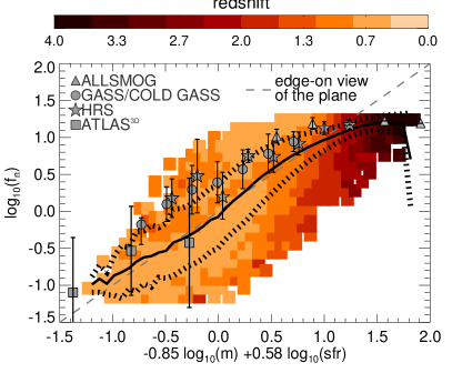
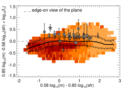
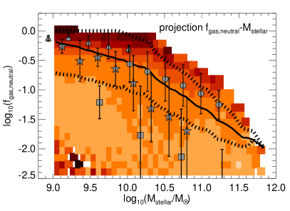
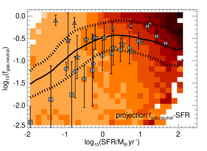
Figure 3: Four views of the distribution of galaxies in the 3-dimensional space of neutral fraction, stellar mass and SFR. We include all eagle galaxies with $M_{\rm stellar}>10^{9}\,\rm M_{\odot}$, in the redshift range $0\leq z\leq 4.5$. The median and $16^{\rm th}$ and $84^{\rm th}$ percentiles are shown as solid and dotted lines, respectively, and are shown in all the panels. Filled squares are coloured according to the median redshift of galaxies in bins of the horizontal and vertical axis, as indicated in the colour bar. The top panels show edge-on views of the fitted plane of Eq. 6, with the top-left panel showing normalised gas fraction as a function of the combination of SFR and stellar mass of Eq. 6 (see also Eq. 8 for the definitions of m, sfr and f_n), while the top-right panel shows the vector perpendicular to the plane, $\rm\vec{v}_{\perp}=(a,b,c)$, as a function of a vector parallel to the plane, $\rm\vec{v}_{\parallel}=(-b,-a,0)$, where the plane is defined as $\rm ax+by+cz=0$ (see Eq. 6). The bottom panels show two projections along the axes of the 3-dimensional space that are nearly face-on views of the plane: $f_{\rm gas,neutral}$ vs. stellar mass (left panel) and $f_{\rm gas,neutral}$ vs. SFR (right panel). The dashed line in the top panels show edge-on views of the plane. Symbols show observations: squares correspond to GASS and COLD GASS, circles to HRS, squares to ATLAS^3D, and triangles to the ALLSMOG survey, as labelled in the top-left panel. Observations follow a plane in the 3-dimensional space of $f_{\rm gas,neutral}$, stellar mass and SFR that is very similar to the one predicted by eagle. For a movie rotating over the 3-dimensional space please see www.clagos.com/movies.php.

Here we investigate the dependence of the neutral and molecular gas fraction on stellar mass and SFR. We change from using gas masses in $\S$ 4.1 to gas fractions. The reason for this is that the scatter in the 3-dimensional space of stellar mass, SFR and neutral gas fraction or molecular gas fraction is the least compared to what it is obtained if we instead use gas masses or simply neutral or molecular gass mass to stellar mass ratios. We come back to this when discussing Eqs. 6 and 7.

In order to visualise a flat plane in a three-dimensional space, it helps to define vectors that are perpendicular and parallel to the plane, and plot them against each other in order to reveal edge-on and face-on orientations of the plane. This is what we do in this section. If we define a plane as $\rm ax+by+cz=0$, vector perpendiculars and parallel to the plane would be $\rm\vec{v}_{\perp}=(a,b,c)$ and $\rm\vec{v}_{\parallel}=(-b,-a,0)$, respectively. We use these vectors later to show edge-on orientations of the fundamental plane of star formation, which we introduce in Eqs. 6 and 7.

Fig. 3 shows four views of the 3-dimensional space of neutral gas fraction, stellar mass and SFR. In this figure we include all galaxies in eagle with $M_{\rm stellar}>10^{9}\,\rm M_{\odot}$, SFR$\geq 0.01\rm\,M_{\odot}\,yr^{-1}$, and that are in the redshift range $0\leq z\leq 4.5$. We show the underlying redshift distribution of the galaxies by binning each plane and colouring bins according to the median redshift of the galaxies. Two of the views show edge-on orientations of the plane (i.e. with respect to the best-fit plane of Eq. 6 below), and the other two are projections along the axes of the 3-dimensional space. One edge on view (top-left panel) shows the neutral gas fraction as a function of the combination of SFR and stellar mass of Eq. 6. For the second edge-on view (top-right panel), we use the perpendicular and parallel vectors defined above, with the plane being defined in Eq. 6.

Galaxies populate a well-defined plane, which shows little evolution. Galaxies evolve along this plane with redshift, in such a way that they are on average more gas rich and more highly star-forming at higher redshift. When we consider the molecular gas fraction instead of the neutral gas fraction, the situation is the same: galaxies populate a well-defined plane in the 3-dimensional space of $f_{\rm gas,mol}$, stellar mass and SFR (shown in Fig. 4). This means that at fixed SFR and stellar mass, there is very little evolution in $f_{\rm gas,neutral}$ and $f_{\rm gas,mol}$. Hence, most of the observed trend of an increasing molecular fraction with redshift (e.g. Geach et al. 2011; Saintonge et al. 2013) is related to the median SFR at fixed stellar mass increasing with redshift (e.g. Noeske et al. 2007; Sobral et al. 2014). We argue later that both the SFR and gas fraction are a consequence of the self-regulation of star formation in galaxies.

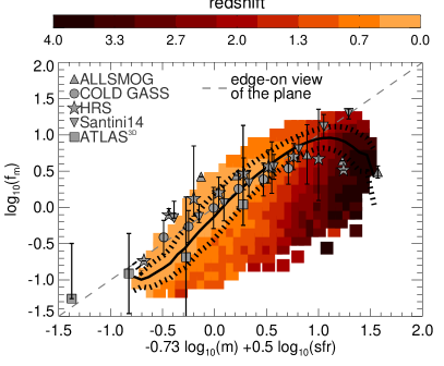
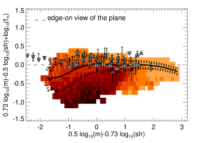
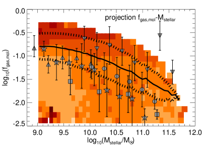
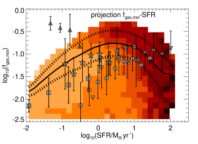
Figure 4: As in Fig. 3 but for the molecular gas fraction. For the two edge-on views of the top panels we use the plane definition of Eq. 7 (see also Eq. 8 for the definitions of m, sfr and f_m). Here we also show the observational results from Santini et al. (2014), which correspond to star-forming galaxies at $z\lesssim 3$. For a movie rotating over the 3-dimensional space please see www.clagos.com/movies.php.

For both $f_{\rm gas,neutral}$ and $f_{\rm gas,mol}$ the relation is best described by a curved surface in 3-dimensional space. Here we provide fits of the flat plane tangential to this 2-dimensional surface at $M_{\rm stellar}=5\times 10^{10}\,\rm M_{\odot}$ and $\rm SFR=2\,M_{\odot}\,yr^{-1}$, which we compute using the HYPER-FIT R package of Robotham & Obreschkow (2015). We refer to the tangential plane fitted to the $\rm f_{\rm gas,neutral}-SFR-M_{\rm stellar}$ relation as “the fundamental plane of star formation”. For the fitting, we weigh each galaxy by the inverse of the number density in logarithmic mass interval in order to prevent the fit from being biased towards the more numerous small galaxies. The best fit planes are:

$$0.85\,{\rm log_{10}(m)}-0.58\,{\rm log_{10}(sfr)}+{\rm log_{\rm 10}(f_{\rm n})} = 0,$$ (6)

$$0.73\,{\rm log_{10}(m)}-0.50\,{\rm log_{10}(sfr)}+{\rm log_{\rm 10}(f_{\rm m})} = 0,$$ (7)

where,

$${\rm m} = \frac{M_{\rm stellar}}{5\times 10^{10}\,\rm M_{\odot}},\,\,{\rm sfr}=\frac{{\rm SFR}}{\rm 2\,M_{\odot}\,yr^{-1}},\,$$

$$f_{\rm n} = \frac{f_{\rm gas,neutral}}{0.046},\,\,\,\,\,\,\,f_{\rm m}=\frac{f_{\rm gas,mol}}{0.026}.$$ (8)

The fits above are designed to minimise the scatter. The best fits of Eqs. 6 and 7 are shown as dashed lines in the top-left panels of Fig. 3 and Fig. 4, respectively. The standard deviations perpendicular to the planes calculated by HYPER-FIT are $0.17$ dex for Eq. 6 and $0.15$ dex for Eq. 7, while the standard deviations parallel to the gas fraction axis are $0.24$ dex for Eq. 6 and $0.2$ dex for Eq. 7. Although the scatter seen for the molecular gas fraction is slightly smaller than for the neutral gas fraction, the PCA points to the latter as capturing most of the variance of the galaxy population. This is because the neutral gas fraction is more directly connected to the process of gas accretion than the molecular gas fraction, and we discuss later that accretion is one of the key processes determining the existence of the fundamental planes. In addition, because SFR and the molecular gas mass are strongly correlated, only one of these properties is needed to describe most of the variance among galaxy properties. We also analysed the correlation between $f_{\rm gas,neutral}$ ($f_{\rm gas,mol}$) and specific SFR, and found that the scatter increases by $\approx 20$% ($\approx 25$%) relative to the scatter characterising Eq. 6. We find that fitting planes to the three-dimensional dependency of gas mass-SFR-stellar mass or gas-to-stellar mass ratio-SFR-stellar mass (instead of gas fraction-SFR-stellar mass, as presented in Eqs. 6 and 7) lead to an increase in the scatter relative to was it is obtained around Eqs. 6 and 7 of $\approx 20-30$%. We therefore conclude that the tightest correlations (i.e. least scatter) in eagle are those between gas fraction, stellar mass and SFR.

Note that there is a clear turnover at $f_{\rm gas,mol}\approx 0.3$ (very clear at a y-axis value $\approx 0.7$ in the top-left of Fig. 4), which is produced by galaxies with $\rm SFR\gtrsim 15\,\rm M_{\odot}\,yr^{-1}$. Most of the galaxies that produce this turnover are forming stars in an ISM with a very high median pressure (SFR-weighted pressures of $\rm log_{10}(\langle P\rangle\,k^{-1}_{B}/\,\rm cm^{-3}\,K)\approx 6-7$). The turnover is less pronounced in the neutral gas fraction relation (top left panel in Fig. 3). Most galaxies that lie around the turn-over are at $z\gtrsim 2$. The fact that we do not see such strong turn-over in the neutral gas fraction is because galaxies with high SFRs have an intense radiation field that destroys H₂ more effectively, moving the HI to H₂ transition towards higher gas pressures. Thus, a significant fraction of the gas with densities $n_{\rm H}\gtrsim 1\,\rm cm^{-3}$ remains atomic at high-redshift. The effect of this on the H₂ fraction is important, introducing the turn-over at high H₂ fractions seen in Fig. 4.

For the neutral gas fraction we find that the fitted plane of Eq. 6 is a good description of the neutral gas fractions of galaxies in eagle (note that this is also true for the higher resolution simulations shown in Appendix A) at $f_{\rm gas,neutral}\lesssim 0.5$ (y-axis value $\approx 1$ in the top-left of Fig. 3). However, at higher neutral gas fractions, the fit tends to overshoot the gas fraction by $\approx 0.1-0.2$ dex. The latter is not because the gas fraction saturates at $\approx 1$, but because there is a physical change in the ratio of SFR to neutral gas mass from $z=0$ towards high redshift, due to the super-linear star formation law adopted in eagle and the ISM gas density evolution. We come back to this point in $\S$ 4.2.1. For the molecular gas fraction we find that the fit of Eq. 7 describes the molecular gas fractions of eagle galaxies well in the regime $0.02\lesssim\rm f_{\rm gas,mol}\lesssim 0.3$ ($-0.2\lesssim\rm log_{10}(f_{m})\lesssim 1$), while at lower and at higher $f_{\rm gas,mol}$ the fit overshoots the true values of the gas fraction. At the high molecular gas fractions this is due to galaxies populating the turnover discussed above, that deviates from the main plane (which corresponds to galaxies with SFR$\gtrsim\rm 15\,M_{\odot}\,yr^{-1}$ and $f_{\rm gas,mol}\lesssim 0.3$).

We also investigated the distribution of eagle galaxies in the 3-dimensional space of star-forming gas mass, $M_{\rm stellar}$ and SFR at higher redshifts, $5\leq z\leq 7$. We used star-forming gas mass rather than neutral or molecular gas mass, because our approximations for calculating the latter two may not be accurate at these higher redshifts (see e.g. the discussion in Rahmati et al. 2013b). We find that $5\leq z\leq 7$ eagle galaxies trace a 2-dimensional curved surface in this 3-dimensional space with little scatter. This leads us to suggest that the process that induces the strong correlation that gives rise to the fundamental plane of star formation at $z\leq 4.5$, is already operating at $5\leq z\leq 7$.

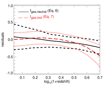
Figure 5: Top panel: Residuals of simulated galaxies from Eqs. 6 and 7 as a function of $\rm log_{\rm 10}(1+redshift)$. Here residuals are defined as $\rm ax+by+cz$, where $a$, $b$ and $c$ are defined in Eqs. 6 and 7. The solid black line is the mean residual of galaxies with $M_{\rm stellar}>10^{9}\,\rm M_{\odot}$ from the fit of Eq. 6 to the fundamental plane, with the dashed lines indicating the $16^{\rm th}$ and $84^{\rm th}$ percentiles. The red long dashed line and red dotted lines, are the corresponding median and percentiles residuals from the fit of Eq. 7. Note that the redshift at which the medians cross zero is set by the choice of normalisation, and thus it has no physical meaning. Bottom panel: Redshift distribution of the galaxies with $M_{\rm stellar}>10^{9}\,\rm M_{\odot}$i, shown at the top panel.

We show in Fig. 5 the residuals of the galaxies from the fits of Eqs. 6 and 7 as a function of redshift. In the case of Eq. 6, we see that residuals depend very weakly on redshift, with the median slightly decreasing with increasing redshift. Including redshift in HYPER-FIT leads to an increase in the scatter of $\approx 50$%, indicating that including redshift does not improve the fit provided in Eq. 6. For the molecular gas fraction fit of Eq. 7, we find the residuals show no dependence with redshift at $z<2$ ($\rm log_{\rm 10}(1+redshift)\approx 0.5$), and the trend seen at higher redshifts is due to the turnover discussed above. Again, we observe an increase in the scatter of the fit if we include redshift, showing that there is no improvement by adding redshift (unless we ignore galaxies at $z<2$).

In Figs. 3 and 4 we also investigate whether observed galaxies populate a similar plane in the gas fraction, stellar mass and SFR space, as the one eagle predicts. The observational datasets, which were introduced in $\S$ 3, correspond to GASS, COLD GASS, HRS, ALLSMOG, ATLAS^3D and Santini et al. (2014).

We show the observations in Figs. 3 and 4 in the same way as we show eagle results: we calculate the median neutral and molecular gas fraction and the 1$\sigma$ scatter around those values in the two edge-on views with respect to the best fits of Eqs. 6 and 7, and the two projections over the axis of the 3-dimensional space. We find that observed galaxies follow a similar plane as galaxies in eagle, albeit with some surveys having neutral gas fractions $\approx 0.1-0.2$ dex higher than those found for eagle galaxies at fixed stellar mass and SFR. For example if we compare eagle with GASS plus COLD GASS, we find such an offset in the neutral gas fractions, but compared to HRS and ATLAS^3D we find very good agreement. Regarding molecular fractions, we find that the observations follow a plane that is very similar to the one described by the eagle galaxies, as shown in Fig. 4. Interestingly, the observations suggest a turn-over at high $f_{\rm gas,mol}$ similar to the one displayed by eagle (see top-left panel of Fig. 4). This could point to real galaxies forming stars in intense UV radiation fields, as we find for eagle galaxies.

Overall, we find that the agreement with the observations is well within the scatter of both the simulation and observations. Note that galaxies in the observational sets used here were selected very differently and in some cases using complex criteria, which is easy to see in the nearly face-on views of the bottom panels of Fig. 3 and Fig. 4. For example, ATLAS^3D and ALLSMOG differ by $\gtrsim 1.5$ dex in the nearly face-on views. However, when the plane is seen edge-on, both observational datasets follow the same relations. This means that even though some samples are clearly very biased, like Santini et al. (2014) towards gas-rich galaxies, when we place them in the 3-dimensional space of gas fraction, SFR and stellar mass, they lie on the same plane. The fact that observations follow a very similar plane in the 3-dimensional space of gas fraction, SFR and stellar mass as eagle is remarkable.

4.2.1 Physical interpretation of the fundamental plane of star formation

We argue that the existence of the 2-dimensional surfaces in the 3-dimensional space of stellar mass, SFR and neutral or molecular gas fractions in eagle is due to the self-regulation of star formation in galaxies. The rate of star formation is controlled by the balance between gas cooling and accretion, which increase the gas content of galaxies, and stellar and BH-driven outflows, that remove gas out of galaxies (see Schaye et al. 2010, Lagos et al. 2011, Booth & Schaye 2010, Haas et al. 2013a for numerical experiments supporting this views). In this picture, both the gas content and the SFR of galaxies change to reflect the balance between accretion and outflows, and the ratio is determined by the assumed star formation law.

This interpretation is supported by the comparison of the reference model we use here with model variations in eagle presented in Appendix C. We show $4$ models in which the efficiency of AGN and stellar feedback is changed. We find that weakening the stellar feedback has the effect of changing the normalisation of the plane, but most importantly, increasing the scatter around it, while making feedback stronger tends to tighten the plane. The effect of AGN feedback is very mild due to most of the galaxies shown being on the main sequence of galaxies in the SFR-$M_{\rm stellar}$ plane, and therefore not affected by AGN feedback. A similar change in scatter is seen if we now look at models where the stellar feedback strength has a different scaling (i.e. depending on metallicity alone or on the velocity dispersion of the dark matter). Both model variations produce less feedback at higher redshift ($z>1$; see Fig. $5$ in C15) compared to the reference model, which leads to both models producing a more scattered ‘fundamental plane of star formation’ at high redshift. If feedback was not sufficient to balance the gas inflows, the scatter would increase even further, erasing the existence of the fundamental plane of star formation discussed here.

We find that the curvature of the 2-dimensional surface is mainly driven by how the gas populates the probability distribution function (PDF) of densities in galaxies at different redshifts and how star formation depends on the density in eagle (see $\S$ 2.1). Galaxies at high redshift tend to form stars at higher ISM pressures than galaxies at $z=0$, on average (see Fig. $12$ in Lagos et al. 2015), which together with the super-linear star formation law, lead to higher-redshift galaxies having higher star formation efficiencies (i.e. the ratio between the SFR and the gas content above the density threshold for star formation). In Appendix C we show that changing the dependency of the SFR density on the gas density changes the slope of the plane significantly, supporting our interpretation.

4.2.2 Example galaxies residing in the fundamental plane of star formation

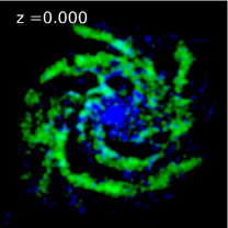
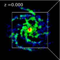
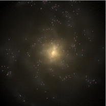
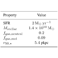
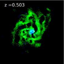
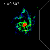
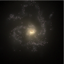
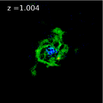
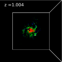
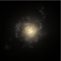
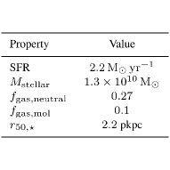
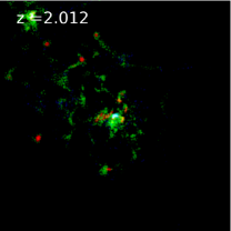
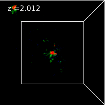
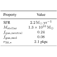
Figure 6: Visualisation of $4$ galaxies in eagle (at redshifts $z=0$, $z=0.5$, $z=1$ and $z=2$) which were chosen to have $M_{\rm stellar}\approx 10^{10}\rm M_{\odot}$, $\rm SFR\approx 2\rm\,M_{\odot}\,yr^{-1}$ and $f_{\rm gas,neutral}\approx 0.25$. The redshift of each galaxy is shown in the HI and H₂ maps. The HI and H₂ maps are coloured by column density, according to the colour bars at the top, with column densities in units of $\rm cm^{-2}$. The right panels show SDSS gri images, which were constructed using the radiative transfer code SKIRT (Baes et al., 2011) (see Trayford et al. in prep. for details). Particles are smoothed by $1$ ckpc in the $N_{\rm H_{2}}$ and $N_{\rm HI}$ maps. HI and H₂ maps have a size of $100\times 100$ pkpc², while the gri images are of $60\times 60$ pkpc² (scale that is shown in the middle panels as a white square frame). At the right of every row we show the integrated values for the stellar mass, SFR, neutral gas fraction, molecular gas fraction and the projected half-stellar mass radius. Masses and SFR were calculated in spherical apertures of $30$ pkpc, while the radius is calculated using a 2D circular aperture of $30$ pkpc (averaged over three orthogonal projections).

We select examples of galaxies of a similar stellar mass, SFR and neutral gas fraction at different redshifts to examine their similarities and differences. Fig. 6 shows the atomic and molecular column density maps and the optical gri images of $4$ galaxies at $z=0$, $0.5$, $1.0$ and $2$ with $M_{\rm stellar}\approx 1.1\times 10^{10}\,\rm M_{\odot}$, $\rm SFR\approx 2\,\rm M_{\odot}\,yr^{-1}$ and $f_{\rm gas,neutral}\approx 0.2$. The optical images were created using radiative transfer simulations performed with the code SKIRT (Baes et al., 2011) in the SDSS g, r and i filters (Doi et al., 2010). Dust extinction was implemented using the metal distribution of galaxies in the simulation, and assuming $40$% of the metal mass is locked up is dust grains (Dwek, 1998). The images were produced using particles in spherical apertures of $30$ pkpc around the centres of sub-halos (see Trayford et al. 2015, and in prep. for more details).

At $z=0$, $\rm SFR\approx 2\,\rm M_{\odot}\,yr^{-1}$ and $f_{\rm gas,neutral}\approx 0.2$ are typical values of galaxies with $M_{\rm stellar}\approx 10^{10}\,\rm M_{\odot}$ in the main sequence of star formation. However, at higher redshifts, the normalisation of the sequence increases, and therefore a galaxy with the stellar mass, SFR and neutral gas fraction above lies below the main sequence of star formation and is thus considered an unusually passive galaxy. Nonetheless, it is illuminating to visually inspect galaxies of the same properties at different redshifts.

We find that the $z=0$ galaxy in Fig. 6 is an ordered disk (which is a common feature of galaxies with these properties at $z=0$), with most of the star formation proceeding in the inner parts of the galaxy and in the disk (compare H₂ mass with stellar density maps). However, in the $z=0.5$ and $z=1$ galaxies we see striking differences: the higher-redshift galaxies are smaller (see the values of their half-mass radius listed in Fig. 6), have more disturbed disks, have steeper H₂ density profiles, and are more clumpy. This is particularly evident when we compare the $z=0$ galaxy with its $z=1$ counterpart with the same integrated properties. The picture at $z=2$ again changes completely: the neutral gas of the $z=2$ galaxy displays a very irregular morphology with filaments at $\approx 50-100$ pkpc from the galaxy centre, which is much more evident in HI than in H₂, but still present in the latter. In the $z=2$ galaxy, a significant fraction of the H₂ is locked up in big clumps, which is in contrast with the smooth distribution of H₂ in the $z=0$ galaxy.

Although galaxies follow a tight plane relating $f_{\rm gas,neutral}$, stellar mass and SFR with little redshift evolution, they can have strikingly different morphologies even at fixed $f_{\rm gas,neutral}$, stellar mass and SFR. We analyse this in detail in an upcoming paper (Lagos et la. in prep.).

4.3 The Mass-Metallicity relation

The PCA performed with eagle galaxies shows that the mass-metallicity relation emerges mostly in the second principal component (that accounts for $24$% of all the variance seen in the galaxy population of the simulation). However, the relation between stellar mass and gas metallicity is not so strong, and other variables are also relevant in the principal component, such as SFR and gas mass. We find that the neutral gas fraction again plays a more important role than the molecular gas fraction. Here we analyse in detail this multi-dimensional scaling.

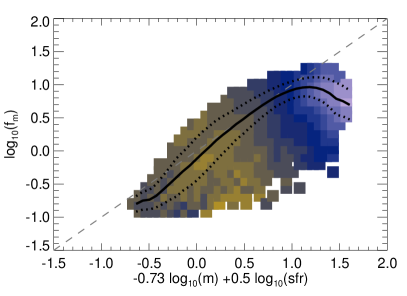
Figure 7: Top panel: As in the top-left panel of Fig. 3, but here we colour pixels by the metallicity of the star-forming gas, as the colour bar at the top of the panel shows. Bottom panel: As in the top-left panel of Fig. 4, but here we colour pixels by the metallicity of the star-forming gas. For movies rotating over the 3-dimensional spaces see www.clagos.com/movies.php. The dashed lines in both panels show the one-to-one relationship (i.e. best fits of Eqs. 6 and 7).

Fig. 7 shows edge-on views of the planes in the space comprising $f_{\rm gas,neutral}$ or $f_{\rm gas,mol}$ and stellar mass and SFR (defined as in Eqs. 6 and 7, respectively). All galaxies in the redshift range $0\leq z\leq 4.5$ and with $M_{\rm stellar}>10^{9}\rm\,M_{\odot}$ were included in the figure. Pixels are coloured according to the median star-forming gas (i.e. ISM) metallicity, as indicated by the colour bar. Gas metallicity decreases as the neutral gas fraction increases at fixed x-axis value. Galaxies with high neutral gas fractions and high SFRs are almost exclusively metal poor. For example, galaxies with $\rm SFR>15\rm\,M_{\odot}\,yr^{-1}$ and $f_{\rm gas,neutral}>0.7$ have a median metallicity of the star-forming gas of $Z_{\rm SF,gas}\approx 0.3\,\rm Z_{\odot}$. For galaxies with slightly lower SFRs, $\rm 10\rm\,M_{\odot}\,yr^{-1}<SFR<15\rm\,M_{\odot}\,yr^{-1}$ and $0.4<f_{\rm gas,neutral}<0.6$, the median metallicity of the star-forming gas is $Z_{\rm SF,gas}\approx 0.8\,\rm Z_{\odot}$. The trend of decreasing metallicity with increasing gas fraction is not driven by how galaxies at different redshift populate the plane, given that the metallicity trend of Fig. 7 is still seen at fixed redshift (this is not shown in Fig. 7). Note that the direction in which the metallicity of the star-forming gas changes is orthogonal to the plane defined by Eq. 6. Galaxies with $\rm log_{10}(f_{n})\gtrsim 1$, that are among the most metal-poor galaxies in EAGLE, lie in the region where the relation in the top panel of Fig. 7 flattens. These galaxies correspond to star-forming dwarf galaxies in EAGLE (which have SFR$\approx 2-3\,\rm M_{\odot}\,yr^{-1}$, $M_{\rm stellar}\approx 2\times 10^{9}\rm M_{\odot}$ and $f_{\rm gas,neutral}\gtrsim 0.5$).

Galaxies with high molecular gas fractions also tend to be more metal poor than galaxies with lower $f_{\rm gas,mol}$. For example, galaxies with $\rm SFR>15\rm\,M_{\odot}\,yr^{-1}$ and $f_{\rm gas,mol}>0.3$ have a median metallicity of the star-forming gas of $Z_{\rm SF,gas}\approx 0.6\,\rm Z_{\odot}$. For galaxies with slightly lower SFRs, with $\rm 10\rm\,M_{\odot}\,yr^{-1}<SFR<15\rm\,M_{\odot}\,yr^{-1}$ and $0.1<f_{\rm gas,mol}<0.2$, the median metallicity of the star-forming gas is $Z_{\rm SF,gas}\approx 1.2\,\rm Z_{\odot}$. However, the direction of the correlation here is different to the one found for $f_{\rm gas,neutral}$. The metallicity of the star-forming gas decreases parallel to the plane of Eq. 7, which means that little extra information is gained through adding gas metallicity as an extra dimension in the dependence $f_{\rm gas,mol}$-stellar mass-SFR.

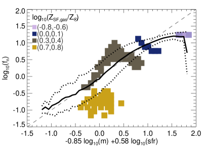
Figure 8: As in the top panel of Fig. 7 but here we show 4 discrete bins in metallicity, as labelled. Galaxies in a narrow range of metallicity occupy well defined regions of the fundamental plane of star formation.

In order to help visualise this more clearly, we show in Fig. 8 the same edge-on view of the top panel of Fig. 7 but for four narrow bins of star-forming gas metallicity. We see that narrow ranges in metallicity result in a very small portion of the plane being sampled. This implies that the position of the galaxy on the plane comprised of $f_{\rm gas,neutral}$, stellar mass and SFR is a good proxy for the star-forming gas metallicity. A consequence of this is that the scatter in the SFR or neutral gas fraction largely determines the scatter in the stellar mass-gas metallicity relation. This agrees with recent claims by Zahid et al. (2014), which based on observations and a simple model of chemical enrichment, claim that gas metallicity is strongly correlated with the gas fraction, with the latter relation not evolving in time.

We find that the gas metallicity in eagle is more strongly correlated with the neutral gas fraction than with the molecular gas fraction. Recently, Bothwell et al. (2015), using a sample comprising $221$ galaxies in the redshift range $0\leq z\leq 2$, claimed that the residuals of the MZ relation are more strongly correlated with H₂ than SFR. However, due to the lack of data, Bothwell et al. were not able to test whether atomic hydrogen or neutral hydrogen masses are better predictions of the scatter than the H₂ mass.

We use the HYPER-FIT R package of Robotham & Obreschkow (2015) to fit the dependence of $Z_{\rm SF,gas}$ on stellar mass, SFR and $f_{\rm gas,neutral}$ and find that the least scatter $3$-dimensional surface has a very weak dependence on stellar mass and SFR, and a strong dependence on $f_{\rm gas,neutral}$. This means that the metallicity of the star-forming gas in galaxies can be predicted from the neutral gas fraction alone to within $40$%. We perform these fits independently of Eqs. 6 and 7. The best fit between $Z_{\rm SF,gas}$ and $f_{\rm gas,neutral}$ is:

$${\rm log_{\rm 10}}\left(\frac{Z_{\rm SF,gas}}{Z_{\odot}}\right) = -0.57\,{\rm log_{\rm 10}}\left(\frac{f_{\rm gas,neutral}}{0.09}\right).$$ (9)

The standard deviation perpendicular to the fitted relation of Eq. 9 is $0.17$ dex, while the standard deviation parallel to the metallicity axis is $0.19$ dex. We find that the metallicity can also be predicted from a combination of the stellar mass and SFR, although with a slightly larger scatter:

$${\rm log_{\rm 10}}\left(\frac{Z_{\rm SF,gas}}{Z_{\odot}}\right) = 0.2+0.45\,{\rm log_{10}(m)}$$ (10)

$$-0.37\,{\rm log_{10}(sfr)},$$

where m and sfr are defined in Eq. 8. The standard deviation perpendicular to the fitted relation of Eq. 10 is $0.19$ dex, while the scatter parallel to the metallicity axis is $0.2$ dex. From the standard deviations above, we can say that Eqs. 9 and 10 are similarly good representations of $Z_{\rm SF,gas}$ in eagle galaxies.

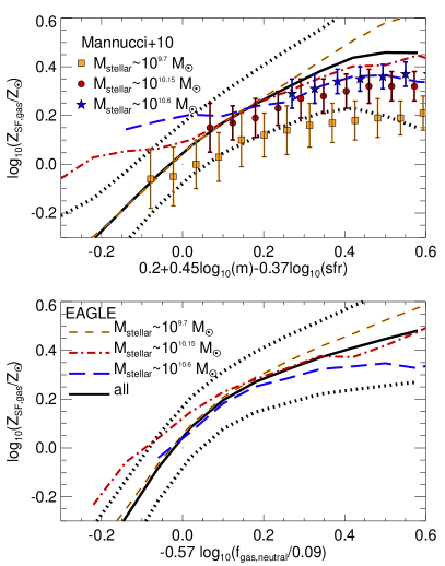
Figure 9: Top panel: Edge-on view of the plane of Eq. 10, comprised of star-forming gas metallicity, SFR and stellar mass in eagle. The thick solid line and the dotted lines show the median and 1$\sigma$ scatter, respectively, of all galaxies with $M_{\rm stellar}>10^{9}\,\rm M_{\odot}$ and SFR$>0.01\,\rm M_{\odot}\,yr^{-1}$. We also show the results for eagle galaxies in narrow bins of stellar masses in lines as labelled in the bottom panel. Observations at $z=0$ from Mannucci et al. (2010) are shown for the same $3$ bins of stellar mass we used for eagle. Observations are shown as symbols (labelled at the top-left corner). eagle galaxies with $M_{\rm stellar}>10^{10}\,\rm M_{\odot}$ and the observations agree to within $0.15$ dex, while lower-mass galaxies show discrepancies with the observations (up to $\approx 0.4$ dex). To convert the observations of Mannucci et al. from oxygen abundance to metallicity, we adopted a solar oxygen abundance of $12+\rm log_{10}(O/H)_{\odot}=8.69$ and $Z_{\odot}=0.0127$. Bottom panel: As in the top panel, but here we show an edge-on view of the relation between star-forming gas metallicity and neutral gas fraction (Eq. 9).

We assess the performance of the fits of Eqs. 9 and 10 and compare with the observations of Mannucci et al. (2010) in Fig. 9. In eagle, deviations from Eqs. 10 and 9 are seen at $Z_{\rm SF,gas}\gtrsim 3\,Z_{\odot}$ and $Z_{\rm SF,gas}\lesssim 0.7\,Z_{\odot}$. However, $73$% of the galaxies at $0\leq z\leq 4.5$ have $0.7\,Z_{\odot}\leq Z_{\rm SF,gas}\leq 3\,Z_{\odot}$, and thus the fits of Eqs. 9 and 10 are good descriptions of the majority of the galaxies in eagle. We also show how observed galaxies populate the plane of Eq. 10. For this we took the tabulated results for the dependence of gas metallicity on SFR and stellar mass from Mannucci et al. (2010) and show here $4$ bins of stellar mass. We find that observed galaxies follow a plane in the 3-dimensional space of metallicity, SFR and stellar mass that is very similar to the one that eagle galaxies follow. The agreement between observations and eagle galaxies with $M_{\rm stellar}\gtrsim 10^{10}\,\rm M_{\odot}$ is good (deviations are of $\lesssim 0.15$ dex). However, galaxies with $M_{\rm stellar}<10^{10}\,\rm M_{\odot}$ in the observations have metallicities that are $\approx 0.3-0.4$ dex lower than eagle galaxies of the same stellar mass. This is consistent with the discrepancies seen in the comparison presented in S15 between the predicted MZ relation in eagle and the observations of Tremonti et al. (2004). S15 show that this is related to the resolution of the simulation, as the higher resolution run that is recalibrated to reach a similar level of agreement with the $z=0.1$ stellar mass function and size-stellar mass relation, displays a MZ relation in much better agreement than the simulation we use here. The effect this discrepancy has on the results presented in Fig. 9 is minimal because the fit of Eq. 10 was calculated using the inverse of the number density as weight, and therefore low-mass galaxies, which display the largest discrepancies with the observed metallicity of galaxies, do not significantly skew the fit.

5 Conclusions

We have studied the evolution of the gas fraction and the multi-dimensional dependence between stellar mass, star formation rate, gas fraction and gas metallicity in the EAGLE suite of hydrodynamical simulations. We use the gas phase transitions from ionised to neutral, and from neutral to molecular, implemented on a particle-by-particle bases in post-processing by Lagos et al. (2015). The post-processing is done using the fitting functions of Rahmati et al. (2013a) for the transition from ionised to neutral gas, and of Gnedin & Kravtsov (2011) for the transition from neutral to molecular gas.

We summarise our main results below:

• We find that at fixed stellar mass, both the neutral and molecular gas fractions increase with redshift. In the case of the neutral gas fraction, this increase is a factor of $\approx 5$ between $z=0$ and $\approx 2.5$, while the same increase is seen in the molecular gas fraction over a shorter timescale, from $z=0$ to $z\approx 1.5$. The gas fractions at higher redshifts plateaus or even decreases. The specific SFR on the other hand increases by a factor of $\approx 15$ over the same redshift interval. The difference is due to high-$z$ galaxies having higher $\rm SFR/M_{\rm H_{2}}$ and $\rm SFR/M_{\rm neutral}$ than $z=0$ galaxies, which in turn is caused by the superlinear star formation law adopted in eagle and the higher gas pressure at high redshift.

• The evolution of the gas fraction is related to that of the SFR and the stellar mass. Galaxies show little evolution in their gas fraction at fixed stellar mass and SFR. This is a consequence of galaxies in eagle following with little scatter a 2-dimensional surface in the 3-dimensional space of stellar mass, SFR and neutral (or molecular) gas fraction. We term the plane tangential to this surface at the mean location of galaxies the “fundamental plane of star formation”, and provide fits derived from eaglein Eqs.6 and 7. These 2-dimensional surfaces are also seen in a compilation of observations of galaxies at $0\leq z\leq 3$ that we presented here. Observed and simulated galaxies populate the three-dimensional space of SFR, stellar mass and gas fractions in a very similar manner. A PCA analysis reveals that the relation between the neutral gas fraction, stellar mass and SFR contains most of the variance ($55$%) seen in the galaxy population of eagle, and therefore is one of the most fundamental correlations, which we term the “fundamental plane of star formation”.

• We attribute the existence of the 2-dimensional surfaces above to the self-regulation of star formation in galaxies: SFR is set by the balance between the accretion and outflow of gas. We suggest that the curvature of the plane in eagleis set by the model of star formation adopted, and affected by the relation between the ISM pressure and the SFR in eagle. We base these arguments on the analysis of how the plane changes when we change the SNe and AGN feedback strength, the equation of state imposed on the unresolved ISM and the power-law index in the star formation law adopted in eagle(Appendix C).

• The positions of galaxies in the 2-dimensional surface in the space of gas fraction, SFR and stellar mass are very well correlated with gas metallicity. The metallicity of the star-forming gas can therefore be predicted from the stellar masses and SFRs of galaxies, or from the neutral gas fraction of galaxies alone, to within $\approx 40$%. This relation between metallicity, stellar mass, SFR and neutral gas fraction appears in the PCA in the second component, and contributes $24$% to the variance seen in the galaxy population in eagle.

• The neutral gas fraction is more strongly correlated with the scatter in the stellar mass-metallicity (MZ) relation than the molecular gas fraction. Upcoming surveys will be able to test these predictions, as they will increase the number of galaxies sampled in their HI content by a factor of $\approx 100$ (see for instance the accepted proposals of the ASKAP HI All-Sky Survey , WALLABY, and the Deep Investigation of Neutral Gas Origins survey, DINGO, Johnston et al. 2008). Similarly, the Atacama Large Millimeter Array (ALMA) and the NOrthern Extended Millimeter Array (NOEMA) will be able to carry out a similar task but for H₂ in galaxies.

This is the first time it has been shown in simulations and a large compilation of observations that the stellar mass, SFR and gas fraction (either neutral or molecular) of galaxies follow a well-defined surface in the 3-dimensional space of stellar mass, SFR and neutral (or molecular) gas fraction. The fidelity to which eagle predictions describe the observations is remarkable, particularly since we focused on galaxy properties that were not used to constrain any of the free parameters in the sub-grid models.

Appendix A Strong and weak convergence tests

Table 3: eagle simulations used in this Appendix. The columns list: (1) the name of the simulation, (2) comoving box size, (3) number of particles, (4) initial particle masses of gas and (5) dark matter, (6) comoving gravitational softening length, and (7) maximum proper comoving Plummer-equivalent gravitational softening length. Units are indicated below the name of column. eagle adopts (6) as the softening length at $z\geq 2.8$, and (7) at $z<2.8$. The simulation Recal-L025N0752 has the same masses of particles and softening length values than the simulation Ref-L025N0752.

(1)	(2)	(3)	(4)	(5)	(6)	(7)
Name	$L$	# particles	gas particle mass	DM particle mass	Softening length	max. gravitational softening
Units	$[\rm cMpc]$		$[\rm M_{\odot}]$	$[\rm M_{\odot}]$	$[\rm ckpc]$	$[\rm pkpc]$
Ref-L025N0376	$25$	$2\times 376^{3}$	$1.81\times 10^{6}$	$9.7\times 10^{6}$	$2.66$	$0.7$
Ref-L025N0752	$25$	$2\times 752^{3}$	$2.26\times 10^{5}$	$1.21\times 10^{6}$	$1.33$	$0.35$

S15 introduced the concept of ‘strong’ and ‘weak’ convergence tests. Strong convergence refers to the case where a simulation is re-run with higher resolution (i.e. better mass and spatial resolution) adopting exactly the same subgrid physics and parameters. Weak convergence refers to the case when a simulation is re-run with higher resolution but the subgrid parameters are recalibrated to recover, as far as possible, similar agreement with the adopted calibration diagnostic (in the case of eagle, the $z=0.1$ galaxy stellar mass function and disk sizes of galaxies).

S15 introduced two higher-resolution versions of eagle, both in a box of ($25$ cMpc)³ and with $2\times 752^{3}$ particles, Ref-L025N0752 and Recal-L025N0752 (Table 3 shows some details of these simulations). These simulations have better spatial and mass resolution than the intermediate-resolution simulations by factors of $2$ and $8$, respectively. In the case of Ref-L025N0752, the parameters of the sub-grid physics are kept fixed (and therefore comparing with this simulation is a strong convergence test), while the simulation Recal-L025N0752 has $4$ parameters whose values have been slightly modified with respect to the reference simulation (and therefore comparing with this simulation is a weak convergence test).

Here we compare the results presented throughout the paper obtained using the Ref-L100N1504 simulation with the results of the higher-resolution simulations Ref-L025N0752 and Recal-L025N0752.

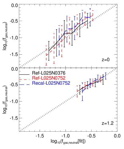
Figure 10: Strong and weak convergence tests. Top panel: The neutral gas fraction of galaxies, defined as in Eq. 3, in the simulations Ref-L025N0376, Ref-L025N0752 and Recal-L025N0752 at $z=0$, as a function of the neutral gas fraction calculated from the stellar masses and SFRs of galaxies by applying Eq. 6. We include all galaxies with $M_{\rm stellar}>10^{9}\,\rm M_{\odot}$. Lines with error bars show the medians and the $16^{\rm th}$ and $84^{\rm th}$ percentiles, respectively. The dotted line shows the relation $f_{\rm gas,neutral}\equiv f_{\rm neutral,fit}$. Bottom panel: As in the top panel but at $z=1.2$.

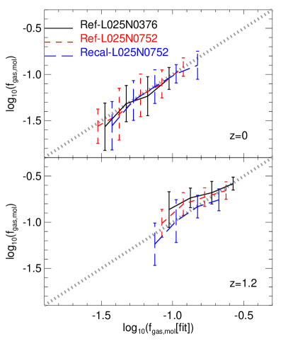
Figure 11: As in Fig. 10 but for the molecular gas fraction, defined as in Eq. 4. We use Eq. 7 to calculate the molecular gas fraction from the stellar masses and SFRs of galaxies.

Fig. 10 shows the neutral gas fraction as a function of the neutral gas fraction calculated from the stellar masses and SFRs of galaxies (i.e. applying Eq. 6). We show the relation for the simulations Ref-L025N0376, Ref-L025N0752 and Recal-L025N0752 at $z=0$ and $z=1.2$. We find that Ref-L025N0376 follows the same relation as Ref-L100N1504, showing that the box size has no effect on the results. The higher-resolution runs are very similar, both in terms of the median and the scatter of the relation. Deviations of the high resolution runs from the Ref-L025N0376 simulation are of $\lesssim 0.2$ dex at $z=0$ and of $\lesssim 0.1$ dex at $z=1.2$, with the largest values corresponding to galaxies with $f_{\rm gas,neutral}\gtrsim 0.25$.

In the case of the molecular gas fraction (Fig. 11), we find that deviations of the high resolution runs from the Ref-L025N0376 simulations are $\lesssim 0.1$ dex at $z=0$ and $\lesssim 0.25$ dex at $z=1.2$. The scatter of the relations does not vary with resolution. Galaxies showing the largest variations with resolution are those that have $f_{\rm gas,mol}\lesssim 0.1$ at $z\gtrsim 1$ that populate the turnover of the relation between molecular fraction, stellar mass and SFR. Interestingly, we find that Recal-L025N0752 deviates more from Ref-L025N0376 than Ref-L025N0752 in the metrics used here. This is due to gas metallicities in Recal-L025N0752 being on average a factor of $\approx 2$ lower than the gas metallicities in Ref-L025N0376 and Ref-L025N0752 (see S15 for details). This influences the density threshold for star formation and explicitly enters in the second principal component of $\S$ 4.1.

We conclude that there is good convergence of the results for the gas fractions with the numerical resolution.

Appendix B Principal Component Analysis

Here we perform three principal component analyses over stellar mass, SFR, metallicity of the star-forming gas and HI, H₂ or total neutral gas mass. We do this with the aim of studying how much the variance contained in the first and second principal components change if only one gas phase mass is included. If the “fundamental plane of star formation of galaxies” is indeed responsible for most of the variance seen in the galaxy population, we should find stellar mass, SFR and neutral gas mass in the first principal component, and being responsible for the largest variance compared to principal component vectors we obtain if we were to use atomic or molecular gas masses instead.

Table 4: PCA of galaxies in the Ref-L100N1504 simulation. Galaxies with $M_{\rm stellar}>10^{9}\,\rm M_{\odot}$, $\rm SFR<0.01\,M_{\odot}\,yr^{-1}$ and $M_{\rm H_{2}}/(M_{\rm H_{2}}+M_{\rm stellar})>0.01$ and in the redshift range $0\leq z\leq 4.5$ were included in the analysis. The PCA was conducted with the variables stellar mass, SFR, metallicity of the star-forming gas and HI, H₂ or total neutral gas mass. Here we show the first two principal components for each PCA together with the variance they are responsible for.

(1)	(2)	(3)	(4)	(5)	(6)
vector		$\hat{\rm x}_{1}$	$\hat{\rm x}_{2}$	$\hat{\rm x}_{3}$	$\hat{\rm x}_{4}$
Property	variance	$\frac{M_{\rm stellar}}{\rm M_{\odot}}$	$\rm\frac{SFR}{M_{\odot}\,yr^{-1}}$	$\rm\frac{Z_{\rm SF,gas}}{Z_{\odot}}$	$\frac{M_{\rm H_{2}}}{\rm M_{\odot}}$
PC1	$59$%	$0.49$	$0.5$	$0.58$	$0.4$
PC2	$35$%	$0.59$	$-0.24$	$0.21$	$-0.74$
Property		$\frac{M_{\rm stellar}}{\rm M_{\odot}}$	$\rm\frac{SFR}{M_{\odot}\,yr^{-1}}$	$\rm\frac{Z_{\rm SF,gas}}{Z_{\odot}}$	$\frac{M_{\rm HI}}{\rm M_{\odot}}$
PC1	$58$%	$0.28$	$0.76$	$0.06$	$-0.59$
PC2	$34$%	$0.6$	$0.18$	$-0.63$	$0.45$
Property		$\frac{M_{\rm stellar}}{\rm M_{\odot}}$	$\rm\frac{SFR}{M_{\odot}\,yr^{-1}}$	$\rm\frac{Z_{\rm SF,gas}}{Z_{\odot}}$	$\frac{M_{\rm neutral}}{\rm M_{\odot}}$
PC1	$61$%	$0.36$	$0.69$	$0.05$	$-0.62$
PC2	$34$%	$0.62$	$0.03$	$-0.71$	$0.34$

The three PCA are shown in Table 4. In the first PCA (which uses $M_{\rm H_{2}}$), the first principal component (PC1) has a strong contribution from the gas metallicity, which we do not see in PC1 when $M_{\rm HI}$ or $M_{\rm neutral}$ are used instead of $M_{\rm H_{2}}$. We see that PC1 in the case $M_{\rm neutral}$ is used has the largest variance, which is what we expected if the fundamental plane of star formation introduced in $\S$ 4.2 was indeed responsible for most of the variance seen in the galaxy population. This confirms the analysis presented in $\S$ 4. We again see that the metallcity of the star-forming gas has a large weight in the second principal component in the three case we analyse here.

Appendix C Effects of subgrid modelling on the fundamental plane of star formation

One of the main advantages of the eagle hydrodynamical simulation suite is that it includes a series of runs in which the subgrid models and model parameters are varied, in addition to the reference run that we analysed in $\S$ $3$ and $4$. C15 introduced $9$ runs in which the parameters of the reference model are altered (see Table $1$ in C15). Here we show how the fundamental plane of star formation in eagle is affected by changes in the stellar and AGN feedback strength and model, in the polytropic index of the equation of state applied to gas particles that have temperatures below an imposed temperature floor, and in the power-law index adopted in the star formation law (see $\S$ 2.1 for details). We use the models of Table 5 to study how the relation between neutral gas fraction, SFR and stellar mass changes under changes in the parameters of the subgrid physics.

Table 5: Variations of the reference model studied here. These variations were run in the L025N0376 setup (a simulation in a cubic volume of length $25$ cMpc on a side, using $376^{3}$ particles of dark matter and an equal number of baryonic particles; see Table 3 for more details). The reference model has the following parameter values: $f_{\rm th,max}=3.0$, $f_{\rm th,min}=0.3$ (govern the stellar feedback strength), $\rm log_{10}(\Delta T_{\rm AGN}/K)=8.5$ (governs the AGN feedback strength), $\gamma_{\rm eos}=4/3$ (governs the relation between pressure and density for gas particles with temperatures below $T_{\rm eos}=8\times 10^{3}$ K), and a power-law dependence in the star formation law of $n=1.4$. In the bottom two models, the scaling of $f_{\rm th}$ is changed to depend on the velocity dispersion of the DM (FB$\sigma$) and on the gas metallicity alone (FBZ). In the reference model, $f_{\rm th}$ depends on gas metallicity and density. See $\S$ 2.1 for a description of the subgrid models and more details on the parameters included in eagle.

(1)	(2)
Model	Parameters changed
WeakFB	$f_{\rm th,max}=1.5$, $f_{\rm th,min}=0.15$
StrongFB	$f_{\rm th,max}=6$,   $f_{\rm th,min}=0.6$
AGNTd8	$\rm log_{10}(\Delta T_{\rm AGN}/K)=8$
AGNTd9	$\rm log_{10}(\Delta T_{\rm AGN}/K)=9$
eos1	$\gamma_{\rm eos}=1$
eos5$/$3	$\gamma_{\rm eos}=5/3$
KSNormHi	$n=4.8$
KSNormLow	$n=0.48$
Model	$f_{\rm th}$-scaling
FB$\sigma$	$\sigma^{2}_{\rm DM}$
FBZ	$Z_{\rm SF,gas}$

Figure 12: An edge-on view of the plane of neutral gas fraction, stellar mass and SFR, as defined in Eq. 6. Here we include galaxies in all the simulations that have $M_{\rm stellar}>10^{9}\,\rm M_{\odot}$ and that are in the redshift range $0\leq z\leq 4.5$. The results for the simulation Ref-L025N0376 are shown in each panel, while the results of the simulations WeakFB, StrongFB are shown in the top panel, FBZ and FB$\sigma$ in the next-to-top panel, AGNTd8 and AGNTd9 in the middle panel, eos1 and eos5$/$3 in the next-to-bottom panel, and KSNormHi and KSNormLow in the bottom panel, as labelled in each panel. Lines with error bars show the medians and $16^{\rm th}$ to $84^{\rm th}$ percentiles for each model, respectively. All variations of the reference model were run in the L025N0376 setup.

We find that changing the strength of stellar feedback (WeakFB and StrongFB; top panel in Fig. 12) has a mild effect on the normalisation of the fundamental plane of star formation. Weaker feedback produces higher neutral gas fractions at fixed stellar mass and SFR with respect to the reference model (and the opposite is true for stronger feedback). Under self-regulation of star formation, weaker feedback would produce lower outflow rates, which in turn produces higher gas fraction and SFRs compared to stronger feedback. Note that the median relations in the models with weak/strong stellar feedback are almost parallel to each other which supports our interpretation that the curvature of the fundamental plane of star formation is set by the physics of star formation (i.e. how the gas gets converted into stars), while the normalisation is set by the self-regulation of star formation. The effect of the self-regulation is suggested by the change in the scatter of the fundamental plane when different feedback strength are adopted. A weaker feedback produces larger scatter, consistent with the less efficient self-regulation. A change in the scatter is also seen if we change the model of stellar feedback (FBZ and FB$\sigma$ models), where both lead to an increase in the scatter, due to the change in the timescale of self-regulation. Regarding the curvature, we see that changing the index in the equation of state imposed on the unresolved ISM, $\gamma_{\rm eos}$ (next-to-bottom panel in Fig. 12), does not change the normalisation of the fundamental plane of star formation, but changes the slope. For example, model eos5$/$3 produces a slightly steeper relation compared to the reference model and the model eos1 at $\rm log_{10}(f_{\rm gas,neutral}/0.046)\gtrsim 0.5$. Effectively, changing the index in the equation of state has the effect of slightly changing the curvature of the fundamental plane of star formation while not changing the normalisation significantly. The effect on the curvature of the fundamental plane of star formation by how star formation is modelled in eagle becomes more apparent in the bottom panel of Fig. 12) where we varied the power-law index in the star formation law, $n$. A lower $n$ produces a much flatter plane than in reference model, while increasing $n$ steepens the plane.

Changing the AGN feedback strength has little effect on the fundamental plane of star formation, pointing to stellar feedback being the main mechanism driving outflows in star-forming galaxies.

In short, feedback from star formation (or AGN) produces an effective amount of feedback to balance the cosmological gas accretion rate, and the star formation recipe determines the rate at which gas gets converted into stars. These two ‘rules’ help us understanding what we see in Fig. 12 (see Haas et al. 2013a and Haas et al. 2013b for detailed studied of the self-regulation of star formation in galaxies).

References

- Baes et al. (2011) Baes M., Verstappen J., De Looze I., Fritz J., Saftly W., Vidal Pérez E., Stalevski M., Valcke S., 2011, ApJS, 196, 22
- Bahé et al. (2016) Bahé Y. M., Crain R. A., Kauffmann G., Bower R. G., Schaye J., Furlong M., Lagos C., Schaller M. et al, 2016, MNRAS, 456, 1115
- Benson & Bower (2010) Benson A. J., Bower R., 2010, MNRAS, 405, 1573
- Bolatto et al. (2013) Bolatto A. D., Wolfire M., Leroy A. K., 2013, ARA&A, 51, 207
- Booth & Schaye (2010) Booth C. M., Schaye J., 2010, MNRAS, 405, L1
- Boselli et al. (2014a) Boselli A., Cortese L., Boquien M., 2014a, A&A, 564, A65
- Boselli et al. (2014b) Boselli A., Cortese L., Boquien M., Boissier S., Catinella B., Lagos C., Saintonge A., 2014b, A&A, 564, A66
- Bothwell et al. (2013) Bothwell M. S., Maiolino R., Kennicutt R., Cresci G., Mannucci F., Marconi A., Cicone C., 2013, MNRAS, 433, 1425
- Bothwell et al. (2015) Bothwell M. S., Maiolino R., Peng Y., Cicone C., Griffith H., Wagg J., 2015, ArXiv:1507.01004
- Bothwell et al. (2014) Bothwell M. S., Wagg J., Cicone C., Maiolino R., Møller P., Aravena M., De Breuck C., Peng Y. et al, 2014, MNRAS, 445, 2599
- Brinchmann et al. (2004) Brinchmann J., Charlot S., White S. D. M., Tremonti C., Kauffmann G., Heckman T., Brinkmann J., 2004, MNRAS, 351, 1151
- Brown et al. (2015) Brown T., Catinella B., Cortese L., Kilborn V., Haynes M. P., Giovanelli R., 2015, MNRAS, 452, 2479
- Cappellari et al. (2011) Cappellari M., Emsellem E., Krajnović D., McDermid R. M., Scott N., Verdoes Kleijn G. A., Young L. M., Alatalo K. et al, 2011, MNRAS, 413, 813
- Cappellari et al. (2013) Cappellari M., McDermid R. M., Alatalo K., Blitz L., Bois M., Bournaud F., Bureau M., Crocker A. F. et al, 2013, MNRAS, 432, 1862
- Catinella et al. (2010) Catinella B., Schiminovich D., Kauffmann G., Fabello S., Wang J., Hummels C., Lemonias J., Moran S. M. et al, 2010, MNRAS, 403, 683
- Chabrier (2003) Chabrier G., 2003, PASP, 115, 763
- Crain et al. (2015) Crain R. A., Schaye J., Bower R. G., Furlong M., Schaller M., Theuns T., Dalla Vecchia C., Frenk C. S. et al, 2015, MNRAS, 450, 1937
- Daddi et al. (2007) Daddi E., Dickinson M., Morrison G., Chary R., Cimatti A., Elbaz D., Frayer D., Renzini A. et al, 2007, ApJ, 670, 156
- Dalla Vecchia & Schaye (2012) Dalla Vecchia C., Schaye J., 2012, MNRAS, 426, 140
- Damen et al. (2009) Damen M., Labbé I., Franx M., van Dokkum P. G., Taylor E. N., Gawiser E. J., 2009, ApJ, 690, 937
- Davé et al. (2012) Davé R., Finlator K., Oppenheimer B. D., 2012, MNRAS, 421, 98
- Davis et al. (2014) Davis T. A., Young L. M., Crocker A. F., Bureau M., Blitz L., Alatalo K., Emsellem E., Naab T. et al, 2014, MNRAS, 444, 3427
- De Rossi et al. (2015) De Rossi M. E., Theuns T., Font A. S., McCarthy I. G., 2015, MNRAS, 452, 486
- Dessauges-Zavadsky et al. (2015) Dessauges-Zavadsky M., Zamojski M., Schaerer D., Combes F., Egami E., Swinbank A. M., Richard J., Sklias P. et al, 2015, A&A, 577, A50
- Doi et al. (2010) Doi M., Tanaka M., Fukugita M., Gunn J. E., Yasuda N., Ivezić Ž., Brinkmann J., de Haars E. et al, 2010, AJ, 139, 1628
- Dolag et al. (2009) Dolag K., Borgani S., Murante G., Springel V., 2009, MNRAS, 399, 497
- Dwek (1998) Dwek E., 1998, ApJ, 501, 643
- Furlong et al. (2015a) Furlong M., Bower R. G., Crain R. A., Schaye J., Theuns T., Trayford J. W., Qu Y., Schaller M. et al, 2015a, ArXiv:1510.05645
- Furlong et al. (2015b) Furlong M., Bower R. G., Theuns T., Schaye J., Crain R. A., Schaller M., Dalla Vecchia C., Frenk C. S. et al, 2015b, MNRAS, 450, 4486
- Geach et al. (2011) Geach J. E., Smail I., Moran S. M., MacArthur L. A., Lagos C. d. P., Edge A. C., 2011, ApJ, 730, L19+
- Giovanelli et al. (2005) Giovanelli R., Haynes M. P., Kent B. R., Perillat P., Saintonge A., Brosch N., Catinella B., Hoffman G. L. et al, 2005, AJ, 130, 2598
- Gnedin & Draine (2014) Gnedin N. Y., Draine B. T., 2014, ApJ, 795, 37
- Gnedin & Kravtsov (2011) Gnedin N. Y., Kravtsov A. V., 2011, ApJ, 728, 88
- Haardt & Madau (2001) Haardt F., Madau P., 2001, in Clusters of Galaxies and the High Redshift Universe Observed in X-rays, Neumann D. M., Tran J. T. V., eds., p. 64
- Haas et al. (2013a) Haas M. R., Schaye J., Booth C. M., Dalla Vecchia C., Springel V., Theuns T., Wiersma R. P. C., 2013a, MNRAS, 435, 2931
- Haas et al. (2013b) —, 2013b, MNRAS, 435, 2955
- Haynes et al. (2011) Haynes M. P., Giovanelli R., Martin A. M., Hess K. M., Saintonge A., Adams E. A. K., Hallenbeck G., Hoffman G. L. et al, 2011, AJ, 142, 170
- Herrera-Camus et al. (2012) Herrera-Camus R., Fisher D. B., Bolatto A. D., Leroy A. K., Walter F., Gordon K. D., Roman-Duval J., Donaldson J. et al, 2012, ApJ, 752, 112
- Hughes et al. (2013) Hughes T. M., Cortese L., Boselli A., Gavazzi G., Davies J. I., 2013, A&A, 550, A115
- Johnston et al. (2008) Johnston S., Taylor R., Bailes M., Bartel N., Baugh C., Bietenholz M., Blake C., Braun R. et al, 2008, Experimental Astronomy, 22, 151
- Kennicutt (1998) Kennicutt Jr. R. C., 1998, ApJ, 498, 541
- Krumholz (2013) Krumholz M. R., 2013, MNRAS, 436, 2747
- Lagos et al. (2015) Lagos C. d. P., Crain R. A., Schaye J., Furlong M., Frenk C. S., Bower R. G., Schaller M., Theuns T. et al, 2015, MNRAS, 452, 3815
- Lagos et al. (2011) Lagos C. D. P., Lacey C. G., Baugh C. M., Bower R. G., Benson A. J., 2011, MNRAS, 416, 1566
- Lara-López et al. (2010) Lara-López M. A., Cepa J., Bongiovanni A., Pérez García A. M., Ederoclite A., Castañeda H., Fernández Lorenzo M., Pović M. et al, 2010, A&A, 521, L53
- Lara-López et al. (2013) Lara-López M. A., Hopkins A. M., López-Sánchez A. R., Brough S., Colless M., Bland-Hawthorn J., Driver S., Foster C. et al, 2013, MNRAS, 433, L35
- Mannucci et al. (2010) Mannucci F., Cresci G., Maiolino R., Marconi A., Gnerucci A., 2010, MNRAS, 408, 2115
- Marigo (2001) Marigo P., 2001, A&A, 370, 194
- McAlpine et al. (2015) McAlpine S., Helly J. C., Schaller M., Trayford J. W., Qu Y., Furlong M., Bower R. G., Crain R. A. et al, 2015, ArXiv:1510.01320
- Meyer et al. (2004) Meyer M. J., Zwaan M. A., Webster R. L., Staveley-Smith L., Ryan-Weber E., Drinkwater M. J., Barnes D. G., Howlett M. et al, 2004, MNRAS, 350, 1195
- Noeske et al. (2007) Noeske K. G., Weiner B. J., Faber S. M., Papovich C., Koo D. C., Somerville R. S., Bundy K., Conselice C. J. et al, 2007, ApJ, 660, L43
- Pawlik & Schaye (2008) Pawlik A. H., Schaye J., 2008, MNRAS, 389, 651
- Planck Collaboration (2014) Planck Collaboration, 2014, A&A, 571, A16
- Portinari et al. (1998) Portinari L., Chiosi C., Bressan A., 1998, A&A, 334, 505
- Rahmati et al. (2013a) Rahmati A., Pawlik A. H., Raicevic M., Schaye J., 2013a, MNRAS, 430, 2427
- Rahmati et al. (2013b) Rahmati A., Schaye J., Pawlik A. H., Raicevic M., 2013b, MNRAS, 431, 2261
- Richings et al. (2014) Richings A. J., Schaye J., Oppenheimer B. D., 2014, MNRAS, 442, 2780
- Robotham & Obreschkow (2015) Robotham A. S. G., Obreschkow D., 2015, ArXiv:1508.02145
- Rodighiero et al. (2010) Rodighiero G., Cimatti A., Gruppioni C., Popesso P., Andreani P., Altieri B., Aussel H., Berta S. et al, 2010, A&A, 518, L25+
- Rosas-Guevara et al. (2015) Rosas-Guevara Y. M., Bower R. G., Schaye J., Furlong M., Frenk C. S., Booth C. M., Crain R. A., Dalla Vecchia C. et al, 2015, MNRAS, 454, 1038
- Saintonge et al. (2011) Saintonge A., Kauffmann G., Kramer C., Tacconi L. J., Buchbender C., Catinella B., Fabello S., Graciá-Carpio J. et al, 2011, MNRAS, 415, 32
- Saintonge et al. (2013) Saintonge A., Lutz D., Genzel R., Magnelli B., Nordon R., Tacconi L. J., Baker A. J., Bandara K. et al, 2013, ApJ, 778, 2
- Salim et al. (2015) Salim S., Lee J. C., Davé R., Dickinson M., 2015, ApJ, 808, 25
- Salim et al. (2014) Salim S., Lee J. C., Ly C., Brinchmann J., Davé R., Dickinson M., Salzer J. J., Charlot S., 2014, ApJ, 797, 126
- Santini et al. (2009) Santini P., Fontana A., Grazian A., Salimbeni S., Fiore F., Fontanot F., Boutsia K., Castellano M. et al, 2009, A&A, 504, 751
- Santini et al. (2014) Santini P., Maiolino R., Magnelli B., Lutz D., Lamastra A., Li Causi G., Eales S., Andreani P. et al, 2014, A&A, 562, A30
- Schaller et al. (2015) Schaller M., Dalla Vecchia C., Schaye J., Bower R. G., Theuns T., Crain R. A., Furlong M., McCarthy I. G., 2015, ArXiv:1509.05056
- Schaye (2001) Schaye J., 2001, ApJ, 562, L95
- Schaye (2004) —, 2004, ApJ, 609, 667
- Schaye et al. (2015) Schaye J., Crain R. A., Bower R. G., Furlong M., Schaller M., Theuns T., Dalla Vecchia C., Frenk C. S. et al, 2015, MNRAS, 446, 521
- Schaye & Dalla Vecchia (2008) Schaye J., Dalla Vecchia C., 2008, MNRAS, 383, 1210
- Schaye et al. (2010) Schaye J., Dalla Vecchia C., Booth C. M., Wiersma R. P. C., Theuns T., Haas M. R., Bertone S., Duffy A. R. et al, 2010, MNRAS, 402, 1536
- Serra et al. (2012) Serra P., Oosterloo T., Morganti R., Alatalo K., Blitz L., Bois M., Bournaud F., Bureau M. et al, 2012, MNRAS, 2823
- Sobral et al. (2014) Sobral D., Best P. N., Smail I., Mobasher B., Stott J., Nisbet D., 2014, MNRAS, 437, 3516
- Somerville & Davé (2015) Somerville R. S., Davé R., 2015, ARA&A, 53, 51
- Springel (2005) Springel V., 2005, MNRAS, 364, 1105
- Springel et al. (2008) Springel V., Wang J., Vogelsberger M., Ludlow A., Jenkins A., Helmi A., Navarro J. F., Frenk C. S. et al, 2008, MNRAS, 391, 1685
- Springel et al. (2001) Springel V., White S. D. M., Tormen G., Kauffmann G., 2001, MNRAS, 328, 726
- Springob et al. (2005) Springob C. M., Haynes M. P., Giovanelli R., Kent B. R., 2005, ApJS, 160, 149
- Tacconi et al. (2013) Tacconi L. J., Neri R., Genzel R., Combes F., Bolatto A., Cooper M. C., Wuyts S., Bournaud F. et al, 2013, ApJ, 768, 74
- Thielemann et al. (2003) Thielemann F.-K., Argast D., Brachwitz F., Hix W. R., Höflich P., Liebendörfer M., Martinez-Pinedo G., Mezzacappa A., Nomoto K., Panov I., 2003, in From Twilight to Highlight: The Physics of Supernovae, Hillebrandt W., Leibundgut B., eds., p. 331
- Trayford et al. (2015) Trayford J. W., Theuns T., Bower R. G., Schaye J., Furlong M., Schaller M., Frenk C. S., Crain R. A. et al, 2015, MNRAS, 452, 2879
- Tremonti et al. (2004) Tremonti C. A., Heckman T. M., Kauffmann G., Brinchmann J., Charlot S., White S. D. M., Seibert M., Peng E. W. et al, 2004, ApJ, 613, 898
- Wiersma et al. (2009a) Wiersma R. P. C., Schaye J., Smith B. D., 2009a, MNRAS, 393, 99
- Wiersma et al. (2009b) Wiersma R. P. C., Schaye J., Theuns T., Dalla Vecchia C., Tornatore L., 2009b, MNRAS, 399, 574
- Young et al. (2011) Young L. M., Bureau M., Davis T. A., Combes F., McDermid R. M., Alatalo K., Blitz L., Bois M. et al, 2011, MNRAS, 414, 940
- Zahid et al. (2014) Zahid H. J., Dima G. I., Kudritzki R.-P., Kewley L. J., Geller M. J., Hwang H. S., Silverman J. D., Kashino D., 2014, ApJ, 791, 130