Circulating persistent current and induced magnetic field in a fractal network

Abstract

We present the overall conductance as well as the circulating currents in individual loops of a Sierpinski gasket (SPG) as we apply bias voltage via the side attached electrodes. SPG being a self-similar structure, its manifestation on loop currents and magnetic fields are examined in various generations of this fractal and it has been observed that for a given configuration of the electrodes, the physical quantities exhibit certain regularity as we go from one generation to another. Also a notable feature is the introduction of anisotropy in hopping causes an increase in magnitude of overall transport current. These features are a subject of interest in this article.

I Introduction

Fractals aroused a lot of interest in the minds of physicists and mathematecians for several decades because of their amazing physical and geometrical properties. Diverse types of fractals are present in nature, and can also be generated by means of some recursive rules. Among them some are of deterministic type, lying between systems of perfect periodic order and completely random ones, making it easier to explain the basic features of fractals fick . Sierpinski Gasket (SPG) is one such deterministic self-similar fractal where every scaled version exactly resembles to the original one. With advancement of lithographic techniques experimental designing of such geometry has become tailor made new . Electron transport through SPG has become a topic of current research interest fr1 ; fr2 ; fr3 ; Maiti1 . Articles on quantum transport in mesoscopic systems mostly discuss the overall conduction properties orella1 ; tagami ; ventra2 ; ventra1 ; aviram ; nitzan1 ; skm1 ; woi , while little interests have been paid to distribution of currents at the various junctions and branches of a quantum network. Some articles brought into light, current distributions within the quantum networks by addressing possible interference effects arising from the multiple conduction pathways nishi ; suka . While examining current distributions in systems attached to electrodes, possibility of such currents giving rise to circular currents have been reported cir1 . But a proper definition of circular current came a little later cir3 . Like the persistent current in isolated mesoscopic ring as predicted by Büttiker Butti and his co-workers in $1983$, this circular current also persists as long as bias voltage is maintained. The behavior of persistent current in different geometries including fractals was usually explored only in presence of flux gefen ; Ore1 ; san1 ; san2 ; ambe ; schm1 ; schm2 , though the detail phenomena in individual loops of a quantum network need to be explored. Idea of persistent current arising as a direct consequence of Aharonov-Bohm (AB) effect led mesoscopic physics to the forefront of condensed matter physics. This self-sustaining current which originates in absence of external bias is a purely mesoscopic phenomenon and gets suppressed with increase in system size beyond the phase coherence length.

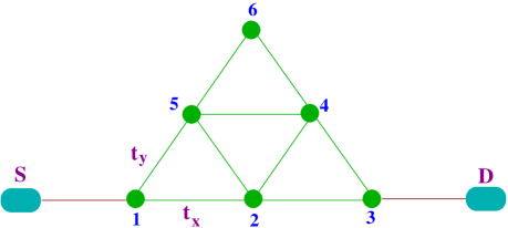
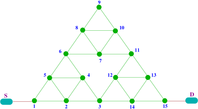
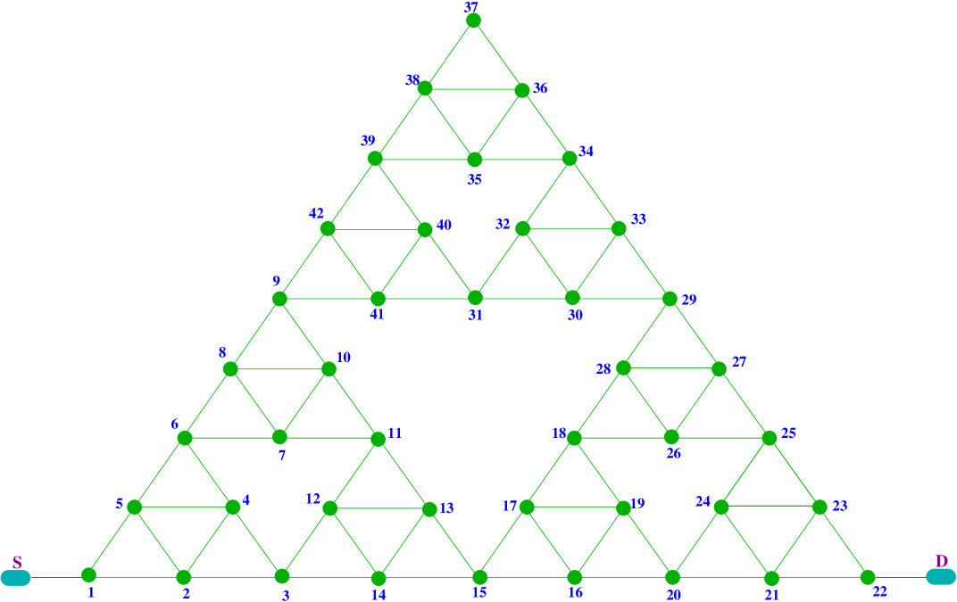
Figure 1: (Color online). $1$st, $2$nd and $3$rd generations (top to bottom) of a SPG fractal. Different numbers (viz, $1$, $2$, $3$, $\dots$) represent lattice sites of the network.

Some recent theoretical works have pointed out the fact that persistent current can be generated by circularly polarized light, twisted light and shaped photon pulses l1 ; l2 ; l3 ; l4 ; l5 ; l6 . This equilibrium current arises not only in isolated geometries but also appears in loops connected to external electrodes. Persistent current was observed experimentally in closed systems levy ; mailly ; chand , but experimental demonstration of its counterpart in open system has not been observed till now to the best of our knowledge. Persistent current in presence of bias voltage can be observed in loop structures only, where a loop is connected to external reservoirs. Another notable feature that came into limelight is the fact that this circular current in turn gives rise to a magnetic field at the center of the loop and this field can be utilized to design quantum devices cir3 . Orientation of a spin placed at the center of a loop geometry can be controlled by the magnetic field produced by circular current and this idea can be applied to generate spin based quantum devices. The following works dealt with some ways of controlling magnetic field externally. For example, Cho et al. Cho studied the behavior of coherent electron transport in a double quantum dot system and found that it acted as a magnetically polarized device due to quantum interference of electrons within the closed path of the device. They also showed that by varying the energy level of each dot, magnetic states of the device can be made up, down or non-polarized. In another work Lidar it has been depicted how an infinite array of parallel current carrying wires can produce exponentially localized magnetic field with peak value reaching upto $10\;$mT. A major drawback of this set-up is the issue of heating and loosing of coherence, and the device has been found to work well below the temperature $\ll 2.4\;$mK. In report by Pershin et al. Per , they showed how phase locked infra-red laser pulses can be used to generate local magnetic field at the ring center. Magnetic field of around $3\;$mT was induced at the center and it is quite comparable to that obtained in the preceding reference. In $2012$ Anda et al. Anda have provided the evidence of circular current in a ring with two quantum dots embedded in it and coupled to two electrodes, but nothing has been mentioned regarding the magnetic field induced by this current. In other recent work san3 it has been shown how the local magnetic field can be regulated in a conducting mesoscopic ring subjected to an in-plane electric field. Though few propositions have been made to scrutinize current distributions including circular current and associated magnetic field in different bridge systems, but most of these works are associated with simple loop geometries and no one has addressed these characteristics in any simple and/or complex network geometries. SPG fractal can be a suitable example of it which may exhibit interesting patterns by virtue of the self-similarity. The main fact presented in this paper is variation of currents and induced magnetic field in each triangle of a SPG network with applied voltage, and how the nature of circular current varies with generations. An interesting feature obtained from the model is the mirror symmetry of currents in each loop on either side of an imaginary vertical line drawn perpendicular to the line connecting the leads for the positions as given in Fig. 1 for any generation. We also present how the change in position of such leads affect circular currents and induced magnetic field. Our analysis can be useful to extract important information in other related self-similar structures.

The paper is arranged as follows. Section II gives the theoretical formulation with the numerical results discussed in subsequent Section III, which include the analysis of transmission spectra and transport current, hence follows the discussion of circular currents in individual loops and the associated magnetic fields. Finally, we conclude in the last Section IV.

II Model and Theoretical Formulation

We begin by referring to Fig. 1 depicting different generations of a SPG network connected to source ($S$) and drain ($D$) electrodes with the hopping in angular and horizontal directions denoted by $t_{x}$ and $t_{y}$, respectively. The filled green circles represent atomic sites and we describe the entire system by using a tight-binding formalism. The Hamiltonian of the entire system reads,

$$\mathcal{H}=H_{S}+H_{D}+H_{SPG}+H_{S,SPG}+H_{D,SPG}$$ (1)

First two terms correspond to the Hamiltonians for semi-infinite leads and can be expressed as

$$H_{S}+H_{D}=\sum\limits_{S,D}\left\{\sum\limits_{n}\epsilon_{0}\alpha_{n}^{\dagger}\alpha_{n}+\sum\limits_{n}t_{0}[\alpha_{n+1}^{\dagger}\alpha_{n}+h.c.]\right\}$$ (2)

where $\epsilon_{0}$ is the on-site energy and $t_{0}$ represents nearest-neighbor hopping strength in electrodes. Creation and annihilation operators for an electron in the $n$th site are labeled by $\alpha_{n}^{\dagger}$ and $\alpha_{n}$, respectively.

The Hamiltonian for the SPG triangle is

$$H_{SPG}=\sum\limits_{i}\epsilon_{i}c_{i}^{\dagger}c_{i}+\sum\limits_{\langle ij\rangle}t_{ij}\left[c_{i}^{\dagger}c_{j}+h.c.\right]$$ (3)

where $c_{i}^{\dagger}$ and $c_{i}$ stand for the creation and annihilation operators, while $\epsilon_{i}$ and $t_{ij}$ are the on-site energy and nearest-neighbor hopping integral, respectively, for the SPG. We take $\epsilon_{i}=\epsilon$ and $t_{ij}=t_{x}$ or $t_{y}$ depending on whether electron is hopping in the horizontal or in angular direction as show in Fig. 1.

Finally, the last two terms arise due to the coupling between semi-infinite leads and atomic sites of SPG network and explicitly we can write

$$H_{S,SPG}+H_{D,SPG}=\tau_{S}[c_{1}^{\dagger}\alpha_{0}+h.c.]+\tau_{D}[c_{q}^{\dagger}\alpha_{n+1}+h.c.]$$ (4)

where, the source is coupled to site $1$ of the SPG via the hopping strength $\tau_{S}$ and the other lead is attached to site $q$, which is variable, through the hopping strength $\tau_{D}$.

II.1 Evaluation of transport current

In order to evaluate transport current due to flow of electrons from source to drain, we need to calculate two-terminal transmission probability $T(E)$. Using Green’s function formalism $T(E)$ can be obtained assuming the transport to be taking place in the coherent regime. Thus we can express the single particle Green’s function operator in the form defined by

$$G=(E-H+i\eta)^{-1}$$ (5)

Introducing the contact self energies $\Sigma_{S}$ and $\Sigma_{D}$ which incorporate the effect of couplings between (SPG) and the semi-infinite leads, the problem of determining $G^{r}$ in full Hilbert space can be transformed to the reduced Hilbert space spanned by the system itself, and we can write the effective Green’s function datta

$$\mathcal{G}^{r}=(E-H_{SPG}-\Sigma_{S}-\Sigma_{D})^{-1}$$ (6)

In terms of retarded and advanced Green’s functions, the two-terminal transmission probability of an electron can be written as datta

$$T(E)=Tr[\Gamma_{S}\mathcal{G}^{r}\Gamma_{D}\mathcal{G}^{a}]$$ (7)

where $\mathcal{G}^{a}=[\mathcal{G}^{r}]^{\dagger}$, $\Gamma_{S}$ and $\Gamma_{D}$ represent the coupling matrices.

This transmission function can be utilized to find junction current $I_{T}$ as a function of bias voltage following the relation datta

$$I_{T}=\frac{2e}{h}\int\limits_{-\infty}^{\infty}T(E)\left[f_{S}(E)-f_{D}(E)\right]\;dE$$ (8)

where, $f_{S}(E)$ and $f_{D}(E)$ are the Fermi functions of the source and drain, respectively. At absolute zero temperature this relation simplifies to

$$I=\frac{2e}{h}\int\limits_{E_{F}-eV/2}^{E_{F}+eV/2}T(E)\;dE$$ (9)

where, $E_{F}$ is the equilibrium Fermi energy and we set it to zero throughout the calculations.

II.2 Circular current and associated magnetic field

To determine circular current in each of the plaquettes of a SPG network, let us first analyze the current distribution in a circular loop as shown in Fig 2. The diagram shows that the current flowing in the electrodes being $I_{T}$, while $I_{1}$ and $I_{2}$ are currents passing through the upper and lower branches of the circular geometry. Net current can be expressed in terms of branch currents as

$$I_{T}=I_{1}-I_{2}$$ (10)

Here we have assumed clockwise direction of current to be positive. The above expression (Eq.10) can be rearranged in the form cir3 $I_{T}=(I_{1}-I_{c})-(I_{2}-I_{c})=I_{1}^{tr}-I_{2}^{tr}$, where $I_{c}$ is the current circulating in the ring, and being persistent in nature, arises solely due to the bias voltage.

This self-sustaining current can be expressed as

$$I_{c}=\frac{I_{1}L_{1}+I_{2}L_{2}}{L}$$ (11)

where, $L_{1}$ and $L_{2}$ are the lengths of the upper and lower arms and $L=L_{1}+L_{2}$. This current does not contribute to the net current, only

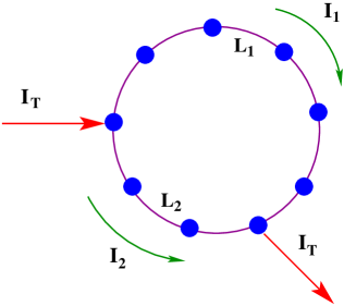
Figure 2: (Color online). Circular loop connected to two leads exhibiting currents in upper and lower arms of the ring.

keeps on circulating in the loop. The formula can be generalized in case of more than two branches as

$$I_{c}=\frac{\sum\limits_{i}{I_{i}L_{i}}}{L}$$ (12)

From the expressions of circular current it becomes clear that we need to evaluate the branch currents, which can be done using the Green’s function formalism. First we calculate the bond current density tag

$$J_{ij}=\frac{4e}{h}\mbox{Im}[(H_{SPG})_{ij}\mathcal{G}_{ij}^{n}]$$ (13)

We define $\mathcal{G}^{n}$ as the correlated Green’s function given by the formula

$$\mathcal{G}^{n}=\mathcal{G}^{r}\Gamma_{S}\mathcal{G}^{a}$$ (14)

where, each term has the same meaning as mentioned earlier. Now, the bond current between nearest-neighbor sites $i$ and $j$ at absolute zero temperature is given by

$$I_{ij}=\int\limits_{E_{F}-eV/2}^{E_{F}+eV/2}J_{ij}(E)\;dE$$ (15)

Substituting the above expression in Eq. 11 or Eq. 12 depending upon the system, we finally evaluate circular currents in each triangle of SPG network. This circulating current gives rise to local magnetic field at the center of each plaquette and it can be analyzed using Biot-Savart’s law cir3

$$B=\sum\limits_{ij}\frac{\mu_{0}}{4\pi}\int I_{ij}\frac{d\vec{r}\times(\vec{r}-\vec{r}^{\prime})}{|\vec{r}-\vec{r}^{\prime}|^{3}}$$ (16)

where, $\mu_{0}$ signifies the magnetic constant and $\vec{r^{\prime}}$ describes the position vector of the bond current element.

III Numerical Results and Discussion

Based on above theoretical formulation we present below the results of our numerical calculations.

III.1 Transmission spectra and transport current

Figure 3 shows the two-terminal transmission probability $T$ as

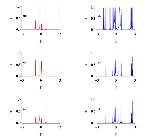
Figure 3: (Color online). $T$-$E$ characteristics for a $3$rd generation SPG ($N=42$), where the left and right columns correspond to $t_{x}=t_{y}=1\;$eV and $t_{x}=1.0\;$eV, $t_{y}=0.7\;$eV, respectively. Here the source is coupled to site $1$, while the drain is attached to three different sites $22$, $29$ and $9$ those are presented in the $1$st, $2$nd and $3$rd rows, respectively.

function of energy $E$ for a $3$rd generation SPG network. The three different rows correspond to three different positions of drain ($22$, $29$ and $9$) with source being kept fixed at position $1$. The left column corresponds to the case of isotropic hopping integral $t_{x}=t_{y}$, while the other column represents the anisotropic ($t_{x}\neq t_{y}$) counterpart. It is evident from the spectra that anisotropy introduces more peaks in the transmission characteristics, thereby making the system more conducting in nature than the isotropic case. It is also observed from the $T$-$E$ characteristics, that the conducting nature is highest for the first row (which is even more prominent in Fig. 3(b)) when leads are connected at two sides of the SPG, compared to other rows when drain lead is connected above the base line.

From this result (Fig. 3) we can make a sense about the nature of transport current and how anisotropy may result in an increase in magnitude of the current. The $I_{T}$-$V$ characteristics of the identical SPG fractal are shown in Fig. 4 for three different positions of the drain ($22$, $29$, and $9$), as taken in Fig. 3, connecting the source lead to the site $1$. The solid and dashed curves

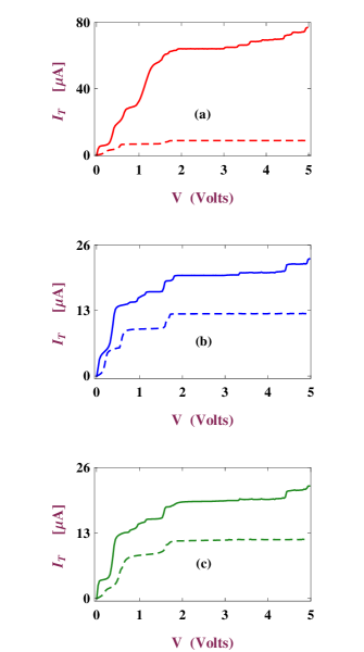
Figure 4: (Color online). $I_{T}$-$V$ characteristics of a $42$-site SPG network where the dotted and solid lines correspond to isotropic hopping ($t_{x}=t_{y}=1\;$eV) and its anisotropic counterpart ($t_{x}=1\;$eV, $t_{y}=0.7\;$eV). Here the source is coupled to site $1$, while the drain is attached to three different sites those are: (a) $22$, (b) $29$ and (c) $9$.

represent anisotropic and isotropic fractals respectively. These spectra clearly depict the increment of current for the anisotropic hopping case following the transmission characteristics as presented in Fig. 3. Physically anisotropy reduces

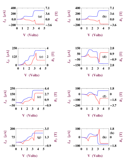
Figure 5: (Color online). Variation of circular current $I_{cn}$ ($n$ corresponds to individual triangles) and associated magnetic field $B_{n}$ with bias voltage for each plaquettes of 1st generation SPG network. Here the red curves are for $t_{x}=t_{y}=1\;$eV while blue lines are for $t_{x}=1\;$eV, $t_{y}=0.7\;$eV. For (a)-(d) leads are connected at $1$ and $3$ sites, while for (e)-(h) they are coupled to sites $1$ and $6$.

the possibility of destructive quantum interference in the various loops of the SPG network and hence increases the overall transport current. We also find that the junction current becomes maximum when leads are attached

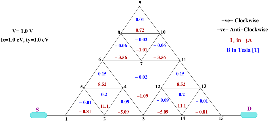
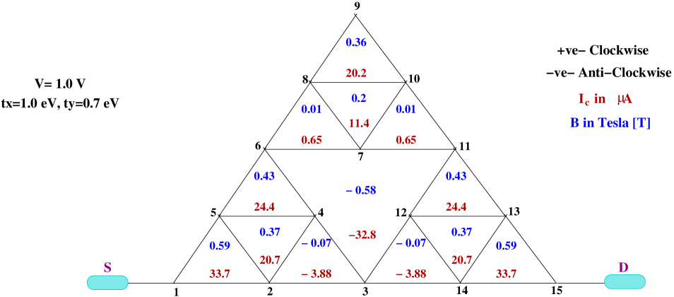
Figure 6: (Color online). Values of circular currents and associated magnetic fields at individual plaquettes of a $2$nd generation SPG ($N=15$) network. All the other physical parameters are clearly mentioned in the figure.

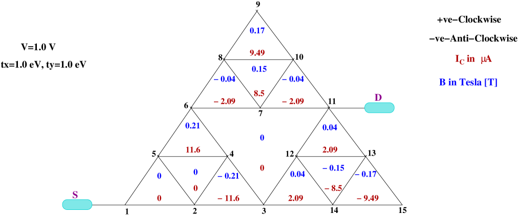
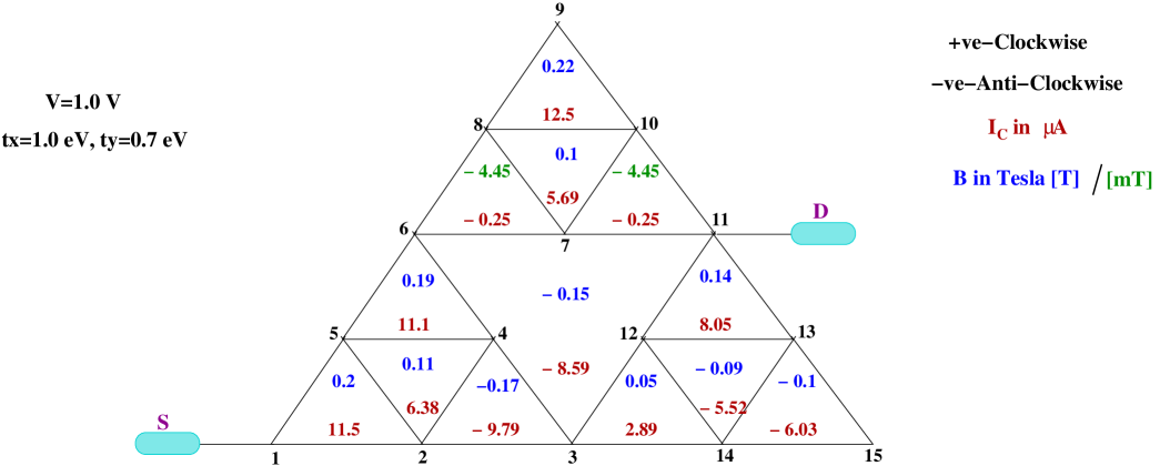
Figure 7: (Color online). Same as Fig. 6 with different source-SPG-drain configuration.

on two sides of the base of SPG. The reason behind it is that the chances of destructive interference is less for this SPG-lead configuration ($1$-$22$) compared to the other configurations, viz, $1$-$29$ and $1$-$9$.

III.2 Circular currents and magnetic field

So far we have discussed transport currents through SPG, and, now we try to analyze the behavior of currents in each triangular loop of this network.

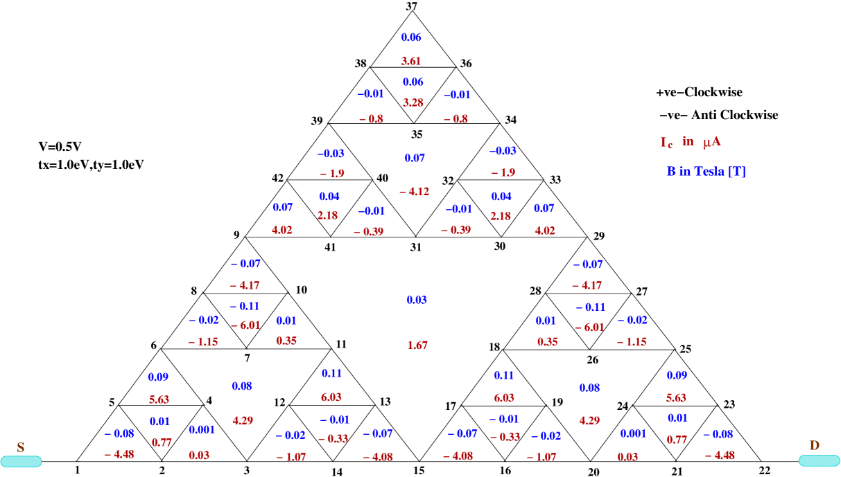
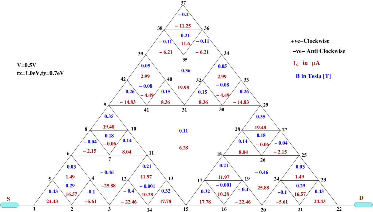
Figure 8: (Color online). Values of circular currents and associated magnetic fields at individual plaquettes of a $3$rd generation SPG ($N=42$) network. All the other physical parameters are mentioned in the figure.

Figure 5 exhibits the variation of circular current as well as magnetic field originating at the center due to this current in each plaquette for a smallest SPG fractal ($1$st generation) where $N=6$. The red and blue curves correspond to the isotropic and anisotropic cases respectively. Variation of circular current and magnetic field with bias voltage in individual loops can be seen clearly. Both these quantities behave in a similar manner, apart from a scale factor, and they cannot be predicted to be either increasing or decreasing consistently due to the introduction of anisotropy unlike the case of transport current. The spectra (a)-(d) indicate the situations where leads are connected at sites $1$ and $3$, while in (e)-(h) the results are shown when the leads are connected at the sites $1$ and $6$. Quite interestingly we find that the circular currents $I_{c1}$ (measured for the triangle connecting sites $1$, $2$ and $5$) and $I_{c2}$ (measured for the triangle connecting sites $2$, $3$ and $4$), and associated magnetic fields, $B_{1}$ and $B_{2}$, exhibit exactly identical variation with external bias voltage for both the isotropic and anisotropic cases yielding a mirror symmetry about an

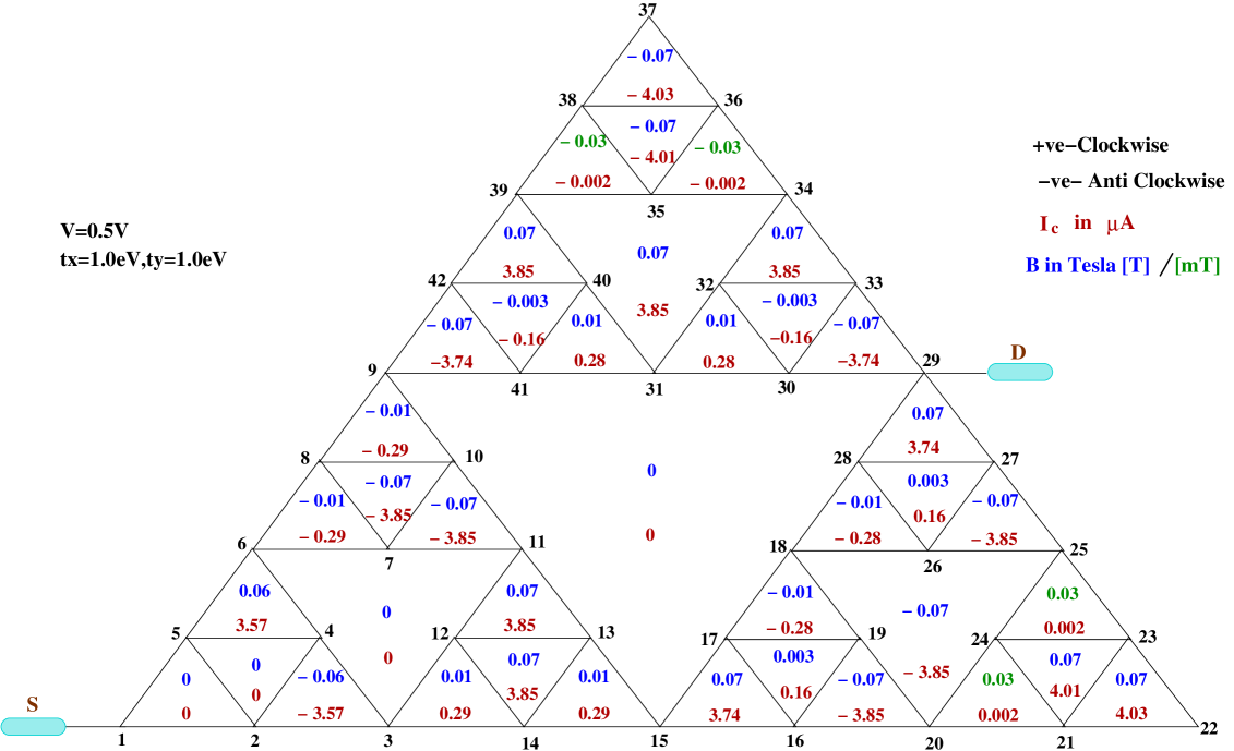
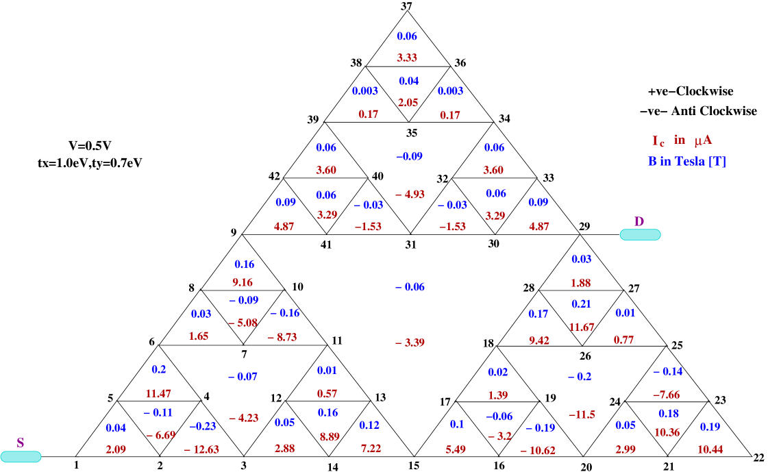
Figure 9: (Color online). Same as Fig. 8 with different source-SPG-drain configuration.

imaginary vertical axis dividing the SPG into two equal halves. This unique feature is observed only when leads are connected on either sides of the bases of SPG e.g., at positions $1$ and $3$ for this particular generation of the fractal. Analogous feature is also observed when leads are coupled to the sites ($1$, $15$) and ($1$, $22$) of $2$nd and $3$rd generations, respectively, and even valid for any higher generation. This mirror symmetry gets disturbed when the drain lead is connected elsewhere.

In the rest of our discussion we point out some interesting facts regarding the magnitudes of current and magnetic field for $2$nd and $3$rd generation

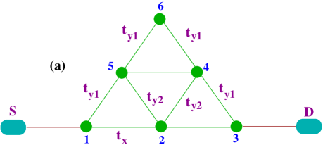
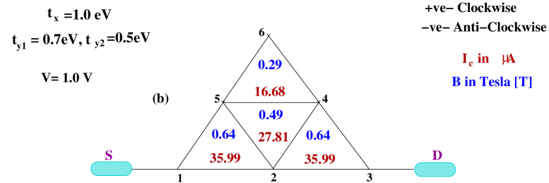
Figure 10: (Color online). Values of circular currents and associated magnetic fields in different triangular plaquettes for a $6$-site SPG network subjected to three different hopping integrals ($t_{x}$, $t_{y1}$ and $t_{y2}$). The schematic diagram of the network is shown in (a), while in (b) the numerical results are presented those are computed for a particular set of parameter values as given in this spectrum.

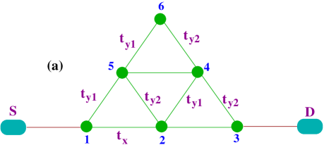
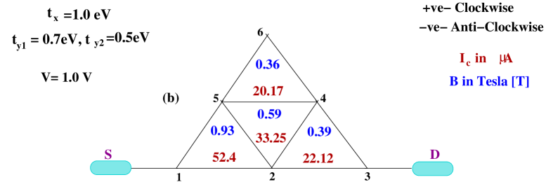
Figure 11: (Color online). Same as Fig. 10 with a different arrangement of two hopping integrals $t_{y1}$ and $t_{y2}$.

fractals. Figures 6-9 exhibit magnitudes of $I_{c}$ and $B$ at a typical bias voltage both in case of equal and unequal hoppings for these two generations. From Figs. 6 and 8 we see that mirror symmetry is preserved and it is obtained for any bias voltage which we confirm through our numerical calculations. Thus it is assured that this feature holds true for any generation. As soon as position of leads are changed the symmetry gets destroyed which is reflected from Figs. 7 and 9, and thus revealing a new feature that could not be detected in case of transport current. With increasing SPG generation both the loop current and magnetic field will decrease in magnitude.

Up to this we consider two types of hopping integrals (viz, $t_{x}$ and $t_{y}$) to discuss characteristic properties of circular current and associated magnetic field in different triangular plaquettes of SPG networks. From these results we establish when the mirror symmetry persists and under which situation it disappears. But, one question naturally comes how the mirror symmetry becomes affected if one considers the effect of two distinct hopping integrals (i.e., $t_{y1}$ and $t_{y2}$) along two different angular directions associated with two different angles, together with the horizontal hopping term $t_{x}$. To address this question in Figs. 10 and 11 we present the results of circular currents and associated magnetic fields in different triangular plaquettes for a $6$-site SPG network considering a particular set of parameter values. Two different arrangements of $t_{y1}$ and $t_{y2}$ are taken into account, those are schematically shown in Figs. 10(a) and Figs. 11(a), respectively, to have a complete idea about the mirror symmetry exhibited by $I_{c}$ and $B$. Very interestingly, we can see by comparing the results given in Figs. 10 and 11 that the mirror symmetry about an imaginary vertical line (passing through lattice sites $2$ and $6$) dividing the SPG into two equal halves exists only when the geometry itself is mirror symmetric about this imaginary line. This behavior is clearly reflected in any higher generation which we confirm through our extensive numerical calculations. Our analysis of circular and transport current gives a clear and interesting picture of the phenomena occurring in each individual triangles of the network.

From the presented results we see that the magnetic field originating at the center of each plaquette as a result of bias induced circular current exhibits several interesting patterns. For all the three generations studied here the magnitude of $B$ is much higher than $7\;$mT in almost all the loops except for few triangles, and it is very interesting since such an amount of magnetic field is sufficient to cause spin flipping Lidar . Therefore, if a spin is situated at the center of the plaquettes, induced magnetic field is sufficient enough to cause spin flipping and this information might be quiet useful in quantum computation and in spintronics applications. We hope by placing magnetic sites in individual plaquettes and considering the interaction of these local sites with the circular current induced magnetic fields efficient spin-polarized device can be designed in the near future.

IV Conclusion

We have investigated the phenomena of circulating currents in individual loops along with overall conductance of a Sierpinski gasket fractal in presence of external bias. The effect of self-similar structure on circular currents and associated magnetic fields have been studied considering different generations of the SPG network, and, we have found that for a particular source-SPG-drain configuration these quantities reveal definite regularity when the generation gets changed. Most importantly we have noted that the model provides mirror symmetry of current as well as magnetic field with respect to a plane perpendicular to the base line (as shown in Fig. 1), but this symmetry gets destroyed for other lead-SPG-lead configurations. Certainly it reveals a new feature which could not be detected by analyzing the junction current. In our discussion, we have considered both the isotropic and anisotropic cases, where the anisotropy has been introduced through the nearest-neighbor hopping integral. Quite interestingly we have noted that the inclusion of anisotropy in hopping integral causes an enhancement of overall junction current, which is quite different compared to the conventional systems where anisotropy or inhomogeneity causes a reduction of net current.

References

- (1) T. Ficker and P. Benesovský, Eur. J. Phys. 23, 403 (2002).
- (2) G. R. Newkome, P. Wang, C. N. Moorefield, T. J. Cho, P. P. Mohapatra, S. Li, S.-H. wang, O. Lukoy-anova, L. Echegoyen, J. A. Palagallo, V. Iancu, and S.-W. Hla, Science 312, 1782 (2006).
- (3) Y. Liu, Z. Hou, P. M. Hui, and W. Sritrakool, Phys. Rev. B 60, 13444 (1999).
- (4) Z. Lin, Y. Cao, Y. Liu, and P. M. Hui, Phys. Rev. B 66, 045311 (2002).
- (5) X. R. Wang, Phys. Rev. B 51, 9310 (1995).
- (6) S. K. Maiti and A. Chakrabarti, J. Comput. Theor. Nanosci. 10, 504 (2013).
- (7) P. Orellana and F. Claro, Phys. Rev. Lett. 90, 178302 (2003).
- (8) K. Tagami, L. Wang, and M. Tsukada, Nano Lett. 4, 209 (2004).
- (9) M. D. Ventra, N. D. Lang, and S. T. Pentelides, Chem. Phys. 281, 189 (2002).
- (10) M. D. Ventra, S. T. Pentelides, and N. D. Lang, Appl. Phys. Lett. 76, 3448 (2000).
- (11) A. Aviram and M. Ratner, Chem. Phys. Lett. 29, 277 (1974).
- (12) A. Nitzan and M. A. Ratner, Science 300, 1384 (2003).
- (13) S. Sil, S. K. Maiti, and A. Chakrabarti, Phys. Rev. Lett. 101, 076803 (2008)
- (14) S. Woitellier, J. P. Launay, and C. Joachim, Chem. Phys. 131, 481 (1989).
- (15) S. Nakanishi and M. Tsukada, Surf. Sci. 38, 305 (1999).
- (16) M. Tsukada, K. Tagami, K. Hirose, and N. Kobayashi, J. Phys. Soc. Jpn. 74, 1079 (2005).
- (17) A. M. Jayannavar and P. Singha Deo, Phys. Rev. B 51, 10175 (1995).
- (18) D. Rai, O. Hod, and A. Nitzan, J. Phys. Chem. C 114, 20583 (2010).
- (19) M. Büttiker, Y. Imry, and R. Landauer, Phys. Lett. A 96, 365 (1983).
- (20) H. F. Cheung, Y. Gefen, E. K. Reidel, and W. H. Shih, Phys. Rev. B 37, 6050 (1988).
- (21) P. A. Orellana, M. L. Ladrón de Guevara, M. Pacheco, and A. Latgé, Phys. Rev. B 68, 195321 (2003).
- (22) S. K. Maiti and A. Chakrabarti, Phys. Rev. B 82, 184201 (2010).
- (23) S. K. Maiti, Solid State Commun. 150, 2212 (2010).
- (24) V. Ambegaokar and U. Eckern, Phys. Rev. Lett. 65, 381 (1990).
- (25) A. Schmid, Phys. Rev. Lett. 66, 80 (1991).
- (26) U. Eckern and A. Schmid, Europhys. Lett. 18, 457 (1992).
- (27) I. Barth, J. Manz, Y. Shigeta, and K. Yagi, J. Am. Chem. Soc. 128, 7043 (2006).
- (28) I. Barth and J. Manz, Angew. Chem. Int. Ed. 45, 2962 (2006).
- (29) K. Nobusada and K. Yabana, Phys. Rev. A 75, 032518 (2007).
- (30) G. F. Quinteiro and J. Berakdar, Opt. Express 17, 20465 (2009).
- (31) A. Matos-Abiague and J. Berakdar, Phys. Rev. Lett. 94, 166801 (2005).
- (32) A. S. Moskalenko and J. Berakdar, Phys. Rev. B 80, 193407 (2009).
- (33) L. P. Levy, G. Dolan, J. Dunsmuir and H. Bouchiat, Phys. Rev. Lett. 64, 2074 (1990).
- (34) D. Mailly, C. Chapelier and A. Benoit, Phys. Rev. Lett. 70, 2020 (1993).
- (35) V. Chandrasekhar, R. A. Webb, M. J. Brady, M. B. Ketchen, W. J. Gallagher and A. Kleinsasser, Phys. Rev. Lett. 67, 3578 (1991).
- (36) S. Y. Cho, R. H. McKenzie, K. Kang, and C. K. Kim, J. Phys.: Condens. Matter 15, 1147 (2003).
- (37) D. A. Lidar and J. H. Thywissen, J. Appl. Phys. 96, 754 (2004).
- (38) Yu. V. Pershin and C. Piermarocchi, Phys. Rev. B 72, 245331 (2005).
- (39) E. V. Anda, G. Chiappe, and E. Louis, J. Appl. Phys. 111, 033711 (2012).
- (40) S. K. Maiti, J. Appl. Phys. 117, 024306 (2015).
- (41) S. Datta, Electronic transport in mesoscopic systems, Cambridge University Press, Cambridge (1997).
- (42) L. Wang, K. Tagami, and M. Tsukada, Jpn. J. Appl. Phys. 43, 2779 (2004).