Coulomb gluons and the ordering variable

Abstract

We study in detail the exchange of a Coulomb (Glauber) gluon in the first few orders of QCD perturbation theory in order to shed light on their accounting to all orders. We find an elegant cancellation of graphs that imposes a precise ordering on the transverse momentum of the exchanged Coulomb gluon.

1 Introduction

Large corrections to fixed-order matrix element calculations occur in perturbative QCD as a result of soft and/or collinear parton emissions. These can be calculated directly or using Monte Carlo event generators. The latter are multi-purpose and capture some, but not all, of the leading logarithmic behaviour via parton or dipole shower evolution. Interference between wide-angle soft gluon contributions can be included in the event generator approach but at the expense of ignoring contributions that are suppressed by powers of $1/N_{c}$. Most notably, Coulomb (a.k.a. Glauber) gluon exchanges are ignored.

In this paper we wish to study the physics of soft gluons beyond the leading colour approximation, and of particular interest will be the correct inclusion of Coulomb exchanges. It is well known that Coulomb exchanges are ultimately responsible for diffractive processes and the ambient particle production known as the “underlying event” Gaunt:2014ska . Moreover, attention has focussed on them due to the realization that they are the origin of the super-leading logarithms discovered in gaps-between-jets observables Forshaw:2006fk ; Forshaw:2008cq and later realized to affect almost all observables in hadron-hadron collisions Banfi:2010xy , as well as being the origin of a breakdown of collinear factorization catani2011 ; Forshaw:2012bi in hadron-hadron collisions.

Coulomb exchange should therefore be an important ingredient in any reasonably complete description of the partonic final state of hadron-hadron collisions. However, the inclusion of Coulomb exchanges in the standard shower algorithms is complicated because they mix colour and are non-probabilistic. Although there is a framework capable in principle of encompassing these corrections, Nagy:2007ty , the actual implementation of it Nagy:2012bt neglects them, as do other attempts to include sub-leading colour into parton showers Platzer:2012np .

It is not entirely clear how Coulomb exchanges should be included in an all-orders summation of soft gluon effects. The aim of this paper is to show how they can be included via a $k_{T}$-ordered evolution algorithm. We do not prove the correctness of the algorithm to all orders in perturbation theory but rather to the first two non-trivial orders. We think it is likely that the procedure generalizes to all orders.

The algorithm, for a general observable, is built from the set of cross sections corresponding to exclusive $n$ gluon emission, $\{\text{d}\sigma_{n}\}$:

$$\text{d}\sigma_{0} = \Bigl{\langle}M^{(0)}\Bigr{|}{\mathbf{V}}^{\dagger}_{0,Q}{\mathbf{V}}_{0,Q}\Bigl{|}M^{(0)}\Bigr{\rangle}~{}\text{d}\Pi_{0}$$

$$\text{d}\sigma_{1} = \Bigl{\langle}M^{(0)}\Bigr{|}{\mathbf{V}}^{\dagger}_{q_{1T},Q}\mathbf{D}_{1\mu}^{\dagger}{\mathbf{V}}^{\dagger}_{0,q_{1T}}{\mathbf{V}}_{0,q_{1T}}\mathbf{D}_{1}^{\mu}{\mathbf{V}}_{q_{1T},Q}\Bigl{|}M^{(0)}\Bigr{\rangle}~{}\text{d}\Pi_{0}\text{d}\Pi_{1}$$

$$\text{d}\sigma_{2} = \Bigl{\langle}M^{(0)}\Bigr{|}{\mathbf{V}}^{\dagger}_{q_{1T},Q}\mathbf{D}_{1\mu}^{\dagger}{\mathbf{V}}^{\dagger}_{q_{2T},q_{1T}}\mathbf{D}^{\dagger}_{2\nu}{\mathbf{V}}^{\dagger}_{0,q_{2T}}{\mathbf{V}}_{0,q_{2T}}\mathbf{D}_{2}^{\nu}{\mathbf{V}}_{q_{2T},q_{1T}}\mathbf{D}_{1}^{\mu}{\mathbf{V}}_{q_{1T},Q}\Bigl{|}M^{(0)}\Bigr{\rangle}~{}\text{d}\Pi_{0}\text{d}\Pi_{1}\text{d}\Pi_{2}$$ (1)

$$\mathrm{etc.}$$

To reveal the underlying simplicity of the structure we have used a very compact notation, which we now explain. The fixed-order matrix element is represented by a vector in colour and spin, denoted $\Bigl{|}M^{(0)}\Bigr{\rangle}$ and $\text{d}\Pi_{0}$ is the corresponding phase-space. Virtual gluon corrections are encoded in the Sudakov operator:

$${\mathbf{V}}_{a,b}=\exp\left[-\frac{2\alpha_{s}}{\pi}\int_{a}^{b}\frac{\text{d}k_{T}}{k_{T}}\sum_{i<j}(-\mathbb{T}_{i}\cdot\mathbb{T}_{j})\frac{1}{2}\left\{\int\frac{\text{d}y\,\text{d}\phi}{2\pi}\omega_{ij}-i\pi\;\Theta(ij=II~{}\mathrm{or}~{}FF)\right\}\right]~{},$$ (2)

where

$$\omega_{ij}=\frac{1}{2}k_{T}^{2}\frac{p_{i}\cdot p_{j}}{(p_{i}\cdot k)(p_{j}\cdot k)}$$ (3)

and the $\Theta$ term is unity for the case where partons $i$ and $j$ are either both in the initial state or both in the final state, and zero otherwise (this is the term corresponding to Coulomb exchange). The crucial ingredient of Eq. (2) is the fact that the limits on the transverse momenta of the virtual exchanges, $k_{T}$, are the transverse momenta of the emitted gluons. The colour charge of parton $i$ is denoted $\mathbb{T}_{i}$, and $k_{T}$, $y$ and $\phi$ are the transverse momentum, rapidity and azimuth of the virtual gluon with momentum $k$ that is exchanged between partons $i$ and $j$. The operator $\mathbf{D}_{i}^{\mu}$ corresponds to the real emission of a gluon with transverse momentum $q_{Ti}$ and the associated phase-space element (including a factor $\alpha_{s}$ for convenience) is $\text{d}\Pi_{i}$:

$$\mathbf{D}_{i}^{\mu} = \sum_{j}\mathbb{T}_{j}\;\frac{1}{2}q_{Ti}\frac{p_{j}^{\mu}}{p_{j}\cdot q_{i}}~{},$$

$$\text{d}\Pi_{i} = -\frac{2\alpha_{s}}{\pi}\frac{\text{d}q_{Ti}}{q_{Ti}}\frac{\text{d}y_{i}\text{d}\phi_{i}}{2\pi}~{}.$$ (4)

A general cross section can then be written

$$\sigma=\sum_{n=0}^{\infty}\int\text{d}\sigma_{n}\,F_{n}~{},$$ (5)

where $\{F_{n}\}$ are functions of the phase-space that define the observable. Although we have written formulae that are appropriate for soft gluon corrections, it is straightforward to extend them to include collinear emission too: the Sudakov operator ${\mathbf{V}}$ picks up a hard-collinear piece and the splitting operator $\mathbf{D}$ is modified.

Equation (1) is expressed as a chain of real emissions ordered in transverse momentum with Sudakov operators expressing the non-emission at intermediate scales. If we would ignore the Coulomb exchange contribution to the Sudakov operator then this would be the end of the story, in the sense that Eq. (1) encodes well-known physics. Moreover, if one takes the leading $N_{c}$ approximation then the colour evolution is diagonal and this drastically simplifies matters, allowing the computation of observables using a cross-section level shower algorithm, e.g. as is done in an event generator.

However, Coulomb exchanges are virtual corrections that do not correspond to a non-emission probability. In QED they exponentiate to an irrelevant phase in the scattering amplitude but this does not happen in the case of non-Abelian QCD. Since Coulomb gluons have transverse momentum but no rapidity or azimuth, it would seem most natural to include them as in Eq. (1). Indeed this is exactly what we assumed in Forshaw:2006fk ; Forshaw:2008cq ; Keates:2009dn , to compute the coefficient of the coherence violating super-leading logarithmic term in the “gaps between jets” observable. However, as pointed out in section 3.3 of Banfi:2010xy , it is possible to change the coefficient of the super-leading logarithm by limiting the $k_{T}$ integral of the Coulomb exchange by some other function of the real emission momenta. For example, the coefficient is divergent for energy ordering, zero for angular ordering and one-half of the $k_{T}$-ordered result in the case of virtuality ordering.

In the remainder of this paper, we will demonstrate that Eq. (1) is correct, at least to the first few orders in perturbation theory. To this end we will compute the amplitudes for one and two real gluon emissions to one-loop accuracy. Specifically, we perform Feynman-gauge calculations in order to check the correctness of the operators

$${\mathbf{V}}_{0,q_{1T}}\mathbf{D}_{1}^{\mu}{\mathbf{V}}_{q_{1T},Q}~{}~{}~{}\mathrm{and}~{}~{}~{}{\mathbf{V}}_{0,q_{2T}}\mathbf{D}_{2}^{\nu}{\mathbf{V}}_{q_{2T},q_{1T}}\mathbf{D}_{1}^{\mu}{\mathbf{V}}_{q_{1T},Q}~{}.$$ (6)

Since these expressions are to capture the leading soft behaviour, we work within the eikonal approximation for emissions off the fast partons involved in the hard sub-process. This is the only approximation we make and, in particular, we use the full triple-gluon vertex for soft gluon emissions off other soft gluons and we use the exact expressions for soft-gluon propagators. This means that we make no assumptions about the relative sizes of the momenta of real and virtual soft radiation.

For simplicity, we focus mainly on the case where $\Bigl{|}M^{(0)}\Bigr{\rangle}$ corresponds to two coloured incoming particles scattering into any number of colourless particles (e.g. the Drell-Yan process) and we only calculate the imaginary part of the loop integrals, since this corresponds to the contribution from Coulomb gluon exchange. Of course Coulomb exchange between the incoming hard partons is irrelevant at the cross-section level for scattering into a colourless final state, but our interest is at the amplitude level, where there remains much to learn. In particular, our calculations are sufficient to reveal the non-trivial way in which the real gluon transverse momenta serve to cut off the Coulomb gluon momentum. Moreover, since we will keep the full dependence on the colour matrices of the two incoming partons, our results give a clear indication of the structure of the more phenomenologically-interesting case of two coloured partons producing a system of coloured partons. We will perform the loop integrals over $k_{T}$ exactly and show that they result in precisely the two ($k_{T}$-ordered) terms in (6), up to non-logarithmic corrections. We will also see how the non-Abelian nature of QCD plays a crucial role in engineering the $k_{T}$ ordering.

Our focus in Section 2 is to make a check of the first term in (6), i.e. we consider the case of one real emission at one loop order. This section concludes by pointing out that $k_{T}$ ordering does not arise from the simplicity of the Drell-Yan process that we considered. Then we study the case of two real emissions, which provides a check of the second term in (6). Firstly, in Section 3, we describe the kinematic regions of interest and the behaviour of the tree-level amplitude. Then, in Section 4, we move to the one-loop case.

2 One real emission

The imaginary part of the one-loop, one-emission amplitude can be obtained from the cut graphs illustrated in Fig. 1. We subsequently refer to cuts that pass through the two fast parton lines as “eikonal cuts”. Note that there are no contributions arising from cuts through a fast parton and the Coulomb gluon, as we discuss briefly again towards the end of this section.

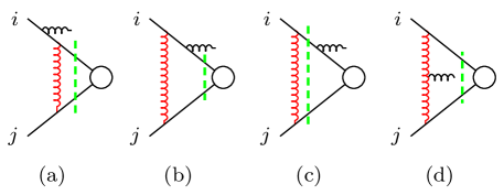
Figure 1: Four cut graphs contributing to the amplitude for real emission of a gluon, with four-momentum $q_{1}$ and colour $c_{1}$, off fast parton $i$. There are three further graphs corresponding to emission off fast parton $j$.

The contribution to the amplitude from graphs (a)–(c) is then

$$-\frac{i\pi}{8\pi^{2}}\frac{p_{i}\cdot\varepsilon_{1}}{p_{i}\cdot q_{1}}\Bigl{[}\mathbb{T}^{c_{1}}_{i}(\mathbb{T}_{i}\cdot\mathbb{T}_{j})-(\mathbb{T}_{i}\cdot\mathbb{T}_{j})\mathbb{T}_{i}^{c_{1}}+(\mathbb{T}_{i}\cdot\mathbb{T}_{j})\mathbb{T}_{i}^{c_{1}}\Bigr{]}\int_{0}^{Q^{2}}\frac{\text{d}k_{T}^{2}}{k_{T}^{2}}\;\Bigl{|}M^{(0)}\Bigr{\rangle}~{}.$$ (7)

Although the contribution from graphs (b) and (c) cancels, it is more instructive to keep them apart.

The notation is a little sloppy because we are not being clear about the space in which the colour charge operators act, but it should always be clear from the context. The integral of the Coulomb gluon momentum, $k_{T}$, is over the full range from 0 up to an ultraviolet scale that can be taken to be the hard scale, $Q$. Graph (d) is responsible for triggering the $k_{T}$ ordering. This is the only cut graph involving the triple-gluon vertex and it gives rise to the contribution:

$$-\frac{i\pi}{8\pi^{2}}\frac{p_{i}\cdot\varepsilon_{1}}{p_{i}\cdot q_{1}}\Bigl{[}(\mathbb{T}_{i}\cdot\mathbb{T}_{j})\mathbb{T}_{i}^{c_{1}}-\mathbb{T}_{i}^{c_{1}}(\mathbb{T}_{i}\cdot\mathbb{T}_{j})\Bigr{]}\int_{0}^{Q^{2}}\frac{\text{d}k_{T}^{2}}{k_{T}^{2}}\frac{q_{1T}^{2}}{k_{T}^{2}+q_{1T}^{2}}\;\Bigl{|}M^{(0)}\Bigr{\rangle}~{}.$$ (8)

Crucially, the loop integral of graph (d) acts as a switch. It is zero (i.e. sub-leading) if $k_{T}>q_{1T}$ and when it is active it has the effect of exactly cancelling the contribution from graphs (a) and (b). The result is that for $k_{T}>q_{1T}$ only graph (a) survives whilst for $k_{T}<q_{1T}$ only graph (c) survives, i.e. the final result is

$$-\frac{i\pi}{8\pi^{2}}\frac{p_{i}\cdot\varepsilon_{1}}{p_{i}\cdot q_{1}}\left[\mathbb{T}^{c_{1}}_{i}(\mathbb{T}_{i}\cdot\mathbb{T}_{j})\int_{q_{1T}^{2}}^{Q^{2}}\frac{\text{d}k_{T}^{2}}{k_{T}^{2}}+(\mathbb{T}_{i}\cdot\mathbb{T}_{j})\mathbb{T}_{i}^{c_{1}}\int_{0}^{q_{1T}^{2}}\frac{\text{d}k_{T}^{2}}{k_{T}^{2}}\right]\Bigl{|}M^{(0)}\Bigr{\rangle}~{}.$$ (9)

These contributions, with the Coulomb gluon $k_{T}$ restricted to be bounded by the $q_{1T}$ of the real emission are exactly in accordance with Eq. (1), i.e. after adding the contribution obtained after swapping $i\leftrightarrow j$ we get

$$\Bigl{[}\mathbb{J}_{1}(q_{1})\mathbb{C}_{q_{1T},Q}+\mathbb{C}_{0,q_{1T}}\mathbb{J}_{1}(q_{1})\Bigr{]}\Bigl{|}M^{(0)}\Bigr{\rangle}~{},$$ (10)

where $\mathbb{J}_{1}(q_{1})$ is the real emission operator:

$$\mathbb{J}_{1}^{c_{1}}(q_{1})\equiv\mathbb{T}^{c_{1}}_{i}\frac{p_{i}\cdot\varepsilon_{1}}{p_{i}\cdot q_{1}}+\mathbb{T}^{c_{1}}_{j}\frac{p_{j}\cdot\varepsilon_{1}}{p_{j}\cdot q_{1}},$$ (11)

and the Coulomb exchange operator $\mathbb{C}_{a,b}$ is

$$\mathbb{C}_{a,b}\equiv-\frac{i\pi\,\mathbb{T}_{i}\cdot\mathbb{T}_{j}}{8\pi^{2}}\int_{a^{2}}^{b^{2}}\frac{\text{d}k_{T}^{2}}{k_{T}^{2}}~{}.$$ (12)

Of particular note is the way that the unwanted cut of graph (b) always cancels, either against graph (c) or graph (d). Such a contribution would be problematic for any local evolution algorithm, since it corresponds to a Coulomb exchange retrospectively putting on-shell a pair of hard partons earlier in the evolution chain.

There is another way to think about this physics. The Coulomb exchange corresponds to on-shell scattering of the incoming partons long before the hard scattering and the real emission can occur either as part of this initial-state scattering or, much later, as part of the hard scattering. These two possibilities are illustrated in Fig. 2.

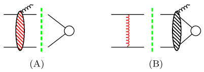
Figure 2: The two cuts corresponding to the two different physical mechanisms for single gluon emission.

Graphs (a), (b) and (d) of Fig. 1 are of type (A) and, in the domain where (d) is active, it cancels the other graphs. This means that the $k_{T}$ of the Coulomb gluon must be greater than that of the real emission, i.e. it is as if the real emission is occurring coherently off a hard partonic subprocess mediated by the Coulomb gluon. The sum over cuts of type (A) gives

$$-\frac{i\pi}{8\pi^{2}}\mathbb{T}_{j}^{b}(if_{c_{1}ba})\mathbb{T}_{i}^{a}\left[\frac{p_{i}\cdot\varepsilon_{1}}{p_{i}\cdot q_{1}}-\frac{p_{j}\cdot\varepsilon_{1}}{p_{j}\cdot q_{1}}\right]\int_{q_{1T}^{2}}^{Q^{2}}\frac{\text{d}k_{T}^{2}}{k_{T}^{2}}\Bigl{|}M^{(0)}\Bigr{\rangle}~{}.$$ (13)

Graph (c) is the only graph of type (B). In this case the real emission occurs much later than the Coulomb exchange, which therefore knows nothing of the emission and so its $k_{T}$ can take any value, i.e.

$$\mathbb{C}_{0,Q}\;\mathbb{J}_{1}(q_{1})\Bigl{|}M^{(0)}\Bigr{\rangle}~{}.$$ (14)

These contributions are separately gauge invariant, as can be seen by making the replacement $\varepsilon_{1}\to q_{1}$ in (13) and noting also that $(\mathbb{T}_{i}+\mathbb{T}_{j})\Bigl{|}M^{(0)}\Bigr{\rangle}=0$ in (14), which is a statement of colour conservation.

There is a third type of cut that appears at intermediate steps of the evaluation of some Feynman diagrams, in which the cut passes through a fast parton and a soft gluon. This corresponds to an unphysical (“wrongly time ordered”) process in which a gluon is emitted during the hard process and this gluon scatters off one of the incoming partons long before it was emitted. All such contributions to each diagram cancel and we can neglect them, leaving only the cuts of types (A) and (B).

To conclude this section, we comment on a trivial but important generalization of expression (10) to the case of coloured particles in the final state. Specifically, it follows that

$$\Bigl{[}\widetilde{\mathbb{J}}_{1}(q_{1})\mathbb{C}_{q_{1T},Q}+\mathbb{C}_{0,q_{1T}}\widetilde{\mathbb{J}}_{1}(q_{1})\Bigr{]}\Bigl{|}\widetilde{M}^{(0)}\Bigr{\rangle}$$ (15)

is the imaginary part of the amplitude for one soft gluon emission off a general hard sub-process with a Coulomb exchange in the initial state. Here, $\Bigl{|}\widetilde{M}^{(0)}\Bigr{\rangle}$ corresponds to two incoming hard partons scattering into any number of hard coloured partons and $\widetilde{\mathbb{J}}_{1}(q_{1})$ is the total real emission operator, i.e. including the cases where the gluon is emitted off a final-state hard parton. This result follows directly after noting that the emission operator from final-state partons commutes with the Coulomb exchange in the initial state and that $\mathbb{C}_{0,Q}=\mathbb{C}_{0,q_{1T}}+\mathbb{C}_{q_{1T},Q}$.

3 Two emissions at tree level

We now turn to the case of two real emissions, for which the transverse momentum ordering property is no longer an exact result. Instead, it is a property of the amplitude in certain regions of the phase-space of the emitted gluons. We will discuss these regions in the next subsection, after which we will proceed to study the behaviour of the amplitude at tree level. This will provide the foundation for the calculation, which appears in the next section, of the two-gluon emission amplitude with a Coulomb exchange.

3.1 Phase-space limits

Throughout this paper we will focus upon the following three limits. All of them correspond to a strong ordering in the transverse momenta of the real emissions, i.e. $q_{1T}\gg q_{2T}$. In terms of light-cone variables, the three limits are:

• Limit 1: Both emissions are at wide angle but one gluon is much softer than the other, i.e. $(q_{1}^{\pm}\sim q_{1T})\gg(q_{2}^{\pm}\sim q_{2T})$. Specifically, we take $q_{2}\to\lambda q_{2}$ and keep the leading term for small $\lambda$.

• Limit 2: One emission ($q_{2}$) collinear with $p_{i}$ by virtue of its small transverse momentum and the other ($q_{1}$) at a wide angle, i.e. $q_{2}^{+}\gg q_{2T}$ and $q_{1}^{+}\sim q_{1T}\gg q_{2T}$. Specifically, we take $q_{2}\to(q_{2}^{+},\lambda^{2}q_{2T}^{2}/(2q_{2}^{+}),\lambda\mathbb{q}_{2T})$ and keep the leading term for small $\lambda$.

• Limit 3: One emission ($q_{1}$) collinear with $p_{i}$ by virtue of its high energy and the other ($q_{2}$) at a wide angle, i.e. $q_{1}^{+}\gg q_{1T}$ and $q_{1T}\gg q_{2T}\sim q_{2}^{+}$. Specifically, we take $q_{1}\to(q_{1}^{+}/\lambda,\lambda q_{1T}^{2}/(2q_{1}^{+}),\mathbb{q}_{1T})$ and $q_{2}\to\lambda q_{2}$, and keep the leading term for small $\lambda$.

When we consider the leading behaviour of the amplitude, either at tree or one-loop level, we will make an expansion for small $\lambda$, keeping only the leading terms. With the exception of Section 4.4, we work with the following choice of polarisation vectors for the emitted gluons:

$$\varepsilon_{\mu}(q,\perp) = \frac{\epsilon_{\mu\nu\alpha\beta}q^{\nu}p_{i}^{\alpha}p_{j}^{\beta}}{\sqrt{2p_{i}\cdot p_{j}\,p_{i}\cdot q\,p_{j}\cdot q}}~{},$$

$$\varepsilon^{\mu}(q,\parallel) = \frac{q\cdot p_{j}\,p_{i}^{\mu}-q\cdot p_{i}\,p_{j}^{\mu}-p_{i}\cdot p_{j}\,q^{\mu}}{\sqrt{2p_{i}\cdot p_{j}\,p_{i}\cdot q\,p_{j}\cdot q}}~{}.$$ (16)

In limits 2 and 3, only $\varepsilon^{\mu}(q,\parallel)$ of the collinear parton, gives rise to a leading contribution.

Limit 3 is of particular interest because it is the limit that gives rise to the super-leading logarithms Forshaw:2006fk ; Forshaw:2008cq . It is worth noting that although $q_{1T}\gg q_{2T}$ in all three limits, we may have $q_{1}^{+}\sim q_{2}^{+}$ in limit 2 and $q_{1}^{-}\sim q_{2}^{-}$ in limit 3. This means that limits 2 and 3 are not sub-limits of limit 1 in any trivial way. We will see that different Feynman diagrams contribute differently in the different limits. It is therefore remarkable that the final result is identical in all three limits. Although we have not yet proven it, we suspect that the final results may well hold in the more general case in which only $q_{1T}\gg q_{2T}$.

3.2 Tree-level amplitude

The tree-level amplitude with two soft gluon emissions $\Bigl{|}M^{(0)}_{2}\Bigr{\rangle}$ can be expressed Catani:1999ss in terms of an operator $\mathbb{K}_{2}(q_{1},q_{2})$ that acts on the hard process to insert two real emissions, i.e.

$$\Bigl{|}M^{(0)}_{2}\Bigr{\rangle}=\mathbb{K}_{2}(q_{1},q_{2})\Bigl{|}M^{(0)}\Bigr{\rangle}~{}.$$ (17)

In the case of only two incoming hard partons, we must consider the four graphs shown in Fig. 3 plus four further graphs corresponding to the interchange $i\leftrightarrow j$. As we will now show, $\mathbb{K}_{2}$ simplifies in each of the limits 1–3 to a product of two single emission operators.

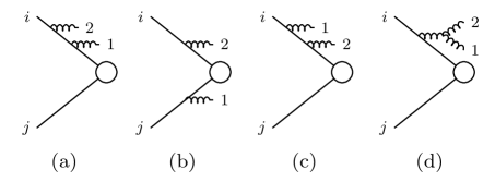
Figure 3: The case of two real emissions. There are four more graphs obtained by swapping $(i\leftrightarrow j)$.

Let us consider first the leading behaviour in limit 1. In this region only graphs (a), (b) and (d) in Fig. 3 are leading. They give

$$\mathbb{K}^{c_{1},c_{2}}_{2}(q_{1},q_{2})=\left[\frac{\mathbb{T}_{i}^{c_{2}}p_{i}\cdot\varepsilon_{2}}{p_{i}\cdot q_{2}}\frac{\mathbb{T}_{i}^{c_{1}}p_{i}\cdot\varepsilon_{1}}{p_{i}\cdot q_{1}}\right]+\left[\frac{\mathbb{T}_{i}^{c_{2}}p_{i}\cdot\varepsilon_{2}}{p_{i}\cdot q_{2}}\frac{\mathbb{T}_{j}^{c_{1}}p_{j}\cdot\varepsilon_{1}}{p_{j}\cdot q_{1}}\right]$$ (18)

$$\hskip 50.00008pt+\left[\frac{if^{c_{1}c_{2}a}q_{1}\cdot\varepsilon_{2}}{q_{1}\cdot q_{2}}\frac{\mathbb{T}_{i}^{a}p_{i}\cdot\varepsilon_{1}}{p_{i}\cdot q_{1}}-\frac{if^{c_{1}c_{2}a}\mathbb{T}_{i}^{a}\varepsilon_{1}\cdot\varepsilon_{2}}{2q_{1}\cdot q_{2}}\right]+(i\leftrightarrow j)~{}.$$

The $\varepsilon_{1}\cdot\varepsilon_{2}$ term vanishes when it acts upon $\Bigl{|}M^{(0)}\Bigr{\rangle}$ due to colour conservation. The leading behaviour can thus be written

$$\Bigl{|}M^{(0)}_{2}\Bigr{\rangle} = \mathbb{J}_{2}^{c_{2}c_{1}a}(q_{2},q_{1})\mathbb{J}_{1}^{a}(q_{1})\Bigl{|}M^{(0)}\Bigr{\rangle}~{},$$ (19a)

$$\mathbb{J}_{2}^{c_{2}c_{1}a}(q_{2},q_{1}) \equiv \mathbb{J}_{1}^{c_{2}}(q_{2})\delta^{c_{1}a}+\frac{if^{c_{1}c_{2}a}\;q_{1}\cdot\varepsilon_{2}}{q_{1}\cdot q_{2}},$$ (19b)

where $\mathbb{J}_{2}^{c_{2}c_{1}a}(q_{2},q_{1})$ is the operator that adds a second soft gluon $(q_{2})$.

In limit 2 only the first two graphs in Fig. 3 are leading and they can be written

$$\Bigl{|}M^{(0)}_{2}\Bigr{\rangle}=\left[\frac{\mathbb{T}_{i}^{c_{2}}p_{i}\cdot\varepsilon_{2}}{p_{i}\cdot q_{2}}\right]\mathbb{J}_{1}^{c_{1}}(q_{1})\Bigl{|}M^{(0)}\Bigr{\rangle}~{}.$$ (20)

This is exactly what is obtained by taking the collinear limit $q_{2}\parallel p_{i}$ in the expression for limit 1, Eq. (19a).

We now turn our attention to limit 3. The leading contributions are graphs (a), (c) and (d), and the $(i\leftrightarrow j)$ permutation of graph (b) in Fig. 3. These four contributions (in order) sum to

$$\mathbb{K}_{2}^{c_{1},c_{2}}(q_{1},q_{2})=\left[\frac{\mathbb{T}_{i}^{c_{2}}\varepsilon_{2}^{-}}{q_{2}^{-}}\frac{\mathbb{T}_{i}^{c_{1}}\varepsilon_{1}^{-}}{q_{1}^{-}+q_{2}^{-}}\right]+\left[\frac{\mathbb{T}_{i}^{c_{1}}\varepsilon_{1}^{-}}{q_{1}^{-}}\frac{\mathbb{T}_{i}^{c_{2}}\varepsilon_{2}^{-}}{q_{1}^{-}+q_{2}^{-}}\right]$$

$$\hskip 50.00008pt+\left[\frac{if^{c_{1}c_{2}a}\;\varepsilon_{2}^{-}}{q_{2}^{-}}\frac{\mathbb{T}_{i}^{a}\varepsilon_{1}^{-}}{q_{1}^{-}+q_{2}^{-}}\right]+\left[\frac{\mathbb{T}_{j}^{c_{2}}\varepsilon_{2}^{+}}{q_{2}^{+}}\frac{\mathbb{T}_{i}^{c_{1}}\varepsilon_{1}^{-}}{q_{1}^{-}}\right]~{}.$$ (21)

At first glance it seems like an interpretation in terms of a product of single emission operators is not possible any more. However, using $\mathbb{T}_{i}^{c_{1}}\mathbb{T}_{i}^{c_{2}}=\mathbb{T}_{i}^{c_{2}}\mathbb{T}_{i}^{c_{1}}+if^{c_{1}c_{2}a}\mathbb{T}_{i}^{a}$, the contribution of graph (c) can be written

$$\frac{\mathbb{T}_{i}^{c_{1}}\varepsilon_{1}^{-}}{q_{1}^{-}}\frac{\mathbb{T}_{i}^{c_{2}}\varepsilon_{2}^{-}}{q_{1}^{-}+q_{2}^{-}}=\left[\frac{\mathbb{T}_{i}^{c_{2}}\varepsilon_{2}^{-}}{q_{1}^{-}}\frac{\mathbb{T}_{i}^{c_{1}}\varepsilon_{1}^{-}}{q_{1}^{-}+q_{2}^{-}}\right]+\left[\frac{if^{c_{1}c_{2}a}\varepsilon_{2}^{-}}{q_{1}^{-}}\frac{\mathbb{T}_{i}^{a}\varepsilon_{1}^{-}}{q_{1}^{-}+q_{2}^{-}}\right]~{}.$$ (22)

The light cone variables make clear the fact that the two terms on the right-hand side have the same dependence on colour and spin as the first term on each line of Eq. (21). Their momentum dependence can be combined using

$$\frac{1}{q_{1}^{-}}\frac{1}{q_{1}^{-}+q_{2}^{-}}+\frac{1}{q_{2}^{-}}\frac{1}{q_{1}^{-}+q_{2}^{-}}=\frac{1}{q_{1}^{-}}\frac{1}{q_{2}^{-}}~{},$$ (23)

to give

$$\Bigl{|}M^{(0)}_{2}\Bigr{\rangle}=\mathbb{J}_{2\;}^{c_{1}c_{2}a}(q_{2},q_{1})\left(\frac{\mathbb{T}_{i}^{a}p_{i}\cdot\varepsilon_{1}}{p_{i}\cdot q_{1}}\right)\Bigl{|}M^{(0)}\Bigr{\rangle}~{}.$$ (24)

As in the case of limit 2, this can be obtained by taking the collinear limit $q_{1}\parallel p_{i}$ in Eq. (19a). Remarkably, we will have the same property at one-loop order, i.e. the leading expressions in limits 2 and 3 can be reached by taking the relevant collinear limit of the leading expression in limit 1. This is particularly non-trivial in limit 3, because the leading graphs are not a subset of those in limit 1.

Figure 4 shows how the graphs in Fig. 3 can be projected onto three spin and colour structures. These particular structures are special because the net projection onto each can be represented in terms of a product of two single emission operators.

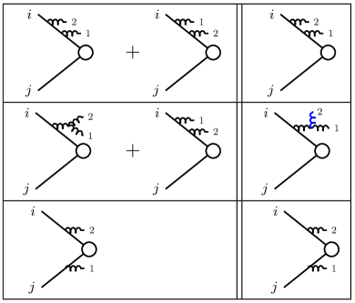
Figure 4: Diagrammatic representation of how to group the graphs in order to write the final result as a product of single emission operators. There are three further structures, obtained by exchanging $i\leftrightarrow j$.

Each grouping of graphs is associated with a specific spin and colour structure, which can be read off from the graph at the end of each row. These are

$$\left\{\frac{\mathbb{T}_{i}^{c_{2}}p_{i}\cdot\varepsilon_{2}}{p_{i}\cdot q_{2}}\frac{\mathbb{T}_{i}^{c_{1}}p_{i}\cdot\varepsilon_{1}}{p_{i}\cdot q_{1}},\frac{if^{c_{1}c_{2}a}\;q_{1}\cdot\varepsilon_{2}}{q_{1}\cdot q_{2}}\frac{\mathbb{T}_{i}^{a}p_{i}\cdot\varepsilon_{1}}{p_{i}\cdot q_{1}},\frac{\mathbb{T}_{i}^{c_{2}}p_{i}\cdot\varepsilon_{2}}{p_{i}\cdot q_{2}}\frac{\mathbb{T}_{j}^{c_{1}}p_{j}\cdot\varepsilon_{1}}{p_{j}\cdot q_{1}}\right\}+\{(i\leftrightarrow j)\}~{}.$$ (25)

In limit 3, the two diagrams on each of the first two lines of Fig. 4 combine to give each effective diagram on the right, interpreted as if the two emissions were independent. Equivalently, they conspire to act as if $q_{1}^{-}$ and $q_{2}^{-}$ were strongly ordered, even though they are not. It is this fact that allows the limit 3 result to be obtained from the limit 1 result (in which they are strongly ordered).

4 Two emissions at one loop

We now consider the one-loop amplitude for a hard process with two incoming partons and two soft emissions. In contrast to the single real emission case, we must now consider graphs with cuts through two soft gluon lines, i.e. corresponding to a Coulomb exchange between the two outgoing soft gluons.

4.1 Eikonal cuts

Figure 5 illustrates the three gauge-invariant classes of cut graph, where the cut is through the two hard partons. As before, we refer to these as eikonal cuts. The corresponding amplitudes can be reduced to transverse momentum integrals. In order to regulate the diagrams that do not involve any emissions off the virtual gluon, we introduce an ultraviolet cutoff of $Q^{2}$. In all cases we regularize the infrared divergences by analytically continuing the dimension of the transverse momentum integral $\text{d}^{2}k_{T}\to\text{d}^{d-2}k_{T}$.

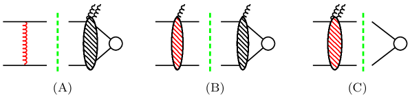
Figure 5: The three cuts corresponding to the three different physical mechanisms for double-gluon emission. Each of these cuts is gauge invariant.

We start by simply stating the bottom line. The remainder of this section will be devoted to examining how these results arise. The complete calculation involves explicitly computing the diagrams Fig. 7 in dimensional regularization (using Ellis:2011cr ; Huber:2007dx ) and without any approximation except the eikonal approximation.

The leading behaviour arising from eikonal cuts in limit 1 is

$$\bigg{[}\mathbb{C}_{0,q_{2T}}\mathbb{J}_{2}^{c_{2}c_{1}a}(q_{2},q_{1})\mathbb{J}_{1}^{a}(q_{1})+\mathbb{J}_{2}^{c_{2}c_{1}a}(q_{2},q_{1})\mathbb{C}_{q_{2T},q_{1T}}\mathbb{J}_{1}^{a}(q_{1})$$

$$+\mathbb{J}_{2}^{c_{2}c_{1}a}(q_{2},q_{1})\mathbb{J}_{1}^{a}(q_{1})\mathbb{C}_{q_{1T},Q}\bigg{]}\Bigl{|}M^{(0)}\Bigr{\rangle}~{},$$ (26)

where the current $\mathbb{J}_{2}^{c_{2}c_{1}a}(q_{2},q_{1})$ is defined in Eq. (19b). This expression is the expected generalization of the one-emission case (10) and the key point is that the $k_{T}$ of the Coulomb exchange is ordered with respect to the real-emission transverse momenta. For the first two terms, the vector $\mathbb{J}_{1}^{a}(q_{1})\Bigl{|}M^{(0)}\Bigr{\rangle}$ acts as a hard subprocess for the second gluon emission, i.e. as in Eq. (15) with $q_{1T}$ playing the role of $Q$.

Similarly, in limit 2 the sum over eikonal cuts gives

$$\bigg{[}\mathbb{C}_{0,q_{2T}}\left[\frac{\mathbb{T}_{i}^{c_{2}}\;p_{i}\cdot\varepsilon_{2}}{p_{i}\cdot q_{2}}\right]\mathbb{J}_{1}^{c_{1}}(q_{1})+\left[\frac{\mathbb{T}_{i}^{c_{2}}\;p_{i}\cdot\varepsilon_{2}}{p_{i}\cdot q_{2}}\right]\mathbb{C}_{q_{2T},q_{1T}}\mathbb{J}_{1}^{c_{1}}(q_{1})$$

$$+\left[\frac{\mathbb{T}_{i}^{c_{2}}\;p_{i}\cdot\varepsilon_{2}}{p_{i}\cdot q_{2}}\right]\mathbb{J}_{1}^{c_{1}}(q_{1})\mathbb{C}_{q_{1T},Q}\bigg{]}\Bigl{|}M^{(0)}\Bigr{\rangle}~{},$$ (27)

whilst in limit $3$ the result is

$$\bigg{[}\mathbb{C}_{0,q_{2T}}\mathbb{J}_{2}^{c_{2}c_{1}a}(q_{2},q_{1})\left[\frac{\mathbb{T}_{i}^{a}\;p_{i}\cdot\varepsilon_{1}}{p_{i}\cdot q_{1}}\right]+\mathbb{J}_{2}^{c_{2}c_{1}a}(q_{2},q_{1})\mathbb{C}_{q_{2T},q_{1T}}\left[\frac{\mathbb{T}_{i}^{a}\;p_{i}\cdot\varepsilon_{1}}{p_{i}\cdot q_{1}}\right]$$

$$+\mathbb{J}_{2}^{c_{2}c_{1}a}(q_{2},q_{1})\left[\frac{\mathbb{T}_{i}^{a}\;p_{i}\cdot\varepsilon_{1}}{p_{i}\cdot q_{1}}\right]\mathbb{C}_{q_{1T},Q}\bigg{]}\Bigl{|}M^{(0)}\Bigr{\rangle}~{}.$$ (28)

As in the tree-level case, the leading behaviour in limits 2 and 3 coincides with the expressions that result from taking the relevant collinear limit of the leading expression in limit 1. These results confirm the conjecture that Eq. (1) correctly reproduces the sum over eikonal cuts, although, as we will shortly see, the way that the $k_{T}$ ordering establishes itself is rather involved.

In order to see our way to Eq. (1) we must understand how to deal with the graphs involving the triple-gluon vertex. In the simpler case of only one real emission, this is illustrated in Fig. 6, which illustrates how the Feynman gauge graphs are to be grouped together and projected onto the relevant spin and colour tensors.

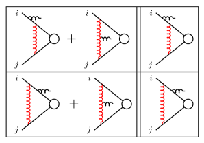
Figure 6: Diagrammatic representation of how to group the graphs that give rise to the transverse momentum ordered expression (10). Two more structures are obtained by permuting $(i\leftrightarrow j)$.

The corresponding amplitudes are

$$\left\{\frac{\mathbb{T}_{i}\;p_{i}\cdot\varepsilon}{p_{i}\cdot q_{1}}\;\frac{-i\pi\;\mathbb{T}_{j}\cdot\mathbb{T}_{i}}{8\pi^{2}},\frac{-i\pi\;\mathbb{T}_{j}\cdot\mathbb{T}_{i}}{8\pi^{2}}\;\;\frac{\mathbb{T}_{i}\;p_{i}\cdot\varepsilon}{p_{i}\cdot q_{1}}\right\}+\left\{(i\leftrightarrow j)\right\}.$$ (29)

The single graph involving the triple gluon vertex is thus shared out between all four contributing tensors.

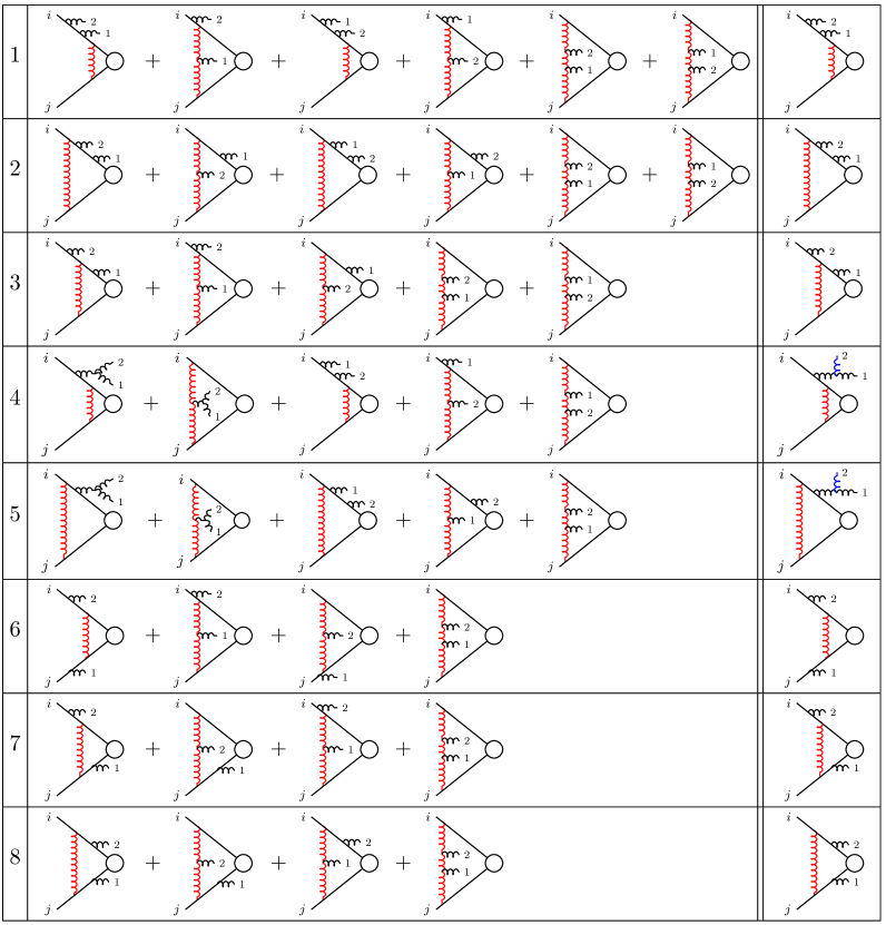
Figure 7: Diagrammatic representation of how to group the graphs that give rise to the transverse momentum-ordered expression in the case of two emissions at one loop. There are 12 more structures to consider: 8 are obtained by permuting $(i\leftrightarrow j)$ and the other four are obtained by permuting $(1\leftrightarrow 2)$ and $(i\leftrightarrow j,1\leftrightarrow 2)$ in groups 3 and 7.

Figure 7 is the generalization of Fig. 4 and Fig. 6. By way of illustration, the tensor corresponding to the first graph in the first row of the figure is

$$\;\frac{\mathbb{T}_{i}^{c_{2}}\;p_{i}\cdot\varepsilon_{2}}{p_{i}\cdot q_{2}}\;\frac{\mathbb{T}_{i}^{c_{1}}\;p_{i}\cdot\varepsilon_{1}}{p_{i}\cdot q_{1}}\;\frac{-i\pi\;\mathbb{T}_{i}\cdot\mathbb{T}_{j}}{8\pi^{2}}.$$ (30)

In limits 1–3, every row in Fig. 7 either adds up to a subleading expression or to one of the terms in Eqs. (26)–(28). This figure contains all of the leading contributions arising from the 36 different graphs with eikonal cuts.

In order to illustrate how the transverse momentum ordered integrals arise, we will consider two examples in some detail. We start by taking a closer look at the first row of six graphs in Fig. 7. All of these graphs have only a single cut, corresponding to production mechanism (C) in Fig. 5. The first graph of the six gives rise to a factor of

$$G_{11}=\frac{q_{1}^{-}}{(q_{2}^{-}+q_{1}^{-})}\int_{0}^{Q^{2}}\frac{\text{d}k_{T}^{2}}{k_{T}^{2}}~{}.$$ (31)

The factor multiplying the integral simplifies to unity in the case of limits 1 and 2 but not in limit 3, where $q_{1}^{-}$ and $q_{2}^{-}$ could be of the same order. The projection of the third graph gives

$$G_{13}=\frac{q_{2}^{-}}{(q_{1}^{-}+q_{2}^{-})}\int_{0}^{Q^{2}}\frac{\text{d}k_{T}^{2}}{k_{T}^{2}}$$ (32)

and this is only leading in the case of limit 3. Obviously these Abelian-like contributions place no restriction on the $k_{T}$ of the Coulomb exchange. Note that

$$G_{11}+G_{13}=\int_{0}^{Q^{2}}\frac{\text{d}k_{T}^{2}}{k_{T}^{2}}.$$ (33)

The second graph is the first involving the triple gluon vertex. It gives

$$G_{12}=-\left[\int_{0}^{2q_{1}^{-}q_{2}^{+}}\frac{\text{d}k_{T}^{2}}{k_{T}^{2}}+\frac{q_{2}^{-}-q_{1}^{-}}{q_{2}^{-}+q_{1}^{-}}\int_{0}^{2(q_{1}^{+}+q_{2}^{-})^{2}q_{2}^{+}/q_{1}^{-}}\frac{\text{d}k_{T}^{2}}{k_{T}^{2}}\right]~{}.$$ (34)

We note that the Coulomb integral cannot be written purely in terms of transverse momenta. However, the fourth graph is obtained from the second by interchanging $q_{1}$ and $q_{2}$. Thus the sum of graphs 2 and 4 is

$$G_{12}+G_{14}=-\frac{1}{(q_{1}^{-}+q_{2}^{-})}\left[q_{2}^{-}\int_{0}^{q_{2T}^{2}}\frac{\text{d}k_{T}^{2}}{k_{T}^{2}}+q_{1}^{-}\int_{0}^{q_{1T}^{2}}\frac{\text{d}k_{T}^{2}}{k_{T}^{2}}\right]~{}.$$ (35)

Graphs 5 and 6 also combine to produce a reasonably compact result involving the azimuthal angle between $q_{1T}$ and $q_{2T}$. It is sub-leading in limits 1 and 2, and in limit 3 it simplifies to

$$G_{15}+G_{16}\approx-\frac{q_{2}^{-}}{(q_{1}^{-}+q_{2}^{-})}\int_{q_{2T}^{2}}^{q_{1T}^{2}}\frac{\text{d}k_{T}^{2}}{k_{T}^{2}}~{}.$$ (36)

Now we can combine the graphs. In limits 1 and 2 only $G_{11}$ and $G_{14}$ contribute, with the latter contributing only for $k_{T}<q_{1T}$, exactly as in the one emission case. The two combine to give

$$\int_{q_{1T}^{2}}^{Q^{2}}\frac{\text{d}k_{T}^{2}}{k_{T}^{2}}~{},$$ (37)

which is exactly as expected. Limit 3 is more subtle and involves the interplay of all 6 graphs. Remarkably, the sum of these is also exactly equal to (37). The key is the way graphs 5 and 6 serve to extend the upper limit in the first of the two terms in Eq. (35) from $q_{2T}^{2}$ to $q_{1T}^{2}$, so that the net effect of all four graphs involving the triple-gluon vertex is merely to cut out the region with $k_{T}<q_{1T}$.

It is also instructive to look at the graphs in the third row of Fig. 7. These involve cuts of type (B) and (C) in Fig. 5. We will just state the results (the subscripts $B$ and $C$ refer to the cut):

$$G_{31B}=\int_{0}^{Q^{2}}\frac{\text{d}k_{T}^{2}}{k_{T}^{2}}=-G_{31C}~{},$$ (38)

$$G_{32}+G_{33C}=\frac{1}{(q_{1}^{-}+q_{2}^{-})}\left[q_{2}^{-}\int_{0}^{q_{2T}^{2}}\frac{\text{d}k_{T}^{2}}{k_{T}^{2}}+q_{1}^{-}\int_{0}^{q_{1T}^{2}}\frac{\text{d}k_{T}^{2}}{k_{T}^{2}}\right],$$ (39)

$$G_{33B}=-\int_{0}^{q_{2T}^{2}}\frac{\text{d}k_{T}^{2}}{k_{T}^{2}}~{},$$ (40)

so that

$$G_{32}+G_{33}=\frac{q_{1}^{-}}{(q_{1}^{-}+q_{2}^{-})}\int_{q_{2T}^{2}}^{q_{1T}^{2}}\frac{\text{d}k_{T}^{2}}{k_{T}^{2}}~{}.$$ (41)

Once again the graphs where both gluons are emitted off the Coulomb exchange are sub-leading in limits 1 and 2 and in limit 3 we find

$$G_{34}+G_{35}\approx\frac{q_{2}^{-}}{(q_{1}^{-}+q_{2}^{-})}\int_{q_{2T}^{2}}^{q_{1T}^{2}}\frac{\text{d}k_{T}^{2}}{k_{T}^{2}}~{}.$$ (42)

On summing the graphs we obtain the expected result:

$$\int_{q_{2T}^{2}}^{q_{1T}^{2}}\frac{\text{d}k_{T}^{2}}{k_{T}^{2}}.$$ (43)

Notice how the sum of type (B) cuts is exactly as expected from the single-gluon emission case, i.e. the Coulomb exchange satisfies $k_{T}>q_{2T}$.

4.2 Physical picture

As we did for the one-emission amplitude, it is interesting to group together the cut graphs into gauge-invariant sets. In this case, that means according to the cuts shown in Fig. 5. Cuts (A) and (B) are quite straightforward because they can be deduced directly from the one real-emission case. In (A), the Coulomb exchange occurs long before the double-emission and its $k_{T}$ is unbounded (see Eq. (14)); the result (which is exact in the eikonal approximation) is

$$\mathbb{C}_{0,Q}\mathbb{K}^{c_{1},c_{2}}(q_{1},q_{2})\Bigl{|}M^{(0)}\Bigr{\rangle}~{},$$ (44)

where $\mathbb{K}^{c_{1},c_{2}}(q_{1},q_{2})$ is the double-emission operator, introduced in Section 3.2. The gauge invariance of this expression is inherited from the gauge invariance of the tree-level double emission amplitude, $\mathbb{K}(q_{1},q_{2})|M^{(0)}\rangle$.

In the case of cut (B), one of the emissions occurs together with the Coulomb exchange, long before the hard scatter, and the other during the hard scatter. These could be $q_{1,2}$ either way round. In the case that it is $q_{1}$ that is emitted with the Coulomb exchange, just like the case of cut (A) in Fig. 2, its $k_{T}$ must be larger than that of the real emission, $k_{T}>q_{1T}$ (see Eq. (13)):

$$\left[-\frac{i\pi}{8\pi^{2}}\mathbb{T}_{j}^{b}if^{bc_{1}a}\mathbb{T}_{i}^{a}\left[\frac{p_{j}\cdot\varepsilon_{1}}{p_{j}\cdot q_{1}}-\frac{p_{i}\cdot\varepsilon_{1}}{p_{i}\cdot q_{1}}\right]\int_{q_{1T}^{2}}^{Q^{2}}\frac{\text{d}k_{T}^{2}}{k_{T}^{2}}\right]\mathbb{J}^{c_{2}}(q_{2})\Bigl{|}M^{(0)}\Bigr{\rangle}~{},$$ (45)

which is manifestly gauge invariant.

Cut (C) involves physics that cannot be inferred from the one-emission amplitude. In view of Eq. (13), one might anticipate that this contribution is also infrared finite and this is indeed the case. The proof of this involves the graph containing the four-gluon vertex, which is subleading in limits 1–3. The leading expression in limit 1 is

$$-\frac{i\pi}{8\pi^{2}} \left[\frac{p_{j}\cdot\varepsilon_{1}}{p_{j}\cdot q_{1}}-\frac{p_{i}\cdot\varepsilon_{1}}{p_{i}\cdot q_{1}}\right]\bigg{\{}\left[\frac{p_{j}\cdot\varepsilon_{2}}{p_{j}\cdot q_{2}}-\frac{q_{1}\cdot\varepsilon_{2}}{q_{1}\cdot q_{2}}\right]\left[\mathbb{T}_{j}^{d}if^{dc_{2}b}if^{bc_{1}a}\mathbb{T}_{i}^{a}\right]$$

$$+\left[\frac{q_{1}\cdot\varepsilon_{2}}{q_{1}\cdot q_{2}}-\frac{p_{i}\cdot\varepsilon_{2}}{p_{i}\cdot q_{2}}\right]\left[\mathbb{T}_{j}^{d}if^{dc_{1}b}if^{bc_{2}a}\mathbb{T}_{i}^{a}\right]\bigg{\}}\int_{q_{1T}^{2}}^{Q^{2}}\frac{\text{d}k_{T}^{2}}{k_{T}^{2}}\Bigl{|}M^{(0)}\Bigr{\rangle}~{}.$$ (46)

This is manifestly gauge invariant and, as anticipated, the result is cut off from below by the larger of the two emitted transverse momenta. Note that Eq. (46) can be obtained directly by considering the coherent emission of $q_{2}$ off the $2\to 3$ process described by Eq. (13). As was the case at tree level, the leading behaviour of the expressions in limits $2$ and $3$ can be deduced by taking the respective collinear limits of this expression. By using the algebra of the generators one can show that the sum of Eq. (44), Eq. (45) and its permutation $(1\leftrightarrow 2)$ and Eq. (46) is equal to (26), (27) and (28) in limits 1–3 respectively.

It is quite straightforward to generalize this entire section to include the case of a hard process with outgoing hard partons and a Coulomb exchange between the two incoming hard partons.

4.3 Soft gluon cuts

Figure 8: Kinematically allowed soft gluon cuts.

To complete the analysis, we turn our attention to the “soft gluon cuts” illustrated in Fig. 8. We will show that the leading behaviour in the limits 1–3 is again in agreement with Eq. (1).

Before presenting the full result, it is useful to focus first only on the $1/\epsilon$ poles.

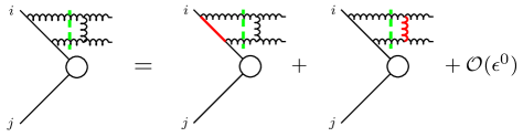
Figure 9: Schematic representation of regions that give rise to infrared poles. Poles arise as a result of the vanishing of the red propagators.

In general the integrals of these cut graphs contain more than one region in which the propagators vanish and, in dimensional regularization, each region gives rise to a $1/\epsilon$ pole. To illustrate the point, we consider the first cut graph in Fig. 9, which gives

$$\frac{1}{2}\mathbb{T}_{i}^{a}if^{ac_{2}b}if^{bc_{1}d}\mathbb{T}_{i}^{d}\int\frac{\text{d}^{d}l}{(2\pi)^{d}}\frac{if(l,p_{i},q_{1},q_{2})\,(2\pi)\delta^{+}(l)\,(2\pi)\delta^{+}(q_{1}+q_{2}-l)}{(p_{i}\cdot l)(l\cdot q_{1})}\,,$$ (47)

where $f$ is a scalar function whose precise form is not important and $\delta^{+}(l)=\theta(l_{0})\delta(l^{2})$. In the reference frame in which the time-like vector $q_{1}+q_{2}$ is at rest, one can integrate over the energy $l_{0}$ and the magnitude of the $(d-1)$-momentum $|\vec{l}|$ to give

$$\frac{1}{2}\mathbb{T}_{i}^{a}if^{ac_{2}b}if^{bc_{1}d}\mathbb{T}_{i}^{d}\,\frac{((q_{1}^{0}+q_{2}^{0})/2)^{d-6}}{8(2\pi)^{d-2}p_{i}^{0}q_{1}^{0}}\int\text{d}\Omega_{d-2}\frac{if(l)}{[1-\hat{p}_{i}\cdot\hat{l}][1-\hat{q}_{1}\cdot\hat{l}]}\,,$$ (48)

where $\text{d}\Omega_{d-2}$ is the solid angle element of the unit $(d-2)$-sphere. Clearly the denominator of the integrand only vanishes when the virtual light-like momentum is either collinear with $p_{i}$ or $q_{1}$, which cannot occur simultaneously. It follows that the pole part of this expression can be computed as

$$\int\text{d}\Omega_{d-2}\frac{f(l)}{[1-\hat{p}_{i}\cdot\hat{l}][1-\hat{q}_{1}\cdot\hat{l}]} = \frac{f(l)|_{\hat{l}=\hat{p}_{i}}}{1-\hat{p}_{i}\cdot\hat{q}_{1}}\int\frac{\text{d}\Omega_{d-2}}{[1-\hat{p}_{i}\cdot\hat{l}]}$$ (49)

$$+ \frac{f(l)|_{\hat{l}=\hat{q}_{1}}}{1-\hat{p}_{i}\cdot\hat{q}_{1}}\int\frac{\text{d}\Omega_{d-2}}{[1-\hat{q}_{1}\cdot\hat{l}]}+\mathcal{O}(\epsilon^{0}).$$

The remaining angular integration can be performed by standard methods, after which, Eq. (47) can be written

$$\mathbb{T}_{i}^{a}if^{ac_{2}b}if^{bc_{1}d}\mathbb{T}_{i}^{d}\,\frac{-i\pi}{8\pi^{2}}\frac{1}{(-p_{i}\cdot q_{1})(q_{1}+q_{2})^{2}}\left[-\frac{f(l)}{\epsilon}\Bigg{|}_{l=\frac{q_{1}\cdot q_{2}}{p_{i}\cdot(q_{1}+q_{2})}p_{i}}-\frac{f(l)}{\epsilon}\Bigg{|}_{l=q_{1}}\right]+\mathcal{O}(\epsilon^{0}).$$ (50)

This expression indicates that the pole part of this cut graph arises from the region in which the virtual emission is collinear to the hard momentum $l^{\mu}\to\frac{q_{1}\cdot q_{2}}{p_{i}\cdot(q_{1}+q_{2})}p_{i}^{\mu}$ and from the collinear region $l^{\mu}\to q_{1}^{\mu}$. The latter corresponds to an infinitely soft virtual exchange between the two real emissions. These two contributions are represented on the right-hand side of Fig. 9.

Exactly the same type of analysis can be carried out to compute the pole parts of each of the cut graphs in Fig. 8. In all cases, the $1/\epsilon$ poles arise either from the region in which one of the eikonal propagators vanishes (collinear singularities) or from the region in which the two real emissions exchange a soft gluon between them. We note that included in Fig. 8 are cut self-energy graphs and the corresponding ghost graphs should be added to these. However, neither of them gives rise to infrared poles (or their associated logarithms).

The colour operator associated with each leading graph in Fig. 8 can be written as a linear combination of the colour structure on the left-hand side of Fig. 10 and its permutation $(1\leftrightarrow 2)$. For example, the colour operator corresponding to the graph in Fig. 9 can be rewritten as

$$\mathbb{T}_{i}^{a}if^{ac_{2}b}if^{bc_{1}d}\mathbb{T}_{i}^{d}\Bigl{|}M^{(0)}\Bigr{\rangle}=-\mathbb{T}_{j}^{d}if^{dc_{1}b}if^{bc_{2}a}\mathbb{T}_{i}^{a}\Bigl{|}M^{(0)}\Bigr{\rangle}~{}.$$ (51)

After expressing all of the colour structures in this way, one can confirm that the poles corresponding to collinear singularities cancel. This cancellation gives rise to the zero on the right-hand side of Fig. 10.

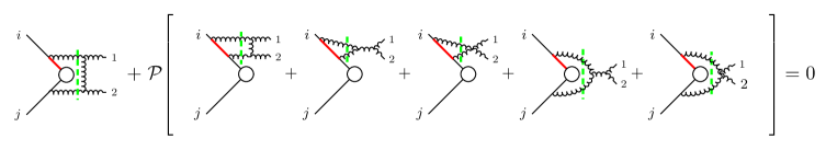
Figure 10: Cancellation of collinear poles. The operator $\mathcal{P}$ projects out the appropriate colour structure.

It follows that the only $1/\epsilon$ poles of the cut graphs in Fig. 8 arise from a Coulomb exchange between the two real emissions. These are represented in Fig. 11.

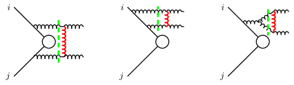
Figure 11: The relevant $1/\epsilon$ poles arising from soft-gluon cuts correspond to Coulomb exchange between the two real emissions.

Explicitly, the pole part of the amplitude arising from the sum over all soft gluon cuts can written

$$-\frac{1}{\epsilon}\left[\frac{-i\pi}{8\pi^{2}}if^{c_{1}ea_{1}}if^{c_{2}ea_{2}}\right]\mathbb{K}_{2}^{a_{1}a_{2}}(q_{1},q_{2})\Bigl{|}M^{(0)}\Bigr{\rangle},$$ (52)

where $\mathbb{K}_{2}(q_{1},q_{2})$ is the two-gluon emission tensor. This expression can be combined with the pole part of Eq. (44) to determine the leading $1/\epsilon$ pole of the imaginary part of the double-emission amplitude.

We will now go beyond the calculation of the leading $\epsilon$ poles and compute the corresponding leading logarithmic contribution arising from the soft gluon cuts. As before we will compute all of the contributing Feynman graphs exactly in dimensional regularisation and within the eikonal approximation, and then extract the leading behaviour in limits 1–3. To do this we make use of Ellis:2011cr ; Huber:2007dx ; vanNeerven . Recall that the colour part of all of the graphs can be written as a linear combination of the colour structure of the graph on the left-hand side of Fig. 10 and its permutation $(1\leftrightarrow 2)$. Written in terms of these two colour tensors, in limit 1, the amplitude is

$$- \frac{i\pi}{8\pi^{2}}\left[\frac{p_{j}\cdot\varepsilon_{1}}{p_{j}\cdot q_{1}}-\frac{p_{i}\cdot\varepsilon_{1}}{p_{i}\cdot q_{1}}\right]\left\{\left[\frac{p_{j}\cdot\varepsilon_{2}}{p_{j}\cdot q_{2}}-\frac{q_{1}\cdot\varepsilon_{2}}{q_{1}\cdot q_{2}}\right]\left[-\frac{1}{\epsilon}+\ln\left(\frac{2q_{2}\cdot q_{1}\,p_{j}\cdot q_{2}}{q_{1}\cdot p_{j}\;\mu^{2}}\right)\right]\mathbb{T}_{j}^{d}if^{dc_{2}b}if^{bc_{1}a}\mathbb{T}_{i}^{a}\right.$$ (53)

$$- \left.\left[\frac{p_{i}\cdot\varepsilon_{2}}{p_{i}\cdot q_{2}}-\frac{q_{1}\cdot\varepsilon_{2}}{q_{1}\cdot q_{2}}\right]\left[-\frac{1}{\epsilon}+\ln\left(\frac{2q_{2}\cdot q_{1}\,p_{i}\cdot q_{2}}{q_{1}\cdot p_{i}\;\mu^{2}}\right)\right]\mathbb{T}_{j}^{d}if^{dc_{1}b}if^{bc_{2}a}\mathbb{T}_{i}^{a}\right\}\Bigl{|}M^{0}\Bigr{\rangle}~{}.$$

This expression is manifestly gauge invariant but, at first sight, it looks quite different from Eq. (52). As we will discuss in more detail in the next section, each of the logarithmic terms can be written in terms of the transverse momentum of gluon 2 measured in either the $p_{j}\!+\!q_{1}$ or $p_{i}\!+\!q_{1}$ rest frame:

$$q_{2T(i1)}^{2}=\frac{2q_{2}\cdot q_{1}\,p_{i}\cdot q_{2}}{q_{1}\cdot p_{i}}\,.$$ (54)

In order to compare Eq. (53) with Eq. (52), it is convenient to introduce the rapidity:

$$q^{\pm}_{i}=q_{iT}e^{\pm y_{i}}/\sqrt{2}~{}.$$ (55)

The logarithms are then

$$\ln\left(\frac{2q_{2}\cdot q_{1}\,p_{i}\cdot q_{2}}{q_{1}\cdot p_{i}\mu^{2}}\right)=\ln\left(\frac{q_{2T(i1)}^{2}}{\mu^{2}}\right)=\ln\left(\frac{q_{2T}^{2}}{\mu^{2}}\right)+\ln\left(\frac{2q_{1}\cdot q_{2}}{q_{1T}{q_{2T}}}\right)+y_{1}-y_{2},$$ (56)

$$\ln\left(\frac{2q_{2}\cdot q_{1}\,p_{j}\cdot q_{2}}{q_{1}\cdot p_{j}\mu^{2}}\right)=\ln\left(\frac{q_{2T(j1)}^{2}}{\mu^{2}}\right)=\ln\left(\frac{q_{2T}^{2}}{\mu^{2}}\right)+\ln\left(\frac{2q_{1}\cdot q_{2}}{q_{1T}{q_{2T}}}\right)+y_{2}-y_{1},$$ (57)

and we see that the two are equal up to formally sub-leading terms ($\propto y_{i}$). Eq. (53) can therefore be simplified and, using colour conservation and the colour algebra, written as

$$\left\{-\frac{i\pi}{8\pi^{2}}if^{c_{1}ea_{1}}if^{c_{2}ea_{2}}\left[-\frac{1}{\epsilon}+\ln\left(\frac{q_{2T}^{2}}{\mu^{2}}\right)+\ln\left(\frac{2q_{1}\cdot q_{2}}{q_{1T}{q_{2T}}}\right)\right]\right\}\;\mathbb{K}_{2}^{a_{1}a_{2}}(q_{1},q_{2})\Bigl{|}M^{(0)}\Bigr{\rangle}~{}.$$ (58)

The operator enclosed in curly brackets has the colour structure of a Coulomb exchange between the two soft real emissions, and its pole part agrees with Eq. (52). The first logarithm can be written as

$$-\frac{1}{\epsilon}+\ln\left(\frac{q_{2T}^{2}}{\mu^{2}}\right)+\mathcal{O}(\epsilon)=\int_{0}^{q_{2T}^{2}}\frac{\mu^{2\epsilon}\;\text{d}l_{T}^{2}}{(l_{T}^{2})^{1+\epsilon}},$$ (59)

which is in agreement with Eq. (1), and the second logarithm is sub-leading.

In limits 2 and 3, the sum over soft gluon cuts can be written as

$$\left\{-\frac{i\pi}{8\pi^{2}}if^{c_{1}ea_{1}}if^{c_{2}ea_{2}}\int^{q_{2T}^{2}}_{0}\frac{\mu^{2\epsilon}\;\text{d}l_{T}^{2}}{(l_{T}^{2})^{1+\epsilon}}\right\}\mathbb{K}_{2}^{a_{1}a_{2}}(q_{1},q_{2})\Bigl{|}M^{(0)}\Bigr{\rangle}~{}.$$ (60)

Once again, the result in limits 2 and 3 can be deduced by taking the corresponding collinear limit of the leading expression in limit 1, Eq. (53).

The leading cuts in limits 1–3 are presented in Fig. 12 and can be expressed in terms of the two colour tensors in Eq. (53), which are illustrated in the final column of the figure. There are additional graphs, other than the ones shown, that involve the four-gluon vertex but, along with the ghost graphs, these are sub-leading.

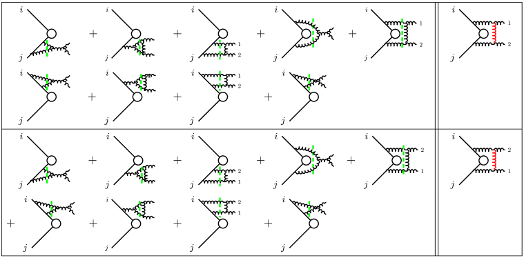
Figure 12: Leading graphs in limits 1–3. Their contributions are projected onto the two colour structures in the final column.

In limit 1 all cuts in this figure are leading except that with a four-gluon vertex. The non-trivial way in which these graphs combine to deliver Eq. (53) is illustrated by considering, as an example, the graphs that give rise to the term with Lorentz structure

$$-\frac{i\pi}{8\pi^{2}}\frac{p_{j}\cdot\varepsilon_{1}}{p_{j}\cdot q_{1}}\frac{q_{1}\cdot\varepsilon_{2}}{q_{1}\cdot q_{2}}$$ (61)

in the first line of Eq. (53). The first five graphs of each colour structure are all leading. In the case of the first colour structure (the top half of Fig. 12) we label these $\{G_{1a},G_{1b},G_{1c},G_{1d},G_{1e}\}$. The first two of these cancel exactly, whilst the others give

$$G_{1c} = -\frac{3}{2}\int_{p_{j}\cdot q_{1}}^{p_{j}\cdot q_{2}}\frac{\text{d}l_{T}^{2}}{l_{T}^{2}}-\frac{3}{2}\int_{0}^{2q_{1}\cdot q_{2}}\frac{\text{d}l_{T}^{2}}{l_{T}^{2}},$$ (62)

$$G_{1d} = \frac{3}{2}\int_{0}^{2q_{1}\cdot q_{2}}\frac{\text{d}l_{T}^{2}}{l_{T}^{2}},$$ (63)

$$G_{1e} = -\int_{0}^{2q_{1}\cdot q_{2}}\frac{\text{d}l_{T}^{2}}{l_{T}^{2}}+\frac{1}{2}\int^{p_{j}\cdot q_{2}}_{p_{j}\cdot q_{1}}\frac{\text{d}l_{T}^{2}}{l_{T}^{2}}.$$ (64)

In stark contrast, for the second colour structure the first two graphs again cancel exactly but the others now give

$$G_{2c} = \frac{3}{4}\int_{0}^{2q_{1}\cdot q_{2}}\frac{\text{d}l_{T}^{2}}{l_{T}^{2}},$$ (65)

$$G_{2d} = -\frac{3}{2}\int_{0}^{2q_{1}\cdot q_{2}}\frac{\text{d}l_{T}^{2}}{l_{T}^{2}},$$ (66)

$$G_{2e} = \frac{7}{4}\int_{0}^{2q_{1}\cdot q_{2}}\frac{\text{d}l_{T}^{2}}{l_{T}^{2}}+\int^{p_{i}\cdot q_{2}}_{p_{i}\cdot q_{1}}\frac{\text{d}l_{T}^{2}}{l_{T}^{2}}.$$ (67)

In both cases, these terms sum up to give the corresponding terms in Eq. (53).

Limit 2 is particularly simple since from all the graphs in Figure 12 only graphs $G_{2e}$ and $G_{2h}$ are leading and they give rise to the two terms

$$-\frac{i\pi}{8\pi^{2}}\frac{1}{2}\frac{p_{i}\cdot\varepsilon_{2}}{p_{i}\cdot q_{2}}\frac{p_{i}\cdot\varepsilon_{1}}{p_{i}\cdot q_{1}}\int_{0}^{q_{2T}^{2}}\frac{\text{d}l_{T}^{2}}{l_{T}^{2}}$$ (68)

and

$$-\frac{i\pi}{8\pi^{2}}\left[\frac{1}{2}\frac{p_{i}\cdot\varepsilon_{2}}{p_{i}\cdot q_{2}}\frac{p_{i}\cdot\varepsilon_{1}}{p_{i}\cdot q_{1}}-\frac{p_{i}\cdot\varepsilon_{2}}{p_{i}\cdot q_{2}}\frac{p_{j}\cdot\varepsilon_{1}}{p_{j}\cdot q_{1}}\right]\int_{0}^{q_{2T}^{2}}\frac{\text{d}l_{T}^{2}}{l_{T}^{2}}~{},$$ (69)

which add up to the corresponding collinear limit of Eq. (53).

Finally we study the leading cuts in limit 3. There are leading contributions to the second colour structure but they cancel. The first colour structure receives leading contributions to the following two Lorentz structures:

$$-\frac{i\pi}{8\pi^{2}}\left\{\frac{\varepsilon_{1}^{-}}{q_{1}^{-}}\frac{\varepsilon_{2}^{+}}{q_{2}^{+}},\frac{\varepsilon_{1}^{-}}{q_{1}^{-}}\frac{\varepsilon_{2}^{-}}{q_{2}^{-}}\right\}~{}.$$ (70)

Only graph $G_{1e}$ contributes to the first and it gives

$$-\int_{0}^{q_{2T}^{2}}\frac{\text{d}l_{T}^{2}}{l_{T}^{2}}.$$ (71)

Graphs $\{G_{1a},G_{1b},G_{1c},G_{1d},G_{1e},G_{1i}\}$ contribute to the second Lorentz structure in (70). The contributions of graphs $G_{1a},G_{1b}$ cancel whilst

$$G_{1c} = \left[\frac{3(q_{1}^{-})^{2}+3q_{1}^{-}q_{2}^{-}+2(q_{2}^{-})^{2}}{4(q_{1}^{-}+q_{2}^{-})^{2}}\right]\int_{0}^{q_{1}^{+}q_{2}^{-}}\frac{\text{d}l_{T}^{2}}{l_{T}^{2}}-\frac{1}{2}\int_{p_{i}\cdot q_{1}}^{p_{i}\cdot(q_{1}+q_{2})}\frac{\text{d}l_{T}^{2}}{l_{T}^{2}},$$ (72)

$$G_{1d} = -\frac{3q_{1}^{-}+2q_{2}^{-}}{2(q_{1}^{-}+q_{2}^{-})}\int_{0}^{q_{1}^{+}q_{2}^{-}}\frac{\text{d}l_{T}^{2}}{l_{T}^{2}}+\int_{p_{i}\cdot q_{1}}^{p_{i}\cdot(q_{1}+q_{2})}\frac{dl_{T}^{2}}{l_{T}^{2}},$$ (73)

$$G_{1e} = \frac{7q_{1}^{-}+6q_{2}^{-}}{4(q_{1}^{-}+q_{2}^{-})}\int_{0}^{q_{1}^{+}q_{2}^{-}}\frac{\text{d}l_{T}^{2}}{l_{T}^{2}}-\frac{1}{2}\int_{p_{i}\cdot q_{1}}^{p_{i}\cdot(q_{1}+q_{2})}\frac{\text{d}l_{T}^{2}}{l_{T}^{2}}-\int^{p_{j}\cdot q_{1}}_{p_{j}\cdot q_{2}}\frac{\text{d}l_{T}^{2}}{l_{T}^{2}}.$$ (74)

The sum of these three contributions is

$$\int_{0}^{q_{2T}^{2}}\frac{\text{d}l_{T}^{2}}{l_{T}^{2}}-\frac{q_{1}^{-}q_{2}^{-}}{2(q_{1}^{-}+q_{2}^{-})^{2}}\int_{0}^{q_{1}^{+}q_{2}^{-}}\frac{\text{d}l_{T}^{2}}{l_{T}^{2}}~{}.$$ (75)

Finally, the four-gluon vertex graph $G_{1i}$ exactly cancels the second term of this expression and so the sum of leading graphs in limit 3 reduces to

$$-\frac{i\pi}{8\pi^{2}}\frac{\varepsilon_{1}^{-}}{q_{1}^{-}}\left[\frac{\varepsilon_{2}^{-}}{q_{2}^{-}}-\frac{\varepsilon_{2}^{+}}{q_{2}^{+}}\right]\int_{0}^{q_{2T}^{2}}\frac{\text{d}l_{T}^{2}}{l_{T}^{2}}\mathbb{T}_{j}^{d}if^{dc_{2}b}if^{bc_{1}a}\mathbb{T}_{i}^{a}.$$ (76)

This expression is identical to the corresponding collinear limit of Eq. (53).

It is clear that while the sum of diagrams reproduces $k_{T}$ ordering in all three limits, the contributions of individual diagrams are very different in each region. In particular, the emergence of $k_{T}$ ordering in limit 3, of most importance for the understanding of super-leading logarithms and factorization breaking, involves a very non-trivial interplay of many different orderings in many different individual diagrams (in Feynman gauge at least).

4.4 Physical picture

In this section, we re-derive the result of the previous section, in a way that emphasises its physical interpretation. The final result will be identical to Eq. (53), but it will be clear that this represents a $k_{T}$ ordering in a dipole-like picture: the lower-$k_{T}$ gluon is emitted by a dipole formed by the higher-$k_{T}$ gluon and one of the hard partons, and the $k_{T}$ of the exchanged Coulomb gluon is limited by the local transverse momentum of the softer gluon, in the frame defined by the dipole of its emission. It is this local transverse momentum, which is different for different dipoles, that appears in the logarithms in Eq. (53).

We consider a general form of the one-loop amplitude to produce two soft gluons. In particular, we want to calculate the contribution to the imaginary part of that amplitude coming from diagrams in which two gluons (or ghosts) are produced at tree-level and scatter to produce the final-state gluons. Suppressing the colour indices, we may write this amplitude as

$$i\mathcal{M}=\int\frac{\mathrm{d}^{d-2}k_{T}}{8q_{1}\!\cdot\!q_{2}(2\pi)^{d-2}\sqrt{1-2k_{T}^{2}/(q_{1}\!\cdot\!q_{2})}}\times\frac{1}{2}(i\mathcal{A}^{\mu\nu})\Biggl{(}\sum_{p_{1}^{\prime}}\varepsilon^{*}_{1^{\prime}\mu;p_{1}^{\prime}}\varepsilon_{1^{\prime}\sigma;p_{1}^{\prime}}\sum_{p_{2}^{\prime}}\varepsilon^{*}_{2^{\prime}\nu;p_{2}^{\prime}}\varepsilon_{2^{\prime}\lambda;p_{2}^{\prime}}\Biggr{)}(i\mathcal{B}^{\sigma\lambda})~{},$$ (77)

where $\mathcal{A}$ is the amplitude to produce a pair of gluons with momenta $q_{1}^{\prime}$ and $q_{2}^{\prime}$ and $\mathcal{B}$ is the amplitude for that same pair of gluons to scatter into the two final state gluons with momenta $q_{1}$ and $q_{2}$. The integration variable $k$ is defined by $q_{1}^{\prime}=q_{1}+k$ and $q_{2}^{\prime}=q_{2}-k$, and the polarization sums are over physical (on-shell) polarizations of the cut gluons (labelled by $p_{1}^{\prime}$ and $p_{2}^{\prime}$).

We will see that our interest is in the region $k_{T}^{2}\ll 2q_{1}\!\cdot\!q_{2}$. In this case, and with physical polarizations for the gluons, $\mathcal{B}$ is dominated by the $t$-channel diagram:

$$\varepsilon_{1^{\prime}\sigma;p_{1}^{\prime}}\varepsilon_{2^{\prime}\lambda;p_{2}^{\prime}}\mathcal{B}^{\sigma\lambda}\stackrel{{\scriptstyle k_{T}^{2}\ll 2q_{1}\cdot q_{2}}}{{\longrightarrow}}g_{s}^{2}\mu^{2\epsilon}\,\frac{4q_{1}\!\cdot\!q_{2}}{k_{T}^{2}}\,\varepsilon_{1^{\prime};p_{1}^{\prime}}\!\cdot\!\varepsilon^{*}_{1;p_{1}}\,\varepsilon_{2^{\prime};p_{2}^{\prime}}\!\cdot\!\varepsilon^{*}_{2;p_{2}}\,,$$ (78)

where $p_{1,2}$ label the polarization states of the outgoing gluons. Therefore we have

$$\mathcal{M}=\frac{ig_{s}^{2}\mu^{2\epsilon}}{8\pi^{2}}\int\frac{\mathrm{d}^{d-2}k_{T}}{k_{T}^{2}(2\pi)^{d-4}}\sum_{p_{1}^{\prime}p_{2}^{\prime}}\Biggl{(}\mathcal{A}^{\mu\nu}\varepsilon^{*}_{1^{\prime}\mu;p_{1}^{\prime}}\varepsilon^{*}_{2^{\prime}\nu;p_{2}^{\prime}}\Biggr{)}\varepsilon_{1^{\prime};p_{1}^{\prime}}\!\cdot\!\varepsilon^{*}_{1;p_{1}}\,\varepsilon_{2^{\prime};p_{2}^{\prime}}\!\cdot\!\varepsilon^{*}_{2;p_{2}}\,.$$ (79)

When $k_{T}$ is extremely small, the polarization vector dot-products become diagonal, i.e. $\varepsilon_{1^{\prime};p_{1}^{\prime}}\!\cdot\!\varepsilon^{*}_{1;p_{1}}\to-\delta_{p_{1}^{\prime}p_{1}}$, the momenta $q^{\prime}_{1,2}$ become $q_{1,2}$ and there is a complete factorization of the production, $\mathcal{A}^{\mu\nu}\varepsilon^{*}_{1\mu;p_{1}}\varepsilon^{*}_{2\nu;p_{2}}$, from the scattering. However, $k_{T}^{2}\ll 2q_{1}\!\cdot\!q_{2}$ is not a sufficient condition for this and we must evaluate the polarization vector dot-products more accurately.

Limit 1

In limit 1 (i.e. the keeping the leading-$\lambda$ terms after the rescaling $q_{2}\to\lambda q_{2}$), $\mathcal{A}^{\mu\nu}$ is a sum of terms each of which has a different colour factor, and has the form

$$\mathcal{A}^{\mu\nu}\sim\mathcal{A}^{\mu}\left(\frac{p_{i}^{\nu}}{p_{i}\!\cdot\!q_{2}}-\frac{q_{1}^{\nu}}{q_{1}\!\cdot\!q_{2}}\right),$$ (80)

where $p_{i}$ is one of the (fast) eikonal-line momenta. We will find that the region of interest is $k_{T}^{2}\;\raisebox{-1.72218pt}{\hbox to0.0pt{$\sim$\hss}}\raisebox{1.72218pt}{$<$}\;2\,p_{i}\!\cdot\!q_{2}\,q_{1}\!\cdot\!q_{2}/p_{i}\!\cdot\!q_{1}\sim\lambda^{2}$, so $k_{T}$ can also be taken to obey the scaling $k_{T}\to\lambda k_{T}$.

In order to evaluate the integral in Eq. (79), we construct explicit representations of the polarization vectors. The polarization vectors for $q^{\prime}_{1,2}$ are both perpendicular to both $q^{\prime}_{1}$ and $q^{\prime}_{2}$. Obviously the space of such vectors is 2-dimensional and we can choose basis vectors that span it. To do so, we need an additional vector, to define the plane of zero azimuth. With an eye on the structure of Eq. (80), we use $p_{i}$ to define this frame. That is, we take as our polarization vectors

$$\varepsilon_{1^{\prime}\mu;\perp} = \epsilon_{\mu\nu\lambda\sigma}q^{\prime\nu}_{1}q^{\prime\lambda}_{2}p_{i}^{\sigma}\,\frac{1}{\sqrt{2\,p_{i}\!\cdot\!q^{\prime}_{1}\,p_{i}\!\cdot\!q^{\prime}_{2}\,q^{\prime}_{1}\!\cdot\!q^{\prime}_{2}}}\,,$$ (81)

$$\varepsilon_{2^{\prime}\mu;\perp} = \epsilon_{\mu\nu\lambda\sigma}q^{\prime\nu}_{2}q^{\prime\lambda}_{1}p_{i}^{\sigma}\,\frac{1}{\sqrt{2\,p_{i}\!\cdot\!q^{\prime}_{1}\,p_{i}\!\cdot\!q^{\prime}_{2}\,q^{\prime}_{1}\!\cdot\!q^{\prime}_{2}}}\,,$$ (82)

which are perpendicular to the plane that contains $q^{\prime}_{1}$, $q^{\prime}_{2}$ and $p_{i}$ in the $q^{\prime}_{1}\!+\!q^{\prime}_{2}$ rest frame, and

$$\varepsilon_{1^{\prime}\mu;\parallel} = \biggl{(}q^{\prime}_{1}\!\cdot\!q^{\prime}_{2}\,p_{i\mu}-p_{i}\!\cdot\!q^{\prime}_{1}\,q^{\prime}_{2\mu}-p_{i}\!\cdot\!q^{\prime}_{2}\,q^{\prime}_{1\mu}\biggr{)}\,\frac{1}{\sqrt{2\,p_{i}\!\cdot\!q^{\prime}_{1}\,p_{i}\!\cdot\!q^{\prime}_{2}\,q^{\prime}_{1}\!\cdot\!q^{\prime}_{2}}}\,,$$ (83)

$$\varepsilon_{2^{\prime}\mu;\parallel} = \biggl{(}q^{\prime}_{1}\!\cdot\!q^{\prime}_{2}\,p_{i\mu}-p_{i}\!\cdot\!q^{\prime}_{2}\,q^{\prime}_{1\mu}-p_{i}\!\cdot\!q^{\prime}_{1}\,q^{\prime}_{2\mu}\biggr{)}\,\frac{1}{\sqrt{2\,p_{i}\!\cdot\!q^{\prime}_{1}\,p_{i}\!\cdot\!q^{\prime}_{2}\,q^{\prime}_{1}\!\cdot\!q^{\prime}_{2}}}\,,$$ (84)

which are in that plane. It is worth noting that these statements are also true in the $p_{i}\!+\!q^{\prime}_{1}$ rest frame: $\perp$ and $\parallel$ states are perpendicular to and in the plane of emission of $q^{\prime}_{2}$ in that frame. We also define polarization vectors for the gluons with unprimed momenta in the exactly analogous way. Since the $q_{1}\!+\!q_{2}$ rest frame is also the $q^{\prime}_{1}\!+\!q^{\prime}_{2}$ rest frame, the two sets of polarization vectors are related only by rotations.

According to the definition of $k$ above and the fact that two of its components have been integrated out to put the intermediate gluons on shell, we have

$$q^{\prime}_{1} = (1-\beta)q_{1}+\beta q_{2}+k_{T}\approx q_{1},$$ (85)

$$q^{\prime}_{2} = (1-\beta)q_{2}+\beta q_{1}-k_{T}\approx q_{2}+\frac{k_{T}^{2}}{2q_{1}\!\cdot\!q_{2}}q_{1}-k_{T},$$ (86)

$$\beta = \frac{1}{2}\left(1-\sqrt{1-\frac{2k_{T}^{2}}{q_{1}\!\cdot\!q_{2}}}\right)\approx\frac{k_{T}^{2}}{2q_{1}\!\cdot\!q_{2}}\,,$$ (87)

where, in each case, the first result is exact, while the second is in the leading-$\lambda$ approximation.

Turning to the polarization vectors in Eq. (79), we first consider the gluon-1 line. We have

$$\sum_{p_{1}^{\prime}}\mathcal{A}^{\mu}\varepsilon^{*}_{1^{\prime}\mu;p_{1}^{\prime}}\,\varepsilon_{1^{\prime};p_{1}^{\prime}}\!\cdot\!\varepsilon^{*}_{1;p_{1}}\,.$$ (88)

If $\varepsilon^{*}_{1;p_{1}}$ lies in the space spanned by $\varepsilon_{1^{\prime};p_{1}^{\prime}}$, then this becomes a completeness relation and trivial. Counting powers of $\lambda$ in all terms, we can show that this is the case in all of limits 1, 2 and 3, and we can write

$$\sum_{p_{1}^{\prime}}\mathcal{A}^{\mu}\varepsilon^{*}_{1^{\prime}\mu;p_{1}^{\prime}}\,\varepsilon_{1^{\prime};p_{1}^{\prime}}\!\cdot\!\varepsilon^{*}_{1;p_{1}}=-\mathcal{A}^{\mu}\varepsilon^{*}_{1\mu;p_{1}}\,.$$ (89)

That is, in the leading-$\lambda$ approximation, we can take gluon 1’s momentum and polarization state as being unchanged by the Coulomb scattering.

Making the same analysis for gluon 2, we find that the polarization sum is not complete (or rather, the polarization vector $\varepsilon^{*}_{2;p_{2}}$ does not lie in the space spanned by $\varepsilon_{2^{\prime};p_{2}^{\prime}}$) and therefore we have to evaluate the dot-product explicitly. Physically, this corresponds to the fact that, although the scattering is soft, gluon 2 is so much softer than gluon 1 that the small fraction of gluon 1’s momentum that is transferred to gluon 2 does change its momentum and polarization state significantly.

That is, we have to calculate

$$\mathcal{M}=-\frac{ig_{s}^{2}\mu^{2\epsilon}}{8\pi^{2}}\int\frac{\mathrm{d}^{d-2}k_{T}}{k_{T}^{2}(2\pi)^{d-4}}\sum_{p_{2}^{\prime}}\Biggl{(}\mathcal{A}^{\mu\nu}\varepsilon^{*}_{1\mu;p_{1}}\,\varepsilon^{*}_{2^{\prime}\nu;p_{2}^{\prime}}\Biggr{)}\varepsilon_{2^{\prime};p_{2}^{\prime}}\!\cdot\!\varepsilon^{*}_{2;p_{2}}.$$ (90)

To do this, we construct an explicit $k_{T}$ vector. Since $q_{1,2}$ and $p_{i}$ stay fixed during the $k_{T}$ integration, $\varepsilon_{1\mu;\perp}$ and $\varepsilon_{1\mu;\parallel}$ are appropriate unit vectors perpendicular to $q_{1,2}$ and we can write

$$k_{T\mu}=k_{T}\sin\phi\,\varepsilon_{1\mu;\perp}+k_{T}\cos\phi\,\varepsilon_{1\mu;\parallel}\,.$$ (91)

We also note that the dipole form in Eq. (80) does not couple to gluons polarized out of the plane and hence the sum over polarizations $p_{2}^{\prime}$ is only over $p_{2}^{\prime}=\parallel$. By explicit calculation, we find that all contributions integrate to zero, except for diagonal scattering of an in-plane polarized gluon scattering to an in-plane polarized gluon yielding a contribution to the amplitude of

$$\left(\frac{p_{i}^{\nu}}{p_{i}\cdot q^{\prime}_{2}}-\frac{q_{1}^{\nu}}{q_{1}\cdot q_{2}^{\prime}}\right)\varepsilon^{*}_{2^{\prime}\nu;\parallel}\,\varepsilon_{2^{\prime};\parallel}\cdot\varepsilon_{2;\parallel}^{*} = -\left(\frac{p_{i}^{\nu}}{p_{i}\cdot q_{2}}-\frac{q_{1}^{\nu}}{q_{1}\cdot q_{2}}\right)\varepsilon^{*}_{2\nu;\parallel}\,$$ (92)

$$\times\frac{1+k_{T}\cos\phi\sqrt{\frac{p_{i}\cdot q_{1}}{2\,p_{i}\cdot q_{2}\,q_{1}\cdot q_{2}}}}{1+2k_{T}\cos\phi\sqrt{\frac{p_{i}\cdot q_{1}}{2\,p_{i}\cdot q_{2}\,q_{1}\cdot q_{2}}}+k_{T}^{2}\frac{p_{i}\cdot q_{1}}{2\,p_{i}\cdot q_{2}\,q_{1}\cdot q_{2}}}\,,$$

where $\phi=0$ is given by the plane containing $p_{i}$. Note that this expression is a function only of $k_{T}/q_{2T(i1)}$, where

$$q_{2T(i1)}^{2}=\frac{2\,p_{i}\cdot q_{2}\,q_{1}\cdot q_{2}}{p_{i}\cdot q_{1}}$$ (93)

is the transverse momentum of gluon 2 in the $p_{i}\!+\!q_{1}$ rest frame.

Putting everything together we have

$$\mathcal{M}=\Biggl{(}\mathcal{A}^{\mu\nu}\varepsilon^{*}_{1\mu;p_{1}}\,\varepsilon^{*}_{2\nu;p_{2}}\Biggr{)}\frac{ig_{s}^{2}\mu^{2\epsilon}}{8\pi^{2}}\int\frac{k_{T}^{d-3}\mathrm{d}k_{T}\,\mathrm{d}\phi\,\sin^{-2\epsilon}\phi\,\mathrm{d}^{d-4}\Omega}{k_{T}^{2}(2\pi)^{d-4}}\,\frac{1+\frac{k_{T}}{q_{2T(i1)}}\cos\phi}{1+2\frac{k_{T}}{q_{2T(i1)}}\cos\phi+\frac{k_{T}^{2}}{q_{2T(i1)}^{2}}}\,.$$ (94)

The integral can be performed exactly in $d$ dimensions and is

$$\mathcal{M}=\Biggl{(}\mathcal{A}^{\mu\nu}\varepsilon^{*}_{1\mu;p_{1}}\,\varepsilon^{*}_{2\nu;p_{2}}\Biggr{)}i\pi\,\frac{\alpha_{s}}{2\pi}\,\frac{\Gamma(1-\epsilon)^{2}\Gamma(1+\epsilon)}{\Gamma(1-2\epsilon)}\left(\frac{4\pi\mu^{2}}{q_{2T(i1)}^{2}}\right)^{\epsilon}\left(-\frac{1}{\epsilon}\right)\,,$$ (95)

which we have confirmed is in exact agreement with the full calculation from the sum over all diagrams.

To illustrate the physical structure, it is better to move to four dimensions where, remarkably, the $\phi$ integral yields an exact $\Theta$-function:

$$\mathcal{M}=\Biggl{(}\mathcal{A}^{\mu\nu}\varepsilon^{*}_{1\mu;p_{1}}\,\varepsilon^{*}_{2\nu;p_{2}}\Biggr{)}\frac{ig_{s}^{2}}{4\pi}\,\int_{0}^{q_{2T(i1)}}\frac{\mathrm{d}k_{T}}{k_{T}}\,.$$ (96)

That is, the $k_{T}$ of the Coulomb gluon is exactly limited by the transverse momentum of the softer of the two gluons it is exchanged between, as measured in the rest frame of a dipole formed by the harder of the two gluons and one of the fast partons in the hard process.

In deriving Eq. (96), we assumed that $\mathcal{A}^{\mu\nu}$ has the form of a dipole emission for the emission of gluon 2 in limit 1. This is, quite generally, the case. In the particular case of two coloured partons annihilating into a colourless system, which we consider in most of this paper, we can explicitly write the final result as

$$- \frac{i\pi}{8\pi^{2}}\left[\frac{p_{j}\cdot\varepsilon_{1}}{p_{j}\cdot q_{1}}-\frac{p_{i}\cdot\varepsilon_{1}}{p_{i}\cdot q_{1}}\right]\left\{\left[\frac{p_{j}\cdot\varepsilon_{2}}{p_{j}\cdot q_{2}}-\frac{q_{1}\cdot\varepsilon_{2}}{q_{1}\cdot q_{2}}\right]\int_{0}^{\frac{2q_{2}\cdot q_{1}\,p_{j}\cdot q_{2}}{q_{1}\cdot p_{j}}}\frac{\mathrm{d}k_{T}^{2}}{k_{T}^{2}}\;\mathbb{T}_{j}^{d}if^{dc_{2}b}if^{bc_{1}a}\mathbb{T}_{i}^{a}\right.$$ (97)

$$- \left.\left[\frac{p_{i}\cdot\varepsilon_{2}}{p_{i}\cdot q_{2}}-\frac{q_{1}\cdot\varepsilon_{2}}{q_{1}\cdot q_{2}}\right]\int_{0}^{\frac{2q_{2}\cdot q_{1}\,p_{i}\cdot q_{2}}{q_{1}\cdot p_{i}}}\frac{\mathrm{d}k_{T}^{2}}{k_{T}^{2}}\;\mathbb{T}_{j}^{d}if^{dc_{1}b}if^{bc_{2}a}\mathbb{T}_{i}^{a}\right\}\Bigl{|}M^{0}\Bigr{\rangle}~{},$$

in agreement with Eq. (53).

Limit 2

Limit 2 is that in which $q_{1}$ remains fixed and $q_{2}$ becomes collinear with one of the hard partons, $p_{i}$. Much of the previous discussion applies also here. In particular, we will take the same forms for the polarization vectors and momentum exchange, $k$. However, some of the power-counting in the $\lambda\to 0$ limit will differ. This is because limit 2 is defined by the scaling

$$q_{2}=\frac{q_{2}\cdot q_{1}}{p_{i}\cdot q_{1}}p_{i}+\frac{q_{2T}^{2}}{2q_{1}\cdot q_{2}}q_{1}+q_{2T}\,;\qquad q_{2T}\to\lambda q_{2T}\,;\qquad\lambda\to 0~{}.$$ (98)

Since different components of $q_{2}$ scale differently with $\lambda$ we have to be more careful with power counting. For example, $p_{i}\sim 1$, $q_{2}\sim 1$, but $p_{i}\cdot q_{2}\sim\lambda^{2}$.

In this region, $\mathcal{A}^{\mu\nu}$ factorizes as

$$\mathcal{A}^{\mu\nu}\sim\mathcal{A}^{\mu}\mathcal{V}^{\nu},$$ (99)

where the collinear splitting tensor $\mathcal{V}^{\nu}$ satisfies the properties

$$\mathcal{V}^{\nu}q_{2\nu}=0$$ (100)

and

$$\mathcal{V}^{\nu}\sim\frac{p_{i}^{\nu}}{p_{i}\cdot q_{2}}\,f\left(\frac{q_{2}\cdot q_{1}}{p_{i}\cdot q_{1}}\right)+\mathcal{O}(1).$$ (101)

Note that although $\mathcal{V}^{\nu}$ scales like $1/\lambda^{2}$, its contraction with the polarization vector $\varepsilon^{*}_{2\nu;p_{2}}$ is proportional to $p_{i}\cdot\varepsilon^{*}_{2;p_{2}}$ so in the collinear limit $p_{i}\sim q_{2}$, $q_{2}\cdot\varepsilon^{*}_{2;p_{2}}=0$ implies $p_{i}\cdot\varepsilon^{*}_{2;p_{2}}\sim\lambda$ and hence the physical amplitude scales like

$$\mathcal{V}^{\nu}\varepsilon^{*}_{2\nu;p_{2}}\sim\frac{1}{\lambda}\,.$$ (102)

Another difference relative to the case of limit 1 is that $\mathcal{V}^{\nu}$ couples to both polarizations of gluon, not only in-plane polarization.

Having made these preliminary remarks, most of the calculation is the same as before. In particular, the first equality in each of Eqs. (85–87) is unchanged. However, this time $\beta\sim\lambda^{2}$, so the scattering is extremely soft. This means that the change in direction of $q_{1}$, and hence of its polarization vector, is even smaller than it is in limit 1 and hence we can continue to assume that its polarization sum is complete. On the other hand, we find that although the change in direction of gluon 2 is much smaller than in limit 1, it is equally important, because gluon 2 is much closer to the collinear direction and hence a small change in direction changes the amplitude significantly. The final result for $\varepsilon_{2^{\prime};\parallel}\cdot\varepsilon_{2;\parallel}^{*}$ is unchanged. Moreover, the property Eq. (102) implies

$$\mathcal{V}^{\nu}(q_{2}^{\prime})\varepsilon_{2^{\prime}\nu;p_{2}}^{*}=\mathcal{V}^{\nu}(q_{2})\varepsilon_{2\nu;p_{2}}^{*}\sqrt{\frac{p_{i}\cdot q_{2}}{p_{i}\cdot q_{2}^{\prime}}}\,.$$ (103)

Finally, therefore, the result for an in-plane polarized gluon scattering to an in-plane polarized gluon is identical to the one in limit 1.

We also have to calculate the production of an out-of-plane polarized gluon scattering to either an in-plane or out-of-plane polarized gluon. It is a few lines of calculation to show that the off-diagonal scattering again integrates to zero, and the result for $\varepsilon_{2^{\prime};\perp}\cdot\varepsilon_{2;\perp}^{*}$ is identical to $\varepsilon_{2^{\prime};\parallel}\cdot\varepsilon_{2;\parallel}^{*}$. The final result is therefore identical to that in limit 1, i.e. Eq. (94).

Limit 3

Limit 3 is relevant for the super-leading logarithms discovered in Forshaw:2006fk and in this case gluon 1 is collinear with one of the hard partons, $p_{i}$:

$$q_{1}\to\frac{q_{1}\cdot q_{2}}{\lambda\,p_{i}\cdot q_{2}}p_{i}+\frac{\lambda\,q_{1T}^{2}}{2q_{1}\cdot q_{2}}q_{2}+q_{1T}\,,$$ (104)

and gluon 2 is soft relative to gluon 1, i.e. $q_{2}\to\lambda q_{2}$. Note that the $q_{2}$ direction is used as the reference for the collinear limit of $q_{1}$, and that $\lambda$ controls both the collinear limit of gluon 1 and the soft limit of gluon 2. In this limit, $\mathcal{A}^{\mu\nu}$ factorizes as

$$\mathcal{A}^{\mu\nu}\sim\mathcal{V}^{\mu}\mathcal{A}^{\nu}.$$ (105)

The collinear splitting tensor $\mathcal{V}^{\mu}$ scales as $\sim 1/\lambda$, but $\mathcal{V}\cdot\varepsilon_{1}^{*}\sim 1$, while $\mathcal{A}^{\nu}\sim\mathcal{A}\cdot\varepsilon_{2}^{*}\sim 1/\lambda$.

The amplitude $\mathcal{A}^{\nu}$ contains contributions to the emission of $q_{2}$ from the $p_{i}\!-\!q_{1}$ dipole and also from the $p_{j}\!-\!q_{1}$ dipole. Since $q_{1}$ is becoming collinear with $p_{i}$ and $q_{2}$ is being emitted at a large angle to them, emission from the $p_{i}\!-\!q_{1}$ dipole is suppressed by a power of $\lambda$, since it corresponds to emission far outside the angular region of the dipole. So only emission of $q_{2}$ from the $p_{j}\!-\!q_{1}$ dipole is leading.

With this in mind, we use $p_{j}$ to fix the $\phi=0$ plane rather than $p_{i}$. With this exception, the definitions of the kinematics and polarization vectors, and most of the rest of the calculation, are the same as in limit 1. We again find that the relevant region is $k_{T}\;\raisebox{-1.72218pt}{\hbox to0.0pt{$\sim$\hss}}\raisebox{1.72218pt}{$<$}\;q_{2T}$, where $q_{2T}$ is defined in the $p_{j}\!-\!q_{1}$ dipole frame, and hence $k_{T}\sim\lambda$, giving $\beta\sim\lambda^{2}$.

Considering the gluon-1 line, even though gluon 1 is collinear with $p_{i}$, its shift in direction due to the Coulomb exchange with the even softer gluon 2 is so small that we can once again ignore it. For the gluon-2 line, the expressions for the amplitude and polarization dot-product are the same, but with $p_{i}$ replaced by $p_{j}$. Thus, finally, the result is exactly the same as in limit 1.

5 Conclusions

Attention has been focussed over recent years on the role of Coulomb gluon exchange in partonic scattering, in part spurred on by the discovery of super-leading logarithmic terms in gaps-between-jets and the fact that they give rise to violations of coherence and collinear factorization. Previous analyses have been based on the colour evolution picture, in which it is assumed that the evolution is ordered in transverse momentum of exchanged and emitted gluons. In this paper we have made substantial progress in confirming the validity of this assumption. We did this by making a full Feynman diagrammatic calculation of the one-loop correction to a colour annihilation process accompanied by the emission of up to two gluons. Although the result for individual diagrams is complicated and different diagrams clearly have different ordering conditions, the result for the physical process, i.e. the sum of all diagrams, is very simple: the exchange of the Coulomb gluon is ordered in transverse momentum with respect to the transverse momenta of the emitted gluons.

Although we have focussed on one-loop corrections to processes with incoming partons only, and up to two emitted gluons only, most of our calculation can be generalised rather easily to processes with outgoing partons and any number of emitted gluons, and we will do this in forthcoming work.

Our calculation has also provided further insight into the structure of Coulomb gluon corrections. Specifically, we have seen that the full emission and exchange process can be separated gauge-invariantly into distinct physical processes (Figs. 5 and 8). Each process corresponds to Coulomb exchange in the distant past or future, with gluon emission from the hard process or any of the exchange processes. Perhaps this offers hope of a deeper understanding of the role of Coulomb gluons and a generalization of our calculation to an arbitrary number of loops.

- (1) J. R. Gaunt, Glauber Gluons and Multiple Parton Interactions, JHEP 1407 (2014) 110, [arXiv:1405.2080].
- (2) J. R. Forshaw, A. Kyrieleis, and M. Seymour, Super-leading logarithms in non-global observables in QCD, JHEP 0608 (2006) 059, [hep-ph/0604094].
- (3) J. R. Forshaw, A. Kyrieleis, and M. H. Seymour, Super-leading logarithms in non-global observables in QCD: colour basis independent calculation, Journal of High Energy Physics 9 (Sept., 2008) 128, [arXiv:0808.1269].
- (4) A. Banfi, G. P. Salam, and G. Zanderighi, Phenomenology of event shapes at hadron colliders, JHEP 1006 (2010) 038, [arXiv:1001.4082].
- (5) S. Catani, D. de Florian, and G. Rodrigo, Space-like (versus time-like) collinear limits in QCD: Is factorization violated?, arXiv:1112.4405v2, arXiv:1112.4405.
- (6) J. R. Forshaw, M. H. Seymour, and A. Siodmok, On the breaking of collinear factorization in QCD, arXiv:1206.6363.
- (7) Z. Nagy and D. E. Soper, Parton showers with quantum interference, JHEP 0709 (2007) 114, [arXiv:0706.0017].
- (8) Z. Nagy and D. E. Soper, Parton shower evolution with subleading color, JHEP 1206 (2012) 044, [arXiv:1202.4496].
- (9) S. Plätzer and M. Sjödahl, Subleading improved Parton Showers, JHEP 1207 (2012) 042, [arXiv:1201.0260].
- (10) J. Keates and M. H. Seymour, Super-leading logarithms in non-global observables in QCD: Fixed order calculation, JHEP 0904 (2009) 040, [arXiv:0902.0477].
- (11) S. Catani and M. Seymour, A General algorithm for calculating jet cross-sections in NLO QCD, Nucl.Phys. B485 (1997) 291–419, [hep-ph/9605323].
- (12) S. Catani and M. Grazzini, Infrared factorization of tree level QCD amplitudes at the next-to-next-to-leading order and beyond, Nucl.Phys. B570 (2000) 287–325, [hep-ph/9908523].
- (13) R. K. Ellis, Z. Kunszt, K. Melnikov, and G. Zanderighi, One-loop calculations in quantum field theory: from Feynman diagrams to unitarity cuts, Phys.Rept. 518 (2012) 141–250, [arXiv:1105.4319].
- (14) T. Huber and D. Maitre, HypExp 2, Expanding Hypergeometric Functions about Half-Integer Parameters, Comput.Phys.Commun. 178 (2008) 755–776, [arXiv:0708.2443].
- (15) W. van Neerven, Dimensional Regularization of Mass and Infrared Singularities in Two Loop On-shell Vertex Functions, Nucl.Phys. B268 (1986) 453.