QPot: An R Package for Stochastic Differential Equation Quasi-Potential Analysis

Abstract

QPot (pronounced $ky\overline{\textbf{o}o}+p\ddot{a}t$) is an R package for analyzing two-dimensional systems of stochastic differential equations. It provides users with a wide range of tools to simulate, analyze, and visualize the dynamics of these systems. One of QPot’s key features is the computation of the quasi-potential, an important tool for studying stochastic systems. Quasi-potentials are particularly useful for comparing the relative stabilities of equilibria in systems with alternative stable states. This paper describes QPot’s primary functions, and explains how quasi-potentials can yield insights about the dynamics of stochastic systems. Three worked examples guide users through the application of QPot’s functions.

Introduction

Differential equations are an important modeling tool in virtually every scientific discipline. Most differential equation models are deterministic, meaning that they provide a set of rules for how variables change over time, and no randomness comes into play. Reality, of course, is filled with random events (i.e., noise or stochasticity). Unfortunately, many of the analytic techniques developed for deterministic ordinary differential equations are insufficient to study stochastic systems, where phenomena like noise-induced transitions between alternative stable states and metastability can occur. For systems subject to stochasticity, the quasi-potential is a tool that yields information about properties such as the expected time to escape a basin of attraction, the expected frequency of transitions between basins, and the stationary probability distribution. QPot (abbreviation of Quasi-Potential) is an R package that allows users to calculate quasi-potentials, and this paper is a guided tutorial of its application.

Key functions

Function	Main arguments	Description
TSTraj()	Deterministic skeleton, $\sigma$, $T$, $\Delta t$	Creates a realization (time series) of the stochastic differential equations.
TSPlot()	TSTraj() output	Plots a realization of the stochastic differential equations, with an optional histogram side-plot. Plots can additionally be two-dimensional, which show realizations in $(X,\,Y)$-space.
TSDensity()	TSTraj() output	Creates a density plot of a trajectory in $(X,\,Y)$-space in one or two dimensions.
QPotential()	Deterministic skeleton, stable equilibria, bounds, mesh (number of divisions along each axis)	Creates a matrix corresponding to a discretized version of the local quasi-potential function for each equilibrium.
QPGlobal()	Local quasi-potential matrices, unstable equilibria	Creates a global quasi-potential surface.
QPInterp()	Global quasi-potential, $(x\,y)$-coordinates	Evaluates the global quasi-potential at $(x,\,y)$.
QPContour()	Global quasi-potential	Creates a contour plot of the quasi-potential.
VecDecomAll()	Global quasi-potential, deterministic skeleton, bounds	Creates three vector fields: the deterministic skeleton, the negative gradient of the quasi-potential, and the remainder vector field. To find each field individually, the functions VecDecomVec(), VecDecomGrad(), or VecDecomRem() can be used.
VecDecomPlot()	Deterministic skeleton, gradient, or remainder field	Creates a vector field plot for the vector, gradient, or remainder field.

Adding stochasticity to deterministic models

Consider a differential equation model of the form

$$\frac{dx}{dt}=f_{1}(x,y)$$

$$\frac{dy}{dt}=f_{2}(x,y).$$ (1)

In many cases, state variables are subject to continual random perturbations, which are commonly modeled as white noise processes. To incorporate these random influences, the original system of deterministic differential equations can be transformed into a system of stochastic differential equations:

$$dX=f_{1}(X,Y)\,dt+\sigma\,dW_{1}$$

$$dY=f_{2}(X,Y)\,dt+\sigma\,dW_{2}.$$ (2)

$X$ and $Y$ are now stochastic processes (a change emphasized through the use of capitalization); this means that, at every time $t$, $X(t)$ and $Y(t)$ are random variables, as opposed to real numbers. $\sigma\geq 0$ is a parameter specifying the noise intensity, and $W_{1}$ and $W_{2}$ are Wiener processes. A Wiener process is a special type of continuous-time stochastic process whose changes over non-overlapping time intervals, $\Delta t_{1}$ and $\Delta t_{2}$, are independent Gaussian random variables with mean zero and variances $\sqrt{\Delta t_{1}}$ and $\sqrt{\Delta t_{2}}$, respectively. The differential notation in equations (Adding stochasticity to deterministic models) is a formal way of representing a set of stochastic integral equations, which must be used because realizations of Wiener processes are not differentiable (to be precise, with probability one, a realization of a Wiener process will be almost nowhere differentiable). The functions $f_{1}$ and $f_{2}$ are called the deterministic skeleton. The deterministic skeleton can be viewed as a vector field that determines the dynamics of trajectories in the absence of stochastic effects. We will forgo a complete overview of stochastic differential equations here; interested readers are encouraged to seek out texts like Allen (2007) and Iacus (2009). We note, however, that throughout this paper we use the Itô formulation of stochastic differential equations.

The quasi-potential

Consider system (Adding stochasticity to deterministic models), with deterministic skeleton (Adding stochasticity to deterministic models). If there exists a function $V(x,y)$ such that $f_{1}(x,y)=-\frac{\partial V}{\partial x}$ and $f_{2}(x,y)=-\frac{\partial V}{\partial y}$, then system (Adding stochasticity to deterministic models) is called a gradient system and $V(x,y)$ is called the system’s potential function. The dynamics of a gradient system can be visualized by considering the $\left(x,y\right)$-coordinates of a ball rolling on a surface specified by $z=V(x,y)$. Gravity causes the ball to roll downhill, and stable equilibria correspond to the bottoms of the surface’s valleys. $V(x,y)$ is a Lyapunov function for the system, which means that if $\left(x(t),\,y(t)\right)$ is a solution to the system of equations (Adding stochasticity to deterministic models), then $\frac{d}{dt}\left(V\left(x(t),\,y(t)\right)\right)\leq 0$, and the only places that $\frac{d}{dt}\left(V\left(x(t),\,y(t)\right)\right)=0$ are at equilibria. This means that the ball’s elevation will monotonically decrease, and will only be constant if the ball is at an equilibrium. The basin of attraction of a stable equilibrium $\mathbf{e}^{*}$ of system (Adding stochasticity to deterministic models) is the set of points that lie on solutions that asymptotically approach $\mathbf{e}^{*}$.

The potential function is useful for understanding the stochastic system (Adding stochasticity to deterministic models). As in the deterministic case, the dynamics of the stochastic system can be represented by a ball rolling on the surface $z=V(x,y)$; in the stochastic system, however, the ball experiences random perturbations due to the noise terms in system (Adding stochasticity to deterministic models). In systems with multiple stable equilibria, these random perturbations can cause a trajectory to move between different basins of attraction. The depth of the potential (that is, the difference in $V$ at the equilibrium and the lowest point on the boundary of its basin of attraction), is a useful measure of the stability of the equilibrium (see Nolting and Abbott, Accepted). The deeper the potential, the less likely it will be for stochastic perturbations to cause an escape from the basin of attraction. This relationship between the potential and the expected time to escape from a basin of attraction can be made precise (formulae in the appendices of Nolting and Abbott, Accepted). Similarly, the potential function is directly related to the expected frequency of transitions between different basins, and to the stationary probability distribution of system (Adding stochasticity to deterministic models).

Unfortunately, gradient systems are very special, and a generic system of the form (Adding stochasticity to deterministic models) will almost certainly not be a gradient system. That is, there will be no function $V(x,y)$ that satisfies $f_{1}(x,y)=-\frac{\partial V}{\partial x}$ and $f_{2}(x,y)=-\frac{\partial V}{\partial y}$ . Fortunately, quasi-potential functions generalize the concept of a potential function for use in non-gradient systems. The quasi-potential, $\Phi(x,y)$, of a non-gradient system will possess many of the important properties that potential functions have in gradient systems. The surface $z=\Phi(x,y)$ describes the system’s dynamics, and the depth of the surface is a highly useful stability metric. Analogous to the potential described above, $\Phi(x,y)$ is directly related to the the stationary probability distribution, the expected frequency of transitions between basins of attraction, and the expected time required to escape each basin.

In both this paper and in QPot, the function that we refer to as the quasi-potential is $\frac{1}{2}$ times the quasi-potential as defined by Freidlin and Wentzell (Freidlin and Wentzell, 2012). This choice is made so that the quasi-potential will agree with the potential in gradient systems.

QPot is an R package that contains tools for calculating and analyzing quasi-potentials. The following three examples show how to use the tools in this package. The first example is a simple consumer-resource model from ecology. This example is explained in detail, starting with the analysis of the deterministic skeleton, proceeding with simulation of the stochastic system, and finally demonstrating the calculation, analysis, and interpretation of the quasi-potential. The second and third examples are covered in less detail, but illustrate some special system behaviors. Systems with limit cycles, like example 2, require a slightly different procedure than systems that only have point attractors. Extra care must be taken constructing global quasi-potentials for exotic systems, like example 3. For more information about quasi-potentials, see Cameron (2012), Nolting and Abbott (Accepted), and the references therein.

Example 1: A consumer-resource model with alternative stable states

Consider the stochastic version (sensu (Adding stochasticity to deterministic models)) of a standard consumer-resource model of plankton ($X$) and their consumers ($Y$) (Collie and Spencer, 1994; Steele and Henderson, 1981):

$$dX=\left(\alpha X\left(1-\frac{X}{\beta}\right)-\frac{\delta\,X^{2}\,Y}{\kappa+X^{2}}\right)\,dt+\sigma\,dW_{1}$$

$$dY=\left(\frac{\gamma\,X^{2}\,Y}{\kappa+X^{2}}-\mu\,Y^{2}\right)\,dt+\sigma\,dW_{2}.$$ (3)

The model is formulated with a Type III functional response, meaning that the highest per-capita consumption rate of plankton occurs at intermediate plankton densities. $\alpha$ is the plankton’s maximum population growth rate, $\beta$ is the plankton carrying capacity, $\delta$ is the maximal feeding rate of the consumers, $\gamma$ is the conversion rate of plankton to consumer, and $\mu$ is the consumer mortality rate. We will analyze this example with a set of parameter values that yield two stables states: $\alpha=1.54$, $\beta=10.14$, $\gamma=0.476$, $\delta=1$, $\kappa=1$, and $\mu=0.112509$.

Step 1: Analyzing the deterministic skeleton

There are preexisting tools in R for analyzing the deterministic skeleton of system (Example 1: A consumer-resource model with alternative stable states), which will be described briefly in this subsection. The first step is to find the equilibria for the system and determine their stability with linear stability analysis. Equilibria can be found using the package rootSolve (Soetaert and Herman, 2008). In example 1, the equilibria are $\mathbf{e}_{u1}=(0,0)$, $\mathbf{e}_{s1}=(1.4049,\,2.8081)$, $\mathbf{e}_{u2}=(4.2008,\,4.0039)$, $\mathbf{e}_{s2}=(4.9040,\,4.0619)$, and $\mathbf{e}_{u3}=(10.14,\,0)$. The package deSolve (Soetaert et al., 2010) can find the eigenvalues of the linearized system at an equilibrium, which determines the asymptotic stability of the system. $\mathbf{e}_{u1}$ is an unstable source and $\mathbf{e}_{u2}$ and $\mathbf{e}_{u3}$ are saddles. The eigenvalues corresponding to $\mathbf{e}_{s1}$ are $-0.047\pm 0.548\,i$ and the eigenvalues corresponding to $\mathbf{e}_{s2}$ are $-0.377$ and $-0.093$. Hence $\mathbf{e}_{s1}$ is a stable spiral point and $\mathbf{e}_{s2}$ is a stable node. To ease transition from packages such as deSolve to our package QPot, we include the wrapper function Model2String(), which takes a function containing equations and a list of parameters and their values, and returns the equations in a string that is usable by QPot.

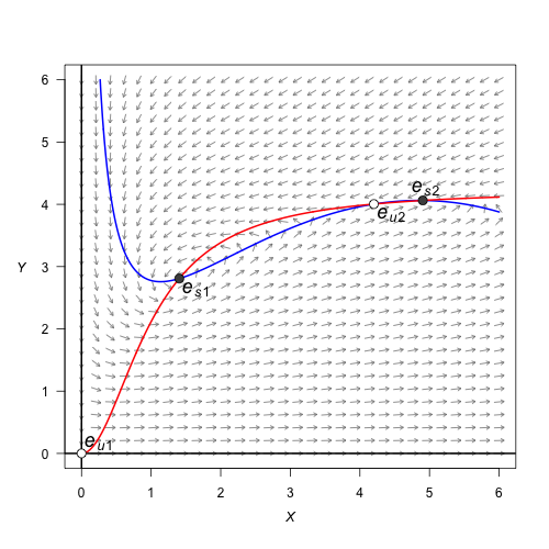
Figure 1: A stream plot of the deterministic skeleton of system (Example 1: A consumer-resource model with alternative stable states). The blue line is an $x$-nullcline (where $\frac{dx}{dt}=0$) and the red line is a $y$-nullcline (where $\frac{dy}{dt}=0$). Open circles are unstable equilibria and filled circles are stable equilibria. Made using the package phaseR.

The package phaseR (Grayling, 2014) generates a stream plot of the deterministic skeleton of the system of equations (Example 1: A consumer-resource model with alternative stable states) (Figure 1). Further, deSolve can be used to find solutions corresponding to particular initial conditions of the deterministic skeleton of system (Example 1: A consumer-resource model with alternative stable states). During the analysis of the deterministic skeleton of a system, it is important to note several things. The first is the range of $x$ and $y$ values over which relevant dynamics occur. In example 1, transitions between the stable equilibria are a primary point of interest, so one might wish to focus on a region like the one displayed in Figure 1, even though this region excludes $\mathbf{e}_{u3}$. The ranges of the variables will determine the window sizes and ranges used later in the quasi-potential calculations. Second, it is important to note if there are any limit cycles. If there are, it will be necessary to identify a point on the limit cycle. This can be accomplished by calculating a long-time solution of the system of ODEs to obtain a trajectory that settles down on the limit cycle (see example 2). Finally, it is important to note regions of phase space that correspond to unbounded solutions. As explained in subsequent sections, it is worth examining system behavior in negative phase space, even in cases where negative quantities lack physical meaning.

Step 2: Stochastic simulation

For a specified level of noise intensity, $\sigma,$ one can obtain a realization of system (Example 1: A consumer-resource model with alternative stable states). To do this, TSTraj() in QPot implements the Euler-Maruyama method. All other code/function references hereafter are found in QPot, unless specified otherwise. To generate a realization, the following arguments are required: the right-hand side of the deterministic skeleton for both equations, the initial conditions $\left(x_{0},\,y_{0}\right)$, the parameter values, the step-size $\Delta t$, and the total time length $T$.

var.eqn.x <- "(alpha*x)*(1-(x/beta)) - ((delta*(x^2)*y)/(kappa+(x^2)))"var.eqn.y <- "((gamma*(x^2)*y)/(kappa+(x^2))) - mu*(y^2)"model.state <- c(x = 1, y = 2)model.parms <- c(alpha = 1.54, beta = 10.14, delta = 1, gamma = 0.476,   kappa = 1, mu = 0.112509)model.sigma <- 0.05model.time <- 1000 # we used 12500 in the figuresmodel.deltat <- 0.025ts.ex1 <- TSTraj(y0 = model.state, time = model.time, deltat = model.deltat,     x.rhs = var.eqn.x, y.rhs = var.eqn.y, parms = model.parms, sigma = model.sigma)

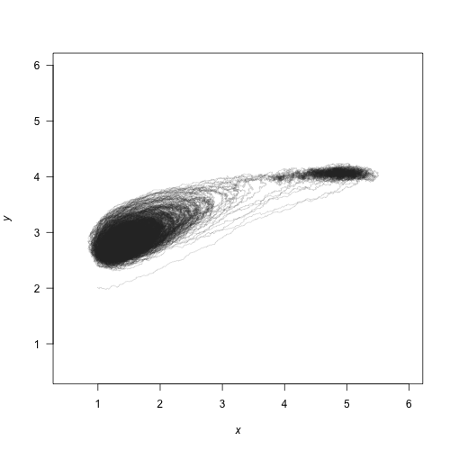
(b)

Figure 2: (a) A realization of system (Example 1: A consumer-resource model with alternative stable states) created using TSPlot(), with $x$ in blue and $y$ in red. The left side of (a) shows the time series. The right side of (a), which is enabled with the default dens = T, shows a histogram of the $x$ and $y$ values over the entire realization. (b) The realization plotted in $(x,y)$-space with dim = 2.

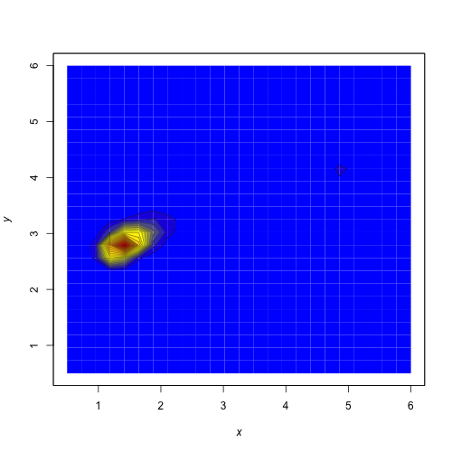
Figure 3: A density plot obtained from a realization of system (Example 1: A consumer-resource model with alternative stable states). Red corresponds to high density, and blue to low density. Plotted using the function TSDensity() with dim = 2.

Figure 2 shows a realization for $\sigma=0.05,$ $\Delta t=0.025,$ $T=1.25\times 10^{4},$ and initial condition $(x_{0},\,y_{0})=(1,\,2).$ The argument dim = 1 produces a time series plot with optional histogram side-plot. The dim = 2 produces a plot of a realization in $(x,y)$-space. If the system is ergodic, a very long realization will approximate the steady-state probability distribution. Motivated by this, a probability density function can be approximated from a long realization using the TSDensity() function (e.g., Figure 3).

TSPlot(ts.ex1, deltat = model.deltat)# Figure 2aTSPlot(ts.ex1, deltat = model.deltat, dim = 2)# Figure 2aTSDensity(ts.ex1, dim = 1)# like Figure 2a histogramTSDensity(ts.ex1, dim = 2)# Figure 3

Bounds can be placed on the state variables in all of the functions described in this subsection. For example, it might be desirable to set 0 as the minimum size of a biological population, because negative population densities are not physically meaningful. A lower bound can be imposed on the functions described in this subsection with the argument lower.bound in the function TRTraj(). Similarly, it might be desirable to set an upper bound for realizations, and hence prevent runaway trajectories (unbounded population densities are also not physically meaningful). An upper bound can be imposed on the functions described in this subsection with the argument upper.bound.

Step 3: Local quasi-potential calculation

The next step is to compute a local quasi-potential for each attractor. Because QPot deals with two-dimensional systems, “attractor" will be used synonymously with “stable equilibrium" “or stable limit cycle". A limit cycle will be considered in example 2. For now, suppose that the only attractors are stable equilibrium points, $\mathbf{e}_{si}$, $i=1,\,\ldots,\,n.$ In the example above, $n=2.$ For each stable equilibrium $\mathbf{e}_{si}$, we will compute a local quasi-potential $\Phi_{i}(x,y).$

In order to understand the local quasi-potential, it is useful consider the analogy of a particle traveling according to system (Adding stochasticity to deterministic models). In the context of example 1, the coordinates of the particle correspond to population densities, and the particle’s path corresponds to how those population densities change over time. The deterministic skeleton of (Adding stochasticity to deterministic models) can be visualized as a force field influencing the particle’s trajectory. Suppose that the particle moves along a path from a stable equilibrium $\mathbf{e}_{si}$ to a point $(x,y)$. If this path does not coincide with a solution of the deterministic skeleton, then the stochastic terms must be doing some “work” to move the particle along the path. The more work that is required, the less likely it is for the path to be a realization of system (Adding stochasticity to deterministic models). $\Phi_{i}(x,y)$ is the amount of work required to traverse the easiest path from $\mathbf{e}_{si}$ to $(x,y)$. Note that $\Phi_{i}(x,y)$ is non-negative, and it is zero at $\mathbf{e}_{si}$.

In the basin of attraction for $\mathbf{e}_{si}$, $\Phi_{i}(x,y)$ has many properties analogous to the potential function for gradient systems. Key among these properties is that the quasi-potential is non-increasing along deterministic trajectories. This means that the quasi-potential can be interpreted as a type of energy surface, and the rolling ball metaphor is still valid. The difference is that, in non-gradient systems, there is an additional component to the vector field that causes trajectories to circulate around level sets of the energy surface. This is discussed in more detail in Step 6, below.

QPot calculates quasi-potentials using an adjustment developed by Cameron (2012) to the ordered upwind algorithm (Sethian and Vladimirsky, 2001, 2003). The idea behind the algorithm is to calculate $\Phi_{i}(x,y)$ in ascending order, starting with the known point $\mathbf{e}_{si}$. The result is an expanding area where the solution is known.

Calculating $\Phi_{i}(x,y)$ with the function QPotential() requires a text string of the equations and parameter values, the stable equilibrium points, the computation domain, and the mesh size. For (Example 1: A consumer-resource model with alternative stable states), this first means inputting the equations:

$$f_{1}(x,y)=1.54x\left(1-\frac{x}{10.14}\right)-\frac{(1)x^{2}\,y}{1+x^{2}}$$

$$f_{2}(x,y)=\frac{0.476\,x^{2}\,y}{1+x^{2}}-0.112509\,y^{2}.$$

In R:

equation.x = "1.54*x*(1.0-(x/10.14))-(y*x*x)/(1.0+x*x)"equation.y = "((0.476*x*x*y)/(1+x*x))-0.112590*y*y"

The coordinates of the points $\mathbf{e}_{si}$, which were determined in Step 1, are $\mathbf{e}_{s1}=(1.4049,\,2.8081)$ and $\mathbf{e}_{s2}=(4.9040,\,4.0619)$.

eq1.x = 1.40491eq1.y = 2.80808eq2.x = 4.9040eq2.y = 4.06187

Next, the boundaries of the computational domain need to be entered. This domain will be denoted by $\left[Lx_{1},Lx_{2}\right]\times\left[Ly_{1},Ly_{2}\right]$. The ordered-upwind method terminates when the solved area encounters a boundary of this domain. Thus, it is important to choose boundaries carefully. For example, if $\mathbf{e}_{si}$ lies on one of the coordinate axes, one should not use that axis as a boundary because the algorithm will immediately terminate. Instead, one should add padding space. This is important even if the padding space corresponds to physically unrealistic values (e.g., negative population densities). For this example, a good choice of boundaries is: $Lx_{1}=Ly_{1}=-0.5,$ and $Lx_{2}=Ly_{2}=20$. This choice of domain was obtained by examining stream plots of the deterministic skeleton and density plots of stochastic realizations (Figures 1–3). The domain contains all of the deterministic skeleton equilibria, and it encompasses a large area around the regions of phase space visited by stochastic trajectories (Figures 1–3). Note that a small padding space was added to the left and bottom sides of the domain, so that the coordinate axes are not the domain boundaries.

bounds.x = c(-0.5, 20.0)bounds.y = c(-0.5, 20.0)

In some cases, it may be desirable to treat boundaries differently in the upwind algorithm. This is addressed below in the section “Boundary behavior”.

Finally, the mesh size for the discretization of the domain needs to be specified. Let $N_{x}$ be the number of grid points in the $x$-direction and $N_{y}$ be the number of grid points in the $y$-direction. Note that the horizontal distance between mesh points is $h_{x}=\frac{Lx_{2}-Lx_{1}}{N_{x}}$, and the vertical distance between mesh points is $h_{y}=\frac{Ly_{2}-Ly_{1}}{N_{y}}.$ Mesh points are considered adjacent if their Euclidean distance is less than or equal to $h=\sqrt{h_{x}^{2}+h_{y}^{2}}.$ This means that diagonal mesh points are considered adjacent. In this example, a good choice is $N_{x}=N_{y}=4100.$ This means that $h_{x}=h_{y}=0.005,$ and $h\approx 0.00707.$ In general, the best choice of mesh size will be a compromise between resolution and computational time. The mesh size must be fine enough to precisely track how information moves outward along characteristics from the initial point. Too fine of a mesh size can lead to very long computational times, though. The way that computation time scales with grid size depends on the system under consideration (see below for computation time for this example), because the algorithm ends when it reaches a boundary, which could occur before the algorithm has exhaustively searched the entire mesh area.

step.number.x = 1000 # we used 4100 in the figuresstep.number.y = 1000 # we used 4100 in the figures

The “anisotropy ratio” is another adjustable parameter for the algorithm, defined by k.x and k.y in QPotential(). For more on this, see Cameron (2012). For now, we suggest using the defaults $K_{x}=20$ and $K_{y}=20$.

The R interface implements the QPotential() algorithm using C code. By default QPotential() outputs a matrix that contains the quasi-potentials to the R session. The time required to compute the quasi-potential will depend on the size of the region and the fineness of the mesh. This example with $K_{x}=K_{y}=20$ and $N_{x}=N{y}=4100$ has approximately $1.7\times 10^{7}$ grid points, which leads to run times of approximately 2.25 min (2.5 GHz Intel Core i5 processor and 8 GB 1600 MHz DDR3 memory). When one reaches around $5\times 10^{8}$, computational time can be several hours. Setting the argument save.to.R to TRUE outputs the matrix into the R session, and setting the argument save.to.HD to TRUE saves the matrix to the hard drive as the file filename in the current working directory. For $N_{x}=N{y}=4100$, the saved file occupies 185 MB.

eq1.local <- QPotential(x.rhs = equation.x, x.start = eq1.x, x.bound = bounds.x,   x.num.steps = step.number.x, y.rhs = equation.y, y.start = eq1.y,  y.bound =   bounds.y, y.num.steps = step.number.y)

Step 3 should be repeated until local quasi-potentials $\Phi_{i}(x,y)$ have been obtained for each $\mathbf{e}_{si}$. In example 1, this means calculating $\Phi_{1}(x,y)$ corresponding to $\mathbf{e}_{s1}$ and $\Phi_{2}(x,y)$ corresponding to $\mathbf{e}_{s2}$.

eq2.local <- QPotential(x.rhs = equation.x, x.start = eq2.x, x.bound = bounds.x,   x.num.steps = step.number.x, y.rhs = equation.y, y.start = eq2.y, y.bound =   bounds.y, y.num.steps = step.number.y)

Each local quasi-potential $\Phi_{i}(x,y)$ is stored in R as a large matrix. The entries in this matrix are the values of $\Phi_{i}$ at each mesh point. To define the function on the entire domain (i.e., to allow it to be evaluated at arbitrary points in the domain, not just the discrete mesh points), bilinear interpolation is used. The values of $\Phi(x,y)$ can be extracted using the function QPInterp(). Inputs to QPInterp() include the ($x,\,y$) coordinates of interest, the ($x,\,y$) domain boundaries, and the QPotential() output (i.e., the matrix with rows corresponding to $x$-values and columns corresponding to $y$-values). QPInterp() can be used for any of the local quasi-potential or the global quasi-potential surfaces (see the next subsection).

Step 4: Global quasi-potential calculation

Recall that $\Phi_{i}(x,y)$ is the amount of “work” required to travel from $\mathbf{e}_{si}$ to $(x,y)$. This information is useful for considering dynamics in the basin of attraction of $\mathbf{e}_{si}$. In many cases, however, it is desirable to define a global quasi-potential that describes the system’s dynamics over multiple basins of attraction. If a gradient system has multiple stable states, the potential function provides an energy surface description that is globally valid. We seek an analogous global function for non-gradient systems. Achieving this requires “pasting” local quasi-potentials into a single global quasi-potential. If the system has only two attractors, one can define a global quasi-potential, though, it might be nontrivial, see example 3 ahead. In systems with three or more attractors such a task might not be possible (Freidlin and Wentzell, 2012). For a wide variety of systems, however, a relatively simple algorithm can accomplish the pasting (Graham and Tél, 1986; Roy and Nauman, 1995). In most cases, the algorithm amounts to translating the local quasi-potentials up or down so that they agree at the saddle points that separate the basins of attraction. In example 1, $\mathbf{e}_{u1}$ lies on the boundary of the basins of attraction for $\mathbf{e}_{s1}$ and $\mathbf{e}_{s2}$. Creating a global quasi-potential requires matching $\Phi_{1}$ and $\Phi_{2}$ at $\mathbf{e}_{u2}.$ $\Phi_{1}(\mathbf{e}_{u2})=0.007056$ and $\Phi_{2}(\mathbf{e}_{u2})=0.00092975.$ If one defines

$$\Phi_{2}^{*}(x,y)=\Phi_{2}(x,y)+\left(0.007056-0.00092975\right)=\Phi_{2}(x,y)+0.00612625,$$

then $\Phi_{1}$ and $\Phi_{2}^{*}$ match at $\mathbf{e}_{u2}$. Finally, define

$$\Phi(x,y)=\min(\Phi_{1}(x,y),\Phi_{2}^{*}(x,y)),$$

which is the global quasi-potential. For systems with more than two stable equilibria, this process is generalized to match local quasi-potentials at appropriate saddles. QPot automates this procedure. A fuller description of the underlying algorithm is explained in example 3, which requires a more nuanced understanding of the pasting procedure.

ex1.global <- QPGlobal(local.surfaces = list(eq1.local, eq2.local),   unstable.eq.x = c(0, 4.2008), unstable.eq.y = c(0, 4.0039), x.bound = bounds.x,   y.bound = bounds.y)

This function QPGlobal calculates the global quasi-potential by automatically pasting together the local quasi-potentials. This function requires the input of all the discretized local quasi-potentials, and the coordinates of all of the unstable equilibria. The output is a discretized version of the global quasi-potential. The length of time required for this computation will depend on the total number of mesh points; for the parameters used in example 1, it takes a couple of minutes. As with the local quasi-potentials, the values of $\Phi(x,y)$ can be extracted using the function QPInterp().

Step 5: Global quasi-potential visualization

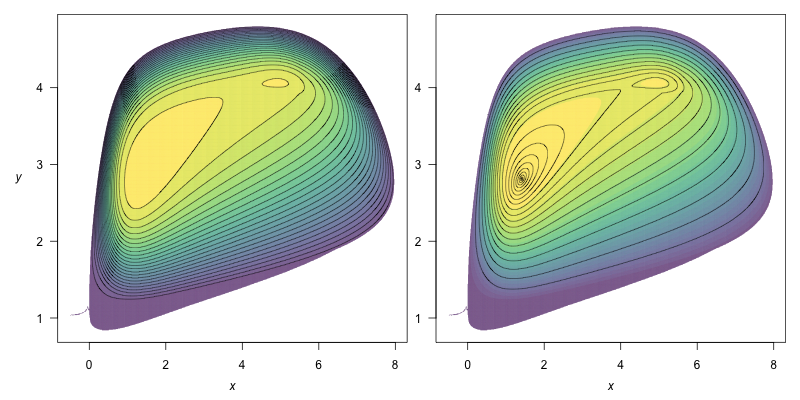
Figure 4: A contour plot of the of the quasi-potential of system (Example 1: A consumer-resource model with alternative stable states). Yellow corresponds to low values of the quasi-potential, and purple to high values. c.parm in QPContour(), can be used to condense the contour lines at the bottom of the basins for better resolution. The default creates evenly spaced contour lines (left; c.parm = 1). On the right, contour lines are condensed (c.parm = 5).

To visualize the global quasi-potential, one can simply take the global quasi-potential matrix from QPGlobal and use it to create a contour plot using QPContour() (Figure 4).

QPContour(surface = ex1.global, dens = c(1000, 1000), x.bound = bounds.x,   y.bound = bounds.y, c.parm = 5) # right side of Figure~\ref{fig:ex1qp}

QPContour() is based on the .filled.contour() function from the base package graphics. In most cases, the mesh sizes used for the quasi-potential calculation will be much finer than what is required for useful visualization. The argument dens within QPContour() reduces the points used in the graphics generation. Although it might seem wasteful to perform the original calculations at a mesh size that is finer than the final visualization, this is not so. Choosing the mesh size in the original calculations to be very fine reduces the propagation of errors in the ordered upwind algorithm, and hence leads to a more accurate numerical solution.

An additional option allows users to specify contour levels. R’s default for the contour() function creates contour lines that are equally spaced over the range of values specified by the user. In some cases, however, it is desirable to use a non-linear spacing for the contours. For example, equally-spaced contours will not capture the topography at the bottom of a basin if the changes in height are much smaller than other regions in the plot. Simply increasing the number of equally-spaced contour lines does not solve this problem, because steep areas of the plot become completely saturated with lines. QPContour() has a function for non-linear contour spacing that condenses contour lines at the bottoms of basins. Specifically, for $n$ contour lines, this function generates a list of contour levels, $\left\{v_{i}\right\}_{i=1}^{n}$, specified by:

$$v_{i}=\max(\Phi)\left(\frac{i-1}{n-1}\right)^{c}.$$

$c=1$ yields evenly-spaced contours. As $c$ increases, the contour lines become more concentrated near basin bottoms. Figure 4 shows equal contour lines (left panel) and contour lines that are concentrated at the bottom of the basin (right panel, c.parm = 5).

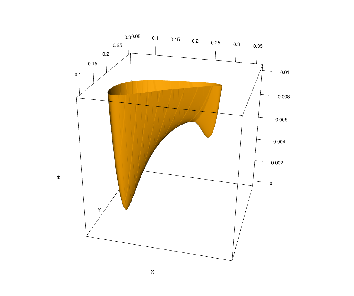
Figure 5: A 3D plot of the of the quasi-potential of system (Example 1: A consumer-resource model with alternative stable states) using persp3d() in package rgl. 3D plotting can further help users visualize the quasi-potential surfaces.

Finally, creating a 3D plot can be very useful for visualizing the features of more complex surfaces. This is especially helpful when considering the physical metaphor of a ball rolling on a surface specified by a quasi-potential (Nolting and Abbott, Accepted). R has several packages for 3D plotting, including static plotting with the base function persp() and with the package plot3D (Soetaert, 2013). Interactive plotting is provided by rgl (Adler et al., 2015). To create an interactive 3D plot for example 1 using rgl, use the code: persp3d(x = ex1.global, col = "orange"). Figure 5 shows a 3D plot of example 1 that clearly illustrates the differences between the two local basins. Users can also export the matrix of quasi-potential values and create 3D plots in other programs.

Step 6: Vector field decomposition

Recall that the deterministic skeleton (Adding stochasticity to deterministic models) can be visualized as a vector field, as shown in Figure 1. In gradient systems, this vector field is completely determined by the potential function, $V(x,y)$. The name “gradient system” refers to the fact that the vector field is the negative of the potential function’s gradient,

$$\begin{bmatrix}f_{1}(x,y)\\ f_{2}(x,y)\end{bmatrix}=-\nabla V(x,y)=-\begin{bmatrix}\frac{\partial V}{\partial x}(x,y)\\ \frac{\partial V}{\partial y}(x,y)\end{bmatrix}.$$

In non-gradient systems, the vector field can no longer be represented solely in terms of the gradient of $\Phi(x,y).$ Instead, there is a remainder component of the vector field, $\mathbf{r}(x,y)=\begin{bmatrix}r_{1}(x,y)\\ r_{2}(x,y)\end{bmatrix}.$ The vector field can be decomposed into two terms:

$$\begin{bmatrix}f_{1}(x,y)\\ f_{2}(x,y)\end{bmatrix}=-\nabla\Phi(x,y)+\mathbf{r}(x,y)=-\begin{bmatrix}\frac{\partial\Phi}{\partial x}(x,y)\\ \frac{\partial\Phi}{\partial y}(x,y)\end{bmatrix}+\begin{bmatrix}r_{1}(x,y)\\ r_{2}(x,y)\end{bmatrix}.$$

The remainder vector field is orthogonal to the gradient of the quasi-potential everywhere. That is, for every $\left(x,y\right)$ in the domain,

$$\nabla\Phi(x,y)\cdot\mathbf{r}(x,y)=0.$$

An explanation of this property can be found in Nolting and Abbott (Accepted).

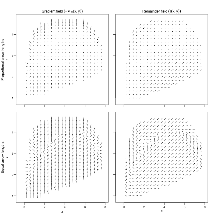
Figure 6: The gradient (left column) and remainder (right column) fields, plotted with arrow.type = "proportional" (top row) and arrow.type = "equal" (bottom row) arrow lengths using VecDecomPlot() for system (Example 1: A consumer-resource model with alternative stable states).

The remainder vector field can be interpreted as a force that causes trajectories to circulate around level sets of the quasi-potential. QPot enables users to perform this decomposition. The function VecDecomAll() calculates the vector field decomposition, and outputs three vector fields: the original deterministic skeleton, $\mathbf{f}(x,y)$; the gradient vector field, $-\nabla\Phi(x,y)$; and the remainder vector field, $\mathbf{r}(x,y)$. Each of these three vector fields can be output alone using VecDecomDS(), VecDecomGrad(), or VecDecomRem(). These vector fields can be visualized using the function VecDecomPlot(). Code to create the vector fields from VecDecomAll() is displayed below; code for generating individual vector fields can be found in help() for VecDecomDS(), VecDecomGrad(), or VecDecomRem(). The gradient and remainder vector fields are shown in the left and right columns of figure 6, respectively, with proportional vectors (top row) and equal-length vectors (bottom row). Three arguments within VecDecomPlot() are important to creating comprehensible plots: dens, tail.length, and head.length. dens specifies the number of arrows in the plot window along the $x$ and $y$ axes. The argument tail.length scales the length of arrow tails. The argument head.length scales the length of arrow heads. The function arrows() makes up the base of VecDecomPlot(), and arguments can be passed to it, as well as to plot. The code below produces all three vector fields from the multi-dimensional array returned by VecDecomAll():

# Calculate all three vector fieldsVDAll <- VecDecomAll(surface = ex1.global, x.rhs = equation.x, y.rhs =     equation.y, x.bound = bounds.x, y.bound = bounds.y)# Plot the deterministic skeleton vector fieldVecDecomPlot(field = list(VDAll[,,1], VDAll[,,2]), dens = c(25, 25),     x.bound = bounds.x, y.bound = bounds.y, x.lim = c(0, 11), y.lim = c(0, 6),     arrow.type = "equal", tail.length = 0.25, head.length = 0.025)# Plot the gradient vector fieldVecDecomPlot(field = list(VDAll[,,3], VDAll[,,4]), dens = c(25, 25),     x.bound = bounds.x, y.bound = bounds.y, arrow.type = "proportional",     tail.length = 0.25, head.length = 0.025)# Plot the remainder vector fieldVecDecomPlot(field = list(VDAll[,,5], VDAll[,,6]), dens = c(25, 25),     x.bound = bounds.x, y.bound = bounds.y, arrow.type = "proportional",     tail.length = 0.35, head.length = 0.025)

Example 2: A model with a limit cycle

Consider the following model:

$$dX=\left(-(Y-\beta)+\mu\,(X-\alpha)\left(1-(X-\alpha)^{2}-(Y-\beta)^{2}\right)\right)\,dt+\sigma\,dW_{1}$$

$$dY=\left((X-\alpha)+\mu\,(Y-\beta)\left(1-(X-\alpha)^{2}-(Y-\beta)^{2}\right)\right)\,dt+\sigma\,dW_{2}.$$ (4)

We will analyze this example with $\mu=0.2$, $\alpha=4$, and $\beta=5$.

Step 1: Analyzing the deterministic skeleton

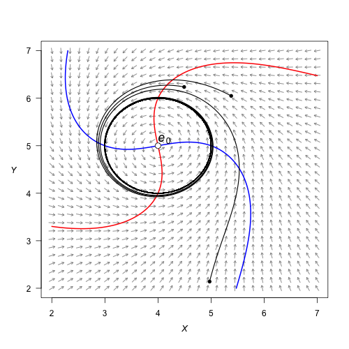
Figure 7: A stream plot of the deterministic skeleton of system (Example 2: A model with a limit cycle). The blue line is an $x$-nullcline (where $\frac{dx}{dt}=0$) and the red line is a $y$-nullcline (where $\frac{dy}{dt}=0$). The open circle is an unstable equilibrium. Particular solutions are shown as black lines, with filled circles as initial conditions. Made using the package phaseR.

The deterministic skeleton of this system has one equilibrium, $\mathbf{e}_{0}=(4,\,5),$ which is an unstable spiral point. Figure 7 shows a stream plot of the deterministic skeleton of system (Example 2: A model with a limit cycle). A particular solution of the deterministic skeleton of system (Example 2: A model with a limit cycle) can be found using rootSolve and deSolve. The stream plot and a few particular solutions suggest that there is a stable limit cycle. To calculate the limit cycle, once can find a particular solution over a long time interval (e.g., Figure 7 has three trajectories run for $T=100$). The solution will eventually converge to the limit cycle. One can drop the early part of the trajectory until only the closed loop of the limit cycle remains. There are more elegant ways to numerically find a periodic orbit (even when those orbits are unstable). For more information on these methods, see Chua and Parker (1989). In this example, the limit cycle is shown by the thick black line in Figure 7. For calculation of the quasi-potential, it is sufficient to input a single point that lies on the limit cycle. For this example, one such point is $\mathbf{z}=(4.15611,\,5.98774).$

Step 2: Stochastic simulation

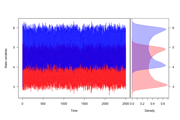
(a)

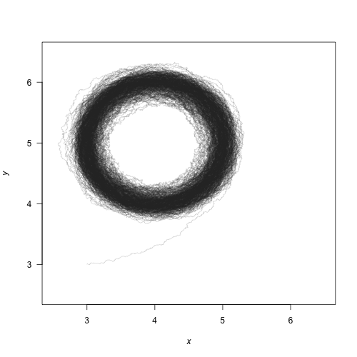
(b)

Figure 8: (a) A realization of system (Example 2: A model with a limit cycle) created using TSPlot(), with $x$ in blue and $y$ in red. The left side of (a) shows the time series. The right side of (a), which is enabled with the default dens = TRUE, shows a histogram of the $x$ and $y$ values over the entire realization. (b) The realization plotted in $(x,y)$-space (dim = 2 in the function TSPlot()).

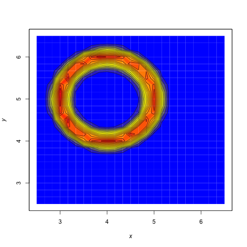
Figure 9: A density plot obtained from a realization of system (Example 2: A model with a limit cycle) using TSDensity() with dim = 2. Red corresponds to high density, and blue to low density.

Figure 8 shows a time series for a realization of (Example 2: A model with a limit cycle) with $\sigma=0.1$, $\Delta t=5\times 10^{-3}$, $T=250$ and initial condition $(x_{0},\,y_{0})=(3,\,3).$ Figure 9 shows a density plot of a realization with the same parameters, except $T=2.5\times 10^{3}.$

var.eqn.x <- "-(y-beta) + mu*(x-alpha)*(1-(x-alpha)^2-(y-beta)^2)"var.eqn.y <- "(x-alpha) + mu*(y-beta)*(1-(x-alpha)^2-(y-beta)^2)"model.state <- c(x = 3, y = 3)model.parms <- c(alpha = 4, beta = 5, mu = 0.2)model.sigma <- 0.1model.time <- 1000 # we used 2500 in the figuresmodel.deltat <- 0.005ts.ex2 <- TSTraj(y0 = model.state, time = model.time, deltat = model.deltat,     x.rhs = var.eqn.x, y.rhs = var.eqn.y, parms = model.parms, sigma = model.sigma)TSPlot(ts.ex2, deltat = model.deltat)# Figure 8aTSPlot(ts.ex2, deltat = model.deltat, dim = 2, line.alpha = 25)# Figure 8bTSDensity(ts.ex2, dim = 1)# HistogramTSDensity(ts.ex2, dim = 2)# Figure 9

Step 3: Local quasi-potential calculation

In this example, there are no stable equilibrium points. There is one stable limit cycle, and this can be used to obtain a local quasi-potential. Using $\mathbf{z}$ as the initial point for the ordered-upwind algorithm and $Lx_{1}=-0.5,$ $Ly_{1}=-0.5,$ $Lx_{2}=7.5,$ $Ly_{2}=7.5,$ $Nx=4000,$ and $Ny=4000,$ one obtains a local quasi-potential, $\Phi_{\mathbf{z}}(x,y).$ This generates the local quasi-potential $\Phi_{\mathbf{z}}(x,y)$.

eqn.x <- "-(y-5) + (0.2)*(x-4)*(1-(x-4)^2-(y-5)^2) "eqn.y <- "(x-4) + (0.2)*(y-5)*(1-(x-4)^2-(y-5)^2)"eq1.qp <- QPotential(x.rhs = eqn.x, x.start = 4.15611, x.bound = c(-0.5, 7.5),     x.num.steps = 4000, y.rhs = eqn.y, y.start = 5.98774,     y.bound = c(-0.5, 7.5), y.num.steps = 4000)

Step 4: Global quasi-potential calculation

There is only one local quasi-potential in this example, so it is the global quasi-potential, $\Phi(x,y)=\Phi_{\mathbf{z}}(x,y).$

Step 5: Global quasi-potential visualization

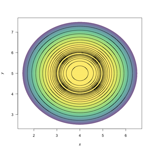
Figure 10: A contour plot of the of the quasi-potential of system (Example 2: A model with a limit cycle) using QPContour(). Yellow corresponds to low values of the quasi-potential, and purple to high values.

Figure 10 shows a contour plot of the global quasi-potential.

QPContour(eq1.qp, dens = c(1000, 1000), x.bound = c(-0.5, 7.5),y.bound = c(-0.5, 7.5), c.parm = 10)

Example 3: More complicated local quasi-potential pasting

In example 1, the procedure for pasting local quasi-potentials together into global quasi-potential was a simple, two-step process. First, one of the local quasi-potentials was translated so that the two surfaces agreed at the saddle point separating the two basins of attraction. Second, the global quasi-potential was obtained by taking the minimum of the two surfaces at each point. A general algorithm for pasting local quasi-potentials, as explained in Graham and Tél (1986) and Roy and Nauman (1995), is slightly more complicated. This process is automated in QPGlobal, but it is worth understanding the process in order to correctly interpret the outputs.

To understand the full algorithm, consider the following model:

$$dX=X\left(\left(1+\alpha_{1}\right)-X^{2}-X\,Y-Y^{2}\right)\,dt+\sigma\,dW_{1}$$

$$dY=Y\left(\left(1+\alpha_{2}\right)-X^{2}-X\,Y-Y^{2}\right)\,dt+\sigma\,dW_{2}.$$ (5)

For this analysis, let $\alpha_{1}=1.25$ and $\alpha_{2}=2.$

Step 1: Analyzing the deterministic skeleton

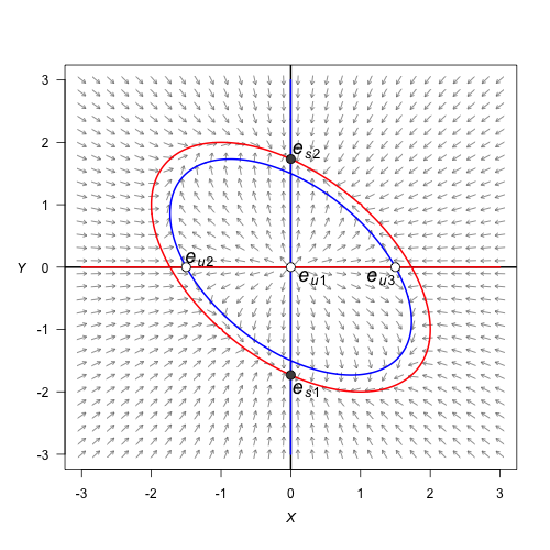
Figure 11: A stream plot of the deterministic skeleton of system (Example 3: More complicated local quasi-potential pasting). The blue line is an $x$-nullcline (where $\frac{dx}{dt}=0$) and the red line is a $y$-nullcline (where $\frac{dy}{dt}=0$). Open circles are stable equilibria and filled circles are unstable equilibria. Made using the package phaseR.

The deterministic skeleton of this system has five equilibria. These are $\mathbf{e}_{u1}=(0,0)$, $\mathbf{e}_{s1}=(0,\,-1.73205),$ $\mathbf{e}_{s2}=(0,\,1.73205),$ $\mathbf{e}_{u2}=(-1.5,\,0)$ and $\mathbf{e}_{u3}=(1.5,\,0).$ The eigenvalue analysis shows that $\mathbf{e}_{u1}$ is an unstable node, $\mathbf{e}_{s1}$ and $\mathbf{e}_{s2}$ are stable nodes, $\mathbf{e}_{u2}$ and $\mathbf{e}_{u3}$ are saddles. Figure 11 shows a stream plot of the deterministic skeleton of (Example 3: More complicated local quasi-potential pasting). The basin of attraction for $\mathbf{e}_{s1}$ is the lower half-plane, and the basin of attraction for $\mathbf{e}_{s2}$ is the upper half-plane.

Step 2: Stochastic simulation

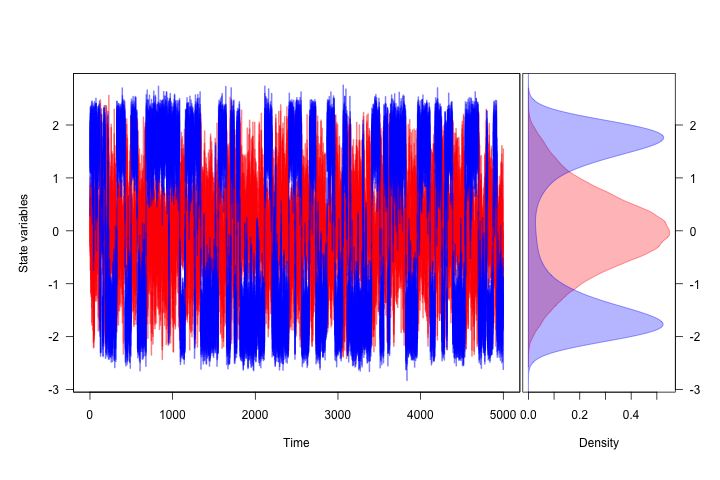
(a)

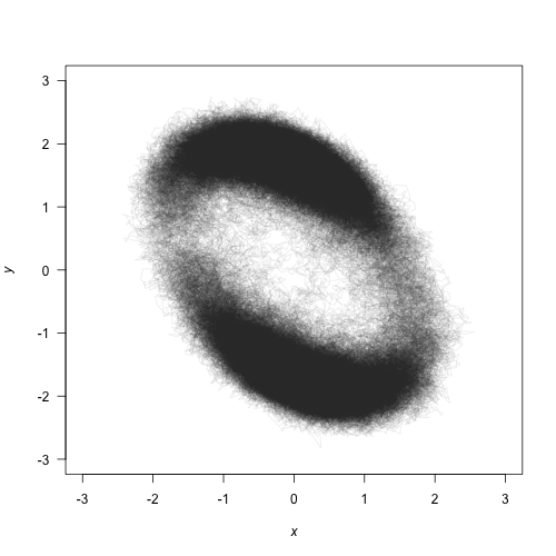
(b)

Figure 12: (a) A realization of system (Example 3: More complicated local quasi-potential pasting) created using TSPlot(), with $x$ in blue and $y$ in red. The left side in panel (a) shows the time series. The right side in panel (a), which is enabled by default with parameter dens = T in the function TSPlot(), shows a histogram of the $x$ and $y$ values over the entire realization. (b) The realization plotted in $(x,y)$-space with TSPlot() with dim = 2.

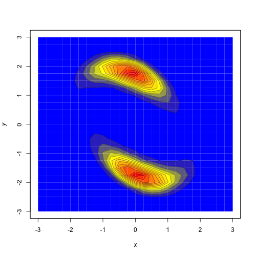
Figure 13: A density plot obtained from a realization of system (Example 3: More complicated local quasi-potential pasting) by using the function TSDensity() with dim = 2, contour.levels = 20, and contour.lwd = 0.1. Red corresponds to high density, and blue to low density.

Figure 12 shows a time series for a realization of system (Example 3: More complicated local quasi-potential pasting) with $\sigma=0.8$, $\Delta t=0.01$, $T=5000$ and initial condition $(x_{0},\,y_{0})=(0.5,\,0.5).$ Figure 13 shows a density plot of this realization.

var.eqn.x <- "x*((1+alpha1)-x*x-x*y-y*y)"var.eqn.y <- "y*((1+alpha2)-x*x-x*y-y*y)"model.state <- c(x = 0.5, y = 0.5)model.parms <- c(alpha1 = 1.25, alpha2 = 2)model.sigma <- 0.8model.time <- 5000model.deltat <- 0.01ts.ex3 <- TSTraj(y0 = model.state, time = model.time, deltat = model.deltat,     x.rhs = var.eqn.x, y.rhs = var.eqn.y, parms = model.parms, sigma = model.sigma)TSPlot(ts.ex3, deltat = model.deltat)# figure 12aTSPlot(ts.ex3, deltat = model.deltat, dim = 2 , line.alpha = 25)# figure 12bTSDensity(ts.ex3, dim = 1)# Histogram of time seriesTSDensity(ts.ex3, dim = 2 , contour.levels = 20 , contour.lwd = 0.1) # figure 13

Step 3: Local quasi-potential calculation

Two local quasi-potentials need to be calculated, $\Phi_{1}(x,y)$ corresponding to $\mathbf{e}_{s1}$, and $\Phi_{2}(x,y)$ corresponding to $\mathbf{e}_{s2}$. In both cases, sensible boundary and mesh choices are $Lx_{1}=-3,$ $Ly_{1}=-3,$ $Lx_{2}=3,$ $Ly_{2}=3,$ $Nx=6000,$ and $Ny=6000.$

equation.x = "x*((1+1.25)-x*x-x*y-y*y)"equation.y = "y*((1+2)-x*x-x*y-y*y)"bounds.x = c(-3, 3)bounds.y = c(-3, 3)step.number.x = 6000step.number.y = 6000eq1.x = 0eq1.y = -1.73205eq2.x = 0eq2.y = 1.73205eq1.local <- QPotential(x.rhs = equation.x, x.start = eq1.x, x.bound = bounds.x,     x.num.steps = step.number.x, y.rhs = equation.y, y.start = eq1.y, y.bound =     bounds.y, y.num.steps = step.number.y)eq2.local <- QPotential(x.rhs = equation.x, x.start = eq2.x, x.bound = bounds.x,     x.num.steps = step.number.x, y.rhs = equation.y, y.start = eq2.y, y.bound =     bounds.y, y.num.steps = step.number.y)

Step 4: Global quasi-potential

If one were to naively try to match the local quasi-potentials at $\mathbf{e}_{u2}$, then they would not match at $\mathbf{e}_{u3}$, and vice versa. To overcome this problem, it is necessary to think more carefully about how trajectories transition between basins of attraction. This issue can be dealt with rigorously (Graham and Tél, 1986; Roy and Nauman, 1995), but the general principles are outlined here. Let $\Omega_{1}$ be the basin of attraction corresponding to $\mathbf{e}_{s1}$ and $\Omega_{2}$ be the basin of attraction corresponding to $\mathbf{e}_{s2}$. Let $\partial\Omega$ be the separatrix between these two basins (i.e., the $x$-axis). The most probable way for a trajectory to transition from $\Omega_{1}$ to $\Omega_{2}$ involves passing through the lowest point on the surface specified by $\Phi_{1}$ along $\partial\Omega$. Examination of $\Phi_{1}$ indicates that this point is $\mathbf{e}_{u2}$. In the small-noise limit, the transition rate from $\Omega_{1}$ to $\Omega_{2}$ will correspond to $\Phi_{1}\left(\mathbf{e}_{u2}\right)$. Similarly, the transition rate from $\Omega_{2}$ to $\Omega_{1}$ will correspond to $\Phi_{2}\left(\mathbf{e}_{u3}\right)$. The transition rate into $\Omega_{1}$ must equal the transition rate out of $\Omega_{2}$. Therefore, the two local quasi-potentials should be translated so that the minimum heights along the separatrix are the same. In other words, one must define translated local quasi-potentials $\Phi^{*}_{1}(x,y)=\Phi_{1}(x,y)+c_{1}$ and $\Phi^{*}_{2}(x,y)=\Phi_{2}(x,y)+c_{2}$ so that

$$\min{\left(\Phi^{*}_{1}(x,y)|(x,y)\in\partial\Omega\right)}=\min{\left(\Phi^{*}_{2}(x,y)|(x,y)\in\partial\Omega\right)}.$$

In example 1, the minima of both local quasi-potentials occurred at the same point, so the algorithm amounted to matching at that point. In example 3, the minimum saddle for $\Phi_{1}$ is $\mathbf{e}_{u2}$ and the minimum saddle for $\Phi_{2}$ is $\mathbf{e}_{u3}$; the heights of the surfaces at these respective points should be matched. Thus, $c_{1}=\Phi_{2}(e_{u3})-\Phi_{1}(e_{u3})$ and $c_{2}=\Phi_{1}(e_{u2})-\Phi_{2}(e_{u2})$. Conveniently in example 3, this is satisfied without requiring any translation (one can use $c_{1}=c_{2}=0$). Finally, the global quasi-potential is found by taking the minimum value of the matched local quasi-potentials at each point. This process is automated in QPot, but users can also manipulate the local quasi-potential matrices manually to verify the results. This is recommended when dealing with unusual or complicated separatrices. The code below applies the automated global quasi-potential calculation to example 3.

ex3.global <- QPGlobal(local.surfaces = list(eq1.local, eq2.local),unstable.eq.x     = c(0, -1.5, 1.5), unstable.eq.y = c(0, 0, 0), x.bound = bounds.x, y.bound =     bounds.y)

Step 5: Global quasi-potential visualization

Figure 14 shows a contour plot of the global quasi-potential. Note that the surface is continuous, but not smooth. The lack of smoothness is a generic feature of global quasi-potentials created from pasting local quasi-potentials. Cusps usually form when switching from the part of solution obtained from one local quasi-potential to the other.

QPContour(ex3.global, dens = c(1000, 1000), x.bound = bounds.x, y.bound =     bounds.y, c.parm = 5)

Boundary behavior

It is important to consider the type of behavior that should be enforced at the boundaries and on coordinate axes ($x=0$ and $y=0$). By default, the ordered-upwind method computes the quasi-potential for the system defined by the user, without regard for the influence of the boundaries or the significance of these axes. In some cases, however, a model is only valid in a subregion of phase space. For example, in many population models, only the non-negative phase space is physically meaningful. In such cases, it is undesirable to allow the ordered-upwind method to consider trajectories that pass through negative phase space. In the default mode for QPotential(), if $(x,y)$ lies in positive phase space, $\Phi(x,y)$ can be impacted by the vector field in negative phase space, if the path corresponding to the minimum “work” passes through negative phase space. The argument bounce = ’d’ corresponds to this (d)efault behavior. A user can prevent the ordered upwind method from passing trajectories through negative phase space by using the option bounce = ’p’ for (p)ositive values only. This option can be interpreted as a reflecting boundary condition. It forces the front of solutions obtained by the ordered upwind method to stay in the defined boundaries, in this case the positive phase space. A more generic option is bounce = ’b’ for (b)ounce, which reflects based on the user-supplied boundaries. Even using this option, it is still wise to have padding space along coordinate boundaries to prevent premature termination of the algorithm, which is set with bounce.edge.

Different noise terms

In the cases considered so far, the noise terms for the $X$ and $Y$ variables have had identical intensity. This was useful for purposes of illustration in the algorithm, but it will often be untrue of real-world systems. Fortunately, QPot can accomodate other noise terms with coordinate transforms. Consider a system of the form:

$$dX=f_{1}(X,Y)\,dt+\sigma\,g_{1}\,dW_{1}$$

$$dY=f_{2}(X,Y)\,dt+\sigma\,g_{2}\,dW_{2}.$$ (6)

$\sigma$ is a scaling parameter that specifies the overall noise intensity. The parameters $g_{1}$ and $g_{2}$ specify the relative intensity of the two noise terms. To transform this system into a form that is useable for QPot, make the change of variable $\tilde{X}=g_{1}^{-1}X$ and $\tilde{Y}=g_{2}^{-1}Y.$ In the new coordinates, the drift terms (that is, the terms multiplied by $dt$), will be different. These new drift terms can be incorporated into the deterministic skeleton that is input into QPot. After obtaining the global quasi-potential for these transformed coordinates, one can switch back to the original coordinates for plotting.

Many models contain multiplicative noise terms. These are of the form:

$$dX=f_{1}(X,Y)\,dt+\sigma\,g_{1}\,X\,dW_{1}$$

$$dY=f_{2}(X,Y)\,dt+\sigma\,g_{2}\,Y\,dW_{2}.$$ (7)

To transform this system into a form that is useable for QPot, make the change of variable $\tilde{X}=g_{1}^{-1}\ln\left(X\right)$ and $\tilde{Y}=g_{1}^{-1}\ln\left(Y\right).$ This coordinate change is non-linear, so Itô’s lemma introduces extra terms into the drift of the transformed equations. If $\sigma$ is small, though, these terms can be discounted, and the new drift terms will remain independent of $\sigma.$ These new drift terms can be input into QPot. After obtaining the global quasi-potential for these transformed coordinates, one can switch back to the original coordinates.

Conclusion

QPot is an R package that provides several important tools for analyzing two-dimensional systems of stochastic differential equations. These include functions for generating realizations of the stochastic differential equations, and for analyzing and visualizing the results. A central component of QPot is the calculation of quasi-potential functions, which are highly useful for studying stochastic dynamics. For example, quasi-potential functions can be used to compare the stability of different attractors in stochastic systems, a task that traditional linear stability analysis is poorly suited for (Nolting and Abbott, Accepted). By offering an intuitive way to quantify attractor stability, quasi-potentials are poised to become an important means of understanding phenomena like metastability and alternative stable states. QPot makes quasi-potentials accessible to R users interested in applying this new framework.

Author contributions

K.C.A, C.M.M., B.C.N., and C.R.S. designed the project. M.K.C. wrote the C code for finding the quasi-potential; C.M.M. and C.R.S. wrote the R code and adapted the C code.

Christopher M. Moore
Department of Biology
Case Western Reserve University
United States
life.dispersing@gmail.com

Christopher R. Stieha
Department of Biology
Case Western Reserve University
United States
stieha@hotmail.com

Ben C. Nolting
Department of Biology
Case Western Reserve University
United States
ben.nolting@case.edu

Maria K. Cameron
Department of Mathematics
University of Maryland
United States
cameron@math.umd.edu

Karen C. Abbott
Department of Biology
Case Western Reserve University
United States
kcabbott@case.edu

Figures

(a)

Figure 14: A contour plot of the quasi-potential of system (Example 3: More complicated local quasi-potential pasting) using the function QPContour(). Yellow corresponds to low values of the quasi-potential, and purple to high values.

References

- Adler et al. (2015) D. Adler, D. Murdoch, O. Nenadic, S. Urbanek, M. Chen, A. Gebhardt, B. Bolker, G. Csardi, A. Strzelecki, and A. Senger. rgl: 3d visualization device system for R using OpenGL, 2015. URL https://cran.r-project.org/package=rgl.
- Allen (2007) E. J. Allen. Modeling with Ito stochastic differetnial equations, volume 22 of Mathematical modelling: theory and applications. Springer, 2007.
- Cameron (2012) M. K. Cameron. Finding the quasipotential for nongradient SDEs. Physica D, 241(18):1532–1550, 2012.
- Chua and Parker (1989) T. S. P. L. Chua and T. S. Parker. Practical umerical algorithms for chaotic systems, chapter 5. Springer-Verlag, 1989.
- Collie and Spencer (1994) J. S. Collie and P. D. Spencer. Modeling predator-prey dynamics in a fluctuating environment. Canadian Journal of Fisheries and Aquatic Sciences, 51(12):2665–2672, 1994.
- Freidlin and Wentzell (2012) M. I. Freidlin and A. D. Wentzell. Random perturbations of dynamical systems, volume 260. Springer, 2012.
- Graham and Tél (1986) R. Graham and T. Tél. Nonequilibrium potential for coexisting attractors. Physical Review. A., 33(2):1322–1337, 1986.
- Grayling (2014) M. J. Grayling. phaseR: An R package for phase plane analysis of autonomous ode systems. The R Journal, pages 43–51, 2014.
- Iacus (2009) S. M. Iacus. Simulation and inference for stochastic differential equations: with R examples, volume 1. Springer Science & Business Media, 2009.
- Nolting and Abbott (Accepted) B. C. Nolting and K. C. Abbott. Balls, cups, and quasi-potentials: quantifying stability in stochastic systems. Ecology, Accepted.
- Roy and Nauman (1995) R. V. Roy and E. Nauman. Noise-induced effects on a non-linear oscillator. Journal of Sound and Vibration, 1995.
- Sethian and Vladimirsky (2001) J. A. Sethian and A. Vladimirsky. Ordered upwind methods for static Hamilton-Jacobi equations. Proceedings of the National Academy of Sciences, 98(20):11069–11074, 2001. doi: 10.1073/pnas.201222998.
- Sethian and Vladimirsky (2003) J. A. Sethian and A. Vladimirsky. Ordered upwind methods for static Hamilton-Jacobi equations: Theory and algorithms. SIAM Journal on Numerical Analysis, 41(1):325–363, 2003. doi: 10.1137/S0036142901392742.
- Soetaert (2013) K. Soetaert. plot3d: Plotting multi-dimentional data in R, 2013. URL https://cran.r-project.org/package=plot3D.
- Soetaert and Herman (2008) K. Soetaert and P. M. Herman. A practical guide to ecological modelling: using R as a simulation platform. Springer Science & Business Media, 2008.
- Soetaert et al. (2010) K. Soetaert, T. Petzoldt, and R. W. Setzer. Solving differential equations in R: Package deSolve. Journal of Statistical Software, 33(9):1–25, 2010.
- Steele and Henderson (1981) J. Steele and E. Henderson. A simple plankton model. American Naturalist, pages 676–691, 1981.