Measurement and modeling of polarized specular neutron reflectivity in large magnetic fields

Abstract

The presence of a large applied magnetic field removes the degeneracy of the vacuum energy states for spin-up and spin-down neutrons. For polarized neutron reflectometry, this must be included in the reference potential energy of the Schrödinger equation that is used to calculate the expected scattering from a magnetic layered structure. For samples with magnetization that is purely parallel or antiparallel to the applied field which defines the quantization axis, there is no mixing of the spin states (no spin-flip scattering) and so this additional potential is constant throughout the scattering region. When there is non-collinear magnetization in the sample however, there will be significant scattering from one spin state into the other and the reference potentials will differ between the incoming and outgoing wavefunctions, changing the angle and intensities of the scattering. The theory of the scattering and recommended experimental practices for this type of measurement are presented, as well as an example measurement.

Procedure for polarized neutron reflectometry when the Zeeman corrections are significant, which occurs when both the magnetic anisotropy and applied magnetic field are significant. Calculations and recommended procedure in an example system are provided.

1 Introduction

Polarized specular neutron reflectometry measurements require at least a small magnetic field to be applied throughout the measurement apparatus, in order to maintain a well-defined neutron quantization axis. In addition, a larger field is often applied at the sample position in order to manipulate the magnetic state of the sample [PNRMajkrzakChapter]. The difference in the Zeeman energy for a spin-up vs. a spin-down neutron can lead to observable shifts in both the angle and intensity of scattering for even modest applied fields (10s of mT) when spin-flip scattering is appreciable; when the spin-flip cross-section is small compared to the non-spin-flip, the corrections remain small.

This so-called Zeeman shift in the spin-flipped reflected neutrons was first described by Felcher et al. [felcher1995zeeman], and observed by many others [felcher1996observation]; in Ref. [kozhevnikov2012data] a clear description of the geometry of the incident and scattered beams is presented. The reflectivity calculation formalism including the Zeeman term is briefly described in [vandeKruijs2000189, PhysRevB.83.174418], but to our knowledge a detailed description of the calculation is not available in the literature, nor has such a calculation been incorporated into commonly-used modeling software.

These shifts are not a major concern in many experiments [PhysRevB.83.174418] because the effect is significant only when there is both a large applied field and strong spin-flip scattering. At low fields the corrections are minimal, and at high fields the magnetization tends to align parallel to the applied field, so there is insignificant spin-flip scattering. However, there are important cases where accounting for the Zeeman shift is necessary for appropriately measuring and analyzing data. A technologically relevant example is the study of high anisotropy magnetic material used in advanced data storage applications [PhysRevB.83.174418]. In such cases the sample magnetization can be non-collinear with even large applied fields.

In this paper we will address the requirements for setting up a measurement in a large field in the case where the spin-flip scattering is not negligible; we present the changes that need to be made to a commonly-used existing computer algorithm (implemented in gepore.f [PNRMajkrzakChapter]) in order to correctly calculate the scattering, and we present recommended practices for performing the measurements when the applied magnetic field $\vec{H}$ and magnetization $\vec{M}$ are both large, and not parallel to each other. This implies a large magnetic anisotropy in the system. We take advantage of the large shape anisotropy in a thin film of a soft magnetic material in the example experiment section of this paper to clearly show the effects we are discussing.

We must also address the meaning of the word “specular”; in many texts on reflectivity the definition is given that the angle of incidence equals the angle of reflection, or that the out-of-plane component of the momentum of the incoming beam $k_{z,\mathrm{in}}$ is equal in magnitude to that of the outgoing reflected beam $k_{z,\mathrm{out}}$. Here we will use a more functional definition based on the momentum transfer $\vec{Q}\equiv\vec{k}_{\mathrm{in}}-\vec{k}_{\mathrm{out}}$; we define the reflectivity as specular on the condition that the in-plane momentum transfers $Q_{x}=0$ and $Q_{y}=0$, so that the momentum transfer $\vec{Q}\equiv Q_{z}\hat{z}$ (perpendicular to the surface) as is expected when reflecting from planar layered samples.

As we will demonstrate, some of the kinetic energy along $\hat{z}$ is traded for potential energy during a spin-flip process, so the earlier definitions do not apply in this circumstance, while $\vec{Q}$ remains strictly out-of-plane.

2 Boundary conditions

Starting with the general Schrödinger equation for a neutron with spin $\frac{1}{2}$:

$$\left[-\frac{\hbar^{2}}{2m}\nabla^{2}\hat{1}+\hat{V}(\mathbf{r})-E\hat{1}\right]\begin{pmatrix}\psi^{+}(\mathbf{r})\\ \psi^{-}(\mathbf{r})\end{pmatrix}=0$$ (1)

where $\psi^{\pm}$ is the spin-dependent wavefunction for the neutron, $\hat{1}=\begin{pmatrix}1&0\\ 0&1\end{pmatrix}$, $\nabla^{2}$ is the Laplacian (spatial second derivative) and the hatted components indicate a Pauli spin matrix with $z^{\prime}$ as the quantization axis. We use the notation $z^{\prime}$ for coordinates in the spin quantization reference frame to distinguish it from the scattering geometrical reference frame where $z$ is defined to be the surface normal direction for the planar sample, and there is no requirement that $\hat{z}\parallel\hat{z}^{\prime}$. The potential of the particle is made up of a scalar nuclear potential $V_{\mathrm{nuc}}$ and a magnetic potential due to the field $\mathrm{B}$:

$$\hat{V}=\mu_{N}\boldsymbol{\sigma}\cdot\mathbf{B}+V_{\mathrm{nuc}}\hat{1}$$ (2)

where

$$\boldsymbol{\sigma}\cdot\mathbf{B}=\begin{pmatrix}0&1\\ 1&0\end{pmatrix}B_{x^{\prime}}+\begin{pmatrix}0&-i\\ i&\phantom{-}0\end{pmatrix}B_{y^{\prime}}+\begin{pmatrix}1&\phantom{-}0\\ 0&-1\end{pmatrix}B_{z^{\prime}}$$ (3)

In the “prepared” spin-polarized beam, we define the direction of the guide field to be $\hat{z}^{\prime}$, so there are no off-diagonal elements to the potential above (because $B_{x^{\prime}}\equiv B_{y^{\prime}}\equiv 0$) and the equation decouples into two linear equations for potentials with $V=V_{\mathrm{nuc}}\pm\mu_{N}B_{z^{\prime}}$.

When the beam enters the fronting medium with non-negligible $B$, there is no physical restriction on the direction of $\vec{B}$, but from an experimental design perspective we note that if the magnetic field in the fronting medium is not parallel to the applied laboratory field direction $(\hat{z}^{\prime})$, i.e. there is a non-zero $B_{x^{\prime}}$ or $B_{y^{\prime}}$ component to the field in this region, the wavefunction will be angularly split due to the field-dependent difference between $k_{F,x}^{+}$ and $k_{F,x}^{-}$. The mutual coherence of the two resulting beams will be impractical to calculate over the macroscopic distances the beam will then travel after being split.

This is not to be confused with the angular splitting which occurs as the the beam interacts with the horizontal layers of the sample, which is what is usually being discussed when describing reflectivity, and which is fully taken into account in the calculations below.

Now restricting ourselves to the case in which the $B$-field in the fronting medium is parallel to the guide field outside the fronting medium, we can fully describe the interaction of the neutron with the sample as in Fig. 1.

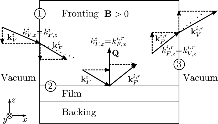
Figure 1: neutron entering field and nuclear potential region from the side.

The incident neutron is “prepared” in either the $I^{+}$ or $I^{-}$ spin state with techniques described elsewhere [dura2006and, PNRMajkrzakChapter] and neglecting the contribution of a very small magnetic guide field, the total energy of both states is nearly the same for the same $\mathbf{k}_{V}$, and is equal to the kinetic energy:

$$E^{+}_{V,xyz}\approx E^{-}_{V,xyz}\approx\frac{\hbar^{2}}{2m}\left(k_{V,x}^{2}+k_{V,y}^{2}+k_{V,z}^{2}\right)$$ (4)

We note that the problem as defined has no $y$-dependence; there are no interfaces along that direction (out of the page of the figure) and so the solution for the wave equation along $y$ is for a plane wave $e^{ik_{y}y}$ with constant kinetic energy that can be included in the total energy $E$ and the problem treated as a 2-dimensional Schrodinger equation in $x$ and $z$, with

$$\begin{array}[]{l l}E_{V,xz}^{\pm}&\approx\frac{\hbar^{2}}{2m}\left(k_{V,x}^{2}+k_{V,z}^{2}\right)\\[3.00003pt] {}&=E_{V,xyz}^{\pm}-\frac{\hbar^{2}}{2m}k_{V,y}^{2}\end{array}$$ (5)

When the neutron enters the fronting medium at boundary \raisebox{-.9pt} {1}⃝ as shown in Fig. 1, the potential energy changes in a spin-dependent way, so that

$$E^{+}_{F,xz}=\frac{\hbar^{2}}{2m}\left[(k_{F,x}^{+})^{2}+(k_{F,z}^{+})^{2}+4\pi(\rho_{F,N}+\rho_{F,B})\right]$$ (6)

$$E^{-}_{F,xz}=\frac{\hbar^{2}}{2m}\left[(k_{F,x}^{-})^{2}+(k_{F,z}^{-})^{2}+4\pi(\rho_{F,N}-\rho_{F,B})\right]$$ (7)

where the notation $\mathbf{k}_{F}^{i}$ indicates the wavevector in the medium ($F$ for fronting and $V$ for vacuum) with spin state $i$ ($+$ or $-$). The nuclear scattering length density of the fronting medium $\rho_{F,N}$ depends on the isotopic composition of the medium, while $\rho_{F,B}$ is the magnetic scattering length density, which can be calculated from the magnetic field in that layer by

$$\rho_{B}=\frac{2\mu_{n}m_{n}|\vec{B}|}{4\pi\hbar^{2}}\approx B\times 2.31605\times 10^{-6}\textrm{\AA}^{-2}\textrm{T}^{-1}$$ (8)

where $\mu_{n},m_{n}$ are the magnetic moment and mass of the neutron, respectively and $B$ is the magnetic field in the fronting medium (in Teslas).

Since the magnetic field inside the vertical boundary is parallel to (though possibly much bigger than) the field outside, the $(+)$ or $(-)$ spin state inside the vertical boundary matches the prepared state. Also, by symmetry $k_{z}$ must be preserved across the vertical boundary \raisebox{-.9pt} {1}⃝, between the vacuum and the fronting medium, so $k_{V,z}=k_{F,z}$. Since $E_{V,xz}^{+}=E_{F,xz}^{+}$ as well, this means that

$$(k_{F,x}^{+})^{2}=(k_{V,x})^{2}-4\pi(\rho_{F,N}+\rho_{F,B})$$ (9)

$$(k_{F,x}^{-})^{2}=(k_{V,x})^{2}-4\pi(\rho_{F,N}-\rho_{F,B})$$

which changes the angle of the neutron beam inside the fronting medium (this is refraction, as indicated by the shortened $k_{x}$ on the right side of boundary \raisebox{-.9pt} {1}⃝ in Fig. 1). The energy trade in $k_{x}$ is reversed when the neutron exits the fronting at boundary \raisebox{-.9pt} {3}⃝; the $k_{V,x}$ on the right is the same as it is on the left. This is not in general true for $k_{V,z}$, as we will see.

Now we consider the next set of boundaries in the problem: the horizontal interfaces of the sample under investigation; the first of these is the top interface \raisebox{-.9pt} {2}⃝ between the fronting and the sample. When the neutron interacts with this structure, it is possible to have a spin-flip event, so we introduce a second indicator $r$ (for reflected) in the notation $\mathbf{k}_{F}^{i,r}$ for the spin state of the outgoing neutron (still in the fronting medium). We retain the indicator $i$ for the incident neutron spin state because this determines the energy in the fronting, as described above.

We are considering the standard specular reflectometry case where the sample under investigation is homogenous in-plane; so while $k_{z}$ was conserved across boundary \raisebox{-.9pt} {1}⃝, now $k_{x}$ is conserved across the boundaries like \raisebox{-.9pt} {2}⃝, so

$$k_{F,x}^{+,-}=k_{F,x}^{+,+}=k_{F,x}^{+}$$ (10)

$$k_{F,x}^{-,+}=k_{F,x}^{-,-}=k_{F,x}^{-}$$

and because the total energy of the neutron is conserved during elastic scattering, we can write

$$\begin{array}[]{l l}E_{F,xz}^{+,-}&=\frac{\hbar^{2}}{2m}\left[(k_{F,x}^{+,-})^{2}+(k_{F,z}^{+,-})^{2}+4\pi(\rho_{F,N}-\rho_{F,B})\right]\\[3.00003pt] {}&=E_{F,xz}^{+}\end{array}$$ (11)

Subtracting this from Eq. 6 gives

$$(k_{F,z}^{+,-})^{2}=(k_{F,z}^{+})^{2}+8\pi\rho_{F,B}$$ (12)

In a similar fashion for the $(-)$ state, we can obtain

$$(k_{F,z}^{-,+})^{2}=(k_{F,z}^{-})^{2}-8\pi\rho_{F,B}$$ (13)

While the non-spin-flipped neutrons are not shifted:

$$(k_{F,z}^{+,+})^{2}=(k_{F,z}^{+})^{2}$$ (14)

$$(k_{F,z}^{-,-})^{2}=(k_{F,z}^{-})^{2}$$

At the next boundary \raisebox{-.9pt} {3}⃝ where the neutrons exit the fronting material and go back into the laboratory environment (vacuum) $k_{z}$ is again conserved by symmetry, as it was at \raisebox{-.9pt} {1}⃝, so the shift in the spin-flipped $k_{z}$ is carried across this boundary ($k_{V,z}^{i,r}=k_{F,z}^{i,r}$ for all $i,r$.)

The difference between $k_{V,z}^{+,-}$ and $k_{V,z}^{+,+}$ leads to a different propagation direction for the spin-flipped neutron; this measurable angular shift is referred to as the Zeeman splitting.

There are values of $k_{F,z}^{-}$ for which $(k_{F,z}^{-})^{2}<8\pi\rho_{F,B}$ and therefore the calculated momentum squared for the spin-flipped reflection $(k_{F,z}^{-,+})^{2}$ is negative, so that $k_{F,z}^{-,+}$ becomes purely imaginary. The calculated amplitude for this reflection is valid at the interface, but this is an evanescent wave that decays as it moves away from the sample. The value of the measured reflectivity corresponds to the amplitude at the detector, and thus is effectively zero in this case.

2.1 Details of magnetic field geometry

In the above discussion, the transition from vacuum with zero applied field to a high-field region (also with a possibly non-zero nuclear scattering length density) was described as a sharp boundary perpendicular to the sample plane (along $x$). In that case, the momentum along $z$ is unchanged by the transition: $k_{F,z}=k_{V,z}$, and energy conservation leads only to a change in $k_{x}$: $(k_{F,x}^{+})^{2}+4\pi(\rho_{F,N}+\rho_{F,B})=k_{V,x}^{2}$.

In real laboratory environments the magnetic field transition is not as abrupt as what is shown in Fig. 1, and the direction is not perfectly defined, though typically the applied magnetic field is realized in a small volume centered on the sample and the field gradient experienced by the probe neutron is to first order radial with respect to the sample. Since for any gradient potential the momentum components perpendicular to the gradient direction are conserved throughout the interaction with the potential, the abruptness of the transition is irrelevant and only the direction is important.

So, compared to a more realistic radial magnetic potential gradient parallel to the neutron momentum we expect that by using our simplified rectangular boundary conditions (where the sharp gradient at that boundary is along $\hat{x}$ and is nearly but not quite parallel to $\vec{k}_{\mathrm{(in)}}$) we introduce an error in the calculated $(k_{F,z}^{\pm})^{2}$ proportional to $\sin^{2}\delta$, where $\delta$ is the angle between the normal to the rectangular boundary and $\vec{k}_{\mathrm{(in)}}$. Because of the right angle between that boundary and the film surface, it ends up that $\delta$ coincides with the incident angle $\theta_{\mathrm{in}}$ of the neutron on the film surface.

At the small angles ($\theta_{\mathrm{in}}<$ 6 deg.) commonly seen for the incident angle during a reflectometry measurement, this results in a maximum correction to $(k_{F,z}^{\pm})^{2}$ from the model proposed above, on the order of 1 percent of $\pm 4\pi\rho_{B}$ (with the opposite correction made to $E_{F,z}^{\pm}$.) At the even smaller angles ($\theta_{\mathrm{in}}\approx$ 0.5 deg.) near the critical edge where these shifts might affect the modeling, the correction is just 0.01 percent of the magnetic scattering length density. For this reason in many cases it is a reasonable approximation that all the of the kinetic energy shift in the Fronting region prior to the sample is along the $x$-direction, as defined by the sample coordinate system in Fig. 1.

3 Calculation of the spin-dependent reflectivity

3.1 1d Schrödinger equation

Again considering the region between \raisebox{-.9pt} {1}⃝ and \raisebox{-.9pt} {3}⃝ as above, we can calculate the reflectivity of the horizontally-layered structure there by reducing the Schrödinger equation to a single spatial dimension $z$ and solving with the boundary conditions laid out above. Since the potential is constant as a function of $x$ in this region (as it is for $y$ everywhere,) and $V(\mathbf{r})=V(z)$, the one-dimensional plus spin Schrödinger equation for the neutron is then [PNRMajkrzakChapter],

$$\left[-\frac{\hbar^{2}}{2m}\frac{\partial^{2}}{\partial z^{2}}\hat{1}+\hat{V}(z)-E_{F,z}^{i}\hat{1}\right]\begin{pmatrix}\psi^{i,+}(z)\\ \psi^{i,-}(z)\end{pmatrix}=0$$ (15)

where

$$\begin{array}[]{l l}\hat{V}(z)\!\!&=\begin{pmatrix}V^{++}(z)&V^{+-}(z)\\ V^{-+}(z)&V^{--}(z)\end{pmatrix}\\[11.99998pt] {}&=\displaystyle\frac{4\pi\hbar^{2}}{2m}\!\!\begin{pmatrix}\rho_{N}+\rho_{Bz^{\prime}}&\rho_{Bx^{\prime}}-i\rho_{By^{\prime}}\\ \rho_{Bx^{\prime}}+i\rho_{By^{\prime}}&\rho_{N}-\rho_{Bz^{\prime}}\end{pmatrix}(z)\end{array}$$ (16)

and we fold the constant kinetic energy along $x$ into $E$ as we did for $y$ before:

$$E^{i}_{F,z}=E^{i}_{F,xz}-\frac{\hbar^{2}}{2m}k_{F,x}^{2}$$ (17)

$E_{F,z}^{i}$ depends on the spin state of the incident neutron as well as the potential in the fronting medium, as

$$E_{F,z}^{\pm}=\frac{\hbar^{2}}{2m}\left[4\pi(\rho_{F,N}\pm\rho_{F,B})+(k_{V,z})^{2}\right]$$ (18)

A set of solutions to Eq. 15 is laid out in [PNRMajkrzakChapter], as (except now keeping track of the polarization $i$ of the incident state)

$$\psi^{i,+}(z)=\sum_{j=1}^{4}C^{i}_{j}e^{S^{i}_{j}z}$$ (19)

$$\psi^{i,-}(z)=\sum_{j=1}^{4}\mu_{j}C^{i}_{j}e^{S^{i}_{j}z}$$

where

$$S_{1}^{i} = \sqrt{4\pi(\rho_{N}+\rho_{B})-\frac{2m}{\hbar^{2}}E_{F,z}^{i}}$$ (20)

$$S_{2}^{i} = -S_{1}^{i}$$

$$S_{3}^{i} = \sqrt{4\pi(\rho_{N}-\rho_{B})-\frac{2m}{\hbar^{2}}E_{F,z}^{i}}$$

$$S_{4}^{i} = -S_{3}^{i}$$

$$\begin{array}[]{l}\displaystyle\mu_{1}=\mu_{2}=\frac{B+B_{x^{\prime}}+iB_{y^{\prime}}-B_{z^{\prime}}}{B+B_{x^{\prime}}-iB_{y^{\prime}}+B_{z^{\prime}}}\\[11.99998pt] \displaystyle\mu_{3}=\mu_{4}=\frac{-B+B_{x^{\prime}}+iB_{y^{\prime}}-B_{z^{\prime}}}{-B+B_{x^{\prime}}-iB_{y^{\prime}}+B_{z^{\prime}}}\end{array}$$ (21)

and the $C_{j}^{i}$ are the complex coefficients of the 4 components.

Within the fronting medium $F$ the propagation constants $S$ are equal to simply the incident wave value $ik_{F,z}$, since the potentials $\rho$ cancel between Eqs. 18 and 20 for the incident beams $I^{+},I^{-}$.

When the external magnetic potential is negligible, the $E$ in the above equations is the same for both incident beam polarizations, but in general, $E^{+}_{F,z}\neq E^{-}_{F,z}$ for a sufficiently large field. Because of this, if we measure reflectivity at the same $k_{V,z}$ for both the $I^{+}$ and $I^{-}$ states, we have to distinguish between polarization states for the incoming beam.

This distinction based on the Zeeman energy of the neutron in the fronting medium is the basis for a small but critical change to the existing computer codes for calculating reflectivity (see gepore.f in [PNRMajkrzakChapter]), where the term proportional to $E$ is set to $Q^{2}/4-4\pi\rho_{F,N}$ (for $Q\equiv 2k_{V,z}$), which accounts for only the kinetic and nuclear potential energy in the fronting medium; this gives the correct answer for any case except when the Zeeman term is appreciable, so we will use $\frac{2m}{\hbar^{2}}E_{F,z}^{\pm}$ instead, which includes the kinetic, nuclear and magnetic energies in the fronting medium appropriate for the relevant incident spin state.

Also in the previous code, Eq. 21 for the ratio of $\psi^{-}$ to $\psi^{+}$ components is substituted with

$$\mu_{1} = \mu_{2}=e^{i\theta_{\vec{M}}}$$ (22)

$$\mu_{3} = \mu_{4}=-e^{i\theta_{\vec{M}}}$$

where $\theta_{M}$ is the in-plane $(x,y)$ angle, with the underlying, implicit assumptions that the contribution to $\vec{B}$ from $\vec{H}_{\mathrm{applied}}$ is negligible and that the net $B_{z}$ (out of the sample plane) is zero. These assumptions are quite reasonable for low values of $H$ even when there is a large perpendicular magnetization, because for thin-film samples the demagnetization field $|\vec{H}_{D}|=H_{Dz}\approx-M_{z}$ almost completely cancels the contribution of the net perpendicular component $M_{z}$ to $B_{z}$ (because $\vec{B}=\mu_{0}[M+\vec{H}_{\textrm{applied}}+\vec{H}_{D}+\ldots]$)

Now that we are including the effects of an arbitrary external field however, we must include $B_{z}\approx H_{z}$ and return the more general equation (21) for $\mu$.

Since the applied field along $z$ and associated potential is constant across the sample volume, this does not lead to any additional scattering, which in the continuum limit happens only at discontinuities in the potential; still it must be included since it affects (or rather, effects) the relative phase of spin-flipped vs. non-spin-flipped portions of the neutron wavefunction, which changes the measured reflectivity.

3.2 Reparametrization of $\psi$ and Reflectivity Derivation

In the more general equation 21, the values of $\mu_{1}$ or $\mu_{3}$ become unbounded when $\vec{B}$ approaches a direction perfectly parallel or antiparallel to the spin quantization direction $\hat{z}^{\prime}$. This situation of course always occurs in the fronting (and backing) medium since there the field direction defines the quantization direction, $\hat{z}^{\prime}\equiv\hat{B}_{F}$. While the equations are analytically correct when one takes the appropriate limits, floating-point computation errors are introduced when multiplying and dividing arbitrarily large numbers in a computer.

Since the $\mu$ values in Eq. 19 serve only to describe the ratio between the components of $\psi^{+}$ and $\psi^{-}$, and because $\mu_{1}=\mu_{2}$ and $\mu_{3}=\mu_{4}$, we can rearrange that equation as

$$\begin{array}[]{l}\psi^{i,+}(z)=D^{i}_{1}e^{S^{i}_{1}z}+D^{i}_{2}e^{S^{i}_{2}z}+\gamma D^{i}_{3}e^{S^{i}_{3}z}+\gamma D^{i}_{4}e^{S^{i}_{4}z}\\ \psi^{i,-}(z)=\beta D^{i}_{1}e^{S^{i}_{1}z}+\beta D^{i}_{2}e^{S^{i}_{2}z}+D^{i}_{3}e^{S^{i}_{3}z}+D^{i}_{4}e^{S^{i}_{4}z}\\ \end{array}$$ (23)

and relating these constants to our previous parametrization we get

$$\begin{array}[]{l}\beta=\mu_{1}\\ \gamma=1/\mu_{3}\\ D_{1}=C_{1}\\ D_{2}=C_{2}\\ D_{3}=C_{3}/\gamma\\ D_{4}=C_{4}/\gamma\end{array}$$ (24)

This solution to the S.E. is valid within any layer of the material, and so we can calculate the reflectivity by using the boundary conditions to stitch together solutions from adjacent layers. At any interface, the value of the wavefunction and its first derivative $[\psi,\psi^{\prime}]$ must be continuous across that boundary. We can write the wavefunction in terms of the $D_{j}^{i}$ coefficients in that layer (for either incident spin state $i$):

$$\begin{pmatrix}\psi^{i,+}(z)\\ \psi^{i,-}(z)\\ \psi^{\prime i,+}(z)\\ \psi^{\prime i,-}(z)\\ \end{pmatrix}=\chi(z)\begin{pmatrix}D_{1}^{i}\\ D_{2}^{i}\\ D_{3}^{i}\\ D_{4}^{i}\\ \end{pmatrix}$$ (25)

where from Eq. 23:

$$\begin{array}[]{ll}\chi(z)&=\begin{pmatrix}1&1&\gamma&\gamma\\[3.00003pt] \beta&\beta&1&1\\[3.00003pt] S_{1}&-S_{1}&\gamma&-\gamma\\[3.00003pt] \beta S_{1}&-\beta S_{1}&S_{3}&-S_{3}\\[3.00003pt] \end{pmatrix}\begin{pmatrix}e^{S_{1}z}&0&0&0\\[3.00003pt] 0&e^{-S_{1}z}&0&0\\[3.00003pt] 0&0&e^{S_{3}z}&0\\[3.00003pt] 0&0&0&e^{-S_{3}z}\\[3.00003pt] \end{pmatrix}\\[15.00002pt] {}&=\begin{pmatrix}1&1&\gamma&\gamma\\[3.00003pt] \beta&\beta&1&1\\[3.00003pt] S_{1}&-S_{1}&\gamma&-\gamma\\[3.00003pt] \beta S_{1}&-\beta S_{1}&S_{3}&-S_{3}\\[3.00003pt] \end{pmatrix}(e^{\mathbf{S}z}\cdot\mathbf{I})\end{array}$$ (26)

where $\gamma$, $\beta$ and $\mathbf{S}$ are specific to the layer $l$ and incident spin state $i$ being calculated. At the boundary between layers $l,l+1$ (we will define the boundary position $z\equiv Z_{l}$ here) we have $\psi_{l}=\psi_{l+1}$ and $\psi^{\prime}_{l}=\psi^{\prime}_{l+1}$, so that

$$\chi_{l}(Z_{l})\begin{pmatrix}D_{1,l}\\ D_{2,l}\\ D_{3,l}\\ D_{4,l}\\ \end{pmatrix}=\chi_{l+1}(Z_{l})\begin{pmatrix}D_{1,l+1}\\ D_{2,l+1}\\ D_{3,l+1}\\ D_{4,l+1}\\ \end{pmatrix}$$ (27)

so to get $\{D_{l+1}\}$ from $\{D_{l}\}$, we invert $\chi_{l+1}$ and

$$\chi^{-1}_{l+1}(Z_{l})\chi_{l}(Z_{l})\begin{pmatrix}D_{1,l}\\ D_{2,l}\\ D_{3,l}\\ D_{4,l}\\ \end{pmatrix}=\begin{pmatrix}D_{1,l+1}\\ D_{2,l+1}\\ D_{3,l+1}\\ D_{4,l+1}\\ \end{pmatrix}$$ (28)

where the formula for $\chi^{-1}$ can be calculated to be

$$\chi^{-1}(z)=\frac{1}{2(1-\gamma\beta)}(e^{-\mathbf{S}z}\cdot\mathbf{I})\begin{pmatrix}1&-\gamma&\frac{1}{S_{1}}&\frac{-\gamma}{S_{1}}\\[3.00003pt] 1&-\gamma&\frac{-1}{S_{1}}&\frac{\gamma}{S_{1}}\\[3.00003pt] -\beta&1&\frac{-\beta}{S_{3}}&\frac{1}{S_{3}}\\[3.00003pt] -\beta&1&\frac{\beta}{S_{3}}&\frac{-1}{S_{3}}\\[3.00003pt] \end{pmatrix}$$ (29)

Then for a structure with $N$ layers, the coefficients of the transmitted wave $\{D_{j,N}^{i}\}$ are related to the coefficients in the incident medium $\{D_{j,0}^{i}\}$ by

$$\begin{pmatrix}D_{1,N}^{i}\\ D_{2,N}^{i}\\ D_{3,N}^{i}\\ D_{4,N}^{i}\\ \end{pmatrix}=\prod_{N}^{1}(\chi^{i}_{n})^{-1}(Z_{n-1})\chi^{i}_{n-1}(Z_{n-1})\begin{pmatrix}D_{1,0}^{i}\\ D_{2,0}^{i}\\ D_{3,0}^{i}\\ D_{4,0}^{i}\\ \end{pmatrix}=B^{i}\begin{pmatrix}D_{1,0}^{i}\\ D_{2,0}^{i}\\ D_{3,0}^{i}\\ D_{4,0}^{i}\\ \end{pmatrix}$$ (30)

where the pairs of $\chi^{-1}_{n}(Z_{n-1})\chi_{n-1}(Z_{n-1})$ are $4\times 4$ matrices. Note that the matrices differ for the different incident spin states, and so we have to calculate the matrix product $B^{+}$ and $B^{-}$ separately. The remaining boundary conditions are met by identifying the coefficients in the fronting medium for the two polarized incident states $I^{+},I^{-}$

$$\begin{pmatrix}D_{1,0}\\ D_{2,0}\\ D_{3,0}\\ D_{4,0}\\ \end{pmatrix}^{+}\!\!\!=\begin{pmatrix}I^{+}\\ r^{+,+}\\ 0\\ r^{+,-}\\ \end{pmatrix}\,\mathrm{and}\,\begin{pmatrix}D_{1,0}\\ D_{2,0}\\ D_{3,0}\\ D_{4,0}\\ \end{pmatrix}^{-}\!\!\!=\begin{pmatrix}0\\ r^{-,+}\\ I^{-}\\ r^{-,-}\\ \end{pmatrix}$$ (31)

and the coefficients in the backing medium:

$$\begin{pmatrix}D_{1,N}\\ D_{2,N}\\ D_{3,N}\\ D_{4,N}\\ \end{pmatrix}^{+}\!\!\!=\begin{pmatrix}t^{+,+}\\ 0\\ t^{+,-}\\ 0\\ \end{pmatrix}\,\mathrm{and}\,\begin{pmatrix}D_{1,N}\\ D_{2,N}\\ D_{3,N}\\ D_{4,N}\\ \end{pmatrix}^{-}\!\!\!=\begin{pmatrix}t^{-,+}\\ 0\\ t^{-,-}\\ 0\\ \end{pmatrix}$$ (32)

Note that $D_{2,N},D_{4,N}$ are zero because of the boundary condition that the upward-traveling wave coefficient in the backing medium is zero (only downward-traveling waves corresponding to transmission are physical in our experimental setup.)

For the $I^{+}$ incident state, $I^{-}\equiv 0$ and vice versa, and so we can calculate the ratios $r^{+,+}\equiv\frac{r^{+}}{I^{+}}$, $r^{+,-}\equiv\frac{r^{-}}{I^{+}}$, etc. from the $B$ matrix product of Eq. 30 by using the zeros in $D_{2,N},D_{4,N}$, which gives two equations with two unknowns $(r^{+},r^{-})$ if we take the incident intensity to be unity. This gives for the different cross sections

$$\begin{array}[]{l}r^{+,+}=\frac{B^{+}_{24}B^{+}_{41}-B^{+}_{21}B^{+}_{44}}{B^{+}_{44}B^{+}_{22}-B^{+}_{24}B^{+}_{42}}\\[6.00006pt] r^{+,-}=\frac{B^{+}_{21}B^{+}_{42}-B^{+}_{41}B^{+}_{22}}{B^{+}_{44}B^{+}_{22}-B^{+}_{24}B^{+}_{42}}\\[6.00006pt] r^{-,+}=\frac{B^{-}_{24}B^{-}_{43}-B^{-}_{23}B^{-}_{44}}{B^{-}_{44}B^{-}_{22}-B^{-}_{24}B^{-}_{42}}\\[6.00006pt] r^{-,-}=\frac{B^{-}_{23}B^{-}_{42}-B^{-}_{43}B^{-}_{22}}{B^{-}_{44}B^{-}_{22}-B^{-}_{24}B^{-}_{42}}\\[6.00006pt] \end{array}$$ (33)

As can been seen in Eq. 26 above, the new constants $\gamma$ and $\beta$ have real physical significance as the mixing terms between $\psi^{+}$ and $\psi^{-}$ in a given layer, and for any $B_{z^{\prime}}\geq 0$ the constants $\gamma$ and $\beta$ are found inside the unit circle in the complex plane, i.e. $|\gamma,\beta|\leq 1$. In the fronting and backing media, they are both identically zero.

For a layer perfectly antiparallel to $\hat{z}^{\prime}$, $\beta$ and $\gamma$ will still be unbounded, but we further note that the numbering of the roots in Eq. 20 is arbitrary, so for every layer where $B_{z^{\prime}}<0$ we perform this switch for the matrix corresponding to that layer: $S_{1}^{\prime}\rightarrow S_{3}$, $S_{3}^{\prime}\rightarrow S_{1}$, $\gamma^{\prime}\rightarrow 1/\beta$ and $\beta^{\prime}\rightarrow 1/\gamma$. The new $\beta^{\prime}$ and $\gamma^{\prime}$ again have a magnitude less than or equal to one, and we can carry on with the calculation. This has no effect on the calculated reflectivity , and the matrices are now all well-conditioned (the magnitude of matrix elements is always less than or equal to one.) As in the parallel case, for perfectly antiparallel $\vec{B}$ the mixing terms are exactly zero.

It is interesting that in this new parametrization, the degenerate case where the magnetization is always aligned parallel or antiparallel to the applied $\vec{H}$ reduces very obviously to two uncoupled equations for the propagation of $\psi^{+}$ and $\psi^{-}$, since the mixing terms in every layer are zero.

Since the spin of the incoming beam is never flipped in this case, the reference energy (including a Zeeman term) for the reflected neutron in the fronting medium will match the energy of the incident neutron for both possible incident spin states, and it can be subtracted from all the equations with no effect as an arbitrary energy offset. Thus the Zeeman correction to the expected reflectivity will only be needed when there is non-collinear magnetization of the layers, but when this correction has to be made it will alter all the cross-sections, including the non-spin-flip reflectivity (because of cross-terms in the calculation between spin-flip and non-spin-flip reflectivity).

3.3 Parametrization of $k$, $E$

The wave propagation constants $S$ in Eq. 20 are dependent only on the fixed potentials $\rho_{B},\rho_{N}$ for that layer, and an energy term which depends on the spin state and $k_{z}$ of the incident neutron. If the reflectivity is solved for a given $E$, this corresponds to a set of $k_{F,z}^{+}\neq k_{F,z}^{-}$:

$$k_{F,z}^{\pm}=\sqrt{\frac{2m}{\hbar^{2}}E-4\pi(\rho_{F,N}\pm\rho_{F,B})}$$ (34)

While this saves roughly a factor of two in computation time by mapping a single energy to the corresponding $k$ for the two incident spin states, it does not match the way a reflectometry experiment is typically carried out, where all 4 spin-dependent cross-sections are measured for a single incident wavevector. A more natural instrument coordinate system is based on the incident and reflected angles $(\theta_{\textrm{in}},\theta_{\textrm{out}})$, which maps onto $(k_{\textrm{in}},k_{\textrm{out}})$, and so we calculate the reflectivity twice for each value of $k_{\textrm{in}}$, once for each spin state and corresponding value of $E_{F,z}^{i}$.

4 Measurement setup

4.1 Sample and detector angles

While the shift in the reference potential had a large effect on the calculated reflectivities above, it is the angular shift (i.e., $\theta_{\textrm{out}}-\theta_{\textrm{in}}$) in the spin-flipped reflected beams that most affects the instrument setup for this type of measurement.

From the shift in $k_{z}$ in Eqs. 12 and 13, we can calculate the outgoing angle of the reflected beam by

$$\theta_{\mathrm{out}}=\arctan(k_{z(\mathrm{out})}/k_{x})$$ (35)

From Eq. 35, it is easy to see that the angular shift of the spin-flipped reflected beams changes during the measurement, thus a position-sensitive neutron detector will clearly facilitate experiments when the Zeeman effect is significant. However, some existing reactor-based PNR beamlines use pencil detectors. Pencil detectors have their own advantage of very high detection efficiency, but an unconventional experimental procedure is required to take care of the Zeeman effect. Below we detail the experimental setup using a pencil detector when the Zeeman effect is significant. For the four possible spin cross-sections, three different values of $k_{z(\mathrm{out})}$ (and therefore detector angle) are found for a single $k_{z(\mathrm{in})}$ in the specular condition $(k_{x(\mathrm{in})}=k_{x(\mathrm{out})})$; one spin-flipped state is shifted higher and the other spin-flipped state is shifted lower, while the two non-spin-flip processes give $k_{z(\mathrm{in})}=k_{z(\mathrm{out})}$, so that $\theta_{\mathrm{in}}=\theta_{\mathrm{out}}$. One could just as well choose a fixed $\theta_{\mathrm{out}}$ and $k_{z(\mathrm{out})}$, and calculate the three possible values of $k_{z(\mathrm{in})}$ for specular scattering, but for this discussion we will use $k_{z(\mathrm{in})}$ as the fixed quantity.

Since the polarization efficiency of the measurement system typically depends on the instrument geometry, for each of the three $\theta_{\mathrm{out}}$ corresponding to a specularly-reflected beam, all four spin cross-sections have to be measured in order extract an efficiency-corrected reflectivity for that angle. Only one of the corrected reflectivities out of four will be used from the measurements at Zeeman-shifted angles $\theta_{\mathrm{out}}^{-+}$ and $\theta_{\mathrm{out}}^{+-}$, while two reflectivities can be extracted from the non-spin-flip $\theta_{\mathrm{out}}^{++}=\theta_{\mathrm{out}}^{--}=\theta_{\mathrm{in}}$. Overall this increases the measurement time by a factor of three compared to an experiment without Zeeman corrections.

5 Example measurement

5.1 In-plane magnetic sample

In order to realize a large moment non-collinear with the field, a sample of a very magnetically soft material (Ni-Fe alloy) was grown on a single crystal Si substrate, and capped with a layer of Pd to prevent oxidation (as seen in Fig. 2).

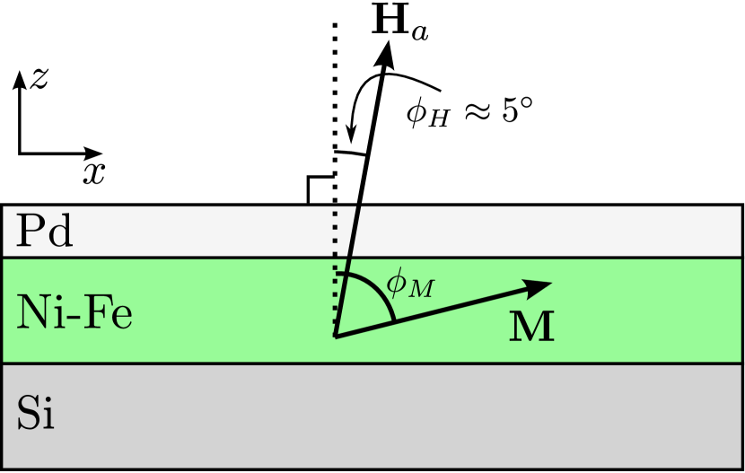
Figure 2: Test sample: Side view of the layer structure of Pd (200 Å) on Ni-Fe alloy (600 Å) on Si substrate. Sample lateral size is 25 mm $\times$ 25 mm. The external applied field is slightly tilted with respect to the surface normal.

For the principal polarized neutron reflectometry measurement of this study, the external magnetic field was applied for the measurement at a small angle to the film surface normal as seen in the figure. The demagnetizing field (shape anisotropy) of the film acts to keep the magnetization in-plane, and for appropriate choices of field strength and angle this dominates over the torque from the applied field, so that the magnetization remains largely in-plane. At the same time, the small in-plane component of the field $H_{x}$ is enough to align the layer into a single domain, pointing mostly along $x$.

This arrangement provides an ideal test of the equations, since there is both a large moment $\mathbf{M}\perp\mathbf{H}$ providing spin-flip scattering, and simultaneously a large $\mathbf{H}$ field which causes Zeeman splitting of those spin-flipped neutrons.

We verified with a vibrating-sample magnetometer measurement that the test sample is indeed magnetically soft with a saturation field in the hard (out-of-plane) direction of about 0.5 T, and at 0.244 T (the applied field for the neutron measurements) the out-of-plane loop is linear with field, suggesting a coherent rotation. This verifies that it is a magnetically soft film with the expected shape anisotropy and no significant domain formation at the neutron measurement condition.

A supplementary reflectometry measurement of the same sample was done in an in-plane saturating field in order to get a good value of the saturation magnetization of the soft magnetic layer. The scattering results from this measurement (not shown) are easily fit to standard models of polarized neutron reflectometry without Zeeman corrections and indicate a saturation internal $B$-field of 0.551 T ($M=439.53$ kA/m) .

5.2 Results

The reflectivity measurements were undertaken at the Polarized Beam Reflectometer instrument (PBR) at the NIST Center for Neutron Research, with supermirror spin polarizer and analyzer and current-coil Mezei-type spin flippers for the incident and reflected beams. In an applied field $\mu_{0}H_{a}=244$ mT at an angle as shown in Fig. 2, for a series of $k_{z(\mathrm{in})}$, all four spin cross-sections were measured at each of the the three outgoing angles corresponding to $(k_{z,F}^{+-})$, $(k_{z,F}^{+-})$, and $(k_{z,F}^{++},k_{z,F}^{--})$. The data for each of those outgoing angles was polarization-corrected and the relevant cross-sections were extracted.

First in Fig. 3 we show a the best fit to the data performed using the freely-available Refl1D [KirbyCOCIS, refl1d] package, but without making corrections for the Zeeman effects. The symbols represent data points with error bars and the lines represent the best fit possible.

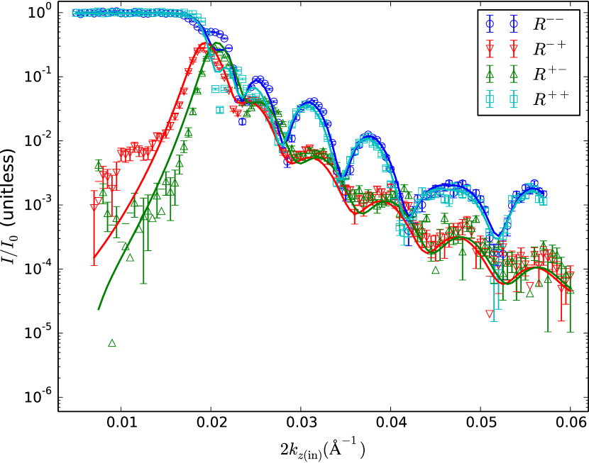
Figure 3: Reflectivity of test sample without including the effects of the Zeeman energy. Data is open symbols, with error bars corresponding to $\pm 1\sigma$ according to counting statistics and resolution function of the instrument; fits are the solid lines (reduced $\chi^{2}$ for this fit is 25.0). Data is parametrized and fit according to $k_{z(\mathrm{in})}$.

We compare this to a fit performed using a modification of the software which includes the changes to the theory described in the first section of this manuscript. Both the data and the fit are presented in Fig. 4.

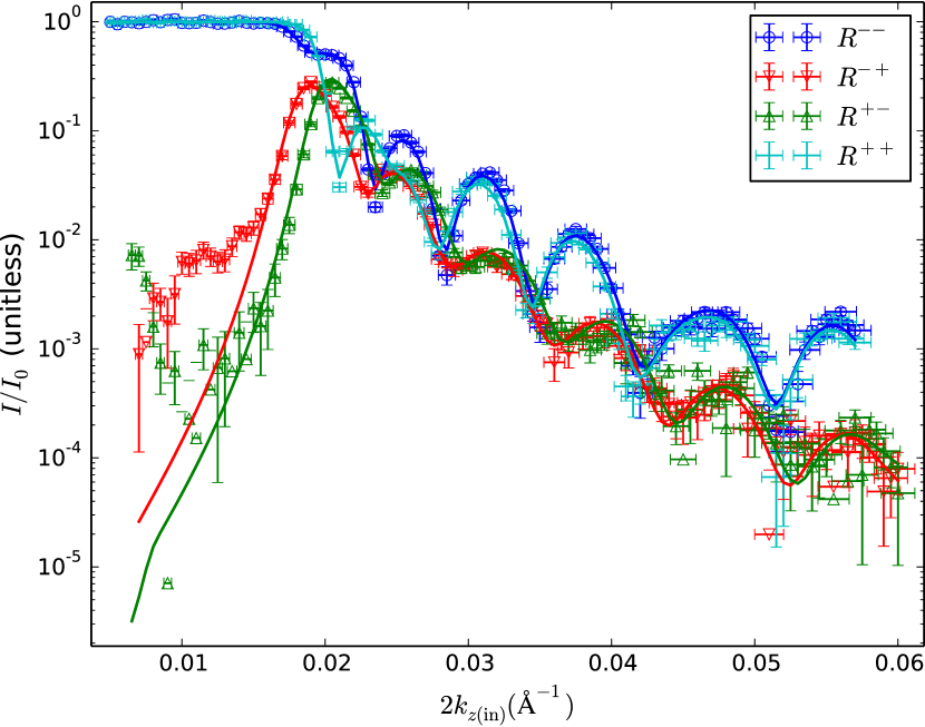
Figure 4: Reflectivity of test sample, in all 4 cross sections, including fit. Data is open symbols, with error bars corresponding to $\pm 1\sigma$ according to counting statistics and resolution function of the instrument; fits are the solid lines (reduced $\chi^{2}$ for this fit is 3.7). Data is parametrized and fit according to $k_{z(\mathrm{in})}$.

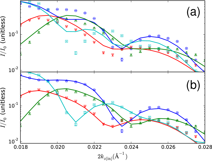
Figure 5: Enlargement of the reflectivity fits near the critical edge. (a) corresponds to the fit without Zeeman corrections in Fig. 3 and (b) corresponds to the corrected fit in Fig. 4. A clear improvement in the quality of the fit is seen. Symbols and lines have the same meanings in this plot as in the originals.

In the uncorrected fit in Fig. 3 we can clearly see that the splitting between the non-spin-flip scattering at low $k_{z\mathrm{(in)}}$ is grossly underestimated in the best-fitting model. In this region the error bars are small due to the strong scattering and this is what leads to the large minimum $\chi^{2}$ value of 25.0 for this fit. An enlargement of this region for comparing corrected vs. uncorrected fits is show in Fig. 5.

By contrast the Zeeman-corrected fit is very good, with a chi-squared value of 3.7. The visible deviations of the spin-flip data from the fit at very low $k_{z\mathrm{(in)}}$ are likely due to issues with the polarization correction (the correction is of the same magnitude as the spin-flip data there), and this does not significantly affect the rest of the fit. In the enlarged plot in Fig. 5(b) this fit clearly reproduces the data near the critical edge. The best fit to the data corresponds to a magnetic scattering length density in the Ni-Fe layer of $\rho_{B}=1.12\times 10^{-6}\textrm{\AA}^{-2}$ and thus $M_{x}=385$ kA/m.

The SLD profiles resulting from the fits in Figs. 3 and 4 (nuclear and magnetic) are shown in Fig. 6 with dotted lines, while the SLD profiles from the corrected fit are shown with solid lines. The difference between the profiles is most prevalent in the region of the capping layer, where the uncorrected fit gives an unphysically low value of nuclear SLD of the Pd capping layer (2.7 Å^-1 rather than the expected value of 4.1 Å^-1,) and an unrealistically low roughness for the top interface, where one would expect the top interface to have similar roughness to the interface immediately below.

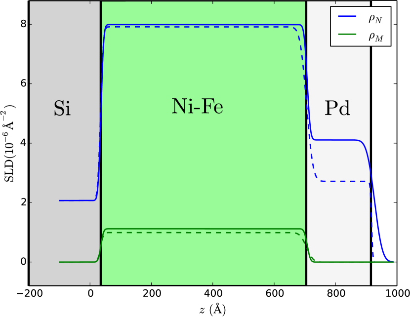
Figure 6: Scattering length density profile (SLD) corresponding to the fits shown in Fig. 4 (solid line) and Fig. 3 (dashed line). $\rho_{N}$ and $\rho_{M}$ refer to the nuclear and magnetic scattering length densities respectively in blue and green. Profile is overlaid on a color-coded diagram of the sample structure as seen in Fig. 2 for reference.

The out-of-plane component of $\vec{M}$ for a system with uniaxial anisotropy arising from the demagnetization field is expected to be linearly dependent (when coherently rotating across the entire sample) on an applied out-of-plane field, reaching the saturation value at $H_{k}=4\pi M_{S}$. In our case $M_{z}\approx(H_{a}/H_{k})M_{S}=(0.244/0.551)M_{S}$, and since $M_{z}=M_{S}\cos\phi$ and $M_{x}=M_{S}\sin\phi$, we can extract an expected value of the in-plane magnetization $M_{x}\approx 394$ kA/m, which agrees well with the fit value of 385 kA/m.

The most striking feature of the scattering in Fig. 4 is the large splitting between the non-spin-flip reflectivities $R^{++},R^{--}$ at low $k_{z(\mathrm{in})}$, but which disappears at higher $k_{z}$. This is a signature of the Zeeman effect, which will be most pronounced when the Zeeman energy is comparable to the kinetic energy along the scattering direction.

The best indication that this splitting is a result of the Zeeman effect is to compare with data fitted to a model with no Zeeman energy included; this is shown in Fig. 3.

In Figs. 4 and 3 there is an apparent horizontal shift between the two spin-flip reflectivities. This is entirely due to the choice of plotting that data as a function of $2k_{z(\mathrm{in})}$. If we had chosen to plot vs. the total momentum transfer $Q$ the features would be mostly aligned, but the advantage of plotting it this way is that the scattering sum rules are more apparent; for an incident beam $I^{-}$ at low angles where the scattering is strong, we can clearly see the non-spin-flip reflectivity $R^{--}$ has a dip when $R^{-+}$ has a peak (a similar correspondence is seen between $R^{++}$ and $R^{+-}$.)

6 Conclusions

We have described a procedure for measuring polarized neutron reflectivity in high fields, including important changes to the modeling and instrument configuration due to Zeeman shifts in the energy and angle of spin-flip scattered neutrons. These considerations will be important for characterization of thin films with large magnetic anisotropy, which are a component of a growing number of technologically relevant systems.

A data-modeling package with the necessary modifications for this type of measurement was demonstrated to provide accurate quantitative fits of a test system, and this software is now readily available to the research community [refl1d]. The deviations from non-Zeeman-corrected polarized specular neutron modeling are most pronounced where the spin-flip scattering is most intense.

Acknowledgements Y. Liu is supported by the Division of Scientific User Facilities of the Office of Basic Energy Sciences, US Department of Energy.

References

- [1] \harvarditem[Dura et al.]Dura, Pierce, Majkrzak, Maliszewskyj, McGillivray, Lösche, O’Donovan, Mihailescu, Perez-Salas \harvardand Worcester2006dura2006and Dura, J., Pierce, D., Majkrzak, C., Maliszewskyj, N., McGillivray, D., Lösche, M., O’Donovan, K., Mihailescu, M., Perez-Salas, U. \harvardand Worcester, D. \harvardyearleft2006\harvardyearright. Review of scientific instruments, \volbf77, 074301.
- [2] \harvarditem[Felcher et al.]Felcher, Adenwalla, De Haan \harvardand Van Well1995felcher1995zeeman Felcher, G., Adenwalla, S., De Haan, V. \harvardand Van Well, A. \harvardyearleft1995\harvardyearright. Nature, \volbf377(6548), 409–410.
- [3] \harvarditem[Felcher et al.]Felcher, Adenwalla, De Haan \harvardand Van Well1996felcher1996observation Felcher, G., Adenwalla, S., De Haan, V. \harvardand Van Well, A. \harvardyearleft1996\harvardyearright. Physica B: Condensed Matter, \volbf221(1), 494–499.
-
[4]
\harvarditemKienzle2015refl1d
Kienzle, P., \harvardyearleft2015\harvardyearright.
Refl1d package for fitting reflectivity data.
\harvardurlhttp://ncnr.nist.gov/reflpak -
[5]
\harvarditem[Kirby et al.]Kirby, Kienzle, Maranville, Berk, Krycka,
Heinrich \harvardand Majkrzak2012KirbyCOCIS
Kirby, B., Kienzle, P., Maranville, B., Berk, N., Krycka, J., Heinrich, F.
\harvardand Majkrzak, C. \harvardyearleft2012\harvardyearright.
Current Opinion in Colloid & Interface Science,
\volbf17(1), 44 – 53.
\harvardurlhttp://www.sciencedirect.com/science/article/pii/ S1359029411001488 - [6] \harvarditem[Kozhevnikov et al.]Kozhevnikov, Ott \harvardand Radu2012kozhevnikov2012data Kozhevnikov, S., Ott, F. \harvardand Radu, F. \harvardyearleft2012\harvardyearright. Journal of Applied Crystallography, \volbf45(4), 814–825.
- [7] \harvarditem[van de Kruijs et al.]van de Kruijs, Fredrikze, Rekveldt, van Well, Nikitenko \harvardand Syromyatnikov2000vandeKruijs2000189 van de Kruijs, R., Fredrikze, H., Rekveldt, M., van Well, A., Nikitenko, Y. \harvardand Syromyatnikov, V. \harvardyearleft2000\harvardyearright. Physica B: Condensed Matter, \volbf283(1-3), 189–193.
-
[8]
\harvarditem[Liu et al.]Liu, te Velthuis, Jiang, Choi, Bader, Parizzi,
Ambaye \harvardand Lauter2011PhysRevB.83.174418
Liu, Y., te Velthuis, S. G. E., Jiang, J. S., Choi, Y., Bader, S. D., Parizzi,
A. A., Ambaye, H. \harvardand Lauter, V. \harvardyearleft2011\harvardyearright.
Phys. Rev. B, \volbf83, 174418.
\harvardurlhttp://link.aps.org/doi/10.1103/PhysRevB.83.174418 - [9] \harvarditem[Majkrzak et al.]Majkrzak, O’Donovan \harvardand Berk2006PNRMajkrzakChapter Majkrzak, C., O’Donovan, K. \harvardand Berk, N. \harvardyearleft2006\harvardyearright. In Neutron scattering from magnetic materials, edited by T. Chatterji, pp. 397–471. Elsevier Science.
- [10]