Discrete-Time Approximations of Fliess Operators

Abstract

A convenient way to represent a nonlinear input-output system in control theory is via a Chen-Fliess functional expansion or Fliess operator. The general goal of this paper is to describe how to approximate Fliess operators with iterated sums and to provide accurate error estimates for two different scenarios, one where the series coefficients are growing at a local convergence rate, and the other where they are growing at a global convergence rate. In each case, it is shown that the error estimates are achievable in the sense that worst case inputs can be identified which hit the error bound. The paper then focuses on the special case where the operators are rational, i.e., they have rational generating series. It is shown in this situation that the iterated sum approximation can be realized by a discrete-time state space model which is a rational function of the input and state affine. In addition, this model comes from a specific discretization of the bilinear realization of the rational Fliess operator.

1 Introduction

A convenient way to represent a nonlinear input-output system in control theory is via a Chen-Fliess functional expansion or Fliess operator Fliess_81 ; Fliess_83 ; Isidori_95 . This series of weighted iterated integrals of the input functions exhibits considerable algebraic structure that can be used, for example, to describe system interconnections Gray-et-al_SCL14 ; Gray-Li_05 and to perform system inversion Gray-et-al_CDC15 ; Gray-et-al_Auto14 . On the other hand, in the context of numerical simulation and approximation, it is less clear how such a representation can be utilized efficiently. In guidance applications, for example, piecewise constant approximations of the input have been used in combination with a truncated version of the series to find acceptable solutions to specific problems He-etal_2013 ; Yao-etal_2008 . But no a priori error estimates are provided for this approach. Passing through a discrete-time approximation of an equivalent state space model is also an option, but not every Fliess operator is realizable by a system of differential equations Fliess_83 . One hint to the general problem of approximating Fliess operators was provided by Grüne and Kloeden in Grune-Kloeden_01 , where it was shown that iterated integrals can be well approximated by iterated sums. But there is a considerable jump in going from approximating a single iterated integral to approximating an infinite sum of such integrals. In particular, the error estimates for each iterated integral have to be precise enough to yield an accurate error estimate for the whole operator. Further complicating the picture is the fact that in practice only finite sums can be computed. So an independent truncation error also has to be accounted for.

The general goal of this paper is to describe how to approximate Fliess operators with iterated sums and to provide accurate error estimates for different scenarios. The starting point is to develop a refinement of the error estimate in (Grune-Kloeden_01, , Lemma 2) for a single iterated integral. This is done largely using Chen’s Lemma Chen_52 . After this, two specific cases are considered, one in which the series coefficients are growing at a local convergence rate, and the other where they are growing at a global convergence rate Gray-Wang_SCL02 . Each case yields different error estimates, and several simulation examples are given to demonstrate the results. In particular, it is shown that the error estimates are achievable in the sense that worst case inputs can be identified which hit the error bound. The paper then focuses on the special case where the operators are rational, i.e., have rational generating series Berstel-Reutenauer_88 . In particular, it is shown that the iterated sum approximation of a rational Fliess operator can be realized by a discrete-time state space model which is a rational function of the input and state affine. This means that the approximating iterated sums do not have to be computed explicitly but can be done implicitly via a difference equation. In which case, the truncation error can be completely avoided. It is also shown that this difference equation approach can be viewed in terms of a specific discretization of a continuous-time bilinear realization of the rational Fliess operator.

The paper is organized as follows. First some preliminaries on Fliess operators, Chen’s Lemma, and rational series are given to set the notation and terminology. Next the notion of a discrete-time Fliess operator is developed in Section 3. Then the main approximation theorems are given in Section 4. In the subsequent section, the material concerning rational operators is presented. The conclusions of the paper are given in the final section.

2 Preliminaries

A finite nonempty set of noncommuting symbols $X=\{x_{0},x_{1},$ $\ldots,x_{m}\}$ is called an alphabet. Each element of $X$ is called a letter, and any finite sequence of letters from $X$, $\eta=x_{i_{1}}\cdots x_{i_{k}}$, is called a word over $X$. The length of $\eta$, $\left|\eta\right|$, is the number of letters in $\eta$. The set of all words with length $k$ is denoted by $X^{k}$. The set of all words including the empty word, $\emptyset$, is designated by $X^{\ast}$. It forms a monoid under catenation. The set $\eta X^{\ast}$ is comprised of all words with the prefix $\eta$. Any mapping $c:X^{\ast}\rightarrow{\mathbb{R}}^{\ell}$ is called a formal power series. The value of $c$ at $\eta\in X^{\ast}$ is written as $(c,\eta)$ and called the coefficient of $\eta$ in $c$. Typically, $c$ is represented as the formal sum $c=\sum_{\eta\in X^{\ast}}(c,\eta)\eta.$ If the constant term $(c,\emptyset)=0$ then $c$ is said to be proper. The support of $c$, ${\rm supp}(c)$, is the set of all words having nonzero coefficients. The collection of all formal power series over $X$ is denoted by ${\mathbb{R}}^{\ell}\langle\langle X\rangle\rangle$. The subset of polynomials is written as ${\mathbb{R}}^{\ell}\langle X\rangle$. Each set forms an associative ${\mathbb{R}}$-algebra under the catenation product and a commutative and associative ${\mathbb{R}}$-algebra under the shuffle product, denoted here by ${\scriptscriptstyle\;\sqcup\sqcup\;}$. The latter is the ${\mathbb{R}}$-bilinear extension of the shuffle product of two words, which is defined inductively by

$$(x_{i}\eta){\scriptscriptstyle\;\sqcup\sqcup\;}(x_{j}\xi)=x_{i}(\eta{\scriptscriptstyle\;\sqcup\sqcup\;}(x_{j}\xi))+x_{j}((x_{i}\eta){\scriptscriptstyle\;\sqcup\sqcup\;}\xi)$$

with $\eta{\scriptscriptstyle\;\sqcup\sqcup\;}\emptyset=\emptyset{\scriptscriptstyle\;\sqcup\sqcup\;}\eta=\eta$ for all $\eta,\xi\in X^{\ast}$ and $x_{i},x_{j}\in X$.

2.1 Fliess Operators

One can formally associate with any series $c\in\mbox{${\mathbb{R}}^{\ell}\langle\langle X\rangle\rangle$}$ a causal $m$-input, $\ell$-output operator, $F_{c}$, in the following manner. Let $\mathfrak{p}\geq 1$ and $t_{0}<t_{1}$ be given. For a Lebesgue measurable function $u:[t_{0},t_{1}]\rightarrow{\mathbb{R}}^{m}$, define $\|u\|_{\mathfrak{p}}=\max\{\|u_{i}\|_{\mathfrak{p}}:\ 1\leq i\leq m\}$, where $\|u_{i}\|_{\mathfrak{p}}$ is the usual $L_{\mathfrak{p}}$-norm for a measurable real-valued function, $u_{i}$, defined on $[t_{0},t_{1}]$. Let $L^{m}_{\mathfrak{p}}[t_{0},t_{1}]$ denote the set of all measurable functions defined on $[t_{0},t_{1}]$ having a finite $\|\cdot\|_{\mathfrak{p}}$ norm and $B_{\mathfrak{p}}^{m}(R)[t_{0},t_{1}]:=\{u\in L_{\mathfrak{p}}^{m}[t_{0},t_{1}]:\|u\|_{\mathfrak{p}}\leq R\}$. Assume $C[t_{0},t_{1}]$ is the subset of continuous functions in $L_{1}^{m}[t_{0},t_{1}]$. Define inductively for each $\eta\in X^{\ast}$ the map $E_{\eta}:L_{1}^{m}[t_{0},t_{1}]\rightarrow C[t_{0},t_{1}]$ by setting $E_{\emptyset}[u]=1$ and letting

$$E_{x_{i}\bar{\eta}}[u](t,t_{0})=\int_{t_{0}}^{t}u_{i}(\tau)E_{\bar{\eta}}[u](\tau,t_{0})\,d\tau,$$

where $x_{i}\in X$, $\bar{\eta}\in X^{\ast}$, and $u_{0}=1$. The input-output operator corresponding to $c$ is the Fliess operator

$$F_{c}[u](t)=\sum_{\eta\in X^{\ast}}(c,\eta)\,E_{\eta}[u](t,t_{0}).$$ (1)

If there exist real numbers $K_{c},M_{c}>0$ such that

$$\left|(c,\eta)\right|\leq K_{c}M_{c}^{|\eta|}|\eta|!,\;\;\forall\eta\in X^{\ast},$$ (2)

then $F_{c}$ constitutes a well defined mapping from $B_{\mathfrak{p}}^{m}(R)[t_{0},$ $t_{0}+T]$ into $B_{\mathfrak{q}}^{\ell}(S)[t_{0},\,t_{0}+T]$ provided $\bar{R}:=\max\{R,T\}<1/M_{c}(m+1)$, and the numbers $\mathfrak{p},\mathfrak{q}\in[1,\infty]$ are conjugate exponents, i.e., $1/\mathfrak{p}+1/\mathfrak{q}=1$ Gray-Wang_SCL02 . (Here, $\left|z\right|:=\max_{i}\left|z_{i}\right|$ when $z\in{\mathbb{R}}^{\ell}$.) In this case, the operator $F_{c}$ is said to be locally convergent (LC), and the set of all series satisfying (2) is denoted by ${\mathbb{R}}^{\ell}_{LC}\langle\langle X\rangle\rangle$. When $c$ satisfies the more stringent growth condition

$$\left|(c,\eta)\right|\leq K_{c}M_{c}^{|\eta|},\;\;\forall\eta\in X^{\ast},$$ (3)

the series (1) defines an operator from the extended space $L^{m}_{\mathfrak{p},e}(t_{0})$ into $C[t_{0},\infty)$, where

$$L^{m}_{\mathfrak{p},e}(t_{0}):=\{u:[t_{0},\infty)\rightarrow{\mathbb{R}}^{m}:u_{[t_{0},t_{1}]}\in L_{\mathfrak{p}}^{m}[t_{0},t_{1}],\forall t_{1}\in(t_{0},\infty)\},$$

and $u_{[t_{0},t_{1}]}$ denotes the restriction of $u$ to $[t_{0},t_{1}]$ Gray-Wang_SCL02 . In this case, the operator is said to be globally convergent (GC), and the set of all series satisfying (3) is designated by ${\mathbb{R}}^{\ell}_{GC}\langle\langle X\rangle\rangle$.

2.2 Chen’s Lemma

For a fixed $u$ consider a series in ${\mathbb{R}}\langle\langle X\rangle\rangle$ of the form $P[u]=\sum_{\eta\in X^{\ast}}\eta E_{\eta}[u]$, which is often referred to as a Chen series. Given two functions $(u,v)\in L_{1}^{m}[t_{a},t_{b}]\times L_{1}^{m}[t_{c},t_{d}]$, their durations are taken to be $t_{b}-t_{a}\geq 0$ and $t_{d}-t_{c}\geq 0$, respectively, and the functions are not defined outside their corresponding intervals. The catenation of $u$ and $v$ at $\tau\in[t_{a},t_{b}]$ is understood to be

$$(v\#_{\tau}u)(t)=\left\{\begin{array}[]{ccl}u(t)&:&t_{a}\leq t\leq\tau\\ v((t-\tau)+t_{c})&:&\tau<t\leq\tau+(t_{d}-t_{c})\end{array}\right.$$

(see Figure 1).

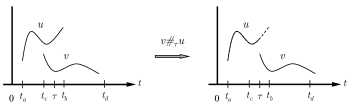
Figure 1: The catenation of two inputs $u$ and $v$ at $t=\tau$.

It is easily verified that $L_{1,e}^{m}(0)$ is a monoid under the catenation operator. The identity element in this case is denoted by $\mathbf{0}$ and is equivalent to the set of functions having exactly zero duration. The following lemma is due to Chen Chen_52 .

Lemma 1

(Chen’s Lemma) If $(u,v)\in L_{1}^{m}[0,T_{1}]\times L_{1}^{m}[0,T_{2}]$ and $(t_{1},t_{2})\in[0,T_{1}]\times[0,T_{2}]$ then

$$P[v](t_{2})P[u](t_{1})=P[v\#_{t_{1}}u](t_{2}+t_{1}).\\$$

So in essence $P:L_{1,e}^{m}(0)\rightarrow\mbox{${\mathbb{R}}\langle\langle X\rangle\rangle$}$ acts as a monoid morphism, where ${\mathbb{R}}\langle\langle X\rangle\rangle$ is viewed as a monoid under the catenation product.

2.3 Rational Formal Power Series

A brief summary of rational and recognizable formal power series is useful. The treatment here is based largely on Berstel-Reutenauer_88 .

A series $c\in\mbox{${\mathbb{R}}\langle\langle X\rangle\rangle$}$ is called invertible if there exists a series $c^{-1}\in\mbox{${\mathbb{R}}\langle\langle X\rangle\rangle$}$ such that $cc^{-1}=c^{-1}c=1$. In the event that $c$ is not proper, it is always possible to write

$$c=(c,\emptyset)(1-c^{\prime}),$$

where $(c,\emptyset)$ is nonzero, and $c^{\prime}\in\mbox{${\mathbb{R}}\langle\langle X\rangle\rangle$}$ is proper. It then follows that

$$c^{-1}=\frac{1}{(c,\emptyset)}(1-c^{\prime})^{-1}=\frac{1}{(c,\emptyset)}(c^{\prime})^{\ast},$$

where

$$(c^{\prime})^{\ast}:=\sum_{i=0}^{\infty}(c^{\prime})^{i}.$$

In fact, $c$ is invertible if and only if $c$ is not proper. Now let $S$ be a subalgebra of the ${\mathbb{R}}$-algebra ${\mathbb{R}}\langle\langle X\rangle\rangle$ with the catenation product. $S$ is said to be rationally closed when every invertible $c\in S$ has $c^{-1}\in S$ (or equivalently, every proper $c^{\prime}\in S$ has $(c^{\prime})^{\ast}\in S$). The rational closure of any subset $E\subset\mbox{${\mathbb{R}}\langle\langle X\rangle\rangle$}$ is the smallest rationally closed subalgebra of ${\mathbb{R}}\langle\langle X\rangle\rangle$ containing $E$.

Definition 1

A series $c\in\mbox{${\mathbb{R}}\langle\langle X\rangle\rangle$}$ is rational if it belongs to the rational closure of ${\mathbb{R}}\langle X\rangle$.

It turns out that an entirely different characterization of a rational series is possible using the following concept.

Definition 2

A linear representation of a series $c\in\mbox{${\mathbb{R}}\langle\langle X\rangle\rangle$}$ is any triple $(\mu,\gamma,\lambda)$, where

$$\mu:X^{\ast}\rightarrow{\mathbb{R}}^{n\times n}$$

is a monoid morphism, and $\gamma,\lambda^{T}\in{\mathbb{R}}^{n\times 1}$ are such that

$$(c,\eta)=\lambda\mu(\eta)\gamma,\;\forall\eta\in X^{\ast}.$$

The integer $n$ is the dimension of the representation.

Definition 3

A series $c\in\mbox{${\mathbb{R}}\langle\langle X\rangle\rangle$}$ is called recognizable if it has a linear representation.

Theorem 2.1

(Schützenberger) A formal power series is rational if and only if it is recognizable.

The next concept provides an explicit way of constructing a linear representation of a rational series. Define for any $x_{i}\in X$, the left-shift operator, $x_{i}^{-1}(\cdot)$, on $X^{\ast}$ by $x_{i}^{-1}(x_{i}\eta)=\eta$ with $\eta\in X^{\ast}$ and zero otherwise. Higher order shifts are defined inductively via $(x_{i}\xi)^{-1}(\cdot)=\xi^{-1}x_{i}^{-1}(\cdot)$, where $\xi\in X^{\ast}$. The left-shift operator is assumed to act linearly on ${\mathbb{R}}\langle\langle X\rangle\rangle$.

Definition 4

A subset $V\subset\mbox{${\mathbb{R}}\langle\langle X\rangle\rangle$}$ is called stable when $\xi^{-1}(c)\in V$ for all $c\in V$ and $\xi\in X^{\ast}$.

Theorem 2.2

A series $c\in\mbox{${\mathbb{R}}\langle\langle X\rangle\rangle$}$ is rational/recognizable if and only if there exists a stable finite dimensional ${\mathbb{R}}$-vector subspace of ${\mathbb{R}}\langle\langle X\rangle\rangle$ containing $c$.

3 Discrete-Time Fliess Operators

Let $u\in L_{1}^{m}[0,T]$ for some finite $T>0$. Following Grune-Kloeden_01 , select some integer $L\geq 1$ and with $\Delta:=T/L$ define the sequence

$$\hat{u}_{i}(N)=\int_{(N-1)\Delta}^{N\Delta}u_{i}(t)\,dt,\;\;i=0,1,\ldots,m$$ (4)

where $N\in[1,L]$. Observe in particular that $\hat{u}_{0}(N)=\Delta$ since $u_{0}=1$. The corresponding iterated sum for any $x_{i}\in X$ and $\eta\in X^{\ast}$ is defined inductively by

$$S_{x_{i}\eta}[\hat{u}](N)=\sum_{k=1}^{N}\hat{u}_{i}(k)S_{\eta}[\hat{u}](k)$$

with $S_{\emptyset}[\hat{u}](N):=1$. The following lemma gives an alternative description of $S_{\eta}$ which will be useful later.

Lemma 2

For any $N\in[1,L]$ and $\eta\in X^{\ast}$

$$S_{\eta}[\hat{u}](N)=\Delta^{\left|\eta\right|}\sum_{\xi_{N}\cdots\xi_{1}=\eta}u_{\xi_{N}}(N)\cdots u_{\xi_{1}}(1),$$

where $u_{i}(k):=\hat{u}_{i}(k)/\Delta$, $u_{x_{i_{1}}\cdots x_{i_{r}}}(k):=u_{i_{1}}(k)\cdots u_{i_{r}}(k)$, $u_{\emptyset}(k):=1$, and the summation is over all partitions of $\eta$ having N subwords $\xi_{k}\in X^{\ast}$ (so some subwords can be empty).

Proof:  The proof is by induction on the length of $\eta$. For the empty word the equality holds trivially. When $\eta=x_{i}$ observe that

$$S_{x_{i}}[\hat{u}](N)=\sum_{k=1}^{N}\hat{u}_{i}(k)=\Delta\sum_{k=1}^{N}u_{i}(k)=\Delta\sum_{\xi_{N}\cdots\xi_{1}=x_{i}}u_{\xi_{N}}(N)\cdots u_{\xi_{1}}(1).$$

Now assume the claim holds for all words up to length $j\geq 0$. If $\eta\in X^{j}$ then

$$S_{x_{i}\eta}[\hat{u}](N) =\sum_{k=1}^{N}\hat{u}_{i}(k)S_{\eta}[\hat{u}](k)=\sum_{k=1}^{N}\Delta u_{i}(k)\Delta^{j}\sum_{\xi_{k}\cdots\xi_{1}=\eta}u_{\xi_{k}}(k)\cdots u_{\xi_{1}}(1)$$

$$=\Delta^{j+1}\sum_{\xi_{N}\cdots\xi_{1}=x_{i}\eta}u_{\xi_{N}}(N)\cdots u_{\xi_{1}}(1),$$

which proves the lemma.  

The next definition provides the main class of discrete-time approximators used throughout the paper. In the most general context, the set of admissible inputs will be drawn from the real sequence space $l_{\infty}^{m+1}[N_{0}]:=\{\hat{u}=(\hat{u}(N_{0}),\hat{u}(N_{0}+1),\ldots):\left|\hat{u}(N)\right|<\hat{R}_{\hat{u}}<\infty,\,\forall N\geq N_{0}\}$, where $\left|\hat{u}(N)\right|:=\max_{i=0,1,\ldots,m}\left|\hat{u}_{i}(N)\right|$. In which case, $\|\hat{u}\|_{\infty}:=\sup_{N\geq N_{0}}\left|\hat{u}(N)\right|$ is always finite. To be consistent with (4), it is assumed throughout that $\hat{u}_{0}$ is a constant input. Define a ball of radius $\hat{R}$ in $l_{\infty}^{m+1}[N_{0}]$ as $B_{\infty}^{m+1}[N_{0}]$ $(\hat{R})=\{\hat{u}\in l_{\infty}^{m+1}[N_{0}]:\|\hat{u}\|_{\infty}\leq\hat{R}\}$. The subset of finite sequences over $[N_{0},N_{f}]$ is denoted by $B_{\infty}^{m+1}[N_{0},N_{f}](\hat{R})$.

Definition 5

For any $c\in\mbox{${\mathbb{R}}^{\ell}\langle\langle X\rangle\rangle$}$, the corresponding discrete-time Fliess operator defined on $l_{\infty}^{m+1}[1]$ is

$$\hat{y}(N)=\hat{F}_{c}[\hat{u}](N)=\sum_{\eta\in X^{\ast}}(c,\eta)S_{\eta}[\hat{u}](N).$$ (5)

Before considering the approximation problem, it is necessary to introduce various sufficient conditions for convergence of such operators. The following lemma is essential.

Lemma 3

If $\hat{u}\in B_{\infty}^{m+1}[1](\hat{R})$ then for any $\eta\in X^{\ast}$

$$\left|S_{\eta}[\hat{u}](N)\right|\leq\hat{R}^{\left|\eta\right|}{N-1+\left|\eta\right|\choose\left|\eta\right|}.\\$$

Proof:  If $\eta=x_{i_{j}}\cdots x_{i_{1}}$ then observe for any $N\geq 1$

$$\left|S_{\eta}[\hat{u}](N)\right| =\left|\sum_{k_{j}=1}^{N}\hat{u}_{i_{j}}(k_{j})\sum_{k_{j-1}=1}^{k_{j}}\hat{u}_{i_{j-1}}(k_{j-1})\cdots\sum_{k_{1}=1}^{k_{2}}\hat{u}_{i_{1}}(k_{1})\right|$$

$$\leq\sum_{k_{j}=1}^{N}\left|\hat{u}_{i_{j}}(k_{j})\right|\sum_{k_{j-1}=1}^{k_{j}}\left|\hat{u}_{i_{j-1}}(k_{j-1})\right|\cdots\sum_{k_{1}=1}^{k_{2}}\left|\hat{u}_{i_{1}}(k_{1})\right|$$

$$\leq\hat{R}^{\left|\eta\right|}\sum_{k_{j}=1}^{N}\sum_{k_{j-1}=1}^{k_{j}}\cdots\sum_{k_{1}=1}^{k_{2}}1$$

$$=\hat{R}^{\left|\eta\right|}{N-1+\left|\eta\right|\choose\left|\eta\right|},$$

using the fact that the final nested sum above has ${N-1+\left|\eta\right|\choose\left|\eta\right|}$ terms Butler-Karasik_10 .  

Since the upper bound on $\left|S_{\eta}[\hat{u}](N)\right|$ in this lemma is achievable on $B_{\infty}^{m+1}[1](\hat{R})$, it is not difficult to see that when the generating series $c$ satisfies the growth bound (2), the series (5) defining $\hat{F}_{c}$ can diverge. For example, if $(c,\eta)=K_{c}M_{c}^{\left|\eta\right|}\left|\eta\right|!$ for all $\eta\in X^{\ast}$, and $\hat{u}$ is such a maximizing input then

$$\hat{F}[\hat{u}](N) =K_{c}\sum_{\eta\in X^{\ast}}M_{c}^{\left|\eta\right|}\left|\eta\right|!\hat{R}^{\left|\eta\right|}{N-1+\left|\eta\right|\choose\left|\eta\right|}$$

$$=K_{c}\sum_{j=0}^{\infty}(M_{c}(m+1)\hat{R})^{j}((N-1+j)\cdots(N+1)N),$$

which will diverge even if $M_{c}(m+1)\hat{R}<1$. The next theorem shows that this problem is averted when $c$ satisfies the stronger growth condition (3).

Theorem 3.1

Suppose $c\in\mbox{${\mathbb{R}}^{\ell}\langle\langle X\rangle\rangle$}$ has coefficients which satisfy (3). Then there exists a real number $\hat{R}>0$ and an integer $L\geq 1$ such that for each $\hat{u}\in B_{\infty}^{m+1}[1,L](\hat{R})$, the series (5) converges absolutely and uniformly on $[1,L]$.

Proof:  Fix $L\geq 1$ and select any $N\in[1,L]$. In light of Lemma 3, if $\left|\eta\right|\gg N$ then

$$\left|S_{\eta}[\hat{u}](N)\right|\lesssim\hat{R}^{\left|\eta\right|}\frac{1}{(N-1)!}.$$

From the assumed coefficient bound it follows that

$$\left|\hat{F}_{c}(\hat{u})(N)\right| \leq\sum_{j=0}^{\infty}\sum_{\eta\in X^{j}}\left|(c,\eta)\right|\left|S_{\eta}[\hat{u}](N)\right|\lesssim\sum_{j=0}^{\infty}K_{c}(M_{c}(m+1))^{j}\,\hat{R}^{j}\frac{1}{(N-1)!}$$

$$=\frac{1}{(N-1)!}\frac{K_{c}}{1-M_{c}(m+1)\hat{R}},$$

provided $\hat{R}<1/M_{c}(m+1)$. Since $\hat{u}_{0}$ is constant on $[1,L]$, an upper bound on $L$ is also implied.  

The final convergence theorem shows that the restriction on the norm of $\hat{u}$ can be removed if an even more stringent growth condition is imposed on $c$.

Theorem 3.2

Suppose $c\in\mbox{${\mathbb{R}}^{\ell}\langle\langle X\rangle\rangle$}$ has coefficients which satisfy

$$\left|(c,\eta)\right|\leq K_{c}M_{c}^{\left|\eta\right|}\frac{1}{\left|\eta\right|!},\;\;\eta\in X^{\ast}$$

for some real numbers $K_{c},M_{c}>0$. Then for every $\hat{u}\in l_{\infty}^{m+1}[1]$, the series (5) converges absolutely and uniformly on $[1,\infty)$.

Proof:  Following the same argument as in the proof of the previous theorem, it is clear for any $\hat{u}\in l_{\infty}^{m+1}[1]$ and $N\geq 1$ that

$$\left|\hat{F}_{c}(\hat{u})(N)\right|\lesssim\sum_{j=0}^{\infty}K_{c}(M_{c}(m+1))^{j}\frac{1}{j!}\,\|\hat{u}\|_{\infty}^{j}\frac{1}{(N-1)!}=\frac{K_{c}}{(N-1)!}{\rm e}^{M_{c}(m+1)\|\hat{u}\|_{\infty}}.$$

 

Assuming the analogous definitions for local and global convergence of the operator $\hat{F}_{c}$, note the incongruence between the convergence conditions for continuous-time and discrete-time Fliess operators as summarized in Table 1. In each case, for a fixed $c$, the sense in which $\hat{F}_{c}$ converges is weaker than that for $F_{c}$. This is not entirely surprising given that the input $\hat{u}$ in the approximation setting is viewed as the increments of the integral of $u$ rather than $u$ itself. But the real source of this dichotomy is the observation in Lemma 3 that iterated sums of $\hat{u}$ do not grow as a function of word length like $1/\left|\eta\right|!$, which is the case for iterated integrals. As shown in the next section, however, this difference in convergence behavior does not provide any serious impediment to using discrete-time Fliess operators as approximators for their continuous-time counterparts.

Table 1: Summary of convergence conditions for $F_{c}$ and $\hat{F}_{c}$.

growth rate	$F_{c}$	$\hat{F}_{c}$
$\left|(c,\eta)\right|\leq K_{c}M_{c}^{|\eta|}|\eta|!$	LC	divergent
$\left|(c,\eta)\right|\leq K_{c}M_{c}^{|\eta|}$	GC	LC
$\left|(c,\eta)\right|\leq K_{c}M_{c}^{|\eta|}\frac{1}{|\eta|!}$	at least GC	GC

4 Approximating Fliess Operators

4.1 Iterated Integrals

The starting point for the approximation theory is the observation that $E_{x_{i}}[u](T,0)=S_{x_{i}}[\hat{u}](L)$ for all $x_{i}\in X$ and the assertion of Grüne and Kloeden that for any $\eta\in X^{\ast}$ with $|\eta|\geq 2$

$$S_{\eta}[\hat{u}](L)=E_{\eta}[u](T,0)+O\left(\frac{T^{|\eta|}}{L}\right)$$

(Grune-Kloeden_01, , Lemma 2). The following theorem gives an explicit error bound along these lines.

Theorem 4.1

Let $u\in L_{1}^{m}[0,T]$ for some finite $T>0$. Select integer $L\geq 1$, set $\Delta:=T/L$, and define the sequence $\hat{u}$ as in (4). For any $\eta\in X^{\ast}$ it follows that if $L\gg\left|\eta\right|\geq 2$ then

$$\left|S_{\eta}[\hat{u}](L)-E_{\eta}[u](T,0)\right|\lesssim\frac{T^{\left|\eta\right|}}{L}\frac{\|\hat{u}/\Delta\|_{\infty}^{\left|\eta\right|}}{2(\left|\eta\right|-2)!}.\\$$

Proof:  Since the input sequence $\hat{u}$ is computed exactly from the integration of $u$, there is no loss of generality in the computation of $S_{\eta}[\hat{u}](L)$ if one assumes a priori that $u$ is a piecewise constant input taking values $u_{i}(t):=\hat{u}_{i}(N)/\Delta$ when $t\in[(N-1)\Delta,N\Delta)$ for $i=0,1,\ldots,m$. In addition, it was shown in (Gray-Wang_SCL02, , Lemma 2.1) for any $u\in L_{1}[0,T]$ that

$$\left|E_{\eta}[u](N\Delta,(N-1)\Delta)\right|\leq\frac{U_{0}^{\left|\eta\right|_{x_{0}}}\cdots{U_{m}^{\left|\eta\right|_{x_{m}}}}}{\left|\eta\right|_{x_{0}}!\cdots\left|\eta\right|_{x_{m}}!},$$ (6)

where $U_{i}:=\int_{(N-1)\Delta}^{N\Delta}\left|u_{i}(\tau)\right|\,d\tau$, and $\left|\eta\right|_{x_{k}}$ denotes the number of times the letter $x_{k}$ appears in $\eta$. This upper bound is achieved when each $u_{i}$ is constant over $[(N-1)\Delta,N\Delta)$. Thus, the worst case error between $E_{\eta}[u](T)$ and $S_{\eta}[\hat{u}](L)$ occurs for piecewise constant inputs. Applying Chen’s Lemma specifically to the piecewise constant input $u=u(L)\#_{(L-1)\Delta}u(L-1)\#_{(L-2)\Delta}\cdots\#_{\Delta}u(1)$ with $u(N):=\hat{u}(N)/\Delta$, $N=1,2,\ldots,L$, gives directly

$$E_{\eta}[u](T,0) =(P[u](L\Delta),\eta)=(P[u(L)](\Delta)\cdots P[u(1)](\Delta),\eta)$$

$$=\sum_{\xi_{L}\cdots\xi_{1}=\eta}E_{\xi_{L}}[u(L)](L\Delta,(L-1)\Delta)\cdots E_{\xi_{1}}[u(1)](\Delta,0).$$

But for any $\xi=x_{i_{1}}\cdots x_{i_{r}}$

$$E_{\xi}[u(N)](N\Delta,(N-1)\Delta)=u_{i_{1}}(N)\cdots u_{i_{r}}(N)\frac{\Delta^{r}}{r!},$$

and therefore,

$$E_{\eta}[u](T,0)=\Delta^{\left|\eta\right|}\sum_{\xi_{L}\cdots\xi_{1}=\eta}\frac{1}{\left|\xi_{L}\right|!\cdots\left|\xi_{1}\right|!}u_{\xi_{L}}(L)\cdots u_{\xi_{1}}(1).$$

Put another way, each $P[u(N)](\Delta)$ is an exponential Lie series, so from the Baker-Campbell-Hausdorff formula the same is true of $P[u](L\Delta)$, and $E_{\eta}[u]=(P[u],\eta)$ is a truncated version of this series. Comparing the expression above to that for $S_{\eta}[\hat{u}](L)$ from Lemma 2, it follows that if $L\gg j:=\left|\eta\right|$ then

$$\left|S_{\eta}[\hat{u}](L)-E_{\eta}[u](T,0)\right| \leq\Delta^{j}\sum_{\xi_{L}\cdots\xi_{1}=\eta}\left[1-\frac{1}{\left|\xi_{L}\right|!\cdots\left|\xi_{1}\right|!}\right]\left|u_{\xi_{L}}(L)\cdots u_{\xi_{1}}(1)\right|$$

$$\leq\|\hat{u}\|_{\infty}^{j}\left(\left[\sum_{\xi_{L}\cdots\xi_{1}=\eta}1\right]-\left[\sum_{\xi_{L}\cdots\xi_{1}=\eta}\frac{1}{\left|\xi_{L}\right|!\cdots\left|\xi_{1}\right|!}\right]\right)$$

$$=\|\hat{u}\|_{\infty}^{j}\left({L+j-1\choose j}-\frac{L^{j}}{j!}\right)$$

$$=\frac{\|\hat{u}\|_{\infty}^{j}}{j!}\left((L+j-1)\cdots(L+1)L-L^{j}\right)$$

$$=\frac{\|\hat{u}\|_{\infty}^{j}}{j!}\left(\frac{j(j-1)}{2}L^{j-1}+\cdots+(j-1)!L\right)$$

$$\approx\frac{T^{j}}{L}\frac{\|\hat{u}/\Delta\|_{\infty}^{j}}{2(j-2)!},$$

which proves the lemma.  

4.2 Locally Convergent $F_{c}$

When $c$ is locally convergent, it was shown in the previous section that $\hat{F}_{c}$ can diverge. Therefore, a truncated version of $\hat{F}_{c}$,

$$\hat{F}^{J}_{c}[\hat{u}](N):=\sum_{j=0}^{J}\sum_{\eta\in X^{j}}(c,\eta)S_{\eta}[\hat{u}](N),$$

is considered. The following theorem states that the error in approximating $F_{c}[u](T)$ with $\hat{F}^{J}_{c}[\hat{u}](L)$ can be bounded by the sum of two errors, namely, $\hat{e}(J)$, which bounds the approximation error between iterated integrals and iterated sums, and $e(J)$, which bounds the tail of the series defining $F_{c}[u](T)$, i.e., the truncation error.

Theorem 4.2

Let $c\in\mbox{${\mathbb{R}}^{\ell}_{LC}\langle\langle X\rangle\rangle$}$ with growth constants $K_{c},M_{c}>0$. If $u\in B_{1}^{m}(R)[0,T]$ with $\bar{R}:=\max\{R,T\}<1/M_{c}(m+1)$ and $L\gg J$ then

$$\left|F_{c}[u](T)-\hat{F}_{c}^{J}[\hat{u}](L)\right|\lesssim\hat{e}(J)+e(J),\\$$

where

$$\hat{e}(J) =\frac{K_{c}}{L}\left[\frac{\hat{s}^{2}}{(1-\hat{s})^{3}}-\frac{2J(J+1)\hat{s}^{(J+1)}}{1-\hat{s}}-\frac{J\hat{s}^{(J+2)}}{(1-\hat{s})^{2}}-\frac{\hat{s}^{J+2}}{(1-\hat{s})^{3}}\right]$$

$$e(J) =K_{c}\frac{s^{J+1}}{1-s}$$

with $\hat{s}:=M_{c}(m+1)L\|\hat{u}\|_{\infty}$ and $s:=M_{c}(m+1)\bar{R}$.

Proof:  Applying Theorem 4.1 and the assumption that $s<1$ give the following:

$$\left|F_{c}[u](T)-\hat{F}_{c}^{J}[\hat{u}](L)\right| =\left|\sum_{j=0}^{\infty}\sum_{\eta\in X^{j}}(c,\eta)E_{\eta}[u](T,0)-\sum_{j=0}^{J}\sum_{\eta\in X^{j}}(c,\eta)S_{\eta}[\hat{u}](L)\right|$$

$$\leq\sum_{j=0}^{J}\sum_{\eta\in X^{j}}\left|(c,\eta)\right|\left|E_{\eta}[u](T,0)-S_{\eta}[\hat{u}](L)\right|+$$

$$\hskip 20.2355pt\sum_{j=J+1}^{\infty}\sum_{\eta\in X^{j}}\left|(c,\eta)\right|\left|E_{\eta}[u](T,0)\right|$$

$$\lesssim\sum_{j=2}^{J}K_{c}M_{c}^{j}(m+1)^{j}j!\,\frac{T^{j}}{L}\frac{\|\hat{u}/\Delta\|_{\infty}^{j}}{2(j-2)!}+$$

$$\hskip 20.2355pt\sum_{j=J+1}^{\infty}K_{c}M_{c}^{j}(m+1)^{j}j!\,\frac{\bar{R}^{j}}{j!}$$

$$=\frac{K_{c}}{2L}\sum_{j=0}^{J}(M_{c}(m+1)L\|\hat{u}\|_{\infty})^{j}j(j-1)+$$

$$\hskip 20.2355ptK_{c}\sum_{j=J+1}^{\infty}(M_{c}(m+1)\bar{R})^{j}$$

$$=\frac{K_{c}}{2L}\left[\frac{2\hat{s}^{2}}{(1-\hat{s})^{3}}-\frac{J(J+1)\hat{s}^{(J+1)}}{1-\hat{s}}-\frac{2J\hat{s}^{(J+2)}}{(1-\hat{s})^{2}}-\right.$$

$$\hskip 20.2355pt\left.\frac{2\hat{s}^{J+2}}{(1-\hat{s})^{3}}\right]+K_{c}\frac{s^{J+1}}{1-s}$$

$$=\hat{e}(J)+e(J),$$

where standard formulas have been used to give closed-forms for the final two series.

 

Simple examples show that it is possible to have $\hat{s}\leq s$ and $\hat{s}\geq s$, so the assumed bound $s<1$ in Theorem 4.2 does not imply that the same holds for $\hat{s}$. But in the event that $\hat{s}<1$ and $L\gg J\gg 1$, the following corollary gives a simplified upper bound on the approximation error.

Corollary 1

Let $c\in\mbox{${\mathbb{R}}^{\ell}_{LC}\langle\langle X\rangle\rangle$}$ with growth constants $K_{c},M_{c}>0$. If $u\in B_{1}^{m}(R)[0,T]$ with $\bar{R}=\max\{R,T\}<1/M_{c}(m+1)$, $L\|\hat{u}\|_{\infty}<1/M_{c}(m+1)$, and $L\gg J\gg 1$ then

$$\left|F_{c}[u](T)-\hat{F}_{c}^{J}[\hat{u}](L)\right|\lesssim\frac{K_{c}(M_{c}(m+1)L\|\hat{u}\|_{\infty})^{2}}{L(1-M_{c}(m+1)L\|\hat{u}\|_{\infty})^{3}}.\\$$

Proof:  Since $\hat{s}<1$ and $J\gg 1$ then $\hat{e}(J)\approx K_{c}\hat{s}^{2}/L(1-\hat{s})^{3}$. In addition, since $s<1$ and $J\gg 1$, $e(J)\approx 0$.  

Example 1

Consider the locally convergent series $c=\sum_{k\geq 0}k!\,x_{1}^{k}$ so that $K_{c}=M_{c}=1$. Effectively, $m=0$ since $c$ only involves one letter. It is easy to verify that $y=F_{c}[u]$ has the state space realization

$$\dot{z}=u,\;\;z(0)=0,\;\;y=1/(1-z)$$

when $\bar{R}=\max\{\|u\|_{1},T\}<1$. For example, direct substitution for $z$ into the output equation gives

$$y(t)=\sum_{j=0}^{\infty}E^{j}_{x_{1}}[u](t)=\sum_{j=0}^{\infty}E_{x_{1}^{{\scriptscriptstyle\;\sqcup\sqcup\;}j}}[u](t)=\sum_{j=0}^{\infty}j!\,E_{x_{1}^{j}}[u](t)=F_{c}[u](t).$$

If the constant input $u=1$ is applied over the interval $[0,T]$ with $T<1$ then $y(T)=1/(1-T)$. On the other hand, the discrete-time approximation $\hat{y}^{J}(N):=\hat{F}_{c}^{J}[\hat{u}](N)$ with $\hat{u}=\Delta$ and $N=L$ is

$$\hat{F}^{J}_{c}[\Delta](L) =\sum_{j=0}^{J}j!\,S_{x_{1}^{j}}[\Delta](L)=\sum_{j=0}^{J}j!\Delta^{j}\sum_{k_{1}+k_{2}+\cdots+k_{L}=j}\!\!\!1$$

$$=\sum_{j=0}^{J}j!\Delta^{j}{L+j-1\choose j}$$

$$=\sum_{j=0}^{J}\Delta^{j}\left(L^{j}+\frac{j(j-1)}{2}L^{j-1}+\cdots+(j-1)!L\right)$$

$$\approx\sum_{j=0}^{J}T^{j}+\frac{1}{2L}\sum_{j=0}^{J}j(j-1)T^{j}$$

$$=[F_{c}[1](T)-e(J)]+\hat{e}(J),$$

which is consistent with Theorem 4.2 and represents the worst case in the sense that the upper bound (6) on each iterated integral is attained. The outputs $y$ and $\hat{y}^{J}$ were computed numerically over the interval $[0,0.5]$ for various choices of $u$, $L$, and $J$. This data is summarized in Table 2 (see the last page), and the corresponding plots for cases 3 and 6 are shown in Figures 2 and 3, respectively. For this example, most of the error in the approximation is due to the term $\hat{e}(J)$. As expected, the constant input case yields an error that is approximately upper bounded by $\hat{e}(J)+e(J)$, while for the sinusoidal input this bound is conservative.

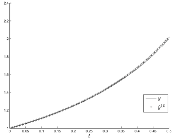
Figure 2: Simulation comparing $y=F_{c}[1]$ to its approximation $\hat{y}^{10}=\hat{F}_{c}^{10}[\Delta]$ in Example 1, case 3.

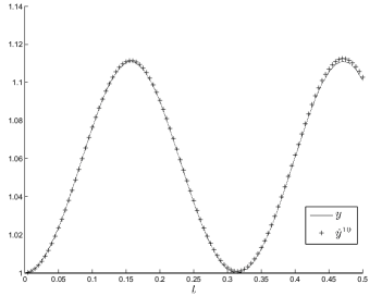
Figure 3: Simulation comparing $y(t)=F_{c}[\sin(20t)]$ to its approximation $\hat{y}^{10}=\hat{F}_{c}^{10}[\hat{u}]$ in Example 1, case 6.

4.3 Globally Convergent $F_{c}$

When $c$ is globally convergent, the divergence problem for $\hat{F}_{c}$ is avoided provided $\hat{u}$ is sufficiently small. But in most cases it is usually not possible to compute the infinite sum defining $\hat{F}_{c}$, so once again the truncated approximator $\hat{F}_{c}^{J}$ will be utilized. The main theorem of this section is given below. It provides an upper bound on the approximation error in terms of the (upper) incomplete gamma function, $\Gamma(a,b):=\int_{b}^{\infty}t^{a-1}{\rm e}^{-t}\,dt/\Gamma(a)$.

Theorem 4.3

Let $c\in\mbox{${\mathbb{R}}^{\ell}_{GC}\langle\langle X\rangle\rangle$}$ with growth constants $K_{c},M_{c}>0$. If $u\in B_{1}^{m}(R)[0,T]$ and $L\gg J$ then

$$\left|F_{c}[u](T)-\hat{F}_{c}^{J}[\hat{u}](L)\right|\lesssim\hat{e}(J)+e(J),\\$$

where

$$\hat{e}(J)=\frac{K_{c}}{2L}{\rm e}^{\hat{s}}\hat{s}^{2}\Gamma(J+1,\hat{s}),\;\;\;e(J)=K_{c}{\rm e}^{s}(1-\Gamma(J+1,s))$$

with $\hat{s}:=M_{c}(m+1)L\|\hat{u}\|_{\infty}$, $s:=M_{c}(m+1)\bar{R}$, and $\bar{R}:=\max\{R,T\}$.

Proof:  Applying Theorem 4.1 gives the following:

$$\left|F_{c}[u](T)-\hat{F}_{c}^{J}[\hat{u}](L)\right| \leq\sum_{j=0}^{J}\sum_{\eta\in X^{j}}\left|(c,\eta)\right|\left|E_{\eta}[u](T,0)-S_{\eta}[\hat{u}](L)\right|+$$

$$\hskip 20.2355pt\sum_{j=J+1}^{\infty}\sum_{\eta\in X^{j}}\left|(c,\eta)\right|\left|E_{\eta}[u](T,0)\right|$$

$$\lesssim\sum_{j=2}^{J}K_{c}M_{c}^{j}(m+1)^{j}\,\frac{T^{j}}{L}\frac{\|\hat{u}/\Delta\|_{\infty}^{j}}{2(j-2)!}+$$

$$\hskip 20.2355pt\sum_{j=J+1}^{\infty}K_{c}M_{c}^{j}(m+1)^{j}\,\frac{\bar{R}^{j}}{j!}$$

$$=\frac{K_{c}}{2L}\sum_{j=0}^{J}(M_{c}(m+1)L\|\hat{u}\|_{\infty})^{j+2}\frac{1}{j!}+$$

$$\hskip 20.2355ptK_{c}\sum_{j=J+1}^{\infty}(M_{c}(m+1)\bar{R})^{j}\frac{1}{j!}$$

$$=\frac{K_{c}}{2L}{\rm e}^{\hat{s}}\hat{s}^{2}\Gamma(J+1,\hat{s})+K_{c}{\rm e}^{s}(1-\Gamma(J+1,s))$$

$$=\hat{e}(J)+e(J),$$

where the identity $\sum_{j=0}^{J}s^{j}/j!={\rm e}^{s}\Gamma(J+1,s)$ has been used (Gradshteyn-Ryzhik_80, , Chapter 8.35).  

Analogous to the local case, the error bound in the previous theorem can be simplified when $L\gg J\gg 1$.

Corollary 2

Let $c\in\mbox{${\mathbb{R}}^{\ell}_{GC}\langle\langle X\rangle\rangle$}$ with growth constants $K_{c},M_{c}>0$. If $u\in B_{1}^{m}(R)[0,T]$ and $L\gg J\gg 1$ then

$$\left|F_{c}[u](T)-\hat{F}_{c}^{J}[\hat{u}](L)\right|\lesssim\frac{K_{c}}{2L}{\rm e}^{M_{c}(m+1)L\|\hat{u}\|_{\infty}}(M_{c}(m+1)L\|\hat{u}\|_{\infty})^{2}.$$

Proof:  The upper bound follows directly from Theorem 4.3 using the fact that $\lim_{J\rightarrow+\infty}$ $\Gamma(J,s)=1$ (since $\Gamma(J+1,s)={\rm e}^{-s}\sum_{j=0}^{J}s^{j}/j!$, $J\geq 0$).  

Example 2

Consider the globally convergent series $c=\sum_{k\geq 0}x_{1}^{k}$ so that $K_{c}=M_{c}=1$. In this case $F_{c}$ has the state space realization

$$\dot{z}=u,\;\;z(0)=0,\;\;y={\rm e}^{z}$$ (7)

since

$$y(t)=\sum_{j=0}^{\infty}(E_{x_{1}}[u](t))^{j}\frac{1}{j!}=\sum_{j=0}^{\infty}E_{x_{1}^{{\scriptscriptstyle\;\sqcup\sqcup\;}j}\frac{1}{j!}}[u](t)=\sum_{j=0}^{\infty}\,E_{x_{1}^{j}}[u](t)=F_{c}[u](t)$$

for all $t\geq 0$. If the constant input $u=1$ is applied over the interval $[0,T]$ then $y(T)={\rm e}^{T}$. The discrete-time approximation at $T=L\Delta$ is

$$\hat{y}^{J}(L) =\hat{F}^{J}_{c}[\Delta](L)=\sum_{j=0}^{J}S_{x_{1}^{j}}[\Delta](L)=\sum_{j=0}^{J}\Delta^{j}\sum_{k_{1}+k_{2}+\cdots+k_{L}=j}1=\sum_{j=0}^{J}\Delta^{j}{L+j-1\choose j}$$

$$=\sum_{j=0}^{J}\frac{\Delta^{j}}{j!}\left(L^{j}+\frac{(j-1)j}{2}L^{j-1}+\cdots+(j-1)!L\right)$$

$$\approx\sum_{j=0}^{J}\frac{T^{j}}{j!}+\frac{1}{2L}\sum_{j=2}^{J}\frac{T^{j}}{(j-2)!}$$

$$=[F_{c}[1](T)-e(J)]+\hat{e}(J),$$

which is consistent with Theorem 4.3 and again the worst case scenario in terms of approximating the iterated integrals. The outputs $y$ and $\hat{y}$ were computed numerically over the interval $[0,2]$ for various choices of $u$, $L$, and $J$. This data is summarized in Table 3, and the corresponding plots for cases 3 and 6 are shown in Figures 4 and 5, respectively. As in the previous example, most of the error in the approximation is due to the term $\hat{e}(J)$, and the constant input case yields an error that is approximately upper bounded by $\hat{e}(J)+e(J)$. The error bound for the sinusoidal input is again conservative.

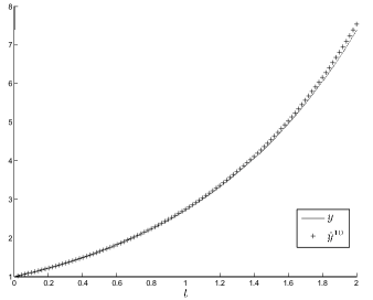
Figure 4: Simulation comparing $y=F_{c}[1]$ to its approximation $\hat{y}^{10}=\hat{F}_{c}^{10}[\Delta]$ in Example 2, case 3.

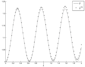
Figure 5: Simulation comparing $y(t)=F_{c}[\sin(10t)]$ to its approximation $\hat{y}^{10}=\hat{F}_{c}^{10}[\hat{u}]$ in Example 2, case 6.

5 Approximating Rational Operators

In the case where $F_{c}$ is a rational operator, it is shown in this section that the approximation $\hat{F}_{c}$ can be computed without the need for truncation. This is due exclusively to the fact that the generating series for such an operator has structure which is not available in general, namely, a linear representation as described in Definition 2. The main idea is to use this representation to construct a discrete-time state space realization for $\hat{F}_{c}$. Later it will be shown that this technique is directly related to a specific discretization of the corresponding bilinear state space realization of $F_{c}$. But the connection only becomes apparent in retrospect. For simplicity, the focus will be on the single-output case. As motivation, consider the following simple example.

Example 3

If $c=x_{i_{3}}x_{i_{2}}x_{i_{1}}\in X^{\ast}$ then the corresponding discrete-time Fliess operator is $\hat{y}=S_{x_{i_{3}}x_{i_{2}}x_{i_{1}}}[\hat{u}]$. Define the state $\hat{z}_{1}=S_{x_{i_{1}}}[\hat{u}]$ so that

$$\hat{z}_{1}(N+1)=\hat{z}_{1}(N)+\hat{u}_{i_{1}}(N+1).$$

Similarly, if $\hat{z}_{2}=S_{x_{i_{2}i_{1}}}[\hat{u}]$ then

$$\hat{z}_{2}(N+1) =\hat{z}_{2}(N)+\hat{u}_{i_{2}}(N+1)\hat{z}_{1}(N+1)$$

$$=\hat{z}_{2}(N)+\hat{z}_{1}(N)\hat{u}_{i_{2}}(N+1)+\hat{u}_{i_{2}}(N+1)\hat{u}_{i_{1}}(N+1).$$

Finally, setting $\hat{y}=\hat{z}_{3}=S_{x_{i_{3}}x_{i_{2}}x_{i_{1}}}[\hat{u}]$ gives

$$\hat{z}_{3}(N+1) =\hat{z}_{3}(N)+\hat{z}_{2}(N)\hat{u}_{i_{3}}(N+1)+\hat{z}_{1}(N)\hat{u}_{i_{3}}(N+1)\hat{u}_{i_{2}}(N+1)+$$

$$\hskip 20.2355pt\hat{u}_{i_{3}}(N+1)\hat{u}_{i_{2}}(N+1)\hat{u}_{i_{1}}(N+1).$$

This triangular polynomial system is clearly not input-affine, as would be the case for the analogous continuous-time input-output system $y=E_{x_{i_{3}}x_{i_{2}}x_{i_{1}}}[u]$, but the realization is state affine in the following sense.

Definition 6

A discrete-time state space realization is polynomial input and state affine if its transition map has the form

$$\hat{z}_{i}(N+1)=\sum_{j=1}^{n}p_{ij}(\hat{u}(N+1))\hat{z}_{j}(N)+q_{i}(\hat{u}(N+1)),$$

$i=1,2,\ldots,n$, where $\hat{z}(N)\in\mathbb{R}^{n}$, $\hat{u}=[\hat{u}_{0},\hat{u}_{1},\ldots,\hat{u}_{m}]^{T}$, $p_{ij}$ and $q_{i}$ are polynomials, and the output map $h:\hat{z}\mapsto\hat{y}$ is linear.

Polynomial input, state affine systems constitute an important class of discrete-time systems as first observed by Sontag in (Sontag_79, , Chapter V). The fact that $\hat{u}(N+1)$ appears in the transition map instead of $\hat{u}(N)$, as is more common, has no serious consequences here. It will turn out, however, that if $c$ is rational instead of being merely polynomial, a more general class of state space realization is required, one where rational functions of the input are admissible.

Definition 7

A discrete-time state space realization is rational input and state affine if its transition map has the form

$$\hat{z}_{i}(N+1)=\sum_{j=1}^{n}r_{ij}(\hat{u}(N+1))\hat{z}_{j}(N)+s_{i}(\hat{u}(N+1)),$$

$i=1,2,\ldots,n$, where $\hat{z}(N)\in\mathbb{R}^{n}$, $\hat{u}=[\hat{u}_{0},\hat{u}_{1},\ldots,\hat{u}_{m}]^{T}$, $r_{ij}$ and $s_{i}$ are rational functions, and the output map $h:\hat{z}\mapsto\hat{y}$ is linear.

The main theorem of the section is below.

Theorem 5.1

Let $c\in\mathbb{R}\langle\langle X\rangle\rangle$ be a rational series over $X=\{x_{0},x_{1},\ldots,x_{m}\}$ with representation $(\mu,\gamma,\lambda)$. Then $\hat{y}=\hat{F}_{c}[\hat{u}]$ has a finite dimensional rational input and state affine realization on $B_{\infty}^{m+1}[0,N_{f}](\hat{R})$ for any $N_{f}>0$ provided $\hat{R}>0$ is sufficiently small.

Before giving the proof, some preliminary results are needed.

Lemma 4

For any $c\in\mbox{${\mathbb{R}}\langle\langle X\rangle\rangle$}$ it follows that

$$\hat{F}_{c}[\hat{u}](N+1)=\hat{F}_{c}[\hat{u}](N)+\sum_{j=0}^{m}\hat{u}_{j}(N+1)\,\hat{F}_{x_{j}^{-1}(c)}[\hat{u}](N+1).$$

Proof: Observe that

$$\hat{F}_{c}[\hat{u}](N+1) =\sum_{\eta\in X^{\ast}}(c,\eta)S_{\eta}[\hat{u}](N+1)$$

$$=\sum_{j=0}^{m}\sum_{\eta\in X^{\ast}}(c,x_{j}\eta)\sum_{k=0}^{N+1}\hat{u}_{j}(k)S_{\eta}[\hat{u}](k)$$

$$=\sum_{j=0}^{m}\sum_{\eta\in X^{\ast}}(c,x_{j}\eta)\left[\sum_{k=0}^{N}\hat{u}_{j}(k)S_{\eta}[\hat{u}](k)+\hat{u}_{j}(N+1)S_{\eta}[\hat{u}](N+1)\right]$$

$$=\hat{F}_{c}[\hat{u}](N)+\sum_{j=0}^{m}\hat{u}_{j}(N+1)\sum_{\eta\in X^{\ast}}(x_{j}^{-1}(c),\eta)S_{\eta}[\hat{u}](N+1)$$

$$=\hat{F}_{c}[\hat{u}](N)+\sum_{j=0}^{m}\hat{u}_{j}(N+1)\hat{F}_{x_{j}^{-1}(c)}[\hat{u}](N+1).$$

 

The next theorem hints at the well known dichotomy between time-reversible and non-time-reversible discrete-time systems. That is, while every continuous-time state space realization can be run in reverse time, this is definitely not the case for discrete-time systems. The system in the following theorem will only be time-reversible under certain conditions.

Theorem 5.2

Let $c\in\mathbb{R}\langle\langle X\rangle\rangle$ be a rational series over $X=\{x_{0},x_{1},\ldots,x_{m}\}$. Then $\hat{y}=\hat{F}_{c}[\hat{u}]$ has a finite dimensional backward-in-time bilinear realization for any input sequence $\hat{u}$ defined over $[0,N_{f}]$.

Proof: Since $c$ is rational, it follows from Theorem 2.2 that a stable $n$ dimension subspace $V$ of ${\mathbb{R}}\langle\langle X\rangle\rangle$ exists which contains $c$. Let $\bar{c}_{k}$, $k=1,2,\ldots,n$ be a basis for $V$ so that $c=\sum_{k=1}^{n}\lambda_{k}\bar{c}_{k}$ with $\lambda_{k}\in{\mathbb{R}}$. Furthermore, for any $x_{j}\in X$ it follows that

$$x_{j}^{-1}(\bar{c}_{k})=\sum_{l=1}^{n}\mu_{kl}(x_{j})\,\bar{c}_{l},$$

where $\mu_{kl}(x_{j})\in{\mathbb{R}}$. Define the state variables $\bar{z}_{k}(N)=\hat{F}_{\bar{c}_{k}}[\hat{u}](N_{f}-N)$, $k=1,2,\ldots,n$ for $N\in[0,N_{f}]$. Then

$$\hat{y}(N)=\hat{F}_{c}[\hat{u}](N)=\sum_{k=1}^{n}\lambda_{k}\hat{F}_{\bar{c}_{k}}[\hat{u}](N)=\sum_{k=1}^{n}\lambda_{k}\bar{z}_{k}(N_{f}-N)$$

and

$$\bar{z}_{k}(N_{f})=\hat{F}_{\bar{c}_{k}}[\hat{u}](0)=(\bar{c}_{k},\emptyset)S_{\emptyset}[\hat{u}](0)=(\bar{c}_{k},\emptyset)=:\gamma_{k}.$$

Now from Lemma 4

$$\bar{z}_{k}(N_{f}-N-1) =\bar{z}_{k}(N_{f}-N)\!+\!\sum_{j=0}^{m}\hat{u}_{j}(N+1)\,\hat{F}_{x_{j}^{-1}(\bar{c}_{k})}[\hat{u}](N+1)$$

$$=\bar{z}_{k}(N_{f}-N)\!+\!\sum_{j=0}^{m}\hat{u}_{j}(N+1)\sum_{l=1}^{n}\mu_{kl}(x_{j})\hat{F}_{\bar{c}_{l}}[\hat{u}](N+1)$$

$$=\bar{z}_{k}(N_{f}-N)\!+\!\sum_{j=0}^{m}\hat{u}_{j}(N+1)\sum_{l=1}^{n}\mu_{kl}(x_{j})\bar{z}_{l}(N_{f}-N-1)$$

$$=\bar{z}_{k}(N_{f}-N)\!+\!\sum_{j=0}^{m}\hat{u}_{j}(N+1)\,[A_{j}\bar{z}(N_{f}-N-1)]_{k},$$

where $A_{j}\in{\mathbb{R}}^{n\times n}$, $j=0,1,\ldots,m$ has components $[A_{j}]_{kl}=\mu_{kl}(x_{j})$, and $\bar{z}$ is the column vector with $\bar{z}_{k}$ as its $k$-th component. Therefore, for $N=N_{f}-1,N_{f}-2,\ldots,0$ it follows that

$$\bar{z}(N_{f}-N)=\left[I-\sum_{j=0}^{m}A_{j}\hat{u}_{j}(N+1)\right]\bar{z}(N_{f}-N-1),$$

with $\bar{z}(N_{f})=\gamma$ and $\hat{y}(N)=\lambda\bar{z}(N_{f}-N)$, or equivalently, setting $\hat{z}(N)=\bar{z}(N_{f}-N)$ gives for $N=N_{f}-1,N_{f}-2,\ldots,0$

$$\hat{z}(N)=\left[I-\sum_{j=0}^{m}A_{j}\hat{u}_{j}(N+1)\right]\hat{z}(N+1)$$ (8)

with $\hat{z}(0)=\gamma$ and $\hat{y}(N)=\lambda\hat{z}(N)$ as claimed.  

The proof of the main result follows from introducing conditions on $\hat{u}$ so that system (8) is time-reversible. Bilinearity is lost in the process, but the forward-in-time system is rational input and state affine.

Proof of Theorem 5.1: If $\hat{u}\in B_{\infty}^{m+1}[0,N_{f}](\hat{R})$, and $\hat{R}$ is sufficiently small, then the transition matrix $I-\sum_{j=0}^{m}A_{j}\hat{u}_{j}(N+1)$ of system (8) is nonsingular. In which case, the forward-in-time system

$$\hat{z}(N+1)=\left[I-\sum_{j=0}^{m}A_{j}\hat{u}_{j}(N+1)\right]^{-1}\hat{z}(N)$$

is well defined over $[0,N_{f}]$ and clearly state affine and rational in $\hat{u}$. Furthermore, by design $\hat{y}=F_{c}[\hat{u}]=\lambda\hat{z}$ over the interval $[0,N_{f}]$.  

Example 4

Reconsider the rational Fliess operator in Example 2 where $c=\sum_{k\geq 0}x_{1}^{k}$. Clearly, $x_{0}^{-1}(c)=0$, $x_{1}^{-1}(c)=c$, and $(c,\emptyset)=1=1\cdot 1=\lambda\gamma$. Thus, $\hat{F}_{c}$ has the $n=1$ dimensional rational and state affine realization

$$\hat{z}(N+1)=(1-\hat{u}(N+1))^{-1}\hat{z}(N),\;\;\hat{z}(0)=1,\;\;\hat{y}(N)=\hat{z}(N)$$ (9)

provided $\|\hat{u}\|_{\infty}<1$. Since

$$\hat{z}(N+1)=\sum_{i=0}^{\infty}\hat{u}^{i}(N+1)\hat{z}(N),$$

if follows for $N\geq 0$ that

$$\hat{y}(N)=\prod_{k=1}^{N}(1-\hat{u}(k))^{-1}\hat{z}(0)=\sum_{i_{1},\ldots,i_{N}=0}^{\infty}\hat{u}^{i_{N}}(N)\hat{u}^{i_{N-1}}(N-1)\cdots\hat{u}^{i_{1}}(1),$$

where the product is defined to be unity when $N=0$. For example,

$$\hat{y}(0) =1$$

$$\hat{y}(1) =1+\hat{u}(1)+\hat{u}^{2}(1)+\hat{u}^{3}(1)+\cdots$$

$$\hat{y}(2) =(1+\hat{u}(2)+\hat{u}^{2}(2)+\cdots)(1+\hat{u}(1)+\hat{u}^{2}(1)+\cdots)$$

$$=1+(\hat{u}(1)+\hat{u}(2))+(\hat{u}^{2}(1)+\hat{u}(2)\hat{u}(1)+\hat{u}^{2}(2))+$$

$$\hskip 14.45377pt(\hat{u}^{3}(1)+\hat{u}^{2}(2)\hat{u}(1)+\hat{u}(2)\hat{u}^{2}(1)+\hat{u}^{3}(2))+\cdots$$

$$\hskip 7.22743pt\vdots$$

This solution can be checked independently by simply applying the definition of $\hat{F}_{c}$. That is,

$$\hat{y}(N)=S_{\emptyset}[\hat{u}](N)+S_{x_{1}}[\hat{u}](N)+S_{x_{1}^{2}}[\hat{u}](N)+\cdots,$$

so that

$$\hat{y}(0) =1$$

$$\hat{y}(1) =1+\hat{u}(1)+\hat{u}^{2}(1)+\hat{u}^{3}(1)+\cdots$$

$$\hat{y}(2) =1+(\hat{u}(1)+\hat{u}(2))+(\hat{u}^{2}(1)+\hat{u}(2)\hat{u}(1)+\hat{u}^{2}(2))+$$

$$\hskip 14.45377pt(\hat{u}^{3}(1)+\hat{u}^{2}(2)\hat{u}(1)+\hat{u}(2)\hat{u}^{2}(1)+\hat{u}^{3}(2))+\cdots$$

$$\hskip 7.22743pt\vdots$$

Not surprisingly, the plots of $\hat{y}$ generated from system (9) are indistinguishable from those shown in Figures 4 and 5, which were generated directly from the definition of $\hat{F}_{c}^{J}$. It also should be noted that $F_{c}$, being rational, has a bilinear realization

$$\dot{\tilde{z}}=\tilde{z}u,\;\;\tilde{z}(0)=1,\;\;y=\tilde{z},$$

which is related to the realization (7) by the coordinate transformation $\tilde{z}={\rm e}^{z}$. For small $\Delta>0$ observe

$$\tilde{z}((N+1)\Delta) =\tilde{z}(N\Delta)+\int_{N\Delta}^{(N+1)\Delta}\tilde{z}(t)u(t)\,dt$$

$$\approx\tilde{z}(N\Delta)+\int_{N\Delta}^{(N+1)\Delta}u(t)\,dt\,\,\tilde{z}((N+1)\Delta)$$

$$=\tilde{z}(N\Delta)+\hat{u}(N+1)\,\tilde{z}((N+1)\Delta),$$

and therefore, letting $\hat{z}(N)=\tilde{z}(N\Delta)$, this particular discretized system

$$\hat{z}(N+1)=(1-\hat{u}(N+1))^{-1}\hat{z}(N)$$

has the form of (9).

Example 5

The previous example can be generalized by noting that

$$\hat{z}(N+1) =\left[I-\sum_{j=0}^{m}A_{j}\hat{u}_{j}(N+1)\right]^{-1}\hat{z}(N)$$

$$=\left[\sum_{k=0}^{\infty}\sum_{j_{0},\ldots,j_{k}=0}^{m}A_{j_{0}}A_{j_{1}}\cdots A_{j_{k}}\hat{u}_{j_{0}}(N+1)\hat{u}_{j_{1}}(N+1)\cdots\hat{u}_{j_{k}}(N+1)\right]\hat{z}(N)$$

$$=:\sum_{\eta=x_{j_{0}}\cdots x_{j_{k}}\in X^{\ast}}A_{\eta}\hat{u}_{\eta}(N+1)\hat{z}(N).$$

In which case,

$$\hat{y}(N) =\sum_{\eta_{N},\ldots,\eta_{1}\in X^{\ast}}\lambda A_{\eta_{N}}\cdots A_{\eta_{1}}\gamma\;\hat{u}_{\eta_{N}}(N+1)\cdots\hat{u}_{\eta_{1}}(1)$$

$$=\sum_{\eta_{N},\ldots,\eta_{1}\in X^{\ast}}(c,\eta_{N}\cdots\eta_{1})\hat{u}_{\eta_{N}}(N+1)\cdots\hat{u}_{\eta_{1}}(1).$$

This form of the discrete-time input-output map comes from a specific discretization of the underlying continuous-time realization

$$\dot{z}(t)=\sum_{j=0}^{m}A_{j}z(t)u_{j},\;\;z(0)=\gamma,\;\;y(t)=\lambda z(t),$$

namely,

$$z((N+1)\Delta)\approx z(N\Delta)+\sum_{j=0}^{m}A_{j}\hat{u}_{j}(N+1)\,z((N+1)\Delta)$$

so that

$$\hat{z}(N+1)=\left[I-\sum_{j=0}^{m}A_{j}\hat{u}_{j}(N+1)\right]^{-1}\hat{z}(N).$$

6 Conclusions

This paper described how to approximate Fliess operators with iterated sums and gave explicit achievable error bounds for the locally and globally convergent cases. For the special case of rational Fliess operators, it was shown that the method can be realized via a rational input and state affine discrete-time state space model. This model avoids the truncation error and can also be derived from a specific discretization of a continuous-time bilinear realization of the rational Fliess operator.

Table 2: Summary of simulation results for Example 1.

case	$u$	$T$	$L$	$\Delta$	$J$	$\|\hat{u}\|_{\infty}$	$s$	$\hat{s}$	$y(T)$	$\hat{y}^{J}(L)$	$\hat{y}^{J}(L)-y(T)$	$\hat{e}(J)$	$e(J)$
1	$1$	0.5	50	0.0100	10	0.0100	0.5000	0.5000	2.0000	2.0412	0.0412	0.0355	9.7656$\times 10^{-4}$
2	$1$	0.5	50	0.0100	20	0.0100	0.5000	0.5000	2.0000	2.0448	0.0448	0.0400	9.5367$\times 10^{-7}$
3	$1$	0.5	100	0.0050	10	0.0050	0.5000	0.5000	2.0000	2.0192	0.0192	0.0177	9.7656$\times 10^{-4}$
4	$\sin(20t)$	0.5	50	0.0100	10	0.0099	0.5000	0.4975	1.1009	1.1041	0.0032	0.0347	9.7656$\times 10^{-4}$
5	$\sin(20t)$	0.5	50	0.0100	20	0.0099	0.5000	0.4975	1.1009	1.1041	0.0032	0.0390	9.5367$\times 10^{-7}$
6	$\sin(20t)$	0.5	100	0.0050	10	0.0050	0.5000	0.4994	1.1011	1.1028	0.0017	0.0176	9.7656$\times 10^{-4}$

Table 3: Summary of simulation results for Example 2.

case	$u$	$T$	$L$	$\Delta$	$J$	$\|\hat{u}\|_{\infty}$	$s$	$\hat{s}$	$y(T)$	$\hat{y}^{J}(L)$	$\hat{y}^{J}(L)-y(T)$	$\hat{e}(J)$	$e(J)$
1	$1$	2	50	0.0400	10	0.0400	2.0000	2.0000	7.3891	7.6989	0.3098	0.2956	6.1390$\times 10^{-5}$
2	$1$	2	50	0.0400	20	0.0400	2.0000	2.0000	7.3891	7.6991	0.3100	0.2956	4.5119$\times 10^{-14}$
3	$1$	2	100	0.0200	10	0.0200	2.0000	2.0000	7.3891	7.5403	0.1512	0.1478	6.1390$\times 10^{-5}$
4	$\sin(10t)$	2	50	0.0400	10	0.0392	2.0000	1.9601	1.0601	1.0803	0.0202	0.2728	6.1390$\times 10^{-5}$
5	$\sin(10t)$	2	50	0.0400	20	0.0392	2.0000	1.9601	1.0601	1.0803	0.0202	0.2728	4.5119$\times 10^{-14}$
6	$\sin(10t)$	2	100	0.0200	10	0.0199	2.0000	1.9899	1.0607	1.0711	0.0104	0.1448	6.1390$\times 10^{-5}$

References

- (1) J. Berstel and C. Reutenauer, Rational Series and Their Languages, Springer-Verlag, Berlin, 1988.
- (2) S. Butler and P. Karasik, A note on nested sums, J. Integer Seq., 13 (2010) article 10.4.4.
- (3) K.-T. Chen, Iterated integrals and exponential homomorphisms, Proc. Lond. Math. Soc., 4 (1954) 502–512.
- (4) M. Fliess, Fonctionnelles causales non linéaires et indéterminées non commutatives, Bull. Soc. Math. France, 109 (1981) 3–40.
- (5) , Réalisation locale des systèmes non linéaires, algèbres de Lie filtrées transitives et séries génératrices non commutatives, Invent. Math., 71 (1983) 521–537.
- (6) I. S. Gradshteyn and I. M. Ryzhik, Tables of Integrals, Series, and Products, 4th Ed., Academic Press, Orlando, FL, 1980.
- (7) W. S. Gray, L. A. Duffaut Espinosa, K. Ebrahimi-Fard, Faà di Bruno Hopf algebra of the output feedback group for multivariable Fliess operators, Systems Control Lett., 74 (2014) 64–73.
- (8) , Analytic left inversion of multivariable Lotka-Volterra models, Proc. 54nd IEEE Conf. on Decision and Control, Osaka, Japan, 2015, to appear.
- (9) W. S. Gray, L. A. Duffaut Espinosa, and M. Thitsa, Left inversion of analytic nonlinear SISO systems via formal power series methods, Automatica, 50 (2014) 2381–2388.
- (10) W. S. Gray and Y. Li, Generating series for interconnected analytic nonlinear systems, SIAM J. Control Optim., 44 (2005) 646–672.
- (11) W. S. Gray and Y. Wang, Fliess operators on spaces: convergence and continuity, Systems Control Lett., 46 (2002) 67–74.
- (12) L. Grüne and P. E. Kloeden, Higher order numerical schemes for affinely controlled nonlinear systems, Numer. Math., 89 (2001) 669–690.
- (13) F. He, P. Zhang, Y. Chen, L. Wang, Y. Yao, and W. Chen, Output tracking control of switched hybrid systems: A Fliess functional expansion approach, Math. Probl. Eng., 2013 (2013) article 412509.
- (14) A. Isidori, Nonlinear Control Systems, 3rd Ed., Springer-Verlag, London, 1995.
- (15) E. D. Sontag, Polynomial Response Maps, Springer-Verlag, Berlin, 1979.
- (16) Y. Yao, B. Yang, F. He, Y. Qiao, and D. Cheng, Attitude control of missile via Fliess expansion, IEEE Trans. Control Syst. Technol., 16 (2008) 959–970.