Interaction between catalytic micro motors

Abstract

Starting from a microscopic model for a spherically symmetric active Janus particle, we study the interactions between two such active motors. The ambient fluid mediates a long range hydrodynamic interaction between two motors. This interaction has both direct and indirect hydrodynamic contributions. The direct contribution is due to the propagation of fluid flow that originated from a moving motor and affects the motion of the other motor. The indirect contribution emerges from the re-distribution of the ionic concentrations in the presence of both motors. Electric force exerted on the fluid from this ionic solution enhances the flow pattern and subsequently changes the motion of both motors. By formulating a perturbation method for very far separated motors, we derive analytic results for the transnational and rotational dynamics of the motors. We show that the overall interaction at the leading order, modifies the translational and rotational speeds of motors which scale as ${\cal O}\left([1/D]^{3}\right)$ and ${\cal O}\left([1/D]^{4}\right)$ with their separation, respectively. Our findings open up the way for studying the collective dynamics of synthetic micro motors.

I Introduction

Designing the synthetic micro propelling systems with ability to navigate in predefined and controllable trajectories are the aim of many researchers both in chemistry and physics.molmach Delivery of drug at living systems and construction of manipulating tools for lab on chip experiments are among the main applications of such systems. Hydrodynamic swimmers,laugareview ; rojman2s ; 2s single DNA molecule propeller,dna light mediated motion of Janus particles in binary mixtures and colloidal systemsbuttinoni ; palacci and phoretic propulsion of spheroidal particlespopescu are most recent proposed designs for micro machines.

Apart from their potential applications as listed above, the physics of directed motion at the scale of micrometer is also a challenging issue in physics.brady0 ; julichercomment This is mainly due to the inertia-less condition that constrains the physics at this scale. At macroscopic scale of the daily life, inertia provides a mechanism for movements, but at microscopic scale, the life is dominated by dissipation. As a result of this ambiguity, a backward ejection of a high-speed jet of molecules is not able to propel a micron size boat. For driving a micrometer boat, we need to go beyond our macroscopic feeling of motion and use nontrivial mechanisms for swimming strategies.purcell1977life ; laugareview ; 3s

Janus particles with surface chemical activity are potential proposals for cargo delivery machines at the scale of micrometer. Originated from a very interesting experiment by Paxton, et. al.,paxton1 ; paxton2 a great deal of the researcher’s attention has been attracted by the idea of generating directed motion by surface reactions.howse ; wang1 ; wang2 ; brown As a recent example, Janus particles made from spherical Pt insulator have been studied extensively.ebbens1 ; ebbens2 Drug delivery baraban ; sundararajan ; patra ; wu ; kagan2 ; mou and ability for entering into cells by catalytic Janus particles gao have been examined experimentally. Another interesting application of catalytic micro-motors includes water purification that, has been successfully tested.soler ; wang4 Also it is shown that using Janus particles, one can make a chemical sensor.kagan1 Understanding and predicting the physical behavior of a single or many such motors constitute the core of many recent researches.walther

The physics of a single Janus particle propeller has been investigated theoretically luga1 and numerically.moran ; daghighi ; sharifi1 Recently, motion of Janus self propellers in different conditions have been considered. This include dynamic of a particle confined by a planar wall and also motion in shear flow. It is shown that depending on the initial state of a Janus particle, a rigid and electrically neutral wall can both attract or repel a nearby Janus motor.uspal ; crowdy The dynamical response of a Janus motor moving in an ambient shear flow have a crucial dependence on the strength of thermal fluctuations of the ions.khair

For most of the expected applications of micro machines, it is reasonable to use a collection of them to achieve maximum efficiency. Along this task, one need to have an understanding of the physics of mutual interaction between two or many of Janus motors. Such theoretical knowledge will allow the researchers to predict the collective behavior of a suspension of many Janus motors system. So far and up to our knowledge, all theoretical works are limited to the physics of individual motors. In this article we address the problem of interaction between two self propelled Janus motors.

A number of interesting phenomena in a system of two or many hydrodynamical swimmers have been observed. These includes a class of phenomena ranging from coherent motion of two coupled swimmers najafi2010coherent ; farzin2012general ; pooley2007hydrodynamic to pattern formation and reduction of effective viscosity in suspensions.childress1975pattern ; dombrowski2004self ; baskaran2009statistical ; hatwalne2004rheology ; moradi2015rheological Inspiring from these hydrodynamical systems, we expect to see a rich physical behavior in the case of Janus particles those are electro-hydrodynamical and in addition to hydrodynamic effects, the presence of long range electrostatic forces should also be considered.

The rest of this article organizes as follow: In section II we introduce the system and write the basic governing equations. Sections III and IV are devoted to develop the approximations that we will use. Analytic results for a single motor are collected in section V and the problem of interacting particles is presented in section VI. Finally, discussion about our results is presented in section VII.

II Governing equations

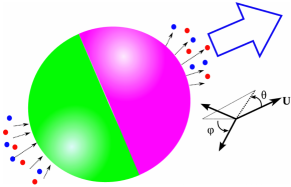
Figure 1: A spherical micron size particle benefits surface reactions to propel itself. Surface activity of the particle, allow both production and absorption of ionic molecules. With respect to a co-moving reference frame, an azimuthally symmetric but polar pattern of surface activity, is able to produce a net propulsion.

We start by analyzing the physics of a single motor that, benefits surface chemical reactions to propel itself. A schematic view of the model system that we are interested to analyze, is shown in Figure 1. A charged colloidal particle with radius $a$ and electrostatic surface potential given by $\psi_{s}$, is immersed in an electrolyte solution with electric permeability $\varepsilon_{r}$ and hydrodynamic viscosity $\eta$. Solution consists of two ionic species, cations and anions with valances given by $Z_{\pm}$, respectively (throughout this paper, $+$ refers to cations and $-$ refers to anions). We consider the simple case where the electrolyte is symmetric and single valence with $Z_{+}=-Z_{-}=1$. Driving force of this motor emerges from an asymmetric surface chemical activity. We assume that the surface properties of the motor, allows it to absorb and emit chemical species in an asymmetric way. As shown in figure, the north hemisphere of the Janus particle can emit ionic particles, either cations and anions. The south hemisphere of the Janus particle can absorb the ions with the same rate given at the emitting part. Such a simple modeling can take into account the physics of most experimentally realized Janus motors.

We use dimensionless units to introduce the dynamical equations. In addition to simplifying the notations, dimensionless form of the equations will help us to introduce our approximate scheme for solving the equations. We will use the radius of the motor $a$, potential associated with thermal energy $\psi_{0}=(k_{B}T/e)$ and equilibrium concentration of ions at infinity $n_{\infty}$, to make non dimensional form for all length scales, electric potential and concentrations, respectively. A velocity scale given by $v_{0}=(k_{B}T/e)^{2}(\varepsilon_{r}/\eta a)$ and a characteristic pressure $p_{0}=v_{0}\eta/a$ will be used to make the velocities and pressures non dimensional.

Denoting the ionic fluxes of cations and anions by ${\bf j}_{\pm}({\bf x})$, we consider a prescribed surface activity given by the following condition on the fluxes:

$${\bf\hat{n}}\cdot{\bf j}_{\pm}({\bf r}={\hat{\bf n}})={\dot{Q}}\cos\theta,$$ (1)

where ${\bf j}_{\pm}({\hat{\bf n}})={\bf j}_{\pm}^{s}$, shows the current densities given on the surface of the spherical Janus particle. In the above equation, ${\dot{Q}}$ is a constant ionic rate, $\theta$ is the azimuthal angle with respect to a fixed $z-$axes co-moving with the motor and ${\bf\hat{n}}$ represents a unit vector that is normal to the surface. For the above model of surface activity, total number of both ionic species in the solution are fixed. In addition to the catalytic realization of our model, it can also be considered as a motor that works base on an osmotic pressure difference. One can consider a sphere that is constructed by a semi-permeable membrane. An internal active compartment inside the motor, provides an angle dependent osmotic pressure difference between inside and outside of the motor. Due to this pressure difference, the above surface ionic flow can appear in the system.

As a result of this asymmetric surface property, the motor will achieve a constant steady state propulsion velocity. We would like to calculate this propulsion velocity as a function of the physical properties of the motor and the electrolyte characteristics.

Simultaneous solution to the hydrodynamic equations and the electrostatic equations for the ionic concentrations, will reveal the propulsion velocity. These two sets of equations are coupled via the hydrodynamic body force that appears in the hydrodynamic equations. As discussed before, the hydrodynamics of a micron scale system should be described by governing equations at very small inertia condition. Neglecting the inertial effects, the Stokes equation governs the dynamics of the fluid at fully dissipative limit:landau1987fluid

$$\nabla^{2}{\bf u}({\bf r})-\nabla p({\bf r})=-(n_{+}({\bf r})-n_{-}({\bf r}))\nabla\psi({\bf r}),$$ (2)

where ${\bf u}({\bf r})$ and $P({\bf r})$ stand for velocity and pressure field of the fluid. Assuming that the fluid is in-compressible, the velocity field should satisfy a continuity equation as: $\nabla\cdot\ {\bf u}({\bf r})=0$. Right hand side of the Stokes equation represents an electric body force acting on the fluid that comes from the ions, where $n_{\pm}({\bf r})$ and $\psi({\bf r})$ are ionic concentrations and electric potential of the ions. The electrostatic potential satisfies the Poisson-Boltzmann equation:

$$\delta^{2}\nabla^{2}\psi=-\frac{1}{2}(n_{+}-n_{-}).$$ (3)

Continuity equations for the ionic currents are another equations that should be satisfied. The continuity equations for ions read:

$$\frac{\partial n_{\pm}({\bf r})}{\partial t}+\nabla\cdot{\bf j}_{\pm}({\bf r})=0.$$ (4)

Thermal fluctuations of the ions, drift due to the electric forces and convection due to the flow of fluid are different sources for the ionic currents. Collecting all these terms, we can write the following phenomenological relations for the ionic currents as:

$${\bf j}_{\pm}({\bf r})=-\nabla n_{\pm}({\bf r})\ \mp n_{\pm}({\bf r})\nabla\psi({\bf r})+{\cal P}en_{\pm}({\bf r}){\bf u}({\bf r}).$$ (5)

where the phenomenological contribution from the fluctuations is expressed in terms of the concentration gradient.

Two important dimensionless numbers, $\delta$ and ${\cal P}e$ that are appeared in governing equations, are given by:

$$\delta^{2}=1/(\kappa a)^{2}=\frac{\varepsilon_{r}k_{B}T}{2e^{2}n_{\infty}a^{2}},~{}~{}{\cal P}e=\frac{\varepsilon_{r}(k_{B}T)^{2}}{\eta e^{2}D}.$$ (6)

Debye screening length $\delta$, measures the equilibrium thickness of ionic cloud around a colloid which is immersed in an ionic solution. This is essentially a length beyond which the electric effects of the colloid screened. Peclet number ${\cal P}e$, measures how the convection is effective in comparison with thermal diffusion. For very small Peclet number, the current due to the thermal fluctuations is dominated over the current from convection. In our description of the system, and for mathematical simplifications, the diffusion constants for both ions are assumed to be equal and we denote both of them by $D$. In general the ionic diffusion constants depend on the size of ions, that result a different values for cations and anions. As we are not interested about the phenomena that could result from such asymmetry between cations and anions, we restrict ourselves to the symmetric case with equal diffusion constants.

In addition to the boundary condition given by equation 1, there are other boundary conditions that should be considered. On the surface of motor and in a co-moving frame, the boundary conditions for the fluid velocity and ionic potential read:

$${\bf u}({\bf r})=0,~{}~{}~{}~{}\psi({\bf r})=\psi_{s},~{}~{}~{}~{}~{}~{}{\bf r}=a\hat{{\bf n}}.$$

Very far from the motor, at $r\rightarrow\infty$, the boundary conditions read:

$${\bf u}({\bf r})=-{\bf U},~{}~{}~{}\nabla\psi({\bf r})=0,~{}~{}~{}~{}\psi({\bf r})=0,~{}~{}~{}~{}n_{\pm}=n_{\infty},$$

where ${\bf U}$, is the propulsion velocity of the motor, that needs to be determined by solving the above equations. As the motor propulsion is not due to any external force, total force acting on the motor vanishes. Collecting both the hydrodynamic and electrostatic forces acting on the spherical motor, the force free condition can be written as:

$${\bf F}=\oint_{S} \left\{-p\mathbb{I}+\nabla{\bf u}+(\nabla{\bf u})^{T}\right.$$ (7)

$$\left.+\nabla\psi\nabla\psi-\frac{1}{2}\nabla\psi\cdot\nabla\psi\mathbb{I}\right\}\cdot{\bf\hat{n}}\ dS=0,$$

where $\mathbb{I}$ refers to the $3\times 3$ unit matrix, and superscript $T$ refers to transpose of a square matrix.

For a typical experiment that we are interested, A micron sized particle with $a\sim 1\mu m$, moves in an electrolyte solution with $\eta\sim 10^{-3}\text{Pa~{}sec}$, $D=\times 10^{-9}\text{m}^{2}/\text{sec}$ and $n_{\infty}=10^{23}m^{-3}$ (data are given for $0.001$ molar solution of $KCL$ at room temperature).ohshima2006theory In this case, we will have $\delta\sim 10^{-3}$ and ${\cal P}e\sim 10^{-1}$. For a typical system with these numerical values for physical parameters, we can proceed by applying the condition $\delta\ll 1$ to the dynamical equations and obtain approximate analytic results. In the limit of strong electrostatic screening and also small convection, we expect to have great simplifications in dynamical equations.

III Thin Debye layer, $\kappa a\gg 1$

In the limit of thin Debye layer with $\delta\rightarrow 0$, it can be concluded from Equation 3 that,

$$n_{+}=n_{-}=N.$$ (8)

As a result of the singularity at the limit of $\delta=0$, the above electro-neutrality condition can be applied only at the outside of Debye layer. The Debye layer, is a thin screening layer adjacent to the surface of Janus particle. At this condition and to study the physical properties of the system, we use a macroscale description developed in by Yariv and coworkers.Yariv1 ; Yariv2 In such description, by decomposing the space into the Debye-layer and the region outside of it (bulk region), one aims to extract an effective macroscale properties of the electro-neutral bulk region. Such effective fields will provide approximations to the real bulk properties of the system. The physics inside the Debye layer is governed by the equilibrium Boltzmann distribution for the ionic concentrations. Effective physical properties at the bulk, can be achieved by applying effective proper boundary conditions on outer surface of the Debye layer on macroscale fields (instead of the application of boundary conditions on the particle surface). Denoting the effective bulk fields by capital letters, we need to solve the following governing equations for hydrodynamics in the bulk:

$$\nabla^{2}{\bf V}-\nabla P+\nabla^{2}\Psi\nabla\Psi=0,~{}~{}~{}\nabla\cdot\ {\bf V}=0,$$ (9)

and also the ionic properties are given by the solutions to the following equations:

$$\nabla^{2}N-{\cal P}e\ {\bf V}\cdot\nabla N=0,~{}~{}~{}\nabla\cdot\left(N\nabla\Psi\right)=0.$$ (10)

The effective fields, obviously satisfy the same boundary conditions as real microscopic fields at infinity. However, the boundary conditions on the particle surface will change to the boundary conditions given on the Debye layer. Combining the boundary condition given in Equation 1 by the definition for the current density given by the Equation 5, we arrive at the following boundary conditions on the surface (${\bf r}=\hat{{\bf n}}$):

$$\frac{\partial N}{\partial n}=-{\dot{Q}}\cos\theta,~{}~{}\frac{\partial\Psi}{\partial n}=0,~{}~{}\Psi=\psi_{s}-\zeta.$$ (11)

where $\zeta$, is the electric potential drop between the particle surface and the outer surface of Debye layer and $\psi_{s}$ is the surface potential of the particle. For full screening limit, $\zeta=\psi_{s}$. A significant and most important part of the boundary conditions on outer surface of Debye layer, is that of a slip velocity condition that is known as the Dukhin-Derjaguin slip velocity on the effective velocity field given by:prieve1

$${\bf V}_{S}=\zeta\nabla_{S}\Psi-4\ln\left(\cosh\frac{\zeta}{4}\right)\nabla_{S}\ln N,~{}~{}~{}~{}~{}~{}{\bf r}=\hat{{\bf n}},$$ (12)

where $\frac{\partial}{\partial n}={\bf\hat{n}}\cdot\nabla$ and $\nabla_{S}=(\mathbb{I}-{\bf\hat{n}}{\bf\hat{n}})\cdot\nabla$ is the surface gradient. Here $S$ shows the outer surface of Debye layer.

In the passive case, where the surface of particle is not active, ${\dot{Q}}=0$ and the above equations have trivial equilibrium solutions given by:

$$N=1,\ \ \ \Psi=0,\ \ \ P=0,\ \ \ {\bf V}=0,\ \ \ \zeta=\text{constant}.$$ (13)

Obviously for a passive particle, the propulsion velocity vanishes ${\bf U}=0$. We expect to obtain non-zero self-propulsion velocity for a particle with surface activity.

IV Small surface activity

Although the thin Debye layer approximation makes the equations very simpler, but they are still highly coupled and it is not possible to present analytic solutions. This difficulty can be overcome by considering the case where the surface activity of the motor is weak. For very small value of ${\dot{Q}}$, we can present a systematic expansion in powers of ${\dot{Q}}$. Expanding all variables in terms of ${\dot{Q}}$, we have:

$$N=1+{\dot{Q}}N^{\prime}+{\cal O}({\dot{Q}})^{2},~{}~{}~{}\Psi={\dot{Q}}\Psi^{\prime}+{\cal O}({\dot{Q}})^{2},$$

$$P={\dot{Q}}P^{\prime}+{\cal O}({\dot{Q}})^{2},~{}~{}~{}~{}~{}~{}~{}~{}{\bf V}={\dot{Q}}{\bf V^{\prime}}+{\cal O}({\dot{Q}})^{2},$$ (14)

and

$$\zeta=\zeta_{0}+{\dot{Q}}\zeta^{\prime}+{\cal O}({\dot{Q}})^{2},~{}~{}\psi_{s}=\zeta_{0}+{\dot{Q}}\psi_{s}^{\prime}+{\cal O}({\dot{Q}})^{2},$$

$${\bf U}={\dot{Q}}{\bf U}^{\prime}+{\cal O}({\dot{Q}})^{2}.$$ (15)

Up to the first order in small quantity ${\dot{Q}}$, the dynamical equations read:

$$\nabla^{2}N^{\prime}=0,\qquad\nabla^{2}\Psi^{\prime}=0,$$

$$\nabla^{2}{\bf V^{\prime}}=\nabla P^{\prime},\qquad\nabla\cdot{\bf V^{\prime}}=0.$$ (16)

These equations should be solved provided the following boundary equations at the outer surface of Debye layer, ${\bf r}=\hat{{\bf n}}$,

$$\Psi^{\prime}=\psi^{\prime}_{s}-\zeta^{\prime},~{}~{}\frac{\partial N^{\prime}}{\partial n}=-\cos\theta,~{}~{}~{}\frac{\partial\Psi^{\prime}}{\partial n}=0$$

$${\bf V^{\prime}}=\zeta_{0}\nabla_{S}\Psi^{\prime}-4\ln\left(\cosh\frac{\zeta_{0}}{4}\right)\nabla_{S}N^{\prime}.$$ (17)

The boundary conditions at ${\bf r}\rightarrow\infty$, are given by:

$$N^{\prime}=0,\qquad\nabla\Psi^{\prime}=0,\qquad{\bf V^{\prime}}=-U^{\prime}{\bf\hat{z}}.$$ (18)

One should note that the force free condition at the first order of ${\dot{Q}}$ reads:

$${\bf F^{\prime}}=\oint_{r=1}\left\{-P^{\prime}\mathbb{I}+\nabla{\bf V^{\prime}}+(\nabla{\bf V^{\prime}})^{T}\right\}\cdot{\bf\hat{n}}\ dA=0.$$ (19)

As a result of the above calculations, one can see that in the limit that we work, the electrostatic effects have no contribution in the total force.

In the following parts, we first derive the propulsion velocity and also the velocity filed due to a single motor. Then the problem of interacting motors will be addressed in details.

V single Janus particle

Here, we calculate the properties of a single motor in the limits that described before. As $N^{\prime}$ and $\Psi^{\prime}$ simply satisfy the Poisson equation, their azimuthal symmetric solutions can be written as an expansion in terms of Legendre polynomials:

$$\Psi^{\prime}(r,\theta) = \sum_{m}\left(A_{m}r^{m}+B_{m}r^{-(m+1)}\right)P_{m}(\cos\theta),$$

$$N^{\prime}(r,\theta) = \sum_{m}\left(A^{\prime}_{m}r^{m}+B^{\prime}_{m}r^{-(m+1)}\right)P_{m}(\cos\theta).$$

Applying the boundary conditions and up to the leading order of ${\dot{Q}}$, the following unique solutions can be derived:

$$N^{\prime}=\frac{1}{2r^{2}}\cos\theta,~{}~{}~{}~{}\Psi^{\prime}=\psi_{s}-\zeta=\text{constant}.$$ (21)

Having in hand the ionic concentration, we can proceed to calculate the hydrodynamical variables as well. As a result of symmetry considerations, We assume that the self propelled velocity of the particle points along the ${\bf\hat{z}}$ direction. So we can put ${\bf U^{\prime}}=U^{\prime}{\bf\hat{z}}$ and search for the value of $U^{\prime}$. Using the above result for the concentration profile, the slip velocity on the particle surface can be written down as:

$${\bf V^{\prime}}_{S} =-4\ln\left(\cosh\frac{\zeta_{0}}{4}\right)\nabla_{S}N^{\prime}|_{r=1}$$ (22)

$$=2\ln\left(\cosh\frac{\zeta_{0}}{4}\right)\sin\theta\ {\hat{\boldsymbol{\theta}}}.$$

In addition to the above conditions, the force free condition should also be considered.

In order to evaluate the particle velocity $U^{\prime}$, we proceed by applying the well known reciprocal theorem of low Reynolds hydrodynamics.happel2012low The Lorentz reciprocal theorem, relates the solutions of two distinct Stocks flow problems which share the same geometry but having different boundary conditions. According to this theorem, the velocity fields ${\bf V}_{\@slowromancap i@}$ and ${\bf V}_{\@slowromancap ii@}$ and also the corresponding stresses, ${\boldsymbol{\sigma}}_{\@slowromancap i@}$ and ${\boldsymbol{\sigma}}_{\@slowromancap ii@}$ of two problems are related by a surface integral over domain boundaries as:

$$\int{\bf V}_{I}\cdot{\boldsymbol{\sigma}}_{II}\cdot{\bf\hat{n}}\ dS=\int{\bf V}_{II}\cdot{\boldsymbol{\sigma}}_{I}\cdot{\bf\hat{n}}\ dS.$$ (23)

The integral is over a surfaces that defines the boundary. The velocity profiles, ${\bf V}_{\@slowromancap i@}$ and ${\bf V}_{\@slowromancap ii@}$ are subjected to different boundary conditions on the surface and both of them are assumed to vanish at infinity.

Here and to use the reciprocal theorem for extracting the swimming velocity of Janus particle, we choose the problems I and II as follows. For case I, we consider ${\bf V}_{\@slowromancap i@}$ as the velocity field of a translating sphere with an arbitrary velocity given by: $u_{\@slowromancap i@}{\bf\hat{z}}$. This translating sphere is subjected to no slip boundary condition on its surface. On the surface of the sphere we have: ${\bf V}_{\@slowromancap i@}=u_{\@slowromancap i@}{\bf\hat{z}}$. As a very well known result, for this translating sphere, the hydrodynamic force has a simple form given by: ${\bf F}_{\@slowromancap i@}=-6\pi u_{\@slowromancap i@}{\bf\hat{z}}$. For case II, we choose the velocity profile of our main problem, the problem of a propelling Janus particle with slip velocity. We consider the problem of this propelling Janus particle in the laboratory reference frame and put ${\bf V}_{\@slowromancap ii@}={\bf V}^{\prime}+{\bf U}^{\prime}$. The slip condition on the particle surface is given by:

$${\bf V}_{II}|_{S}={\bf V^{\prime}}_{S}+{\bf U^{\prime}},$$ (24)

where ${\bf V^{\prime}}_{S}$ is the slip velocity from Equation 22. One should note that the hydrodynamic problems of both cases, I and II, vanish at infinity. Streamlines of the above two cases are plotted in Figure 2.

After defining the problems I and II, we can easily see that the left-hand-side of Equation 23 reads as:

$$\int{\bf V}_{\@slowromancap i@}\cdot{\boldsymbol{\sigma}}_{\@slowromancap ii@}\cdot{\bf\hat{n}}\ dS=u_{\@slowromancap i@}{\bf\hat{z}}\cdot\int{\boldsymbol{\sigma}}_{\@slowromancap ii@}\cdot{\bf\hat{n}}\ dS=u_{\@slowromancap i@}{\bf\hat{z}}\cdot{\bf F}_{\@slowromancap ii@}=0.$$ (25)

The last result comes from the force free condition of a self propelling Janus particle. Then from the right-hand-side of Equation 23 we have:

$$\int{\bf V}^{\prime}_{S}\cdot{\boldsymbol{\sigma}}_{\@slowromancap i@}\cdot{\bf\hat{n}}\ dS=-{\bf U}^{\prime}\cdot{\bf F}_{\@slowromancap i@}=6\pi u_{\@slowromancap i@}U^{\prime},$$ (26)

where we have used the fact that the force exerted on the particle in our first problem is given by: ${\bf F}_{\@slowromancap i@}=-6\pi u_{\@slowromancap i@}{\bf\hat{z}}$. Substituting Equation 22 in the above equation, we will have:

$$U^{\prime} =\frac{1}{3\pi u_{\@slowromancap i@}}\ln\left(\cosh\frac{\zeta_{0}}{4}\right)\oint\sin\theta\ {\hat{\boldsymbol{\theta}}}\cdot{\boldsymbol{\sigma}}_{I}\cdot{\bf\hat{n}}dS\$$ (27)

Noting that for a spherical particle, we have ${\bf\hat{n}}\cdot{\boldsymbol{\sigma}}_{\@slowromancap i@}=-\frac{3}{2}u_{\@slowromancap i@}{\bf\hat{z}}$, the propulsion velocity can be obtained as:

$${\bf U^{\prime}}=\frac{4}{3}\ln\left(\cosh\frac{\zeta_{0}}{4}\right){\bf\hat{z}}.$$ (28)

In Figure 3, we have plotted the ionic density profile and the streamlines of the resulting fluid flow around the self propelled Janus particle. Asymmetric distribution of the ions around the Janus particle emerges from the asymmetric surface activity given on the surface of motor. Such an asymmetry when combines with the sleep velocity condition given in the macro-scale description, provides an essential physical element for producing a finite self propulsion. After returning the physical dimensions, the speed of the Janus particle is given by:

$$U=\frac{4}{3}\frac{\varepsilon_{r}(k_{B}T/e)^{2}}{\eta\ a}\frac{{\dot{Q}}a}{Dn_{\infty}}\ln\left(\cosh\frac{e\zeta_{0}}{4k_{B}T}\right).$$ (29)

The Janus particle moves in a direction that is preferred by the asymmetry of the surface reactions. As one can see from the above result, both electric effect of Janus particle, that is given by its surface potential $\zeta_{0}$, and also the strength of thermal fluctuations $k_{B}T$, have dominant influence on the functionality of a single motor. In the case of small Peclet number and for large temperature $k_{B}T\gg e\zeta_{0}$, the case that we are interested in a typical system, the swimming speed can be approximated as: $U\sim(\pi/4)\varepsilon_{r}{\dot{Q}}\zeta_{0}^{2}a_{\text{ion}}n_{\infty}^{-1}(k_{B}T)^{-1}$, where we have used the relations $D=k_{B}T/\xi^{\text{ion}}$ and $\xi^{\text{ion}}=6\pi\eta a_{\text{ion}}$ with the size of ionic molecules given by $a_{\text{ion}}$. As one can see, the thermal fluctuations have negative influence on the functionality of Janus motor. For a typical case with $\varepsilon_{r}=80\epsilon_{0}$, ${\dot{Q}}=10^{7}\mu\text{m}^{-2}s^{-1}$, $a_{\text{ion}}=1\text{nm}$ and $\zeta_{0}=0.01\text{V}$, we arrive at a speed like: $U\sim 1\mu\text{m}~{}\text{s}^{-1}$. Such speed is completely reasonable to have a functional motor at the scale of micrometer.

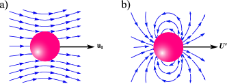
Figure 2: Two different hydrodynamic problems are used in reciprocal theorem to achieve the swimming velocity of a Janus particle. a) Problem i@: the velocity field of a translating sphere with velocity $u_{\@slowromancap i@}{\bf\hat{z}}$, b) Problem ii@: the velocity field of a self propelling Janus particle with slip velocity given by Equation 22, in laboratory reference frame.

After calculating the propulsion velocity, we can investigate the velocity field due to the self propulsion of this single motor. The above approach works only for evaluating the particle speed. In order to obtain the velocity field we should solve the Stocks equation with proper boundary conditions. A direct solution to the hydrodynamic equations, presented at appendix A, reveals that the velocity field of a self propelled Janus particle in the laboratory frame reads as:

$${\bf V^{\prime}}=\frac{1}{2}\frac{1}{r^{3}}U^{\prime}\left(2\cos\theta\ {\bf\hat{r}}+\sin\theta\ {\bf\hat{\theta}}\right)=-\frac{1}{2}\frac{1}{r^{3}}{\bf U^{\prime}}\cdot\left(\mathbb{I}-3{\bf\hat{r}}{\bf\hat{r}}\right).$$ (30)

One should note that the above velocity field, resembles the velocity field due to a dipole of sink and source of potential flow. As a result of the force free condition, we had this expectation from the beginning, that in a multipole expansion of the velocity field, the source dipole should have the dominant effect.

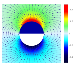
Figure 3: Ionic density profile and fluid velocity streamlines of an electrokinetic self propelled Janus particle. Asymmetric distribution of ions and slip velocity on the surface are essential elements that cause the Janus particle to move.

VI Two Interacting Janus particles

As shown in Figure 4, let us consider two spherically symmetric Janus particles with radii $a_{1}$ and $a_{2}$. These two particles are separated by a center to center vector denoted by ${\bf D}$. The position of a general point in space with respect to each motor is given by ${\bf r}_{1(2)}$, respectively. Intrinsic propulsion velocities of Janus particles point along the directions given by ${\bf\hat{t}}_{1(2)}$. In reference frames that are locally connected to each spheres, the polar angles are measured with respect to ${\bf\hat{t}}_{1,2}$ and are denoted by $\theta_{1,2}$ and $\varphi_{1,2}$. The surface activity of the Janus particles are given by:

$${\bf\hat{n}}_{i}\cdot{\bf j}_{\pm}({\bf r}_{i}=a_{i}{\hat{\bf n}}_{i})={\dot{Q}}_{i}\cos\theta_{i},~{}~{}~{}i=1,2,$$

where ${\bf\hat{n}}_{1}$ and ${\bf\hat{n}}_{2}$ represent the unit vectors that are normal to the spheres and the ionic production rates at the surfaces of motors are denoted by ${\dot{Q}}_{1}$ and ${\dot{Q}}_{2}$. As a result of the calculation given at previous section, the intrinsic propulsion speed of motors, which are the speed of isolated motors, are given by Equation 28. We want to calculate the influences of a Janus particle on the speed of a nearby Janus particle.

At the limit of very small Debye layer, the case that we are interested here, the electric effects of particles are screened and the direct electrostatic interaction between the particles can be neglected. In this case, the electro-hydrodynamic forces should be considered.

Neglecting the direct electrostatic interaction between particles, two types of effects can mediate the electro-hydrodynamic forces. Both the direct hydrodynamic interaction between moving particles immersed in the fluid medium and also the change of fluid pattern due to the rearrangement of ionic species which are subjected to instantaneous boundary condition on both particles, will eventually lead to coupling between Janus particles. For simplicity, we call the former case by direct and denote the latter case by indirect contributions. The direct (indirect) interaction, is due to the instantaneous appearance of particle positions in the boundary conditions of hydrodynamic (electrostatic) equations.

It is very important to note that both kinds of the above interactions are of hydrodynamics in nature and it is the fluid medium that mediates both types of the interactions. As an approximation, we assume that these two contributions are additive. The validity of this approximation is guaranteed for very far separated particles and we will clarify it in more details at the following sections.

Denoting the overall translational and rotational velocities of each particles by ${\bf U}_{i}$ and $\Omega_{i}$, we can write them as:

$${\bf U}_{i} = {\bf U}_{i}^{0}+{\bf U}_{i}^{\text{dir}}+{\bf U}_{i}^{\text{ind}},$$

$${\bf\Omega}_{i} = {\bf\Omega}_{i}^{0}+{\bf\Omega}_{i}^{\text{dir}}+{\bf\Omega}_{i}^{\text{ind}},$$ (31)

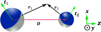
Figure 4: Geometry of two spherical self propelled Janus particles that are located in distance ${\bf D}$.

where the intrinsic translational and rotational propulsion velocities of the $i^{\prime}$th Janus particle are given by:

$${\bf U}^{0}_{i}=\frac{4}{3}{\dot{Q}}_{i}\ln\left(\cosh\frac{\zeta_{i}}{4}\right){\bf{\hat{t}}}_{i},~{}~{}~{}{\bf\Omega}_{i}^{0}=0.$$ (32)

From here, we use the radius of the first sphere $a_{1}$ for making dimensionless lengths. This means that our results will depend on a new dimensionless number $e=\left(a_{2}/a_{1}\right)$.

We aim to calculate the direct and indirect contributions. As described before, the coupling between two particles arises from the boundary conditions that take into account the positions of two particles. The ionic concentration field satisfies the Poisson equation and it is subjected to boundary conditions on the outer part of the Debye layer of both Janus particles. In the limit of thin Debye layer with $\delta\rightarrow 0$, the Poisson equation simplifies to ${\bf\nabla}^{2}N=0$, where $N({\bf r}_{1},{\bf r}_{2})$ shows the ionic concentration outside the Debye layer (effective properties of bulk). The ionic concentration satisfies the following boundary conditions:

$$\frac{\partial N}{\partial r_{i}}=-{\dot{Q}}_{i}\cos\theta_{i},~{}~{}~{}~{}~{}~{}{\bf r}_{i}=\hat{{\bf n}}_{i},~{}~{}~{}~{}i=1,2.$$ (33)

In addition to the above boundary conditions, the velocity field also should satisfy the Dukhin-Derjaguin slip velocity on the outer surface of Debye layer of each particles. The hydrodynamic boundary conditions read:prieve1

$${\bf V}_{S_{i}}=-4\ln\left(\cosh\frac{\zeta_{0_{i}}}{4}\right){\bf\nabla}_{S_{i}}N,~{}~{}~{}{\bf r}_{i}=\hat{{\bf n}}_{i},~{}~{}i=1,2,$$ (34)

where the tangential gradient operator is denoted by ${\bf\nabla}_{S_{i}}$.

Simultaneous application of two boundary conditions given by Equation 33 and Equation 34, is the main difficulty that makes it impossible to present a full analytic solution. In the limit of very far motors, $D\gg 1,e\sim 1$, we can proceed with a perturbation method. We first assume that the motors are hydrodynamically uncoupled and assume that the coupling is only due to the boundary condition on the ionic concentration. This will give us the indirect contribution. Then to obtain an approximation for the direct hydrodynamic contribution, we assume that the motors are decoupled with respect to ionic boundary conditions, and investigate the hydrodynamic boundary conditions separately. This scheme will provide us a systematic way to expand the interaction in powers of $1/D$.

In the following, we first calculate the indirect contribution and then the direct hydrodynamic contribution is also calculated.

VI.1 Indirect contribution

To obtain the indirect contribution, we should take into account the boundary condition on concentration field that is given by Equation 33. For very far particles ($D\gg 1$), we denote the concentration profiles for isolated particles by: $N_{1}^{0}$ and $N_{2}^{0}$. In this case we can write the real concentration field that obeys the full boundary conditions as:

$$N=N_{1}^{0}+N_{2}^{0}+\Delta N,$$ (35)

where the deviations from isolated particle solution is denoted by: $\Delta N$. As have been calculated in previous sections, the concentration profiles for isolated particles are given by:

$$N_{1}^{0}=\frac{{\dot{Q}}_{1}}{2r_{1}^{2}}\cos\theta_{1},~{}~{}N_{2}^{0}=\frac{e^{3}{\dot{Q}}_{2}}{2r_{2}^{2}}\cos\theta_{2}.$$ (36)

Writing the deviation from single particle profile as:

$$\Delta N=\sum_{\alpha=1}^{\infty}(N_{1}^{\alpha}+N_{2}^{\alpha})$$ (37)

we can easily see that the new fields satisfy the Laplace equation as $\nabla^{2}N_{i}^{\alpha}=0$ with the boundary conditions given by:

$$\frac{\partial N_{i}^{\alpha}}{\partial n}=-\frac{\partial N_{j}^{\alpha-1}}{\partial n},~{}~{}~{}~{}~{}{\bf r}_{i}=\hat{{\bf n}}_{i},~{}~{}~{}~{}i,j=1,2.$$ (38)

Such hierarchical description of the effects of motors, allow us to develop a systematic expansion in powers of $1/D$.

At the leading order of calculations, we can proceed by considering the zero order term. Having in hand the zero order concentration profile, we can use Equation 34 and evaluate the slip velocities on the surface of each motors. Performing such calculations, we can arrive at the following relations for the slip velocities. On the surface of first Janus particle, and in the laboratory reference frame, the velocity reads as:

$${\bf V}_{S_{1}}^{\text{ind}}=-\frac{3}{2}{\bf U}_{1}^{0}\cdot\left(\mathbb{I}-{\bf\hat{r}}_{1}{\bf\hat{r}}_{1}\right)$$

$$-\frac{3}{2}\frac{e^{3}}{D^{3}}\ {\bf U}_{2}^{0}\cdot\left(\mathbb{I}-3{\bf\hat{D}}{\bf\hat{D}}\right)\cdot\left(\mathbb{I}-{\bf\hat{r}}_{1}{\bf\hat{r}}_{1}\right)$$

$$+\frac{9}{2}\frac{e^{3}}{D^{4}}\ {\bf U}_{2}^{0}\cdot\left(-2\mathbb{I}+5{\bf\hat{D}}{\bf\hat{D}}\right)\cdot{\bf\hat{r}}_{1}{\bf\hat{D}}\cdot\left(\mathbb{I}-{\bf\hat{r}}_{1}{\bf\hat{r}}_{1}\right)$$

$$-\frac{9}{2}\frac{e^{3}}{D^{4}}\ {\bf\hat{r}}_{1}\times({\bf U}_{2}^{0}\times{\bf\hat{D}}),$$ (39)

and on the surface of second Janus particle, the slip velocity reads as:

$${\bf V}_{S_{2}}^{\text{ind}}=-\frac{3}{2}\frac{1}{e^{3}}\ {\bf U}_{2}^{0}\cdot\left(\mathbb{I}-{\bf\hat{r}}_{2}{\bf\hat{r}}_{2}\right)$$

$$-\frac{3}{2}\frac{1}{D^{3}}\ {\bf U}_{1}^{0}\cdot\left(\mathbb{I}-3{\bf\hat{D}}{\bf\hat{D}}\right)\cdot\left(\mathbb{I}-{\bf\hat{r}}_{2}{\bf\hat{r}}_{2}\right)$$

$$-\frac{9}{2}\frac{e}{D^{4}}\ {\bf U}_{1}^{0}\cdot\left(-2\mathbb{I}+5{\bf\hat{D}}{\bf\hat{D}}\right)\cdot{\bf\hat{r}}_{2}{\bf\hat{D}}\cdot\left(\mathbb{I}-{\bf\hat{r}}_{2}{\bf\hat{r}}_{2}\right)$$

$$+\frac{9}{2}\frac{e}{D^{4}}\ {\bf\hat{r}}_{2}\times({\bf U_{1}^{0}}\times{\bf\hat{D}}).$$ (40)

As one can see, the slip velocity on each particle has two contributions. As an example and, for the first particle, these two contributions are the term that is proportional to ${\bf U}_{1}^{0}$ and the terms that are proportional to ${\bf U}_{2}^{0}$. The first term denotes the intrinsic asymmetry of the particle while, the other parts are due to the asymmetry of the second Janus particle.

As a result of the above surface slip velocities, the velocity filed in the medium deviates from its value for the isolated Janus particles. Now to obtain the full changes in the velocity field, we need to apply the full hydrodynamic boundary conditions on both particle. Here, we want to neglect such complexities and simply assume that the velocity profile is still due to the isolated Janus particles but with modified slip velocities given by the above relations. This is the core of our direct-indirect separation of the effects and what we obtain with this assumption, contains the indirect contribution. At the next section, we will again come back to this point and take into account the effects that we neglected here.

We write the fluid velocity field in the laboratory frame as:

$${\bf V}^{\text{ind}}={\bf V}_{1}^{\text{ind}}+{\bf V}_{2}^{\text{ind}},$$ (41)

where the partial flows due to each Janus particles can be written as:

$${\bf V}_{1}^{\text{ind}}=-\frac{1}{2}\frac{1}{r_{1}^{3}}\left({\bf U}_{1}^{0}+{\bf U}_{1}^{\text{ind}}\right)\cdot\left(\mathbb{I}-3{\bf\hat{r}}_{1}{\bf\hat{r}}_{1}\right)+{\cal O}(\frac{1}{r_{1}})^{4},$$

$${\bf V}_{2}^{\text{ind}}=-\frac{1}{2}\frac{e^{3}}{r_{2}^{3}}\left({\bf U}_{2}^{0}+{\bf U}_{2}^{\text{ind}}\right)\cdot\left(\mathbb{I}-3{\bf\hat{r}}_{2}{\bf\hat{r}}_{2}\right)+{\cal O}(\frac{1}{r_{2}})^{4},$$

where the velocity contributions that the particles achieved from indirect interaction are denoted by: ${\bf U}_{i}^{\text{ind}}$ and ${\bf\Omega}_{i}^{\text{ind}}$. The above relations are essentially the velocity profiles of isolated Janus particles given in equation 30, but with modified swimming velocities.

Two important conditions of zero total force and zero total torque, are essential points that we should apply to the equations for obtaining ${\bf U}_{i}^{\text{ind}}$ and ${\bf\Omega}_{i}^{\text{ind}}$. Similar to the case of a single Janus particle, we can use the Lorentz reciprocal theorem and extract the required results. The details of such calculations are collected in appendix B. For the first particle, the final results read:

$${\bf U}_{1}^{\text{ind}} = \frac{e^{3}}{D^{3}}U_{2}^{0}\ {\bf\hat{t}}_{2}\cdot\left(\mathbb{I}-3{\bf\hat{D}}{\bf\hat{D}}\right)$$

$${\bf\Omega}_{1}^{\text{ind}} = -\frac{9}{2}\frac{e^{3}}{D^{4}}U_{2}^{0}\left({\bf\hat{t}}_{2}\times{\bf\hat{D}}\right),$$ (43)

and for the second particle, we will have:

$${\bf U}_{2}^{\text{ind}} = \frac{1}{D^{3}}U_{1}^{0}\ {\bf\hat{t}}_{1}\cdot\left(\mathbb{I}-3{\bf\hat{D}}{\bf\hat{D}}\right)$$

$${\bf\Omega}_{2}^{\text{ind}} = \frac{9}{2}\frac{e}{D^{4}}U_{1}^{0}\left({\bf\hat{t}}_{1}\times{\bf\hat{D}}\right).$$ (44)

The above results, present the zero order indirect contributions, regarding the perturbation expansion introduced in equation 35. As one can see, the results for transnational velocity decays like $(1/D)^{3}$. To see the effects of the next order terms, we need to solve the Laplace equation for $N_{i}^{1}$ with proper boundary condition given by Equation 38. As the boundary condition decays like $(1/D)^{2}$ and the governing equation is also linear, we will expect such a similar decay for $N_{i}^{1}$. Now for calculating the effects of such first order term in the velocities, we should repeat the same procedure as described for zero order term. Continuing the calculations, we will eventually receive at a velocity correction for Janus particles that decays like $(1/D)^{3}\times(1/D)^{2}$. At the next part, we will show that the direct hydrodynamic contribution give corrections that are more effective than these corrections. So we will ignore the higher order corrections due to the concentration profile and keep only the zero order contribution.

VI.2 Direct hydrodynamic contribution

In the previous section, we have neglected the complexities associated with simultaneous applications of the slip velocity condition on both particles. We have simply assumed that the velocity profile corresponds to the isolated Janus particles but with modified slip velocities. Here, we want to go beyond this simplifications and obtain the corrections associated to such complexities. To achieve the overall velocity field ${\bf V}$, associated to the complete problem that takes into account both direct and indirect interactions, a Stokes equation with the following boundary conditions on the surface of Janus particles should be solved:

$${\bf V}|_{S_{1}}={\bf U}_{1}^{0}+{\bf U}_{1}^{\text{ind}}+{\bf\Omega}_{1}^{\text{ind}}\times{\bf r}_{1}+{\bf U}_{1}^{\text{dir}}+{\bf\Omega}_{1}^{\text{dir}}\times{\bf r}_{1}+{\bf V}_{S_{1}}^{\text{ind}}$$

$${\bf V}|_{S_{2}}={\bf U}_{2}^{0}+{\bf U}_{2}^{\text{ind}}+{\bf\Omega}_{2}^{\text{ind}}\times({\bf r}_{1}-{\bf D})$$

$$~{}~{}~{}~{}~{}~{}~{}~{}~{}+{\bf U}_{2}^{\text{dir}}+{\bf\Omega}_{2}^{\text{dir}}\times({\bf r}_{1}-{\bf D})+{\bf V}_{S_{2}}^{\text{ind}}$$

$${\bf V}|_{\infty}=0,$$ (45)

where we have assumed that as a result of hydrodynamic interaction between the particles, each Janus particle achieve an additional change in its velocities given by: ${\bf U}_{i}^{\text{dir}}$ and ${\bf\Omega}_{i}^{\text{dir}}$. Again a proper application of Lorentz reciprocal theorem, will help us to extract the required velocities. The details of calculations are presented in appendix C, and here we write the final results. For the first Janus particle and up to the order ${\cal O}(1/D)^{6}$, we will have:

$${\bf U}_{1}^{\text{dir}} =-\frac{1}{2}\frac{e^{3}}{D^{3}}U_{2}^{0}\ {\bf\hat{t}}_{2}\cdot\left(\mathbb{I}-3{\bf\hat{D}}{\bf\hat{D}}\right),$$ (46)

$$-\frac{1}{2}\frac{e^{3}}{D^{6}}U_{1}^{0}\ {\bf\hat{t}}_{1}\cdot\left(\mathbb{I}-3{\bf\hat{D}}{\bf\hat{D}}\right)\cdot\left(\mathbb{I}-3{\bf\hat{D}}{\bf\hat{D}}\right),$$

the first term that is proportional to $U_{2}^{0}$, is the velocity field produced by the second Janus particle and calculated at the position of first Janus particle. This is a result that we expected to see from the Faxen theorem for a colloidal particle immersed in external velocity field. Calculations show that, the dominant part of the rotational velocity induced by direct interaction, will behave like: $(1/D)^{9}$ and, we neglect it here. Similar expression can be obtained for the second Janus particle that reads as:

$${\bf U}_{2}^{\text{dir}} =-\frac{1}{2}\frac{1}{D^{3}}U_{1}^{0}\ {\bf\hat{t}}_{1}\cdot\left(\mathbb{I}-3{\bf\hat{D}}{\bf\hat{D}}\right),$$ (47)

$$-\frac{1}{2}\frac{1}{D^{6}}U_{2}^{0}\ {\bf\hat{t}}_{2}\cdot\left(\mathbb{I}-3{\bf\hat{D}}{\bf\hat{D}}\right)\cdot\left(\mathbb{I}-3{\bf\hat{D}}{\bf\hat{D}}\right).$$

Very interestingly, the dominant part of both direct and indirect contributions behave similarly for $D\gg 1$. Therefore the dominant part of the total translational and rotational velocity of the first Janus particle is given by:

$${\bf U}_{1} ={\bf U}_{1}^{0}+\frac{1}{2}\frac{e^{3}}{D^{3}}U_{2}^{0}\ {\bf\hat{t}}_{2}\cdot\left(\mathbb{I}-3{\bf\hat{D}}{\bf\hat{D}}\right),$$

$${\bf\Omega}_{1} =-\frac{9}{2}\frac{e^{3}}{D^{4}}U_{2}^{0}\left({\bf\hat{t}}_{2}\times{\bf\hat{D}}\right),$$ (48)

As a result of symmetry, the corresponding velocities of the second Janus particle can be written as:

$${\bf U}_{2} ={\bf U}_{2}^{0}+\frac{1}{2}\frac{1}{D^{3}}U_{1}^{0}\ {\bf\hat{t}}_{1}\cdot\left(\mathbb{I}-3{\bf\hat{D}}{\bf\hat{D}}\right),$$

$${\bf\Omega}_{2} =\frac{9}{2}\frac{e}{D^{4}}U_{1}^{0}\left({\bf\hat{t}}_{1}\times{\bf\hat{D}}\right).$$ (49)

In the next part, we show how such interactions will modify the trajectories of Janus particles.

VII Results and discussion

We have shown that as a result of coupling between hydrodynamic and electrostatic effects, a long-range interaction between particles have been mediated. For a very thin Debye layer $\kappa a\gg 1$ and $a\ll D$, the electrostatic effects of Janus particles are screened and we have neglected the electric interaction of the Janus particles. In this case all the interactions between particles have hydrodynamical origin that is long range. Such long range interaction, affects the translational velocity of each motors, and it also introduces a rotational velocity for motors. For very far Janus particles, the leading order of translational speed scales as ${\cal O}\left([1/D]^{3}\right)$ and angular velocity scales as ${\cal O}\left([1/D]^{4}\right)$. The interaction modifies the trajectories of self propelling Janus particles. To have a qualitative feeling of the interaction, some typical examples of the trajectories are presented in Figure 5. As one can distinguish from figures, the overall effect of the interaction depends on the initial states of two Janus particles. In all trajectories, the dashed-line corresponds to the trajectory of an isolated Janus particle. For the cases where the particles move in same directions (the first two trajectories shown in figure), the interaction has a repulsive signature. But for a case where the particles move in anti-parallel directions (the third trajectory shown in Figure 5), the interaction tends to decrease the relative speed of two particles. We have used the dominant part of the interactions but please note that by using the method that we have developed in this paper, we are able to systematically consider all of the orders of perturbation terms.

Along this work, we are currently working on the dynamics of a collection of active Janus particles. It is a known fact that hydrodynamic interaction near a rough wall will introduce nontrivial effects,rad2010hydrodynamic in this case we are also analyzing the motion of a single Janus motor near a wall with surface roughness.

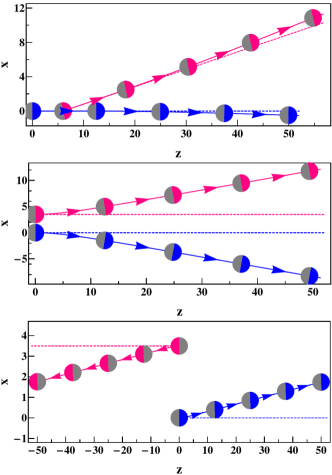
Figure 5: Trajectories of two interacting Janus particles are shown for different initial states of the motors. In all figures the intrinsic speed of the motors are assumed to be similar. As one can see, for the case of two parallel motors, the interaction tends to repel the Janus particles.

Appendix A Velocity field due to a single active Janus particle

In this appendix, we present the detail of the calculations for the velocity field produced by a moving single Janus motor. Along this task, we should solve the Stocks equation, with boundary conditions given as follows:

$${\bf V^{\prime}}|_{\infty} =-U^{\prime}{\bf\hat{z}}=-U^{\prime}\cos\theta\ {\bf\hat{r}}+U^{\prime}\sin\theta\ {\hat{\boldsymbol{\theta}}},$$

$${\bf V^{\prime}}|_{r=1} =-4\ln\left(\cosh\frac{\zeta_{0}}{4}\right)\nabla_{S}N^{\prime}|_{r=1}$$

$$=\frac{3}{2}U^{\prime}\sin\theta\ {\bf\hat{\theta}}.$$

To proceed, we eliminate the pressure field from the Stokes equation by evaluating the curl of this equation. This will gives us:

$$\nabla\times(\nabla^{2}{\bf V^{\prime}})=\nabla^{2}(\nabla\times{\bf V^{\prime}})=0.$$

In terms of stream function $H(r,\theta)$, the velocity field can be written as:

$${\bf V^{\prime}}=\frac{1}{r\sin\theta}\frac{\partial H}{\partial r}\ {\hat{\boldsymbol{\theta}}}-\frac{1}{r^{2}\sin\theta}\frac{\partial H}{\partial\theta}\ {\bf\hat{r}},$$

where the incompressibility condition $\nabla\cdot{\bf V^{\prime}}=0$, is assumed. According to the boundary condition at infinity, one can suggest a solution for $H$ as:

$$H(r,\theta)=f(r)\sin^{2}\theta.$$

using the above ansatz, the curl of velocity field reads as:

$$\nabla\times\mathbf{V^{\prime}} =\left(\dfrac{1}{r}\dfrac{d^{2}f}{dr^{2}}-\dfrac{2}{r^{3}}f\right)\sin\theta\ {\hat{\boldsymbol{\varphi}}}$$

$$=A(r)\sin\theta\ {\hat{\boldsymbol{\varphi}}},$$

where $A(r)=\dfrac{1}{r}\dfrac{d^{2}f}{dr^{2}}-\dfrac{2}{r^{3}}f$. Now we can write:

$$\nabla^{2}(\nabla\times\mathbf{V^{\prime}})={\hat{\boldsymbol{\varphi}}}\ \sin\theta\left[\dfrac{d^{2}A}{dr^{2}}+\dfrac{2}{r}\dfrac{dA}{dr}-\dfrac{2A}{r^{2}}\right]=0.$$

So we have following equation for $A(r)$:

$$\dfrac{d^{2}A}{dr^{2}}+\dfrac{2}{r}\dfrac{dA}{dr}-\dfrac{2A}{r^{2}}=0,$$

and its solution is:

$$A=B^{\prime}_{1}r+\dfrac{B^{\prime}_{2}}{r^{2}},$$

where $B^{\prime}_{1}$, $B^{\prime}_{2}$ are integration constants. Function $f$ satisfies the following differential equation:

$$\dfrac{d^{2}f}{dr^{2}}-\dfrac{2}{r^{2}}f-B^{\prime}_{1}r^{2}+\dfrac{B^{\prime}_{2}}{r}=0,$$

which has a general solution like:

$$f=B_{1}r^{4}+B_{2}r+C_{1}r^{2}+\dfrac{C_{2}}{r}.$$

Collecting all the above results, we can write the fluid velocity field as:

$${\bf V}^{\prime}=-\frac{2}{r^{2}}\left(B_{1}r^{4}+B_{2}r+C_{1}r^{2}+\frac{C_{2}}{r}\right)\cos\theta\ {\bf\hat{r}}$$

$$+\frac{1}{r}\left(4B_{1}r^{3}+B_{2}+2C_{1}r-\frac{C_{2}}{r^{2}}\right)\sin\theta\ {\hat{\boldsymbol{\theta}}},$$

where $B_{1}$, $B_{2}$, $C_{1}$ and $C_{2}$ are constants that can be easily determined by applying the boundary conditions. Finally, the fluid velocity field due to a moving Janus particle in a co-moving reference frame reads as:

$${\bf V^{\prime}} =-U^{\prime}\ {\bf\hat{z}}+\frac{1}{2}\frac{U^{\prime}}{r^{3}}\left(2\cos\theta\ {\bf\hat{r}}+\sin\theta\ {\hat{\boldsymbol{\theta}}}\right)$$

$$=-{\bf U^{\prime}}-\frac{1}{2}{\bf U^{\prime}}\cdot\left(\frac{\mathbb{I}-3{\bf\hat{r}}{\bf\hat{r}}}{r^{3}}\right).$$

Appendix B Indirect contribution to the interaction

In this appendix we present the calculations that give the indirect contribution to the interaction between two Janus particles. We just consider the contribution to the velocity of the first motor, then the symmetry arguments will help us to write the velocity change of the second motor as well. As in the case of a single Janus particle, we will benefit the Lorentz reciprocal theorem to extract the indirect contribution. To use the reciprocal theorem, we need to define the set of two hydrodynamic problems which share a common geometry but with different boundary conditions. Let’s start with defining the problem II, first. The case II, corresponds to our main problem defined in the section ”indirect contribution”. We put ${\bf V}_{\@slowromancap ii@}={\bf V}^{\text{ind}}$ and it is subjected to the following boundary conditions:

$${\bf V}_{\@slowromancap ii@}|_{S_{1}}={\bf U}_{1}^{0}+{\bf U}_{1}^{\text{ind}}+{\bf\Omega}_{1}^{\text{ind}}\times{\bf r}_{1}+{\bf V}_{S_{1}}^{\text{ind}},$$

where we would like to find ${\bf U}_{1}^{\text{ind}}$ and ${\bf\Omega}_{1}^{\text{ind}}$ and note that the calculations should be done in laboratory frame. Here ${\bf V}_{S_{1}}^{\text{ind}}$ is the slip velocity given by Equation VI.1, and ${\bf U}_{1}^{0}$ is the first particle velocity from Equation 32.

As we are looking for 6 unknown variables (the components of ${\bf U}_{1}^{\text{ind}}$ and ${\bf\Omega}_{1}^{\text{ind}}$), we can consider 6 different choices for problem i@. To evaluate 3 components for ${\bf U}_{1}^{\text{ind}}$, we choose ${\bf V}_{\@slowromancap i@}$ as the velocity field of a translating particle with velocity $u_{\@slowromancap i@}$ in the three major Cartesian directions, and in order to evaluate 3 components of ${\bf\Omega}_{1}^{\text{ind}}$, we choose the velocity field of a rotating particle with velocity $\omega_{\@slowromancap i@}$ in the three major directions. On the surface of the first particle, we have ${\bf V}_{\@slowromancap i@}|_{S_{1}}={\bf u}_{\@slowromancap i@}+{\boldsymbol{\omega}}_{\@slowromancap i@}\times{\bf r}_{1}$, where:

$$({\bf u}_{\@slowromancap i@},{\boldsymbol{\omega}}_{\@slowromancap i@})_{j=1}=(u_{\@slowromancap i@}{\bf\hat{x}},0),~{}~{}~{}~{}~{}({\bf u}_{\@slowromancap i@},{\boldsymbol{\omega}}_{\@slowromancap i@})_{j=4}=(0,\omega_{\@slowromancap i@}{\bf\hat{x}}),$$

$$({\bf u}_{\@slowromancap i@},{\boldsymbol{\omega}}_{\@slowromancap i@})_{j=2}=(u_{\@slowromancap i@}{\bf\hat{y}},0),~{}~{}~{}~{}~{}({\bf u}_{\@slowromancap i@},{\boldsymbol{\omega}}_{\@slowromancap i@})_{j=5}=(0,\omega_{\@slowromancap i@}{\bf\hat{y}}),$$

$$({\bf u}_{\@slowromancap i@},{\boldsymbol{\omega}}_{\@slowromancap i@})_{j=3}=(u_{\@slowromancap i@}{\bf\hat{z}},0),~{}~{}~{}~{}~{}({\bf u}_{\@slowromancap i@},{\boldsymbol{\omega}}_{\@slowromancap i@})_{j=6}=(0,\omega_{\@slowromancap i@}{\bf\hat{z}}),$$

where $j=1,~{}2,~{}3$ denote the cases of translation along the directions ${\bf\hat{x}},{\bf\hat{y}}$ and ${\bf\hat{z}}$, respectively, and $j=4,~{}5,~{}6$ denote the corresponding cases for rotations along ${\bf\hat{x}},{\bf\hat{y}}$ and ${\bf\hat{z}}$. Note that for all of the above 6 cases, on the surface of the second particle we have: ${\bf V}_{\@slowromancap i@}|_{S_{2}}=0$. Substituting these choices into the left-hand-side of Equation 23, we will obtain:

$$\int{\bf V}_{I}\cdot{\boldsymbol{\sigma}}_{II}\cdot{\bf\hat{n}}\ dS=\int_{S_{1}}\left({\bf u}_{\@slowromancap i@}+{\boldsymbol{\omega}}_{\@slowromancap i@}\times{\bf r}_{1}\right)\cdot{\boldsymbol{\sigma}}_{\@slowromancap ii@}\cdot{\bf\hat{n}}\ dS,$$

$$={\bf u}_{\@slowromancap i@}\cdot\int_{S_{1}}{\boldsymbol{\sigma}}_{\@slowromancap ii@}\cdot{\bf\hat{n}}\ dS+{\boldsymbol{\omega}}_{\@slowromancap i@}\cdot\int_{S_{1}}{\bf r}_{1}\times{\boldsymbol{\sigma}}_{\@slowromancap ii@}\cdot{\bf\hat{n}}\ dS,$$

$$={\bf u}_{\@slowromancap i@}\cdot{\bf F}_{1}+{\boldsymbol{\omega}}_{\@slowromancap i@}\cdot{\bf L}_{1}=0,$$

where ${\bf F}_{\@slowromancap ii@}$ and ${\bf L}_{\@slowromancap ii@}$ are the force and torque exerted on the particle 1 and are equal to zero. Then from the right-hand-side of Equation 23 we have:

$$\left({\bf U}_{1}^{0}+{\bf U}_{1}^{\text{ind}}\right)\cdot\int_{S_{1}}{\boldsymbol{\sigma}}_{\@slowromancap i@}\cdot{\bf\hat{n}}\ dS\ +\ {\bf\Omega}_{1}^{\text{ind}}\cdot\int_{S_{1}}{\bf r}_{1}\times{\boldsymbol{\sigma}}_{\@slowromancap i@}\cdot{\bf\hat{n}}\ dS,$$

$$+\ \int_{S_{1}}{\bf V}_{S_{1}}^{\text{ind}}\cdot{\boldsymbol{\sigma}}_{\@slowromancap i@}\cdot{\bf\hat{n}}\ dS=0,$$

where ${\bf F}_{\@slowromancap i@}=\int_{S_{1}}{\boldsymbol{\sigma}}_{\@slowromancap i@}\cdot{\bf\hat{n}}\ dS$ and ${\bf L}_{\@slowromancap i@}=\int_{S_{1}}{\bf r}_{1}\times{\boldsymbol{\sigma}}_{\@slowromancap i@}\cdot{\bf\hat{n}}\ dS$ are the force and torque exerted on the particle in the problem i@. Now for the first three problems ($j=1,~{}2,~{}3$) which:

$${\boldsymbol{\omega}}_{\@slowromancap i@}=0,~{}~{}~{}~{}{\bf F}_{\@slowromancap i@}=-6\pi{\bf u}_{\@slowromancap i@},~{}~{}~{}~{}{\bf L}_{\@slowromancap i@}=0,~{}~{}~{}~{}{\boldsymbol{\sigma}}_{\@slowromancap i@}\cdot{\bf\hat{n}}=-\frac{3}{2}{\bf u}_{\@slowromancap i@},$$

we have:

$$-6\pi\left({\bf U}_{1}^{0}+{\bf U}_{1}^{\text{ind}}\right)\cdot{\bf u}_{\@slowromancap i@}+\ \int_{S_{1}}{\bf V}_{S_{1}}^{\text{ind}}\cdot{\boldsymbol{\sigma}}_{\@slowromancap i@}\cdot{\bf\hat{n}}\ dS=0,$$

and

$$\int_{S_{1}}{\bf V}_{S_{1}}^{\text{ind}}\cdot{\boldsymbol{\sigma}}_{\@slowromancap i@}\cdot{\bf\hat{n}}\ dS=-\frac{3}{2}\left(\int_{S_{1}}{\bf V}_{S_{1}}^{\text{ind}}dS\right)\cdot{\bf u}_{\@slowromancap i@},$$

$$=-6\pi{\bf U}_{1}^{0}\cdot{\bf u}_{\@slowromancap i@}-6\pi\frac{a_{2}^{3}}{D^{3}}{\bf U}_{2}^{0}\cdot\left(\mathbb{I}-3{\bf\hat{D}}{\bf\hat{D}}\right)\cdot{\bf u}_{\@slowromancap i@}.$$

Thus the desired velocity due to indirect interaction is obtained as follows:

$${\bf U}_{1}^{\text{ind}}=\frac{e^{3}}{D^{3}}U_{2}^{0}\ {\bf\hat{t}}_{2}\cdot\left(\mathbb{I}-3{\bf\hat{D}}{\bf\hat{D}}\right).$$

With similar calculations for the other three problems ($j=3,~{}4,~{}5$), we can find ${\bf\Omega}_{1}^{\text{ind}}$ as follows:

$${\bf\Omega}_{1}^{\text{ind}}=-\frac{9}{2}\frac{e^{3}}{D^{4}}U_{2}^{0}\left({\bf\hat{t}}_{2}\times{\bf\hat{D}}\right).$$

Similarly, for the second particle we have:

$${\bf U}_{2}^{\text{ind}}=\frac{1}{D^{3}}U_{1}^{0}\ {\bf\hat{t}}_{1}\cdot\left(\mathbb{I}-3{\bf\hat{D}}{\bf\hat{D}}\right),$$

$${\bf\Omega}_{2}^{\text{ind}}=\frac{9}{2}\frac{e}{D^{4}}U_{1}^{0}\left({\bf\hat{t}}_{1}\times{\bf\hat{D}}\right).$$

Appendix C Direct contribution to the interaction

We have denoted the overall velocity field of the full problem of interacting Janus particles by ${\bf V}$ and, it is constrained to the boundary conditions given by Equation VI.2. Here we apply the reciprocal theorem to extract the direct hydrodynamic interaction between Janus particles. In the absence of direct hydrodynamic interaction, we denote the velocity field produced by the second Janus particle as: ${\bf u}_{\infty}({\bf r})$. The first Janus particle is floated in this filed and it is subjected to a proper boundary conditions. To use the reciprocal theorem, we consider the case of problem ii@ as ${\bf V}_{\@slowromancap ii@}={\bf V}-{\bf u}_{\infty}({\bf r})$ and it is subjected to the following conditions:

$${\bf V}_{\@slowromancap ii@}|_{S_{1}}={\bf U}_{1}^{0}+{\bf U}_{1}^{\text{ind}}+{\bf\Omega}_{1}^{\text{ind}}\times{\bf r}_{1}+{\bf V}_{S_{1}}^{\text{ind}}$$

$$~{}~{}~{}~{}~{}~{}~{}~{}~{}+{\bf U}_{1}^{\text{dir}}+{\bf\Omega}_{1}^{\text{dir}}\times{\bf r}_{1}-{\bf u}_{\infty}(0)$$

$${\bf V}_{\@slowromancap ii@}|_{S_{2}}=0.$$

where ${\bf u}_{\infty}(0)$ is the flow field due to the second particle given at the center of the first particle. ${\bf U}_{1}^{\text{ind}}$ and ${\bf\Omega}_{1}^{\text{ind}}$ are the first janus particle velocities due to the indirect hydrodynamic interaction and ${\bf V}_{S_{1}}^{\text{ind}}$ is the slip condition that is given by Equation VI.1. Velocities ${\bf U}_{1}^{\text{dir}}$ and ${\bf\Omega}_{1}^{\text{dir}}$ are unknowns that we want to find. So we have six unknown components and we should apply Lorentz theorem six times, as we did in appendix B. We consider the problem of case i@, as a spherical particle which moves with constant translational and rotational velocities given by: ${\bf u}_{I}$ and ${\boldsymbol{\omega}}_{I}$. This sphere is immersed in an external velocity field given by: ${\bf u}_{\infty}({\bf r})$ and it is subjected to no slip boundary condition. Therefore, in the laboratory reference frame, on the surface of Janus particles we have: ${\bf V}_{\@slowromancap i@}|_{S_{1}}={\bf u}_{\@slowromancap i@}+{\boldsymbol{\omega}}_{\@slowromancap i@}\times{\bf r}_{1}-{\bf u}_{\infty}(0)$ and ${\bf V}_{\@slowromancap i@}|_{S_{2}}=0$. To evaluate the different components of unknown velocities, we will choose six different choices for ${\bf u}_{I}$ and ${\boldsymbol{\omega}}_{I}$ as have been chosen in appendix B.

Substituting into Equation 23 then, simplifying the results, we will arrive at:

$$\left({\bf U}_{1}^{0}+{\bf U}_{1}^{\text{dir}}+{\bf U}_{1}^{\text{ind}}\right)\cdot{\bf F}_{\@slowromancap i@}+\left({\bf\Omega}_{1}^{\text{dir}}+{\bf\Omega}_{1}^{\text{ind}}\right)\cdot{\bf L}_{\@slowromancap i@}$$

$$=\int_{S_{1}}{\bf u}_{\infty}\cdot{\boldsymbol{\sigma}}_{\@slowromancap i@}\cdot{\bf\hat{n}}\ dS-\int_{S_{1}}{\bf V}_{S_{1}}^{\text{ind}}\cdot{\boldsymbol{\sigma}}_{\@slowromancap i@}\cdot{\bf\hat{n}}\ dS.$$

Now we consider the three problems $j=1,~{}2,~{}3$ (the problems that have been defined in appendix B). So the right-hand-side terms are calculated as:

$$\int_{S_{1}}{\bf u}_{\infty}\cdot{\boldsymbol{\sigma}}_{\text{\@slowromancap i@}}\cdot{\bf\hat{n}}\ dS=-\frac{3}{2}{\bf u}_{\text{\@slowromancap i@}}\cdot\int_{S_{1}}{\bf u}_{\infty}\ dS$$

$$\approx-\frac{3}{2}{\bf u}_{\text{\@slowromancap i@}}\cdot 4\pi\left({\bf u}_{\infty}({\bf r}_{1}=0)+\frac{1}{6}\nabla^{2}{\bf u}_{\infty}({\bf r}_{1}=0)\right)$$

$$\approx-6\pi{\bf u}_{\text{\@slowromancap i@}}\cdot\left(-\frac{1}{2}\frac{e^{3}}{D^{3}}\left({\bf U}_{2}^{0}+{\bf U}_{2}^{\text{ind}}\right)\cdot(\mathbb{I}-3{\bf\hat{D}}{\bf\hat{D}})+{\cal O}\left(\frac{1}{D^{6}}\right)\right),$$

and

$$\int{\bf V}_{S_{1}}^{\text{ind}}\cdot{\boldsymbol{\sigma}}_{\text{\@slowromancap i@}}\cdot{\bf\hat{n}}\ dS$$

$$=-\frac{9}{4}\left({\bf U}_{1}^{0}+{\bf U}_{1}^{\text{ind}}\right)\cdot\int_{S_{1}}({\bf\hat{r}}{\bf\hat{r}}-\mathbb{I})\ d\cos\theta\ d\varphi\cdot{\bf u}_{\text{\@slowromancap i@}}$$

$$=6\pi\left({\bf U}_{1}^{0}+{\bf U}_{1}^{\text{ind}}\right)\cdot{\bf u}_{\text{\@slowromancap i@}},$$

now collecting the above results, we have:

$$-6\pi\left({\bf U}_{1}^{0}+{\bf U}_{1}^{\text{dir}}+{\bf U}_{1}^{\text{ind}}\right)\cdot{\bf u}_{\text{\@slowromancap i@}}=$$

$$-6\pi{\bf U}_{1}^{0}\cdot{\bf u}_{\text{\@slowromancap i@}}-6\pi{\bf U}_{1}^{\text{ind}}\cdot{\bf u}_{\text{\@slowromancap i@}}$$

$$-6\pi\left(-\frac{1}{2}\frac{e^{3}}{D^{3}}\left({\bf U}_{2}^{0}+{\bf U}_{2}^{\text{ind}}\right)\cdot(\mathbb{I}-3{\bf\hat{D}}{\bf\hat{D}})+{\cal O}\left(\frac{1}{D^{6}}\right)\right)\cdot{\bf u}_{\text{\@slowromancap i@}}.$$

The final result for ${\bf U}_{1}^{\text{dir}}$ can be written as:

$${\bf U}_{1}^{\text{dir}} =-\frac{1}{2}\frac{e^{3}}{D^{3}}{\bf U}_{2}^{0}\cdot(\mathbb{I}-3{\bf\hat{D}}{\bf\hat{D}})-\frac{1}{2}\frac{e^{3}}{D^{3}}{\bf U}_{2}^{\text{ind}}\cdot(\mathbb{I}-3{\bf\hat{D}}{\bf\hat{D}})$$

$$+{\cal O}\left(\frac{1}{D^{6}}\right).$$

Now for evaluating ${\bf\Omega^{\text{dir}}}$, we consider three problems given as $j=4,~{}5,~{}6$ in appendix B. For these cases we have:

$${\bf u}_{\@slowromancap i@}=0,~{}~{}~{}~{}{\bf F}_{\@slowromancap i@}=0,~{}~{}~{}~{}{\bf L}_{\@slowromancap i@}=-8\pi{\boldsymbol{\omega}}_{\@slowromancap i@},~{}~{}~{}~{}{\boldsymbol{\sigma}}_{\@slowromancap i@}\cdot{\bf\hat{n}}=-3\ {\boldsymbol{\omega}}_{\@slowromancap i@}\times\hat{{\bf r}}_{1}.$$

So the right-hand-side terms of the reciprocal integral are calculated as:

$$\int_{S_{1}}{\bf u}_{\infty}\cdot{\boldsymbol{\sigma}}_{\text{\@slowromancap i@}}\cdot{\bf\hat{n}}\ dS$$

$$=-3\ {\boldsymbol{\omega}}_{\text{\@slowromancap i@}}\cdot\int_{S_{1}}{\bf\hat{r}}\times{\bf u}_{\infty}\ dS$$

$$\approx-3\ {\boldsymbol{\omega}}_{\text{\@slowromancap i@}}\cdot\int_{S_{1}}{\bf\hat{r}}\times\left({\bf u}_{\infty}({\bf r}_{1}=0)+\frac{4\pi}{3}\nabla\times{\bf u}_{\infty}({\bf r}_{1}=0)\right)$$

$$\approx{\cal O}\left(\frac{1}{D^{9}}\right),$$

and

$$\int{\bf V}_{S_{1}}^{\text{ind}}\cdot{\boldsymbol{\sigma}}_{\text{\@slowromancap i@}}\cdot{\bf\hat{n}}\ dS=-3\ {\boldsymbol{\omega}}_{\text{\@slowromancap i@}}\cdot\int_{S_{1}}{\bf\hat{r}}\times{\bf V}_{S_{1}}^{\text{ind}}\ d\cos\theta\ d\varphi$$

$$=-36\pi\frac{e^{3}}{D^{4}}\left({\bf U}_{2}^{0}\times{\bf\hat{D}}\right)\cdot{\boldsymbol{\omega}}_{\text{\@slowromancap i@}},$$

$$=8\pi\ {\bf\Omega}^{\text{ind}}\cdot{\boldsymbol{\omega}}_{\text{\@slowromancap i@}}.$$

Substituting the above results into the reciprocal integral, we can see that:

$$-8\pi\left({\bf\Omega}^{\text{ind}}+{\bf\Omega}^{\text{dir}}\right)\cdot{\boldsymbol{\omega}}_{\text{\@slowromancap i@}}=-8\pi\ {\bf\Omega}^{\text{ind}}\cdot{\boldsymbol{\omega}}_{\text{\@slowromancap i@}}+{\cal O}\left(\frac{1}{D^{9}}\right).$$

This shows that the rotational velocity has no direct contribution behaving stronger than a term like $(1/D)^{9}$.

References

- [1] Euan R Kay, David A Leigh, and Francesco Zerbetto. Synthetic molecular motors and mechanical machines. Angewandte Chemie International Edition, 46(1-2):72–191, 2007.
- [2] Eric Lauga and Thomas R Powers. The hydrodynamics of swimming microorganisms. Reports on Progress in Physics, 72(9):096601, 2009.
- [3] Ali Najafi and Rojman Zargar. Two-sphere low-reynolds-number propeller. Physical Review E, 81(6):067301, 2010.
- [4] Ali Najafi and Ramin Golestanian. Propulsion at low reynolds number. Journal of Physics: Condensed Matter, 17(14):S1203, 2005.
- [5] Jianwei J. Li and Weihong Tan. A single dna molecule nanomotor. Nano Letters, 2(4):315–318, 2002.
- [6] Ivo Buttinoni, Giovanni Volpe, Felix Kümmel, Giorgio Volpe, and Clemens Bechinger. Active brownian motion tunable by light. Journal of Physics: Condensed Matter, 24(28):284129, 2012.
- [7] J Palacci, S Sacanna, S-H Kim, G-R Yi, DJ Pine, and PM Chaikin. Light-activated self-propelled colloids. Philosophical Transactions of the Royal Society of London A: Mathematical, Physical and Engineering Sciences, 372(2029):20130372, 2014.
- [8] Mihail Nicolae Popescu, S Dietrich, M Tasinkevych, and J Ralston. Phoretic motion of spheroidal particles due to self-generated solute gradients. The European Physical Journal E, 31(4):351–367, 2010.
- [9] Ubaldo M. Córdova-Figueroa and John F. Brady. Osmotic propulsion: The osmotic motor. Phys. Rev. Lett., 100:158303, Apr 2008.
- [10] Frank Jülicher and Jacques Prost. Comment on “osmotic propulsion: The osmotic motor”. Phys. Rev. Lett., 103:079801, Aug 2009.
- [11] Edward M Purcell. Life at low reynolds number. Am. J. Phys, 45(1):3–11, 1977.
- [12] Ali Najafi and Ramin Golestanian. Simple swimmer at low reynolds number: Three linked spheres. Physical Review E, 69(6):062901, 2004.
- [13] Walter F Paxton, Kevin C Kistler, Christine C Olmeda, Ayusman Sen, Sarah K St. Angelo, Yanyan Cao, Thomas E Mallouk, Paul E Lammert, and Vincent H Crespi. Catalytic nanomotors: autonomous movement of striped nanorods. Journal of the American Chemical Society, 126(41):13424–13431, 2004.
- [14] Timothy R Kline, Walter F Paxton, Thomas E Mallouk, and Ayusman Sen. Catalytic nanomotors: remote-controlled autonomous movement of striped metallic nanorods. Angewandte Chemie, 117(5):754–756, 2005.
- [15] Jonathan R Howse, Richard AL Jones, Anthony J Ryan, Tim Gough, Reza Vafabakhsh, and Ramin Golestanian. Self-motile colloidal particles: from directed propulsion to random walk. Physical review letters, 99(4):048102, 2007.
- [16] Wei Gao, Allen Pei, and Joseph Wang. Water-driven micromotors. ACS nano, 6(9):8432–8438, 2012.
- [17] Wei Gao, Renfeng Dong, Soracha Thamphiwatana, Jinxing Li, Weiwei Gao, Liangfang Zhang, and Joseph Wang. Artificial micromotors in the mouse’s stomach: A step toward in vivo use of synthetic motors. ACS nano, 9(1):117–123, 2015.
- [18] Aidan Brown and Wilson Poon. Ionic effects in self-propelled pt-coated janus swimmers. Soft matter, 10(22):4016–4027, 2014.
- [19] S Ebbens, DA Gregory, G Dunderdale, JR Howse, Y Ibrahim, TB Liverpool, and R Golestanian. Electrokinetic effects in catalytic pt-insulator janus swimmers. arXiv preprint arXiv:1312.6250, 2013.
- [20] Stephen J Ebbens and Jonathan R Howse. Direct observation of the direction of motion for spherical catalytic swimmers. Langmuir, 27(20):12293–12296, 2011.
- [21] Larysa Baraban, Denys Makarov, Robert Streubel, Ingolf Mönch, Daniel Grimm, Samuel Sanchez, and Oliver G Schmidt. Catalytic janus motors on microfluidic chip: Deterministic motion for targeted cargo delivery. ACS nano, 6(4):3383–3389, 2012.
- [22] Shakuntala Sundararajan, Paul E Lammert, Andrew W Zudans, Vincent H Crespi, and Ayusman Sen. Catalytic motors for transport of colloidal cargo. Nano letters, 8(5):1271–1276, 2008.
- [23] Debabrata Patra, Samudra Sengupta, Wentao Duan, Hua Zhang, Ryan Pavlick, and Ayusman Sen. Intelligent, self-powered, drug delivery systems. Nanoscale, 5(4):1273–1283, 2013.
- [24] Yingjie Wu, Xiankun Lin, Zhiguang Wu, Helmuth Möhwald, and Qiang He. Self-propelled polymer multilayer janus capsules for effective drug delivery and light-triggered release. ACS applied materials & interfaces, 6(13):10476–10481, 2014.
- [25] Daniel Kagan, Rawiwan Laocharoensuk, Maria Zimmerman, Corbin Clawson, Shankar Balasubramanian, Dae Kang, Daniel Bishop, Sirilak Sattayasamitsathit, Liangfang Zhang, and Joseph Wang. Rapid delivery of drug carriers propelled and navigated by catalytic nanoshuttles. Small, 6(23):2741–2747, 2010.
- [26] Fangzhi Mou, Chuanrui Chen, Qiang Zhong, Yixia Yin, Huiru Ma, and Jianguo Guan. Autonomous motion and temperature-controlled drug delivery of mg/pt-poly (n-isopropylacrylamide) janus micromotors driven by simulated body fluid and blood plasma. ACS applied materials & interfaces, 6(12):9897–9903, 2014.
- [27] Yuan Gao and Yan Yu. How half-coated janus particles enter cells. Journal of the American Chemical Society, 135(51):19091–19094, 2013.
- [28] Lluís Soler, Veronika Magdanz, Vladimir M Fomin, Samuel Sanchez, and Oliver G Schmidt. Self-propelled micromotors for cleaning polluted water. ACS nano, 7(11):9611–9620, 2013.
- [29] Beatriz Jurado-Sánchez, Sirilak Sattayasamitsathit, Wei Gao, Luis Santos, Yuri Fedorak, Virendra V Singh, Jahir Orozco, Michael Galarnyk, and Joseph Wang. Self-propelled activated carbon janus micromotors for efficient water purification. Small, 11(4):499–506, 2015.
- [30] Daniel Kagan, Percy Calvo-Marzal, Shankar Balasubramanian, Sirilak Sattayasamitsathit, Kalayil Manian Manesh, Gerd-Uwe Flechsig, and Joseph Wang. Chemical sensing based on catalytic nanomotors: motion-based detection of trace silver. Journal of the American Chemical Society, 131(34):12082–12083, 2009.
- [31] Andreas Walther and Axel HE Müller. Janus particles. Soft Matter, 4(4):663–668, 2008.
- [32] Sébastien Michelin and Eric Lauga. Phoretic self-propulsion at finite péclet numbers. Journal of Fluid Mechanics, 747:572–604, 2014.
- [33] JL Moran, PM Wheat, and JD Posner. Locomotion of electrocatalytic nanomotors due to reaction induced charge autoelectrophoresis. Physical Review E, 81(6):065302, 2010.
- [34] Yasaman Daghighi and Dongqing Li. Micro-valve using induced-charge electrokinetic motion of janus particle. Lab on a Chip, 11(17):2929–2940, 2011.
- [35] Nima Sharifi-Mood, Joel Koplik, and Charles Maldarelli. Diffusiophoretic self-propulsion of colloids driven by a surface reaction: The sub-micron particle regime for exponential and van der waals interactions. Physics of Fluids (1994-present), 25(1):012001, 2013.
- [36] WE Uspal, Mikhail N Popescu, S Dietrich, and M Tasinkevych. Self-propulsion of a catalytically active particle near a planar wall: from reflection to sliding and hovering. Soft matter, 11(3):434–438, 2015.
- [37] Darren G Crowdy. Wall effects on self-diffusiophoretic janus particles: a theoretical study. Journal of Fluid Mechanics, 735:473–498, 2013.
- [38] Alexandra E Frankel and Aditya S Khair. Dynamics of a self-diffusiophoretic particle in shear flow. Physical Review E, 90(1):013030, 2014.
- [39] Ali Najafi and Ramin Golestanian. Coherent hydrodynamic coupling for stochastic swimmers. EPL (Europhysics Letters), 90(6):68003, 2010.
- [40] Majid Farzin, Kiyandokht Ronasi, and Ali Najafi. General aspects of hydrodynamic interactions between three-sphere low-reynolds-number swimmers. Physical Review E, 85(6):061914, 2012.
- [41] CM Pooley, GP Alexander, and JM Yeomans. Hydrodynamic interaction between two swimmers at low reynolds number. Physical review letters, 99(22):228103, 2007.
- [42] S Childress, M Levandowsky, and EA Spiegel. Pattern formation in a suspension of swimming microorganisms: equations and stability theory. Journal of Fluid Mechanics, 69(03):591–613, 1975.
- [43] Christopher Dombrowski, Luis Cisneros, Sunita Chatkaew, Raymond E Goldstein, and John O Kessler. Self-concentration and large-scale coherence in bacterial dynamics. Physical Review Letters, 93(9):098103, 2004.
- [44] Aparna Baskaran and M Cristina Marchetti. Statistical mechanics and hydrodynamics of bacterial suspensions. Proceedings of the National Academy of Sciences, 106(37):15567–15572, 2009.
- [45] Yashodhan Hatwalne, Sriram Ramaswamy, Madan Rao, and R Aditi Simha. Rheology of active-particle suspensions. Physical review letters, 92(11):118101, 2004.
- [46] Moslem Moradi and Ali Najafi. Rheological properties of a dilute suspension of self-propelled particles. EPL (Europhysics Letters), 109(2):24001, 2015.
- [47] LD Landau and EM Lifshitz. Fluid mechanics, vol. 6. Course of Theoretical Physics, pages 227–229, 1987.
- [48] Hiroyuki Ohshima. Theory of colloid and interfacial electric phenomena, volume 12. Academic Press, 2006.
- [49] Ory Schnitzer and Ehud Yariv. Osmotic self-propulsion of slender particles. Physics of Fluids (1994-present), 27(3):031701, 2015.
- [50] Ehud Yariv. Electrokinetic self-propulsion by inhomogeneous surface kinetics. In Proceedings of the Royal Society of London A: Mathematical, Physical and Engineering Sciences, page rspa20100503. The Royal Society, 2010.
- [51] DC Prieve, JL Anderson, JP Ebel, and ME Lowell. Motion of a particle generated by chemical gradients. part 2. electrolytes. Journal of Fluid Mechanics, 148:247–269, 1984.
- [52] John Happel and Howard Brenner. Low Reynolds number hydrodynamics: with special applications to particulate media, volume 1. Springer Science & Business Media, 2012.
- [53] Somaye Hosseini Rad and Ali Najafi. Hydrodynamic interactions of spherical particles in a fluid confined by a rough no-slip wall. Physical Review E, 82(3):036305, 2010.