Data-assimilation by delay-coordinate nudging

Abstract

A new nudging method for data assimilation, delay-coordinate nudging, is presented. Delay-coordinate nudging makes explicit use of present and past observations in the formulation of the forcing driving the model evolution at each time-step. Numerical experiments with a low order chaotic system show that the new method systematically outperforms standard nudging in different model and observational scenarios, also when using an un-optimized formulation of the delay-nudging coefficients. A connection between the optimal delay and the dominant Lyapunov exponent of the dynamics is found based on heuristic arguments and is confirmed by the numerical results, providing a guideline for the practical implementation of the algorithm. Delay-coordinate nudging preserves the easiness of implementation, the intuitive functioning and the reduced computational cost of the standard nudging, making it a potential alternative especially in the field of seasonal-to-decadal predictions with large Earth system models that limit the use of more sophisticated data assimilation procedures.

1 Introduction

State estimation and optimal control theory in geoscience is commonly referred to as data assimilation (DA) (Jazwinski, 1970). The term encompasses the entire sequence of operations that, starting from the observations of a system, and possibly from additional statistical and/or dynamical information (e.g. a model), provides the best-possible estimate of its state (Kalnay, 2002).

DA methods are usually grouped into variational and sequential. In four-dimensional variational (4DVar) DA the model trajectory is adjusted to fit the observations distributed within a given time interval (Sasaki, 1970). The 4DVar, with some specific approximations aimed at reducing its computational cost, has been successfully applied to atmospheric and oceanic models and it is in particular adopted at the European Centre for Medium range Weather Forecast, ECMWF, (Rabier et al., 2000), at Météo-France and at the UK MetOffice. In parallel to the variational approach, ensemble-based methods represent a successful and fruitful alternative. In this case, the DA problem is formulated in a sequential way with a forecast step, where the state estimate and its associated error statistic are propagated in time, alternated with the analyses steps when these estimates are updated using the observations. The ensemble-based schemes are Kalman-filter-like algorithms (Kalman, 1960) in which the error description is obtained using an ensemble of model trajectories aimed at representing the first two moments of the unknown error probability density function. The best-known ensemble-based scheme is the ensemble Kalman filter (EnKF; Evensen (2009)); a version of the EnKF is nowadays operational for the atmospheric model at the Canadian Meteorological Centre, CMC (Houtekamer et al., 2014) and for the ocean system by MET Norway (Sakov et al., 2012). While all these DA methods are formulated in a Gaussian framework, and have proven to work quite well with large-dimensional systems, a new stream of research is nowadays considering the introduction of fully Bayesian procedures (see e.g. (Bocquet et al., 2010)).

Among all sequential DA methods, nudging is probably the simplest one. It is an empirical DA technique, introduced in the early ’70 (see e.g. Anthes (1974); Hoke and Anthes (1976); Lakshmivarahan and Lewis (2013)). The approach, inspired by control system theory (Gelb, 1974), consists in adding a term to the prognostic equations that, acting like an extra-coupling term, drives the model trajectory toward the observations of the unknown system intended to be estimated. The coupling strength is expressed as a relaxation timescale (Macpherson, 1991), and is usually chosen on the basis of the properties of the variable to be nudged.

The empirical origin of nudging has not precluded its formalization and the outline of connections with synchronization problems and Kalman filtering (Duane et al., 2006; Szendro et al., 2009). Methods to estimate systematically the optimal nudging coefficients were proposed by Zou et al. (1992); Stauffer and Bao (1993). This was followed by more sophisticated approaches where the coefficients are made flow-dependent, developed in parallel by meteorological (Vidard et al., 2003; Auroux and Blum, 2008; Auroux, 2009) and dynamical systems (So et al., 1994; Junge and Parlitz, 2001) communities.

A well-known technique of time series analysis consists in the use of delayed coordinates, since this permits the attractor reconstruction from a limited number of observed variables (see e.g. (Kantz and Schreiber, 1997)). The idea of “temporal embedding”, put forward by Packard et al. (1980) and mathematically proven by Takens (1981), has been extraordinary fruitful; and has been recently incorporated into synchronization studies (Abarbanel et al., 2009) (see also (Rey et al., 2014a, b)). This approach, putting aside model errors and observational noise, is based on the expectation that coupling the model to the current and past observations with certain time-dependent nudging coefficients permits full synchronization between model and reality. However, finding the time-dependent nudging coefficients is a hard mathematical task (Rey et al., 2014a, b), with difficult implementation in a realistic model (and certain theoretical limitations (Parlitz et al., 2014)). One example of such difficulties and proposed solution is given in (Rey et al., 2014a), where the Jacobian of the map from physical to the time-delay space is used to compute the forcing terms.

As an alternative, in this paper we investigate a simple albeit effective way of improving the performance of classical nudging, in which nudging coefficients are static and assimilation is performed in a sequential way (i.e. “on the fly”). The new method, named delay-coordinate nudging, makes explicit use of past observations incorporating them to the forcing terms at each time step of the model evolution. The new method systematically outperforms standard nudging (also in the presence of model error), while the increase in computational cost with respect to classical nudging (without delay coordinates) is negligible. Our implementation preserves the easiness of implementation, the intuitive functioning and the reduced computational cost, that have made nudging the preferred choice in the growing field of initialized seasonal-to-decadal predictions with coupled Earth system simulators (Magnusson et al., 2013; Carrassi et al., 2014; Meehl et al., 2013; Doblas-Reyes et al., 2013; Sanchez-Gomez et al., 2015; Servonnat et al., 2015).

Obviously, the number of parameters to be optimized in delay-coordinate nudging is larger than in standard nudging, as the coupling strength at each observation within the delay interval has to be determined, along with the length of the interval itself. However, our numerical results with a low-order nonlinear dynamical system show that by setting the coupling strengths equal at each past observation only slightly deteriorates the performance with respect to the fully optimized case, but with a substantial reduction in the computational cost. Furthermore it is shown that the optimal delay is related to the dominant Lyapunov exponent of the attractor. This provides a physical rationale in support of the delay-coordinates nudging, and a guideline to choose the optimal delay.

The paper is structured as follows: classical and delay-coordinate nudging are described in sections 2 and 3, respectively; numerical results with both perfect and imperfect model setups are reported in sections 4 and 5. Section 6 presents a mathematical argument for the delay-coordinate nudging that is intended to clarify the theoretical basis for the new method. Final conclusions are drawn in section 7.

2 Classical Nudging

We begin by reviewing standard nudging. To simplify the presentation let us consider a spatially discretized system defined in a one-dimensional lattice (e.g. on a latitude circle) and assume that the state of the system at each position is given by a scalar quantity. Furthermore, let ${\mathbf{u}}=(u_{1},u_{2},\ldots,u_{N})$ be the $N$-dimensional state vector representing the unknown system we intend to estimate by doing DA. We assume the ‘truth’ evolves continuously in time and its dynamics be described by the following autonomous dynamical system:

$$\dot{\mathbf{u}}={\mathbf{g}}({\mathbf{u}}),$$ (1)

where upper dot represents the time derivative and ${\mathbf{g}}$ is the vector field. In most applications with practical relevance, only a portion of the system’s state vector is observed, so that observations are performed only at a subset $\cal{M}$ of the $N$ sites; $dim({\cal M})=M<N$. The second key ingredient in DA is the model; it summarizes the knowledge about the unknown dynamics and it is written here under the form of the autonomous dynamical system $\dot{\mathbf{v}}=\tilde{\mathbf{g}}({\mathbf{v}})$, where $\mathbf{v}$ and and $\tilde{\mathbf{g}}$ are the state vector and the vector field of the model, respectively. In the ideal case of a perfect model $\mathbf{v}$ is $N$-dimensional and $\tilde{\mathbf{g}}=\mathbf{g}$.

DA is performed to optimally use the observations and the model in order to “reconstruct” the whole signal, ${\mathbf{u}}$. This accounts to make use of the information contained in the observed areas and gain knowledge on the unobserved ones.

Nudging can be seen as one of the simplest ways to achieve this goal, in a hierarchy of DA procedures of increasing complexity and computational cost (Blayo et al., 2014).

For the sake of focusing on the problem of the spatial sparseness of the observations, we assume hereafter a continuous access to error-free observations, so there is no need for smoothing (i.e. interpolate in time) the observational data.

The classical nudging algorithm consists in introducing a dissipative coupling between the truth and the model (‘master’ and ‘slave’ in the dynamical systems’ jargon):

$$\dot{\mathbf{v}}=\tilde{\mathbf{g}}({\mathbf{v}})+\kappa\mathbf{D}({\mathbf{u}}-{\mathbf{v}})$$ (2)

where $\mathbf{D}$ is a diagonal matrix with elements $D_{ii}=1$ if the $i$-th site is observed, and $D_{ii}=0$ otherwise.

The scalar coefficient $\kappa$ controls the coupling strength and is chosen here to be site-independent because, for the sake of simplicity, the system is assumed to be homogeneous in space and the observed sites are evenly spaced. This situation is typical when running hindcast simulations with an Earth system model nudged toward a reanalysis dataset which gives climate variables on a regular spatial and temporal interval.

The testbed for our discussion and comparison is the Lorenz-96 model (Lorenz, 1996). This classical model is an atmospheric low-order representation of the dynamics of a scalar variable on a circle at equal latitude in the extra-tropics. We shall consider first the case in which the model geometry is a single ring and there is only one temporal scale. The system of $N$ ordinary differential equations governing the truth reads:

$$\dot{u}_{i}=u_{i-1}\left(u_{i+1}-u_{i-2}\right)-u_{i}+F\quad i=1,...,N,$$ (3)

where $i$ runs from $1$ to $N$ with periodic boundary conditions: $u_{0}=u_{N}$, $u_{-1}=u_{N-1}$, $u_{N+1}=u_{1}$. Here, we adopt a system size of $N=60$, and the parameter $F=8$ (unless stated otherwise). With these choices the model behaves with well-developed spatio-temporal chaos (Pazó et al., 2008). The chaotic attractor has $20$ positive Lyapunov exponents, being $\mu\simeq 1.75$ the largest one. The numerical integration of Eq. (3) is performed with an explicit Euler scheme with time step $dt=10^{-3}$, which is hence also the assimilation frequency. We anticipate that, in Sec. 5, we shall investigate the effect of adopting another version of the Lorenz-96 model with two time scales.

In the nudging method the model is coupled to the truth according to the general scheme in Eq. (2). In particular, for a truth given by Eq. (3) we have (in a perfect model scenario)

$$\dot{v}_{i}=v_{i-1}\left(v_{i+1}-v_{i-2}\right)-v_{i}+F+\begin{cases}\kappa(u_{i}-v_{i})&\mbox{if $i\in{\cal M}$}\\ 0&\mbox{if $i\notin\cal{M}$}\end{cases}$$ (4)

where $\cal M$ is the subset of $M$ observed sites. For instance, if the observations are available every $n_{s}\equiv N/M=2$ sites then we take ${\cal M}=\{1,3,5\ldots\}$ (taking the even sites would be equivalent since the system is homogeneous and has periodic boundary conditions). In this study $n_{s}$ is mainly equal to $3$ or $4$. Given the highly chaotic nature of the dynamics (note that the number of positive Lyapunov exponents is no less than $1/3$ of the model size) the state estimation with $n_{s}=3$ ($M=20$) or $n_{s}=4$ ($M=15$) is already highly challenging since observations have a sizeable sparsenesses as compared with the total number of unstable directions.

To quantify the performance of the nudged model to describe the truth we compute the root-mean-square error:

$${\mathrm{RMSE}}=\left<\left[\frac{1}{N}\sum_{i=1}^{N}(v_{i}-u_{i})^{2}\right]^{1/2}\right>$$ (5)

where the brackets denote a temporal average, which we take over one long realization of typically 5$\times 10^{4}$ t.u., after a transient of 5$\times 10^{2}$ t.u. We made sure both that our results are independent of the initial conditions, and that our simulations were run long enough for the truth-model system to reach the stationary state. Figure 1 shows the results of our numerical simulations for different observational sparsenesses: $n_{s}=1,2,3$ and $4$. For dense coupling ($n_{s}=1$), the RMSE converges to zero for couplings $\kappa$ above a critical value $\kappa_{c}$, which equals the largest Lyapunov exponent of the model, $\kappa_{c}=\mu\approx 1.75$, in this case. For $n_{s}=2$ the RMSE drops to zero at a critical value of $\kappa$, but becomes nonzero again when the coupling becomes too large (due to a kind of overfitting effect as the coupling to observations increases). For $n_{s}\geq 3$, the observations are too sparse and the RMSE remains nonzero for any coupling strength. This is related to the high ‘chaoticity’ of the Lorenz-96 model, with $1/3$ of unstable directions, for the parameters used in this study. However, despite the RMSE does not drop to zero for $n_{s}\geq 3$, there is an optimal coupling ($\kappa\approx 13$ for $n_{s}=3$) for which the RMSE reaches its global minimum (or ‘infimum’): $\inf\limits_{\kappa}({\mathrm{RMSE}})\approx\mathrm{RMSE}(\kappa=13)\approx 2.28$. Analogous effect appears for $n_{s}=4$ in Figure 1(d), with an optimal $\kappa\approx 8$ and $\inf\limits_{\kappa}({\mathrm{RMSE}})\approx 3.37$.

Up to this point we have briefly discussed the effect of classical nudging for DA of sparse observations in the Lorenz-96 model in a very demanding high-complexity setup with up $1/3$ of all tangent-space directions being unstable. Next, we introduce the new method of delay-coordinate nudging and compare its performance with the classical nudging scheme just discussed.

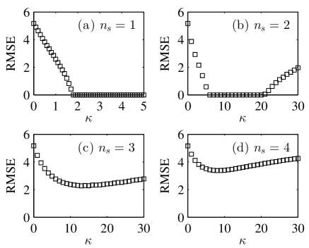
Figure 1: RMSE for different degrees of coupling sparseness $n_{s}=1-4$ from (a) to (d). For $n_{s}=1$ (dense coupling) the RMSE vanishes for $\kappa>\mu\approx 1.75$. For $n_{s}=2$, the RMSE is zero in a certain range of $\kappa$. Finally, for $n_{s}\geq 3$ the observations are too sparse and the RMSE remains positive for all $\kappa$, with an optimal coupling at $\kappa\approx 13$ and $\kappa\approx 8$, for $n_{s}=3$ and $n_{s}=4$, respectively. For each data point, the model was initialized with a random error of order 0.1 at each site.

3 Delay-coordinate nudging

We now propose a modification of the classical nudging scheme in Eq. (2) to incorporate also dynamical information from delayed coordinates. The new DA scheme takes the form

$$\dot{\mathbf{v}}=\tilde{\mathbf{g}}({\mathbf{v}})+\left[\sum_{n=0}^{P-1}\kappa_{n}\mathbf{D}({\mathbf{u}}^{n\tau}-{\mathbf{v}}^{n\tau})\right],$$ (6)

where the superscript $n\tau$ denotes the time interval of delay, such that $\mathbf{v}^{n\tau}\equiv\mathbf{v}(t-n\tau)$, and $P$ is the total number of (present plus delayed) observations used at each observed site. Therefore, in contrast to Eq. (2) the model is now driven not only by the discrepancy with the observations at present time ($n=0$), but also by a finite number of past observations ($n\geq 1$), each of them contributing with an independent coupling strength $\kappa_{n}$.

In the context of dynamical systems theory it is well known that, if some variables of a system cannot be measured, the attractor’s topology can be nonetheless reconstructed using delayed variables, according to the Takens’s delay embedding theorem (Kantz and Schreiber, 1997). This indicates that delayed variables convey useful information that only very recently has been considered for DA purposes (Rey et al., 2014a, b). It is worth noting that the use of delayed coordinates in Eq. (6) does not imply the need for additional observations, but just the storage and use of a finite number of previous measurements. Also note that the delay-coordinate nudging scheme that we introduce in this paper constitutes the simplest method of using the information from past observations and other, more involved, schemes can be envisaged. The increase of computational cost of the new algorithm relative to the standard nudging is negligible, and the new procedure keeps the easiness of implementation that makes the nudging attractive for applications in large-dimensional systems.

Further theoretical justification for the validity of the new delay-coordinate nudging algorithm is postponed to Sec. 6.

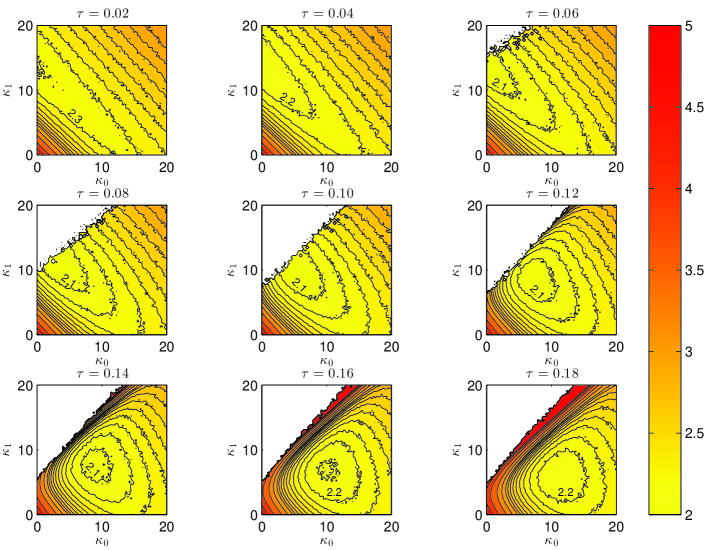
Figure 2: Colour shading depicting the RMSE for $n_{s}=3$ and several delays. In the most yellowish region the RMSE is below $2.1$. In the small RMSE regions, the contour lines are at levels separated by intervals of $0.1$ in RMSE. In several subplots there is a white region in the upper left corner indicating where the algorithm is found to be unstable.

4 Numerical Analysis: Perfect model scenario

We start considering a perfect model scenario, $\tilde{\mathbf{g}}=\mathbf{g}$, and implement delayed nudging in the Lorenz-96 model using only one delayed coordinate at each observation site (i.e. $P=2$). The equation for the model, forced by the nudging terms, reads:

$$\dot{v}_{i} = v_{i-1}\left(v_{i+1}-v_{i-2}\right)-v_{i}+F$$ (7)

$$+ \begin{cases}\kappa_{0}(u_{i}-v_{i})+\kappa_{1}(u_{i}^{\tau}-v_{i}^{\tau})&\mbox{if $i\in{\cal M}$}\\ 0&\mbox{if $i\notin\cal{M}$}\end{cases}$$

Given the results depicted in Figure 1 for the standard nudging without delay, we concentrate the attention on studying the delayed coordinate approach when $n_{s}\geq 3$.

4.1 Case I: $n_{s}=3$

In Figure 2 we present our results for a sparseness $n_{s}=3$, i.e. when observations are available every $3$ sites, so that the subset of observed sites is ${\cal M}=\{1,4,7\ldots\}$. For several values of $\tau\in[0.02,0.2]$, we have varied $\kappa_{0}$ and $\kappa_{1}$ with step-sizes $\Delta k=0.25$.

The standard nudging without delay is recovered in Figure 2 along the $\kappa_{0}$-axis, since for $\kappa_{1}=0$ the delay is irrelevant, and the isolines intercept the axis at the same points in all panels. The lowest RMSE, the clearest yellow in the figure, is in the range $2-2.1$; note that the minimal RMSE without delay is $2.28$ (Sec. 2). The lowest RMSE region appears for $\tau$ as large as $0.06$ and progressively moves away from the $\kappa_{1}$ axis as $\tau$ increases, eventually disappearing for $\tau\geq 0.18$. This behaviour seems to suggest the existence of an optimal delay $\tau$. Also, it shows that, for increasing $\tau$, a larger weight has to be given to the present time observations (increasing $\kappa_{0}$ and decreasing $\kappa_{1}$).

While results show that delay allows to achieve smaller RMSE than in the classic approach with no delay, they also reveal that caution has to be taken when choosing the forcing strength. In fact, delayed nudging becomes unstable in certain regions of the $\kappa_{0}-\kappa_{1}$ plane (see e.g. $\tau=0.06$ in Figure 2). The region of divergence is displayed in white in Figure 2. In agreement with the theoretical argument outlined in Sec. 6, those white regions remain above the bisector $\kappa_{0}=\kappa_{1}$ for all delays, so the choice $\kappa_{0}=\kappa_{1}$ is always safe and free of divergences and, at the same time, it also leads to a significant reduction of the RMSE (provided the value of $\tau$ is not too large).

To better apprehend the significance of Figure 2, we represent in Figure 3 the infimum RMSE achieved as a function of $\tau$: each circle corresponds to an optimal $\tau$-dependent combination of $\kappa_{0}$ and $\kappa_{1}$. For instance the smallest RMSE ($\approx 1.99$), corresponding to the filled circle in Figure 3, is obtained with $\tau_{\mathrm{opt}}=0.08$ for the optimal combination $(\kappa_{0},\kappa_{1})=(3,11.25)$, with the delayed observation coupling strength being almost $4$ times larger than that for the present time observation. In fact, we find numerically that for $\tau\leq 0.07$ the delayed coordinate greatly dominates the optimum coupling. The trade-off option, $\kappa_{0}=\kappa_{1}$, is also displayed (squares) in Figure 3. This simple choice substantially reduces the computational cost associated with the tuning of the relaxation coefficients because the search for the infimum RMSE is restricted to the subspace $\kappa_{0}=\kappa_{1}$. With this choice we achieve a reasonably small RMSE ($\approx 2.04$), at $\tau=0.12$ for $\kappa_{0}=\kappa_{1}=8$, see the filled square in Figure 3. In summary, we numerically find $\inf(\mathrm{RMSE})=1.99$, $2.04$ and $2.28$ for the delay-coordinate nudging with full forcing-delay optimization, delay optimization with the constraint $\kappa_{0}=\kappa_{1}$, and nudging without delay, respectively.

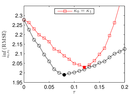
Figure 3: Smallest RMSE achieved with $n_{s}=3$ for each value of $\tau$ (circles). The red squares are the results after restricting to the subspace $\kappa_{0}=\kappa_{1}$ (the bisector of the panels in Figure 2). Note that for $\tau=0$ we recover the optimal RMSE corresponding to the classical (undelayed) case.

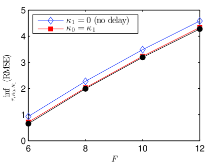
Figure 4: Infimum RMSE over $\tau$, $\kappa_{0}$ and $\kappa_{1}$ achieved for different values of parameter $F$ (filled circles). For comparison, the results restricting to the subspaces without delay (diamonds) and with equal couplings, $\kappa_{0}=\kappa_{1}$ (filled squares) are also represented.

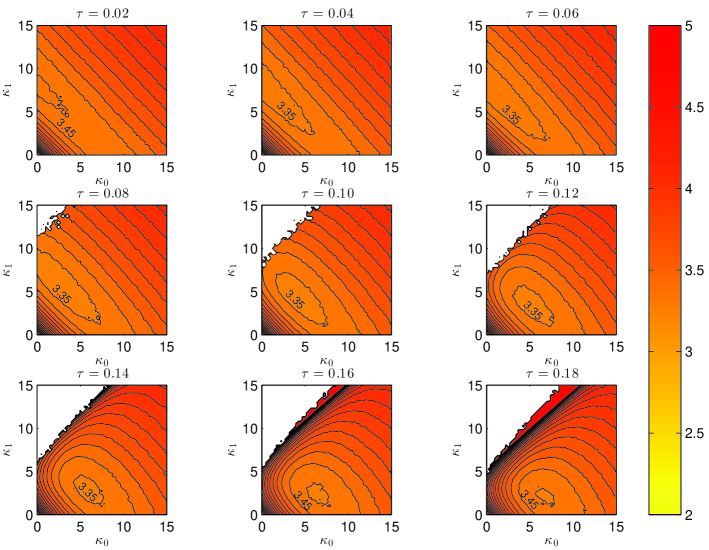
Figure 5: Colour shading depicting the RMSE for $n_{s}=4$ and several delays. The contour lines are at levels separated by intervals of $0.1$ in RMSE. The white region in the upper left corner of some plots indicates where the algorithm is found to be unstable.

As a check for robustness of our numerical analyses, we repeated the simulations presented in Figures 2 and 3 for other values of the external forcing $F$ of the model, finding no qualitative differences in the relative performances of the algorithms. Note that the Lorenz-96 model (3) becomes progressively more chaotic when parameter $F$ is increased: both the number and the magnitude of the positive Lyapunov exponents increase monotonically with $F$. Figure 4 summarizes these results, where we plot with filled circles the infimum RMSE as $\tau$, $\kappa_{0}$ and $\kappa_{1}$ are freely varied for different values of the external forcing $F$. For comparison, the RMSEs obtained when we restrict ourselves to the subspaces $\kappa_{1}=0$ (classical nudging without delay) and $\kappa_{0}=\kappa_{1}$ are also represented with blue diamonds and red squares, respectively. We find that the results systematically improve (lower RMSE) when using delay coordinates. Interestingly, the gain with respect to the standard approach barely depends on the degree of ‘chaoticity’ of the underlying dynamics, i.e. the number of positive Lyapunov exponents, suggesting that delay-coordinate nudging is systematically more effective in controlling the error growth than the classical (nondelayed) nudging. Moreover the choice $\kappa_{0}=\kappa_{1}$ performs also very well, with only minor degradation with respect to the fully optimized case. This is an encouraging result as it suggests that DA can be greatly enhanced by restricting to the $\kappa_{0}=\kappa_{1}$ subspace, without the need of running longer search experiments to determine the optimal values in the full space of couplings $\kappa_{0}$ and $\kappa_{1}$. The optimal parameter values for different values of $F$ are summarized in Table 1.

Table 1: Optimal tunning for different sets of free parameters in the case $n_{s}=3$. The left-most row lists the four different values of $F$ used in Fig. 4.

$F$	$\kappa_{\mathrm{opt}}$ (no delay)	$(\tau,\kappa_{0}=\kappa_{1})_{\mathrm{opt}}$	$(\tau,\kappa_{0},\kappa_{1})_{\mathrm{opt}}$
6	11	$(0.15,6)$	$(0.11,2,9)$
8	13	$(0.12,8)$	$(0.08,3,11.25)$
10	15	$(0.1,9.25)$	$(0.06,1.75,14)$
12	16	$(0.09,9.25)$	$(0.05,1.25,15.75)$

4.2 Case II: $n_{s}=4$

We now increase sparseness by enlarging the distance between adjacent observed sites from $n_{s}=3$ to $n_{s}=4$, so that the total number of observations is now $M=15$ in a system of size $N=60$. This choice makes the DA more challenging, as the state estimation relies now on less observations and the RMSE will tend to grow. The classical nudging without delay achieves an RMSE $\approx 3.37$. Figure 5 is similar to Figure 2, and qualitatively reproduces the pattern found for $n_{s}=3$. Delay-coordinate nudging improves systematically over the standard approach, with the smallest RMSE being $\approx 3.28$ for $\kappa_{0}=1$, $\kappa_{1}=7$ and $\tau=0.06$. Areas of error divergence are present in the upper left portions of the panels, when $\tau\geq 0.08$ and, as observed for the case $n_{s}=3$, the bisector $\kappa_{0}=\kappa_{1}$ represents a choice for the forcing coefficients that prevents error divergence and leads to a minimum RMSE $\approx 3.31$, lower than the standard approach. Note, nevertheless, that the skill gain due to the use of delay-coordinates is smaller for $n_{s}=4$ than that with $n_{s}=3$, see Figure 6. While we achieved improvements of the order of $10\%$ for $n_{s}=3$, the RMSE for $n_{s}=4$ barely decreases a $2.5\%$, with respect to the classical nudging.

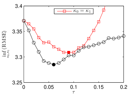
Figure 6: Smallest RMSE achieved with $n_{s}=4$ for each value of $\tau$ (circles). The red squares are the results after restricting to the subspace $\kappa_{0}=\kappa_{1}$ (the bisector of the panels in Figure 5).

4.3 The effect of multiple past observations: $P>2$

We briefly investigate in this section the effect of using more than one delayed observation, i.e. $P>2$ in Eq. (6). This configuration is difficult to study systematically with numerical experiments due to the large number of independent parameters that need to be tuned, $\tau$ and $\kappa_{n=0,\ldots,P-1}$. As a trade-off we decided to simplify the analysis by assuming equal couplings $\kappa_{n}=\kappa/P$, therefore working with two free parameters only, namely, the delay $\tau$ and the aggregate coupling $\kappa$. The infimum RMSE over $\kappa$ as a function of $\tau$ is shown in Figure 7, for three values of $P=2,3,4$ and $n_{s}=3$. Increasing from $P=2$ to $3$ leads to a clear improvement in the assimilation, with the smallest RMSE decreased from $2.043$ to $2.022$. Nevertheless, a further increase to $P=4$ (i.e. $3$ delayed observations) does not yield much gain and, in fact, the improvement seems to saturate. Interestingly, Figure 7 indicates that the optimal total delay does not change significantly in the three experiments, as reflected by an almost complete superposition of the curves with $(P-1)\tau$. In practice, by increasing $P$, the optimal $\tau$ decreases so that the total delay is kept almost constant. This finding is also consistent with the theoretical framework in Sec. 6.

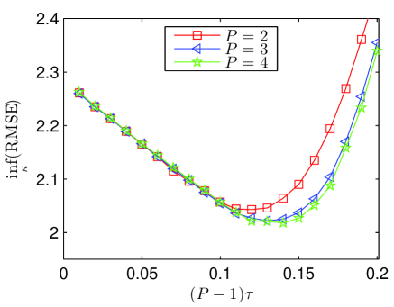
Figure 7: Minimal RMSE for different values of $\tau$ and $P$. The computations are carried out restricting to the subspace with uniform coupling $\kappa_{n}=\kappa/P$, $n=0,\ldots,P-1$.

5 Numerical analysis: imperfect model scenario

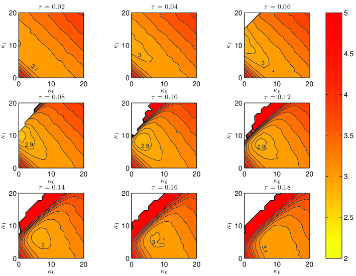
Figure 8: Colour shading depicting the RMSE for $n_{s}=3$ and several delays. The model is governed by Eq. (7) while the truth has more complex dynamics given by Eq. (8). The contour lines are at levels separated by intervals of $0.1$ in RMSE.

In this section, we test the robustness of the delay-coordinate nudging method upon model imperfections. This configuration is closer to realistic contexts where nudging is usually applied. Model error can have, in practice, a number of different origins such as parametric misspecification, numerical discretization or the lack of some process in the description of the reality afforded by the model. We will focus here on the latter case. This is a particularly demanding problem for DA (see e.g. (Mitchell and Carrassi, 2015) and references therein). It is worth to mention here that we have also studied the parametric error case, with a mismatched $F$ in the model, and have obtained equally satisfactory results (not shown).

To this aim, we now assume the truth dynamics includes degrees of freedom, which are absent and not described in the model. Specifically, we adopt the two-scale version of the Lorenz-96 model (Lorenz, 1996) for the truth:

$$\dot{u}_{i}=u_{i-1}(u_{i+1}-u_{i-2})-u_{i}+F-\frac{h\,c}{b}\sum_{j=1}^{J}y_{j,i}$$ (8a)

$$c^{-1}\dot{y}_{j,i}=b\,y_{j+1,i}(y_{j-1,i}-y_{j+2,i})-y_{j,i}+\frac{h}{b}u_{i},$$ (8b)

where the additional $y$ variables are, like $u$ variables, defined on a ring, and thus $y_{J+1,i}=y_{1,i+1}$, $y_{J+2,i}=y_{2,i+1}$, $y_{0,i}=y_{J,i-1}$. The constant $c$ sets the time scale for $y$ variables and we choose $c=10$ in our simulations, so that $y$ evolves $10$ times faster than the (slow) variables $u$. Accordingly, we reduced the time step of our numerical integration by a factor $10$, setting $dt=10^{-4}$ for both the truth, Eq. (8), and the model, Eq. (7). The other parameters are taken as $b=J=F=10$, what implies that the ring of $y_{j,i}$ variables is composed of $N\times J=600$ sites. Parameter $b$ controls the amplitude of the oscillations of $y$, which are ten times smaller than those of the $u$ variable. Moreover parameter $h$, controlling the interaction strength between $u$ and $y$ variables, is set to $h=1$ (which means a strong interaction (Herrera et al., 2011; Pazó et al., 2014)); note that $h=0$ decouples $u$ and $y$ and the perfect model scenario is recovered.

We select $P=2$ in the delay-coordinate nudging scheme and, in order to lower the computational load, we scan the RMSE for parameters $\kappa_{0}$ and $\kappa_{1}$ with larger step sizes, $\Delta\kappa=1$. Results are displayed in Figures 8 and 9 that are the analogue of Figures 2/5 and of Figures 3/6, respectively.

The obvious consequence of model error is to make the overall RMSE level higher than in the perfect model scenario. But, qualitatively, Figure 8 clearly shows similar features than those reported in the perfect model scenario, with the lowest RMSE area departing from the ordinate-axis (i.e. increasing $\kappa_{0}$) for increasing $\tau$. Also in this case we see that the bisector, $\kappa_{0}=\kappa_{1}$, represents viable choice for the forcing terms ensuring better performance than in the classical nudging case with no delay. This is further highlighted in Figure 9 that shows the improvement over the standard approach by using a fully optimized delay coordinates nudging (filled circle) and the case of the minimum RMSE restricted to the bisector line $\kappa_{0}=\kappa_{1}$ (filled square). When compared with the perfect model case, Figure 3, we see now that the curves are much less smooth: small departures from the optimal coupling lead to substantially worse RMSE than the optimized choice. This higher sensitivity of the algorithm to coupling parameter values seems to be a direct outcome of the presence of model error.

The results of Sections 4 and 5 are summarised in Table 2, which shows the infimum RMSE for the standard and delay-coordinate nudging.

Table 2: RMSE for the standard and delay-coordinate (DC in the table) nudging with observations every 3 ($n_{s}=3$) or 4 ($n_{s}=4$) sites and in case of perfect (Perf) or imperfect model (Imp).

Nudging Method	$n_{s}=3$	$n_{s}=3$	$n_{s}=4$
	Perf	Imp	Perf
Standard	2.28	3.05	3.37
DC (optimized)	1.99	2.76	3.28
DC (sub-optimal $\kappa_{0}=\kappa_{1}$)	2.04	2.88	3.31

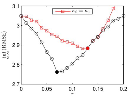
Figure 9: Smallest RMSE achieved with $n_{s}=3$, in the presence of model error, for each value of $\tau$ (circles). The red squares are the results after restricting to the subspace $\kappa_{0}=\kappa_{1}$ (the bisector of the panels in Figure 8).

6 Mathematical discussion on delay-coordinate nudging

In this section we present a heuristic justification of our method for nudging with delay coordinates and of its enhanced skill with respect to standard nudging. Our argumentation leads to an estimation of the order of magnitude of the optimal delay $\tau_{\mathrm{opt}}$ to be used in the algorithm.

Let us begin the discussion by recalling a property that is well known by forecast practitioners: in the nudging implementation one seeks to have the forcing term strong enough to be effective in driving the model toward the observations, but weak enough to avoid dynamical shocks caused by pushing the model to occupy states in the phase-space out of its attractor. As a general rule, nudging has been always implemented so that the forcing term does not exceed the smallest term in the prognostic equation (Hoke and Anthes, 1976). Figure 1(b) exemplifies this effect: even with a perfect model ($\tilde{\mathbf{g}}={\mathbf{g}}$), observational sparseness causes the “synchronization manifold”, $\mathbf{u}=\mathbf{v}$, to become unstable for too large delay-coordinate couplings. And in Figure 1(c) we see how with even sparser observations this trade-off between weak and strong coupling leads to a certain optimal coupling, as complete synchronization between truth and model cannot be attained. With this negative effect of large coupling in mind, one should seek ways of enhancing synchronization at moderate coupling strengths. Precisely, delayed-coupling has been previously highlighted as a source of enhanced synchronizability in contexts such as neural dynamics (Dhamala et al., 2004).

To simplify the illustration of the problem we consider the delay-coordinate nudging scheme in Eq. (6) and assume hereafter to have full coupling, ${\bf D}={\bf I}$, with ${\bf I}$ being the identity matrix in $\mathbb{R}^{N}$. We expect that if stability at moderate-forced coupling is enhanced by delay in this case, then this will translate into a better assimilation when the coupling is not dense (${\bf D}\neq{\bf I}$). This is, admittedly, only a plausible expectation that cannot be further formalized since we do not know how each particular system will respond to coupling sparseness, but we expect it to be true in the general case. Our analysis relies on the study of infinitesimal deviations ${\mathbf{w}}$ off the synchronization manifold, ${\mathbf{v}}={\mathbf{u}}+{\mathbf{w}}$, governed by linear equations. We make a further assumption here since assimilation error is obviously non-infinitesimal and its dynamics nonlinear. In sum, we assume that delay-induced gain in the synchronization stability obtained for (i) infinitesimal error and (ii) dense coupling will yield smaller assimilation error, when the error is not small and the coupling is not dense.

Mathematically, the dynamics of infinitesimal ${\mathbf{w}}$ with dense coupling, ${\bf D}={\bf I}$, is described by the linearisation of (6):

$$\dot{\mathbf{w}}=\mathbf{\partial_{u}}\mathbf{g}({\mathbf{u}})\,{\mathbf{w}}-\kappa_{0}\,{\mathbf{w}}-\kappa_{1}\,{\mathbf{w}}^{\tau}$$ (9)

where $\mathbf{\partial_{u}}{\bf g}({\mathbf{u}})$ is the Jacobian matrix of the dynamics evaluated at the system current state $\mathbf{u}$. In writing Eq. (9), and hereafter, we assume $P=2$ since, as described in previous sections, this case already captures the effect of the delay coordinates; it is then trivial to extend the analysis to larger $P$ if desired.

The stability of synchronization is adequately quantified by the exponential growth rate of $\|{\mathbf{w}}\|$, customarily referred to as the ‘transverse Lyapunov exponent’ (TLE). This is defined as the exponential growth rate of infinitesimal perturbations:

$$\mathrm{TLE}=\lim_{t\to\infty}\frac{1}{t}\ln\|{\mathbf{w}}\|.$$ (10)

If no coupling is present ($\kappa_{0}=\kappa_{1}=0$), the chaotic dynamics of the system elicits an exponential growth of ${\mathbf{w}}$: $\|{\mathbf{w}}(t)\|\simeq\|{\mathbf{w}}(0)\|\exp(\mu t)$, where $\mu$ is the Lyapunov exponent, and trivially $\mathrm{TLE}=\mu$.

If we now let $\kappa_{0}$ and $\kappa_{1}$ to be nonzero, it is tempting to insert the exponential ansatz ${\mathbf{w}}(t)\sim{\mathbf{w}}(0)\exp(\lambda t)$ into (9), and derive the characteristic equation:

$$\lambda=\mu-\kappa_{0}-\kappa_{1}e^{-\lambda\tau}$$ (11)

Unfortunately, this equation does not exactly describe the asymptotic dynamics of $\mathbf{w}$, unless $\mathbf{\partial_{u}g}$ is constant (like occurs if $\bf u$ is a fixed point), due to the subtle interplay between a fluctuating matrix and the delay. Nonetheless, among the spectrum of solutions of Eq. (11), the branch that correspond to the largest real part, denoted here by $\lambda_{d}$, yields an estimation of the TLE. The estimation $Re(\lambda_{d})\approx\mathrm{TLE}$ is exact for $\tau=0$ and progressively deteriorates as $\tau$ increases. In Figure 10 we illustrate with an example (setting $\tau=0.05$ and $\kappa_{0}=\kappa_{1}=\kappa/2$) how the characteristic Eq. (11) estimates the TLE. In the figure we represent with triangles the exact TLE numerically obtained via integration of Eq. (9), and $Re(\lambda_{d})$ —easily obtained after inserting the Lyapunov exponent $\mu\simeq 1.75$ into (11)— is depicted by a solid line. In spite of the evident roughness of the approximation, the crucial point of our reasoning is that for both the true TLE and the approximation $Re(\lambda_{d})$ there is a range of $\kappa$ values where the TLE is smaller with the use of delay-coordinates than without, $\mathrm{TLE}(\tau=0)=\lambda_{d}=\mu-\kappa$. In other words, delay favours the stability of synchronization with respect to the delay-free case; compare the triangles and the small circles in Figure 10.

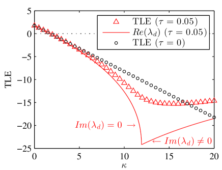
Figure 10: Transverse Lyapunov exponent as a function of $\kappa(=2\kappa_{0}=2\kappa_{1})$ for $\tau=0.05$ (triangles) and $\tau=0$ (circles, $\mathrm{TLE}=\mu-\kappa$). We observe the TLE is smaller with than without delay in the interval $3<\kappa<17$. The solid line is $Re(\lambda_{d})$, where $\lambda_{d}$ is the solution of Eq. (11) with the largest real part.

In view of the cusp in the theoretical continuous line in Figure 10, it is useful to search for a relationship between $\tau$ and the “optimal” value $\kappa_{*}$ where the minimum of $Re(\lambda_{d})$ is located. This relationship is given by the transcendental equation: $\tau=(2/\kappa_{*})\exp[(\mu-\kappa_{*}/2)\tau-1]$. This permits an estimation of the order of magnitude of the optimal delay. In our example with the Lorenz-96 model, given the wide range where the optimal coupling is reasonably expected to be, say $\kappa_{*}\in[2,20]$, the transcendental equation predicts $\tau\in[0.029,0.56]$. This is only an estimation of the order of magnitude of $\tau$, but can be a valuable information as a first guess. Note that the optimal $\tau$ are $0.12$ ($n_{s}=3$) and $0.09$ ($n_{s}=4$) in Figures 3 and 6, respectively.

As a final comment, we resort to Eq. (11) to rationalize why choosing $\kappa_{1}>\kappa_{0}$ may destabilize the nudging algorithm, particularly for non-small delays (the white regions in Figures 2, 5, and 8). Note first that for non-small $\tau$, and unless $\kappa$ is too small, the leading solution, i.e. the one with largest real part, has $Im({\lambda_{d}})\neq 0$ (this branch is, for instance, the solid line at the right of the cusp point in Figure 10). Given our expectation of dominant imaginary eigenvalues in Eq. (11), we may foresee that oscillating modes (with nonzero imaginary part) dominate the fluctuations along the chaotic trajectory when delay is large. The key point is that those modes are associated with certain finite-time exponents $\Lambda=\Lambda_{r}+i\Lambda_{i}$, which leads to a coefficient $e^{-\Lambda_{r}\tau}e^{-i\Lambda_{i}\tau}$ in $\kappa_{1}$, see Eqs. (9) and (11). The source of instability is the factor $e^{-i\Lambda_{i}\tau}$. In the worst situation ($\Lambda_{i}\tau=\pm\pi,\pm 3\pi,\ldots$) the sign of the $\kappa_{1}$ term is flipped, so it becomes a destabilizing contribution. This line of reasoning also suggests that if $\kappa_{0}\geq\kappa_{1}$ the non-delayed part preserves the stability of the nudging algorithm, while choosing $\kappa_{0}<\kappa_{1}$ can not guarantee the stability of the nudging algorithm, specially if the delay is non-small or $\kappa_{1}\gg\kappa_{0}$. This argument is mainly intuitive and heuristic. As such it does not represent a mathematical proof but rather a reasoning of what contributions are expected to affect the stability of the algorithm and guiding the practical implementation of the delay-coordinated nudging.

7 Conclusions

A new approach for DA, the delay-coordinate nudging, has been proposed and extensively investigated. It merges the use of delay coordinates, typical of phase-space reconstruction by temporal embedding, with the standard nudging technique. In the delay-coordinate nudging, both present and past observations are used to nudge the model evolution at each time-step, with negligible increase in computational cost.

Delay-coordinate nudging has been numerically compared with standard nudging in the context of the Lorenz-96 model, for different observational densities, and in the case of both perfect and imperfect model. In all the circumstances considered the new approach permits to achieve a better skill, measured using the RMSE, than that obtained with standard nudging. The number of parameters to be optimized— namely, the coupling coefficients— grows with the number of delay coordinates. However numerical results suggest that: (i) using the same coefficients for all observations already provides a systematic improvement over the classical nudging (only slightly worse than the fully optimized case), and (ii) the performance improvement almost saturates when the number of used delayed observations is larger than $3$. Both facts crucially reduce the optimization cost and open the path for the implementation of delay-coordinate nudging in realistic frameworks.

A connection between the optimal length of the delay, $\tau_{\mathrm{opt}}$, and the dominant Lyapunov exponent of the model dynamics is put forward by studying the stabilization conditions of the synchronization manifold. In the case of using only one delayed observation ($P=2$), the estimate of $\tau_{\mathrm{opt}}$ obtained is consistent with the numerical observations. The same line of reasoning has allowed us to interpret the existence of an unstable regime for the delay-coordinate nudging scheme, observed numerically for certain couplings satisfying $\kappa_{1}>\kappa_{0}$, as arising from oscillating instabilities along the chaotic trajectory. While a formal proof of this relation has not been established, heuristic arguments were provided to support it.

Summarizing, delay-coordinate nudging represents a straightforward amelioration over the standard approach with a small increase of the computational cost. As a continuous data assimilation method, the present approach is also related to recent studies where incomplete data are continuously assimilated to retrieve the signal in fluido-dynamical systems, and that provide an analysis of the temporal and spatial resolution of the observations to achieve a satisfactorily reconstruction of the system’s state (Blomker et al., 2013; Farath et al., 2015). Indeed in these latter works a continuous time 3DVar is adopted implying the use of a spatial extended error covariance matrix so allowing for the propagation of the data forcing to unobserved areas. The extension of the present delay-coordinate formulation in combination with a continuos time 3DVar represents an interesting line of follow-on research. Further improvements, inspired in advanced attractor reconstruction methods for systems with multiple time scales (Pecora et al., 2007), may consist in adopting delayed coordinates unevenly distributed in time. Another relevant direction of research is the combination of delay-coordinate nudging with advanced initialisation methods for coupled models that account for model bias. All in all, the application to more realistic, observational and model, scenarios is a natural direction of prosecution of this study.

We thank Miguel A. Rodríguez for fruitful and interesting discussions. We acknowledge support by MINECO (Spain) under project No. FIS2014-59462-P. DP acknowledges support by MINECO (Spain) under the Ramón y Cajal programme. AC was supported by the EU-FP7 project SANGOMA under grant contract 283580.

References

- Abarbanel et al. (2009) Abarbanel HDI, Creveling DR, Farsian R, Kostuk M. 2009. Dynamical state and parameter estimation. SIAM J. Appl. Dyn. Syst. 8: 1341–1381, 10.1137/090749761.
- Anthes (1974) Anthes RA. 1974. Data assimilation and initialization of hurricane prediction model. J. Atmos. Sci. 31: 702–719.
- Auroux (2009) Auroux D. 2009. The back and forth nudging algorithm applied to a shallow water model: comparison and hybridization with the 4d-var. Int. J. Num. Meth. In Fluids 61: 911–929.
- Auroux and Blum (2008) Auroux D, Blum J. 2008. A nudging-based data assimilation method: the back and forth nudging (bfn) algorithm. Nonlin. Processes Geophys. 15(2): 305–319, 10.5194/npg-15-305-2008.
- Blayo et al. (2014) Blayo E, Bocquet M, Cosme E, Cugliandolo LF. 2014. Advanced Data Assimilation for Geoscience: Lecture Notes of the Les Houches School of Physics. Special Issue, June 2012. Oxford Press: Oxford.
- Blomker et al. (2013) Blomker D, Law K, Stuart A, Zygalakis K. 2013. Accuracy and stability of the continuous-time 3dvar filter for the Navier–Stokes equation. Nonlinearity 26(8): 2193, dx.doi.org/10.1088/0951-7715/26/8/2193.
- Bocquet et al. (2010) Bocquet M, Pires C, Wu L. 2010. Beyond Gaussian Statistical Modeling in Geophysical Data Assimilation. Mon. Wea. Rev. 138(8): 2997–3023, 10.1175/2010MWR3164.1.
- Carrassi et al. (2014) Carrassi A, Weber RJT, Guemas V, Doblas-Reyes FJ, Asif M, Volpi D. 2014. Full-field and anomaly initialization using a low-order climate model: a comparison and proposals for advanced formulations. Nonlin. Processes Geophys. 21(2): 521–537, 10.5194/npg-21-521-2014.
- Dhamala et al. (2004) Dhamala M, Jirsa VK, Ding M. 2004. Enhancement of neural synchrony by time delay. Phys. Rev. Lett. 92: 074 104, 10.1103/PhysRevLett.92.074104.
- Doblas-Reyes et al. (2013) Doblas-Reyes FJ, García-Serrano J, Lienert F, Biescas AP, Rodrigues LRL. 2013. Seasonal climate predictability and forecasting: status and prospects. Wiley Interdisciplinary Reviews: Climate Change 4(4): 245–268, 10.1002/wcc.217.
- Duane et al. (2006) Duane GS, Tribbia JJ, Weiss JB. 2006. Synchronicity in predictive modelling: a new view of data assimilation. Nonlin. Proc. Geophys. 13: 601–612.
- Evensen (2009) Evensen G. 2009. Data Assimilation: The Ensemble Kalman Filter. Springer: New York.
- Farath et al. (2015) Farath A, Jolly M, Titi E. 2015. Continuous data assimilation for the 2d Bénard convection through velocity measurements alone. Physica D 303: 59–66, 10.1016/j.physd.2015.03.011.
- Gelb (1974) Gelb A. 1974. Applied Optimal Estimation. Springer: London.
- Herrera et al. (2011) Herrera S, Pazó D, Fernández J, Rodríguez MA. 2011. The role of large-scale spatial patterns in the chaotic amplification of perturbations in a Lorenz 96 model. Tellus A 63(5): 978–990, 10.1111/j.1600-0870.2011.00545.x.
- Hoke and Anthes (1976) Hoke JE, Anthes RA. 1976. The initialization of numerical models by a dynamic-initialization technique. Mon. Wea. Rev. 104: 1551–1556.
- Houtekamer et al. (2014) Houtekamer P, Deng X, Mitchell H, Baek S, Gagnon N. 2014. Higher Resolution in an Oper- ational Ensemble Kalman Filter. Mon. Wea. Rev. 142: 1143–1162.
- Jazwinski (1970) Jazwinski AH. 1970. Stochastic processes and filtering theory. Academic Press: New York.
- Junge and Parlitz (2001) Junge L, Parlitz U. 2001. Synchronization using dynamic coupling. Phys. Rev. E 64: 055 204, 10.1103/PhysRevE.64.055204.
- Kalman (1960) Kalman R. 1960. A new approach to linear filtering and prediction problems. Trans. ASME, J. Basic Eng. 82: 35–45.
- Kalnay (2002) Kalnay E. 2002. Atmospheric modeling, data assimilation and predictability. Cambridge University Press: Cambridge.
- Kantz and Schreiber (1997) Kantz H, Schreiber T. 1997. Nonlinear time series analysis. Cambridge University Press: Cambridge.
- Lakshmivarahan and Lewis (2013) Lakshmivarahan S, Lewis JM. 2013. Nudging methods: A critical overview. In: Data Assimilation for Atmospheric, Oceanic and Hydrologic Applications (Vol. II), Park SK, Xu L (eds), Springer Berlin Heidelberg, pp. 27–57.
- Lorenz (1996) Lorenz EN. 1996. Predictability - a problem partly solved. In: Proc. Seminar on Predictability Vol. I, Palmer T (ed). ECMWF Seminar, ECMWF: Reading, UK, pp. 1–18.
- Macpherson (1991) Macpherson B. 1991. Dynamic initialization by repeated insertion of data. Q. J. Roy. Meteorol. Soc. 117: 965–991.
- Magnusson et al. (2013) Magnusson L, Alonso-Balmaseda M, Corti S, Molteni F, Stockdale T. 2013. Evaluation of forecast strategies for seasonal and decadal forecasts in presence of systematic model errors. Clim. Dynam. 41: 2393–2409, 10.1007/s00382-012-1599-2.
- Meehl et al. (2013) Meehl GA, Goddard L, Boer G, Burgman R, Branstator G, Cassou C, Corti S, Danabasoglu G, Doblas-Reyes F, Hawkins E, Karspeck A, Kimoto M, Kumar A, Matei D, Mignot J, Msadek R, Navarra A, Pohlmann H, Rienecker M, Rosati T, Schneider E, Smith D, Sutton R, Teng H, van Oldenborgh GJ, Vecchi G, Yeager S. 2013. Decadal climate prediction: An update from the trenches. Bull. Amer. Meteor. Soc. 95(2): 243–267.
- Mitchell and Carrassi (2015) Mitchell L, Carrassi A. 2015. Accounting for model error due to unresolved scales within ensemble Kalman filtering. QJRMS 141: 1417–1428, 10.1002/qj.2451.
- Packard et al. (1980) Packard NH, Crutchfield JP, Farmer JD, Shaw RS. 1980. Geometry from a time series. Phys. Rev. Lett. 45: 712–716, 10.1103/PhysRevLett.45.712.
- Parlitz et al. (2014) Parlitz U, Schumann-Bischoff J, Luther S. 2014. Quantifying uncertainty in state and parameter estimation. Phys. Rev. E 89: 050 902, 10.1103/PhysRevE.89.050902.
- Pazó et al. (2014) Pazó D, López JM, Gallego R, Rodríguez MA. 2014. Synchronizing spatio-temporal chaos with imperfect models: A stochastic surface growth picture. Chaos 24(4): 043115, 10.1063/1.4898385.
- Pazó et al. (2008) Pazó D, Szendro IG, López JM, Rodríguez MA. 2008. Structure of characteristic Lyapunov vectors in spatiotemporal chaos. Phys. Rev. E 78: 016209.
- Pecora et al. (2007) Pecora LM, Moniz L, Nichols J, Carroll TL. 2007. A unified approach to attractor reconstruction. Chaos 17(1): 013110, http://dx.doi.org/10.1063/1.2430294.
- Rabier et al. (2000) Rabier F, Järvinen H, Klinker E, Mahfouf J, Simmons A. 2000. The ECMWF operational implementation of four-dimensional variational assimilation. I: Experiments with simplified physics. Quarterly Journal of the Royal Meteorological Society 126(564): 1143–1170.
- Rey et al. (2014a) Rey D, Eldridge M, Kostuk M, Abarbanel HD, Schumann-Bischoff J, Parlitz U. 2014a. Accurate state and parameter estimation in nonlinear systems with sparse observations. Phys. Lett. A 378(11–12): 869 – 873, http://dx.doi.org/10.1016/j.physleta.2014.01.027.
- Rey et al. (2014b) Rey D, Eldridge M, Morone U, Abarbanel HDI, Parlitz U, Schumann-Bischoff J. 2014b. Using waveform information in nonlinear data assimilation. Phys. Rev. E 90: 062 916, 10.1103/PhysRevE.90.062916.
- Sakov et al. (2012) Sakov P, Counillon F, Bertino L, Lisaeter K, Oke P, Korablev A. 2012. TOPAZ4: an ocean-sea ice data assimilation system for the North Atlantic and Arctic. Ocean Science 8: 633–656, 10.5194/os-8-633-2012.
- Sanchez-Gomez et al. (2015) Sanchez-Gomez E, Cassou C, Ruprich-Robert Y, Fernandez E, Terray L. 2015. Drift dynamics in a coupled model initialized for decadal forecasts. Climate Dynamics : 1–2210.1007/s00382-015-2678-y.
- Sasaki (1970) Sasaki Y. 1970. Some basic formalism in numerical variational analysis. Mon. Wea. Rev. 98: 875–883.
- Servonnat et al. (2015) Servonnat J, Mignot J, Guilyardi E, Swingedouw D, Séférian R, Labetoulle S. 2015. Reconstructing the subsurface ocean decadal variability using surface nudging in a perfect model framework. Climate Dynamics 44(1-2): 315–338, 10.1007/s00382-014-2184-7.
- So et al. (1994) So P, Ott E, Dayawansa WP. 1994. Observing chaos: Deducing and tracking the state of a chaotic system from limited observation. Phys. Rev. E 49: 2650–2660, 10.1103/PhysRevE.49.2650.
- Stauffer and Bao (1993) Stauffer DR, Bao JW. 1993. Optimal determination of nudging coefficients using the adjoint equations. Tellus A 45(5): 358–369, 10.1034/j.1600-0870.1993.t01-4-00003.x.
- Szendro et al. (2009) Szendro IG, Rodríguez MA, López JM. 2009. On the problem of data assimilation by means of synchronization. J. Geophys. Res. 114: D20 109.
- Takens (1981) Takens F. 1981. Detecting strange attractors in turbulence. In: Dynamical Systems and Turbulence, Warwick 1980, Lecture Notes in Mathematics, vol. 898, Rand D, Young LS (eds), Springer Berlin Heidelberg, ISBN 978-3-540-11171-9, pp. 366–381, 10.1007/BFb0091924.
- Vidard et al. (2003) Vidard PA, Le Dimet FX, Piacentini A. 2003. Determination of optimal nudging coefficients. Tellus A 55(1): 1–15, 10.1034/j.1600-0870.2003.201317.x.
- Zou et al. (1992) Zou X, Navon I, Le-Dimet F. 1992. An optimal nudging data assimilation scheme using parameter estimation. Q. J. Roy. Meteorol. Soc. 128: 1163–1186.