Rules in Play: On the Complexity of Routing Tables and Firewalls

Abstract

A fundamental component of networking infrastructure is the policy, used in routing tables and firewalls. Accordingly, there has been extensive study of policies. However, the theory of such policies indicates that the size of the decision tree for a policy is very large ( $O((2n)^{d})$, where the policy has $n$ rules and examines $d$ features of packets). If this was indeed the case, the existing algorithms to detect anomalies, conflicts, and redundancies would not be tractable for practical policies (say, $n=1000$ and $d=10$). In this paper, we clear up this apparent paradox. Using the concept of “rules in play,” we calculate the actual upper bound on the size of the decision tree, and demonstrate how three other factors - narrow fields, singletons, and all-matches - make the problem tractable in practice. We also show how this concept may be used to solve an open problem: pruning a policy to the minimum possible number of rules, without changing its meaning.

I Introduction

Policies, such as routing and filtering policies (implemented in routing tables and firewalls) are essential to the operation of networks. In current, packet-switched networks, routers, switches and middleboxes examine incoming packets, and decide (based on the relevant policy) what course of action to pursue for each packet. Accordingly, fast packet resolution, the operation of checking which rule in the policy is applicable for the packet, is an important area of research. A second important use of policies is in access control lists, for firewalls and intrusion detection; as the security of the system depends on the correctness of such a policy, policy verification is also an important problem. Algorithms for fast operation, design, optimization, and verification of policies work on a decision diagram representation of these policies; a good way to measure the complexity of a policy is the size of its decision diagram.

However, the theory of policy decison diagrams comes with a major caveat. The best known bound for the size of such a diagram is very large - specifically, $(2n-1)^{d}$, where the policy has $n$ rules and the number of features of interest (which we call ’fields’) is $d$. As $n$ is of the order of thousands of rules, and $d$ can easily be $5-10$, it would seem that the complexity of these algorithms is too large for practical cases. But this is not the case at all - in fact, these algorithms are in common use to analyze policies and entire networks [1]!

This paper solves this apparent paradox. We deepen the theory of policy decision diagrams with the idea of keeping track of “rules in play,” which allows us to determine a tight upper bound on the size of a decision diagram and show why the size does not explode for practical policies. We also suggest how this allows us to optimize policies, and obtain truly minimum (rather than just minimal, i.e. with no redundant rules) policies.

We begin by providing our definitions and concepts, in the next section. Next, we discuss decision diagrams and the algorithm to create them, as well as how we modify it to keep track of rules in play. After this, we demonstrate how there are mitigating factors - narrow fields, singletons, and all-matches - that reduce the size of decision diagrams in practice. Finally, we provide our experimental results, discuss how our paper fits into the context of related work, and finish with some concluding remarks.

II Terms and Concepts

In this section, we define the terms and concepts used in the paper, such as policies and properties, and formally introduce our concepts of oneprob, allprob, and fieldwidth. We will introduce decision diagrams and “rules-in-play” in the next section.

II-A Packets, Rules, and Matching

In our work, we model a packet as a $d$-tuple of non-negative integers. Why this model? In order to decide what to do with a packet (whether to forward it, which interface to forward it on, etc.), routers and firewalls examine its various attributes - usually values in the packet header, such as source address, destination address, source port, destination port, protocol, and so on. (In ‘deep packet inspection’, attributes from the packet payload are also checked.) The $d$ fields of our packet model represent the $d$ features examined.

A rule represents a single rule in a flow table. It consists of two parts: a predicate and a decision.

The rule predicate is of the form

$$x_{1}\in[x_{1,1},x_{1,2}]\land x_{2}\in[x_{2,1},x_{2,2}]\ldots x_{d}\in[x_{d,1},x_{d,2}]$$

where each interval $[x_{k,1},x_{k,2}]$ is an interval of non negative integers, drawn from the domain of field $k$. (For example, suppose the third field in packets and rules represents source IP address. In IPv4, the domain of this field is $[0,2^{32}-1]$. Then, in any rule, $0\leq x_{3,1}\leq x_{3,2}\leq 2^{32}-1$.)

The decision is an action, such as (in a firewall) accept or discard. [We call a rule with decision accept an “$accept$ rule”, and a rule with decision discard a “$discard$ rule”.]

A packet that satisfies the predicate of a rule is said to match the rule. For example, the packet $(1,26,7)$ clearly matches the rule

$$x_{1}\in[0,108]\land x_{2}\in[21,65535]\land x_{3}\in[7,616]\to accept$$

II-B Policies and Packet Resolution

A policy consists of multiple rules (as defined in the previous subsection), and a specification of which action to execute, in the event that multiple rules match a given packet. There are two principal methods in use to decide the precedence of matching rules.

1. First Match. The rules are arranged in sequence in the policy, and the action of the first rule in the sequence that is matched by a packet is the action executed.

   This is the method usually used in firewalls.

2. Best Match. One specific field is chosen and, out of the rules matched by the packet, the one with the smallest interval for this particular field has precedence.

   This is the method used in routing tables. The field chosen is the destination IP, and this technique is called ’longest prefix matching’. (In routing tables, IP address intervals are usually denoted by prefixes, e.g., $100.150.200.0-100.150.200.255$, which is really the interval $[1687603200,1687603455]$, is written $100.150.200.0/24$. Thus the best match is by the rule which had the longest prefix out of the rules matched by the packet.)

The practical order of deciding precedence in a router is quite complicated. In short,

1. First, find the best match.

2. In case of conflict, choose rules in the order:

   1. Static routes

   2. Dynamic routes, in order
      (usually EIGRP, OSPF, ISIS, RIP)

   3. Default route

3. If no rule matches, discard the packet.

However, this entire procedure can be effectively reduced to first match, simply by ordering the rules! (The primary sort key in this ordering is the specified prefix length, and the secondary sort key, the type of rule.) Hence, in our work, we assume first match semantics for policies.

The ‘winning’ rule, the decision of which is implemented for a packet, is said to resolve the packet.

II-C OneProb, AllProb, and FieldWidth

In policy research, the complexity of a policy is considered to be affected by two principal factors. The first is $n$, the number of rules in the policy, which can be up to several thousand; the other is $d$, the number of fields in a rule, which is usually around $5-10$. For example, the complexity of the simple standard algorithm for resolution - check, for each of $d$ fields of the packet, that the value falls in the interval specified by the rule; repeat until a rule is matched - is clearly $O(nd)$.

However, we contend that this is not sufficient information to predict the complexity of a policy. There are two other metrics of interest.

The first observation is that, in practice, rules are almost always targeted to very specific uses; as a result, many of their fields are set to either a single specific value, or to “All” - i.e. the entire domain of the field. (For example, firewalls built using Structured Firewall Design[2] have many fields set to All.) As demonstrated in earlier work[3], policies where high proportions of fields are set to single values, or to All, show significantly different behavior than other policies with the same values of $n$ and $d$. To capture this, we use the metrics $allprob$ and $oneprob$.

$allprob$ is the probability that, on randomly choosing a field and a rule in the policy, the interval specified by the rule for the field is “All”.

$oneprob$ is the probability that the interval specified by a randomly chosen rule for a randomly chosen field, is a single value, such as $[6,6]$.

The second observation is that the domains of different fields are of very different sizes. For example, IPv4 addresses take $32$ bits, protocol takes $8$ bits, and version takes $4$ bits in a standard header. We use the metric of $fieldwidth$ to measure narrow fields (whose domain is expressed in a small number of bits); it is the total number of bits needed to express all narrow fields in the policy. The reason for introducing a new metric is that narrow and wide fields have different effects on the complexity of a policy. We provide details in Section V.

III Decision Diagrams

In this section, we describe how policies can be represented using Decision Diagrams, as proposed by Gouda [2].

A decision diagram (over fields $f_{1}..f_{d}$) is an acyclic, rooted digraph. Every terminal node, i.e. one with no outgoing edges, is marked with a decision (for example, in case of firewalls, decisions are accept or discard). Every non-terminal node is marked with the name of a field, and has outgoing edges marked with an interval of values for its field; values marked on the edges from a node do not overlap.

There is at least one directed path from the root to every other node, and no directed path has more than one node labeled with the same field. Thus, a decision diagram represents a simple deterministic finite automaton. Given any packet $p=(p.f_{1},..p.f_{d})$, there is exactly one path from the root corresponding to the field values of $p$, and it terminates in a terminal node; the decision at this node is the decision of the policy for $p$.

We consider the decision diagram in its fully expanded form, as a tree. In our example, the root is labeled $f_{1}$, its children are $f_{2}$, down to $f_{d}$, whose children are the leaf i.e. terminal nodes.

To resolve a packet, we follow a path from the root down to a leaf node, at each node choosing the edge matched by the packet - i.e., labeled with the interval containing the value of the corresponding field for the packet. Given a policy with $n$ rules of $d$ fields, a decision diagram performs packet resolution in $O(d)$ time. Policy verification has the same time complexity as the size of the diagram. (It is essential to check the decision corresponding to packets that match the property; in the worst case , the property specifies all possible packets, and it is necessary to check paths from the root to every terminal node.)

We now extend the algorithm to construct decision diagrams, by introducing the concept of rules in play. A rule $R$ of a policy is “in play” at a node if at least one packet matching $R$ follows a path through the node when it is resolved. $R$ is in play at an edge if it is in play at the node into which the edge leads. Annotating the nodes with the rules in play requires only slight modification to the algorithm for building a decision diagram; we present the algorithm in Figure 1. In Figure 2, we show an example, building an annotated decision diagram from the policy

$$x\in[10,110]\land y\in[90,190]\to 0$$

$$x\in[20,120]\land y\in[80,180]\to 1$$

For our first demonstration of how rules in play can be useful, we demonstrate how, given a policy, we can use the rules in play at the leaf nodes, and find a $minimum$ equivalent policy (equivalent policies have the same decision for every packet). We delete rules, without changing the decision of the policy for the packets reaching any leaf node. (As we are not adding rules, there will be no new paths or new leaves to consider.)

Consider a leaf node with the $accept$ rules $3,13$ and the $discard$ rule $7$ in play. So long as rule $3$ remains, deleting other rules does not affect the decision at this leaf. What if we delete rule $3$? We must delete rule $7$ (so it does not become the first rule to match these packets), and keep rule $13$. Using $x_{i}$ to mean that rule $i$ is present, we must satisfy

$$x_{3}\lor(\lnot x_{7}\land(x_{13}))$$

We can apply this logic recursively: if we had $accept$ rules $3$, $13$ and $23$, and $discard$ rules $7$, $10$ and $17$, then

$$x_{3}\lor(\lnot x_{7}\land(\lnot x_{10}\land(x_{13}\lor(\lnot x_{17}\land(x_{23})))))$$

must be satisfied, to preserve the policy decision at this leaf.

1. At a leaf node, we start with the first rule in play. All other rules with the same decision are complying rules, and the others are conflicting rules.

2. We traverse the list of rules in play, in order, building an expression (string).

3. If the rule $R_{i}$ is complying, we add “$x_{i}\lor($”. If it is conflicting, we add “$\lnot x_{i}\land($”.

4. At the end, we close all parentheses.

Taking the AND of the expressions for all the leaf nodes, we get an expression which must be satisfied to keep the decision of the policy unchanged for all packets.

To find the minimum policy, we create our expression for the original policy (as described above), and search for the solution with the smallest number of $x_{i}$ set to $1$ - a Min-One SAT problem. This gives us the smallest combination of the rules in the policy that preserve its semantics for all packets, a minimum policy (rather than the minimal policies obtained by trimming as many redundant rules as possible). So far, this algorithm is too slow to be practical for policies of more than $50$ rules; however, we expect optimizing the solver will make it fast enough for real use. We will develop this further in future work.

In the next two sections, we show how, by keeping track of rules in play, we can prove that decision diagrams do not grow exponentially large in practice.

Figure 1: Building annotated decision diagram from policy

procedure AddnewRule(Rule $R$, name $R.name$, node $x$)

    Add $R.name$ to list of rules in play at $x$

    if $x$ is a terminal node then

         Label $x$ with the decision of $R$.

    else

         $i$ is the field of node $x$.

         $R.i$ is the interval for field $i$ in $R$.

         $x.i_{1},x.i_{2}..$ are the values on the edges from node $x$.

         Build new paths from $x$, starting with new outgoing edges labeled with the intervals in $R.i-\{x.i_{1},x.i_{2}..\}$. $\triangleright$ To each edge, add new nodes and edge labels as per remaining fields in $R$. The terminal node has decision of $R$. These nodes start with only one rule in play, i.e. $R.name$.

         for all labels $x.i_{k}$ do

             if $x.i_{k}\cap R.i$ is empty then

                 continue

             else

                 $y$ is the target of edge labeled $x.i_{k}$.

                 for every interval $x.i_{new}\in x.i_{k}-R.i$ do

                     Copy (subgraph rooted at $y$ ).

                     $y^{\prime}$ is the new copy of $y$ itself.

                     Add edge $x\to y^{\prime}$, labeled $x.i_{new}$.

                 end for

                 Relabel edge $x\to y$ with $x.i_{k}\cap R.i$.

                 $AddNewRule(R,R.name,y)$

             end if

         end for

    end if

end procedure

procedure BuildDDiagram(Policy $\{R_{1},R_{2}..R_{n}\}$)

    Create empty node $x$ with no outgoing edges.

    Label $x$ with desired field for root.

    for $index\leftarrow n...1,$ step $-1$ do

         $AddNewRule(R_{index},index,x)$

    end for

    return Decision Diagram rooted at $x$.

end procedure

Figure 2: Example: building a decision diagram, step by step.

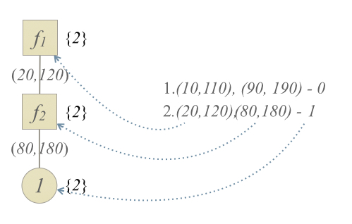
(a)

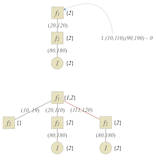
(b)

Step $1$. First rule from bottom, i.e. rule $2$

(c)

Step $2$. Adding $f_{1}$ from next rule, rule $1$.

(d)

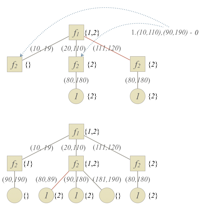
(e)

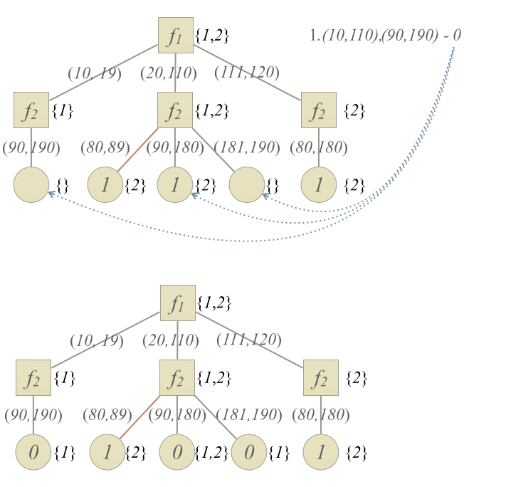
(f)

Step $3$. Adding $f_{2}$ from rule $1$.

(g)

Step $4$. Adding decision from rule $1$.

(h)

IV The Size of Decision Diagrams

In this section, we determine the worst case size of a policy decision diagram, measured as the number of leaf nodes of the diagram. We begin with the existing upper bound.

The intuition behind the bound is that, as the decision diagram is a tree of fixed depth, its size can be maximized by making the branching factor of each node as large as possible.

As there are $n$ rules in the policy, there can be a maximum of $2n-1$ outgoing edges for a node. (Each edge must be labeled with at least one interval. The $n$ rules have $2n$ end points - each interval has a start and an end. These $2n$ end points thus divide the domain into a maximum of $2n-1$ intervals. Hence we can have at most $2n-1$ edges from a node.)

Thus, an upper bound on the size of the decision diagram for a policy of $n$ rules and $d$ fields is $(2n-1)^{d}$.

Our construction, which is mindful of rules in play, allows us to tighten this bound considerably. The intuition behind this is that, while a node with $n$ rules in play can indeed have a branching factor of $(2n-1)$, as seen above, not all these branches still have $n$ rules in play! In fact, of the outgoing edges, exactly one edge still has all $n$ rules in play (the one corresponding to the intersection of all the rules). There are also edges with $n-1$ rules in play, $n-2$ rules in play, and so on, down to edges with $1$ rule in play. In our example from Figure 2, consider the edges emerging from the root: edge $(10,19)$ has only one rule in play (the first), edge $(20,110)$ has both rules in play, and edge $(111,120)$ has only one rule in play (the second).

So, in order to construct the largest decision diagram, there are two factors to maximize:

1. The number of branches, i.e. the branching factor at each node

2. The number of rules in play along each branch.

In fact, in the largest possible decision diagram for a given $n$ and $d$, the pattern is that one outgoing edge has $n$ rules in play, two have $n-1$, two have $n-2$, and so on, down to the last two edges which have a single rule in play. This is a dynamic programming problem: given the largest decision diagrams that can be built with $1,2...n$ rules in play, at a depth $d-1$, we can compute the size of the largest decision diagram with depth $d$, and $n$ rules in play. We also have the following observations.

1. For any $d$, when $n=1$, the number of leaves is $1$. (Only a single rule is in play, so there is no branching.)

2. $d=0$ indicates we are at a leaf node, so the size is $1$.

3. When $d=1$, and the number of rules in play is $n$, then the size of the decision diagram (measured by number of leaves) is $2n-1$.

Stating this result formally,

Theorem 1.

If we represent the maximum size (measured by number of leaf nodes) of a decision diagram with $n$ rules and $d$ fields as $f(n,d)$,

$$f(n,d) =2\sum\limits_{i=1}^{n-1}f(i,d-1)+f(n,d-1)$$

for $$n>1,d>1$$

$$f(n,1) =2n-1$$

$$f(1,d) =1$$

Next, we need to prove that this intuitively appealing construction ( all $n$ rules overlapping for one central edge, and rules “falling off” one by one to either side) is in fact the largest possible decision diagram for a given $n$ and $d$. Our proof is as follows.

Consider any decision diagram. It forms a tree, in which every non-leaf node represents a field. Every edge is labeled with an interval (of values for the field represented by the node it starts from), and associated with a list of rules in play at that edge.

We consider how, in constructing the old bound, we maximize the branching factor at a node. Every rule $R_{i}$ has a range $[start_{i},end_{i}]$; these end points ($start_{i}$ and $end_{i}$) segment the domain space into intervals. $n$ rules introduce $2n$ end points, and each point added has the potential to create a new edge. (The set of rules in play is different before and after an end point.) To maximize the number of edges, we assume that no two end points coincide; this gives us $2n-1$ as the number of outgoing edges from a node.

Now, we extend this argument. We will abuse the variable names $n$ and $d$. In general, we now use $n$ to mean the number of rules in play at a node (or an edge) ; the original meaning of $n$, the number of rules in the policy, is the $n$ seen at the root. Similarly, we use $d$ to mean the depth of the subtree rooted at a node; the original meaning of $d$, the number of fields, is the $d$ seen at the root. Clearly, $f(n,d)$ increases monotonically with $n$ and with $d$.

Let us arrange the outgoing edges from a node in ascending order of the values of their labels (intervals). [As these intervals are non overlapping, we can sort them by their start, i.e. smallest values, or by end, i.e. largest values - the order will be the same.] Two edges are said to be adjacent if there exists no edge whose label (interval) lies in between their labels.

Lemma.

In the largest decision diagram for a given $n$ and $d$, the sets of rules in play on adjacent edges differ by one rule exactly.

Proof. Let the rulesets on two adjacent edges be $A$ and $B$.

Let $A=X+Y$ and $B=Y+Z$.

If $X$ and $Z$ are both non-null, then by increasing the $end_{i}$ of rules in $X$, by $1$ (or reducing the $start_{i}$ of rules in $Y$, by $1$) we can add a new edge with the ruleset $X+Y+Z$ in between these edges.

This edge could not already exist. (Let the field be named $f_{1}$. Without loss of generality, assume $f_{1}$ increases going from $A$ to $B$. The labels of rules are intervals - they start once and stop once exactly. $X$ appears on no edge with greater $f_{1}$ than edge labeled $A$, and $Z$ on no edge with less $f_{1}$ than edge labeled $B$. So the edge with $X+Y+Z$ could not have been at some other position.)

Also, adding this edge does not affect the rest of the diagram (for $f_{1}$, the other edges have different values, and are not affected; the other fields are not touched at all). Adding this new edge clearly increases the decision diagram size. But this is the largest decision diagram for this $n$ and $d$, so we have a contradiction.

Now, we have proved that either $X$ or $Z$ is the null set. Without loss of generality, let us assume that $X$ was null.

Can $Z$ also be a null set? This is not possible, because then $A==B$! The edges labelled $A$ and $B$ would be merged to form a single edge.

On the other hand, can $Z$ contain more than $1$ rule?

In this case, $Z=Z_{1}+Z_{2}$, where $Z_{1}$ has one rule and $Z_{2}$ is non-empty. The $start_{i}$ of rules in $Z_{1}$ and $Z_{2}$ coincide.

If we had a decision diagram where all else is the same, but these rules did not share the same $start_{i}$, we would have an extra edge labeled with $Y+Z_{1}$ between these two edges. But this is the largest possible decision diagram for given $n$ and $d$, so again we have a contradiction.

Hence, one of $A-B$ or $B-A$ is the null set, and the other has exactly one rule. This suffices to prove our lemma. ∎

Next, we consider the first edge (i.e. the one with the smallest $start_{i}$. This edge has only one rule in play; if it had more, by a similar construction as above, we could add a preceding edge. Now the next edge can have at most two rules in play, and if we continue to count up, we eventually reach $n$ rules in play. After we reach $n$ rules, on the next edge we can only have $n-1$ rules in play, and so on.

To complete our proof that the largest decision diagram indeed follows this structure, we introduce the idea of “closed” rules. At every edge, besides the number of rules in play, we can keep count of $n^{\prime}$, the number of rules for which we have already exceeded the $end_{i}$. These rules can therefore not come into play at a later edge - they are used up. In our running example, consider the last edge $[111,120]$ coming out of the root; this edge has the second rule in play, and the first rule closed.

Suppose we characterize decision diagrams, for a given $n$ and $d$, by drawing a plot, showing the number of rules in play on an edge vs. the position of the edge (first edge is the one with smallest $start_{i}$, etc.) We know that, for the largest decision diagram, adjacent $y$-values differ by exactly $1$. Given the monotonic nature of $f$, clearly, if the figure for decision diagram $D1$ is enclosed within the figure for another decision diagram $D2$, then $D2$ is larger than $D1$.

Our construction produces a symmetric triangle sloping from $1$ up to $n$ and from $n$ back down to $1$. It is easy to see that, for the rising half, the plot for the largest decision diagram is contained within this triangle; it increases the number of rules in play as quickly as possible. However, it is not so obvious that this condition also holds for the second (falling) half (because our construction also grows the number of closed rules as slowly as possible). Could there be a larger decision diagram whose plot “breaks out” from the triangle? The two plots must intersect, so suppose it intersects the falling half after $k_{o}$ rules have been brought into play and $k_{c}$ rules have been closed,

$$k_{o}+k_{c}=k$$

$$k_{o}-k_{c}=2n-k$$

$$k_{c}\leq k_{o}\leq n$$

which reduces to $k_{o}=n,k_{c}=0$, i.e. the only plot that satisfies the given constraints is our original construction.

This concludes our proof that the largest decision diagram for a given $n$ and $d$ indeed follows the pattern where edges have $1,2...n-1,n,n-1,...2,1$ rules in play. Our bound is tight: the following policy has exactly this decision diagram, and hence, matches the size of this upper bound.

$$x_{1}\in[1,2n-1]\land...\land x_{d}\in[1,2n-1]\to accept$$

$$x_{1}\in[2,2n-2]\land...\land x_{d}\in[2,2n-2]\to discard$$

$$...$$

$$x_{1}\in[n,n]\land...x_{d}\in[n,n]\to discard$$

V Size in real Decision Diagrams

In the previous section, we present our new bound for the size of decision diagrams. This bound is much smaller than the old bound of $(2n-1)^{d}$; for example, for $n=1000$ and $d=10$,

$$f(n,d)=2.808\times 10^{26}<<(2n-1)^{d}=1.019\times 10^{33}$$

. However, this bound, though tight, is still quite large. In this section, we answer the question of why, in practice, decision diagrams do not grow intractably large. The answer makes use of our concepts of oneprob, allprob, and narrow fields.

V-A OneProb and Singletons

In constructing a decision diagram, we have two main operations that increase its size. One is adding a new path; this happens when the new rule specifies new values for a field, i.e. values for which no outgoing edges exist. The other operation is when the interval specified by the rule only partly overlaps with the label of an edge; in this case, we ‘split’ the edge and make copies of the subgraph below. (In our example, the rule has $x\in[10,110]$ and the old edge has $x\in[20,120]$. As they partially overlap, we get new edges labeled $x\in[10,19]$, $x\in[20,110]$, and $x\in[111,120]$.)

Now we consider the impact of singletons. A rule is called a singleton for field $x$ if matches only packets with one single value of $x$, i.e. its interval for $x$ is a single value like $[29,29]$.

Clearly, singletons cannot have partial overlap with any other rule. As a consequence, an edge (from a node labeled $x$) with a singleton (for $x$) cannot be split! This leads immediately to the observation that if all the rules are singletons, the maximum branching factor at a node is not $2n-1$, but $n$ (when all the singletons have different values for $x$, and thus produce different branches). However, this attractive idea is limited in its power: as soon as we introduce a single non-singleton rule $R^{\prime}$, we are back to $2n-1$. [The worst case is when all $n-1$ singletons split $R^{\prime}$, cutting up its interval into $n-1+1=n$ parts in between them. Now we have $n-1$ edges with two rules in play ($R^{\prime}$ and one of the singletons), and $n$ edges with only $R^{\prime}$ in play, so $2n-1$ edges in all. For example, consider rules with intervals $[1,10]$, $[3,3]$ and $[7,7]$; we have $2\times 3-1=5$ edges, labeled with $[1,2]$, $[3,3]$, $[4,6]$, $[7,7]$, and $[8,10]$. ]

To make a stronger argument, we consider the number of rules in play along an edge.

When we have mutliple singletons for a field, there are two choices. They either overlap completely, or they do not overlap at all. If they do not overlap, this increases the branching factor at the node (more outgoing edges). But this means the number of rules in play along those edges (and therefore, at the nodes the next layer down) is reduced! For the largest decision diagram, we need to trade off the “immediate” branching factor at the node and the “potential” for more branching at lower levels. The solution is only obvious at nodes where $d=1$, as the only lower level is the leaf nodes (i.e. no more branching is possible at lower levels); in the largest decision diagram, all singletons of the field where $d=1$ have distinct values.

Singletons increase the size of the decision diagram most effectively if they intersect the interval with the largest possible number of rules in play. Consider the diagram made with the non-singleton rules; the edges follow the standard pattern, with $1,2...n,n-1,...1$ rules in play. Now we introduce a singleton. If it splits an edge with $r$ rules in play, we replace one edge with $x$ rules with two edges with $r$ rules (before and after the singleton), plus one edge with $r+1$ rules (where the $r$ rules and the singleton overlap). If on the other hand, the singleton did not split any edge, it would introduce only one new edge with a single rule in play (the singleton). Clearly, the maximum is when $r=n$.

How are we to proceed when introducing more singletons? This is not straightforward. Let us assume that the number of singletons is $s$, the number of non singletons is $t$, and the depth of the tree (below the node we are considering) is, as usual, $d$. Then to find the size of the largest decision diagram, we try all the partitions of $s$ singletons; for example, if $s=4$, we need to try $1+1+1+1,1+2+1,1+3,2+2$, and $4$. Then, using $g(s+t,d)$ as the formula for maximum size, and $a$ as the number of pieces in the partition $\{s_{1},s_{2},...s_{a}\}$,

$$g(n,d)= 2\sum\limits_{i=1}^{t-1}f(i,d-1)$$

$$+max\Big{[}(a+1)g(t,d-1)$$

$$+\sum\limits_{j=1}^{a}g(t+s_{j},d-1)\Big{]}$$

$$n= s+t$$

where the max is taken over all partitions.

There is a small gap in this argument, which we now explain. How do we know the largest decision diagram is produced by adding singletons to the largest diagram without singletons? The reason is the monotonicity of the size function. With or without singletons, a diagram with more edges and more rules in play along an edge is larger. [It is also of interest to note that a rule being a singleton for one field does not mean it is a singleton for the fields at lower levels! Counted as a rule in play, it is just as powerful as any other rule.] The largest diagram to begin with, also produces the largest increases: other structures also grow fastest by adding singletons that split the edge with the most rules in play, and they cannot have edges with more than $t$ rules in play. For example, consider two diagrams with the number of rules-in-play, $(1,2,1,2,1)$ and $(1,2,3,2,1)$. If we now add two singletons, the first will yield a diagram with the maximum size

$$3g(1,d)+g(2,d)+max\big{(}g(4,d)+2g(2,d),2g(3,d)+3g(2,d)\big{)}$$

and the second,

$$2g(1,d)+2g(2,d)+max\big{(}g(5,d)+2g(3,d),2g(4,d)+3g(3,d)\big{)}$$

which is clearly larger.

The probability that a rule is a singleton is given by $oneprob$, so our intuition is that a high value of $oneprob$ leads to a smaller decision diagram. One point that we have not highlighted, is that singletons are also much less likely to overlap than other rules are; as our focus is on the worst case, we could not make use of this factor, but it most likely also plays a role in the tractable size of practical decision diagrams.

V-B AllProb and All-Matches

The behavior of all-matches, that is, rules that match all values for a given field, is much less complicated. At a given node, there is no choice about where to place the all-matches; they cover the entire domain for the field. So the all-matches all behave like one single large rule, which adds $u$ (the number of all-match rules) to the number of rules in play on each edge. We can update the formula for largest decision diagram as follows.

$$g(n,d)= 2\sum\limits_{i=0}^{t-1}f(i+u,d-1)$$

$$+max\Big{[}(a+1)g(t+u,d-1)$$

$$+\sum\limits_{j=1}^{a}g(t+s_{j}+u,d-1)\Big{]}$$

$$n= s+t+u$$

where, again, $a$ is the number of pieces the singletons are partitioned into, and the max is taken over all such partitions.

The probability that a rule is an all-match is given by $allprob$. An intuitive way to explain of the effect of all-matches is that, when $allprob$ grows sufficiently large, as most of the rules have total (rather than partial) overlap, the size of the decision diagram is reduced. In fact, in the extreme case of $allprob=100$, the decision diagram is a linked list (from the root to the decision of the first rule, which resolves all packets).

V-C Narrow Fields

Our construction of decision diagrams follows an implicit assumption. When we state that the outgoing edges from a node can carve the domain into $2n-1$ pieces, etc., we assume that the domain is large enough to divide into so many distinct pieces.

However, this assumption is not true for some domains. These are the ones we call narrow fields.

Clearly, if a field is represented with $w$ bits, the greatest possible number of outgoing edges is upper bounded by $2^{w}$. [Every possible value of the field labels a distinct edge.] We can extend this argument by placing all the narrow fields together, as the fields closest to the leaves (i.e. with $d=1,2...d_{narrow}$. Suppose $fieldwidth=W$ bits, i.e. the narrow fields can all be represented using $W$ bits. Our computation for the size of the decision diagram does not change for the non-narrow fields; however, the “leaf” nodes for this tree are now the roots of decision trees for the narrow fields, which expand to $2^{W}$ bits each. So we can simply compute the size for the non-narrow bits, and multiply the result by $2^{W}$ to get an upper bound on the size. This idea is similar to the automata size bound of Erradi [4].

$$g(n,d)= 2\sum\limits_{i=0}^{t-1}f(i+u,d-1)$$

$$+max\Big{[}(a+1)g(t+u,d-1)$$

$$+\sum\limits_{j=1}^{a}g(t+s_{j}+u,d-1)\Big{]}$$

$$n= s+t+u$$

for $d>d_{narrow}$, the number of narrow fields, and

$$g(n,d)= g(n,d-1)*2^{w_{d}}$$

otherwise. ($w_{d}$ = bit width of field at height $d$.)

However, this is no longer a strict upper bound. The reason is that, if we do organize the decision diagram with wide fields closer to the root and narrow fields closer to the leaves, some of the edges from the upper nodes to the lower nodes have a very small number of rules in play - $1$, $2$ etc. Clearly, for these edges, the lower nodes are no longer “narrow” fields, as the bound of $2n-1$ is again smaller than $2^{w}$.

Though this bound is no longer tight, in the presence of narrow fields, it also serves to reduce the size of the decision diagram considerably. We present our experimental results in the next section.

VI Results

This section describes our experimental verification of the size bounds for decision diagrams. In Figure 3, we demonstrate the effect of the mitigating factors, on practical policies with $n=100,200...1000$ rules and $d=5$ fields. We show that the effect of the factors compounds together, by showing the original bound $f(n,d)$, then $g(n,d)$, the bound in presence of these factors, introducing first $allprob$, then narrow fields, and finally $oneprob$.

As the maximum size in the presence of singletons requires us to compute and check all partitions - an exponential number - we do not compute the bound for such large $n$; we provide the impact of $oneprob$ for $n=10,20...100$. [The other plots were similar in shape for $n=10,20...100$ and $n=100,200...1000$.] We also checked that these bounds are in fact correct by generating decision diagrams for a large number of policies (a total of approx. two million); the bounds were never exceeded.

Figure 3: Performance of size bounds for Decision Diagrams

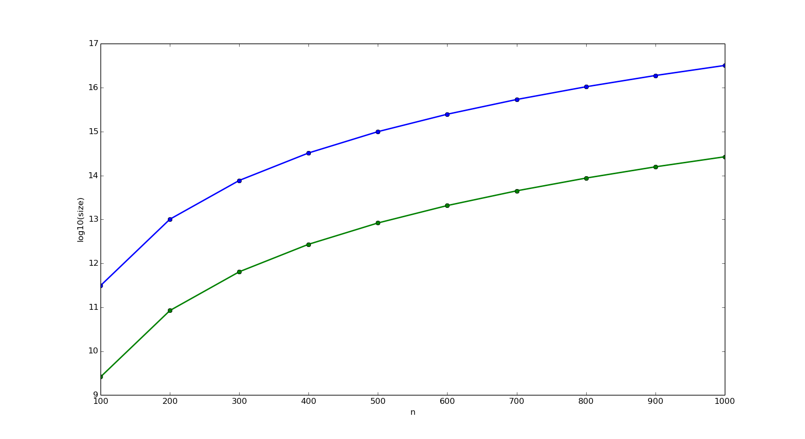
(a) First bound: smaller than $(2n-1)^{d}$

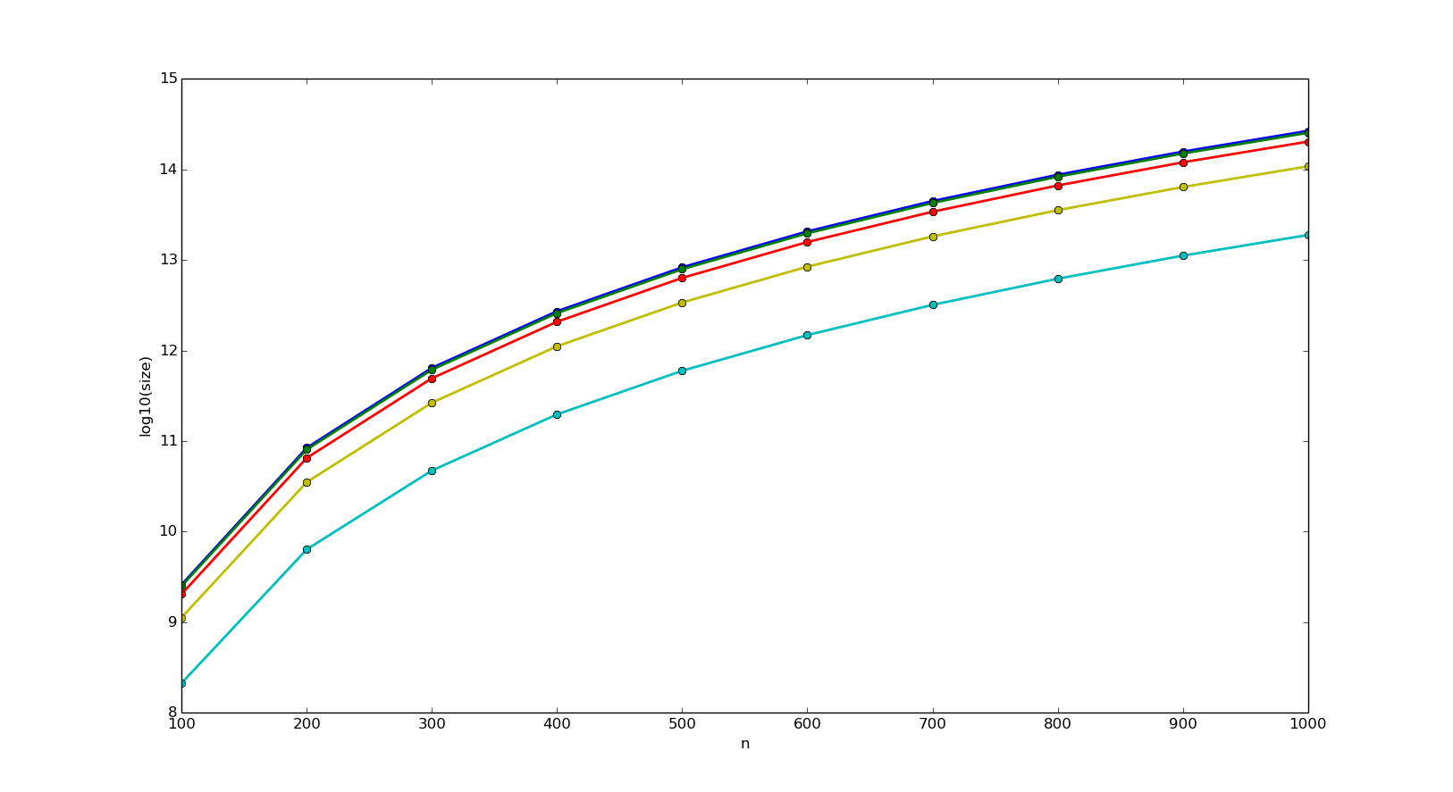
(b) Effect of $allprob$. (Top to bottom, $0,20,40,60,80$.)

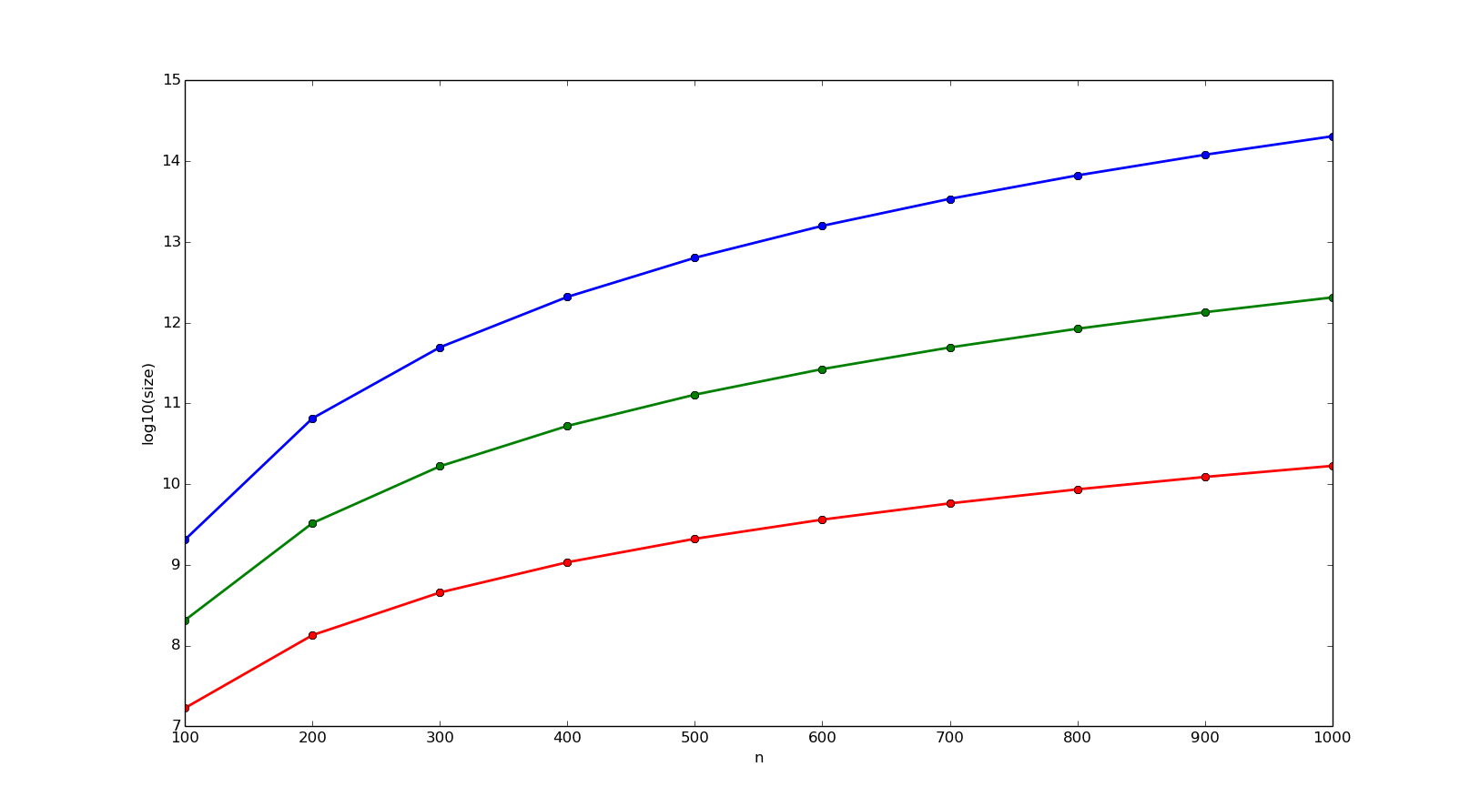
(c) Effect of narrow fields. $allprob=40$. (Lines, top to bottom, $5$ wide fields; $4$ wide + $1$ narrow; and $3$ wide + $2$ narrow. Narrow fields $2$ bits wide.)

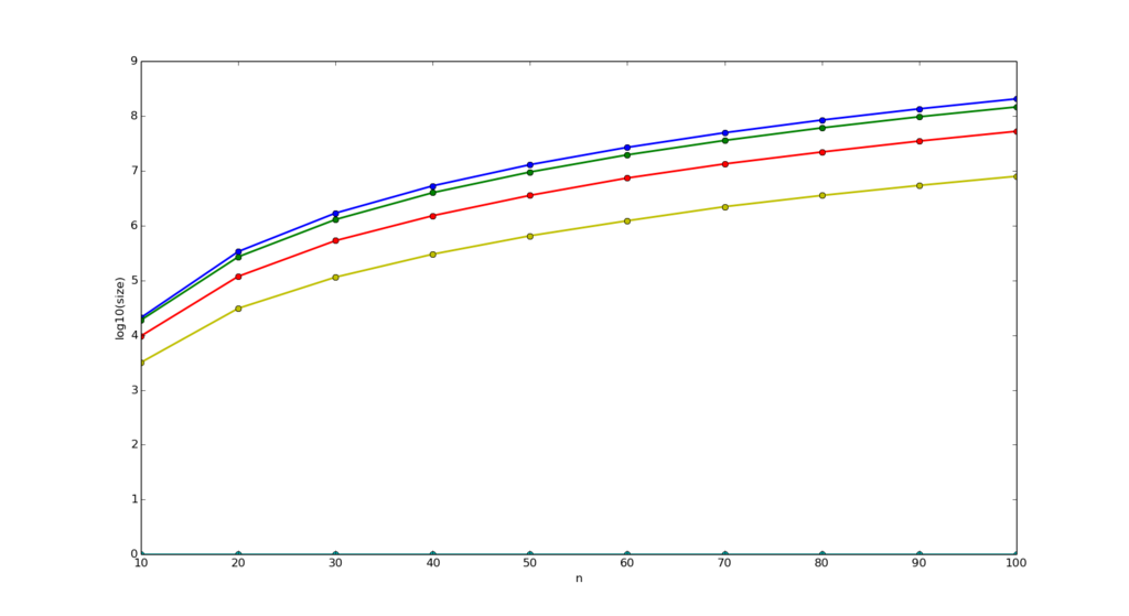
(d) Effect of $oneprob$. (Top to bottom, $0,20,40,60$.) $allprob=40$, $4$ wide + $1$ narrow field.

VII Related Work

Owing to the practical importance of policies, there exists a considerable body of work devoted to their study. A natural question is how this paper fits into the context of this research.

The first and most obvious area related to our work is the theory of policies. This area includes the design of algorithms and data structures for fast packet processing (i.e. resolution) as well as for verification of policies. Policies have been represented as tries [5] and lookup-tables by Waldvogel [6] and Gupta [7]. As preprocessing can be expensive, solutions have been developed by Suri[8] using B-trees, and by Sahni and Kim[9] using red-black trees and skip lists; these solutions allow fast update, and also perform (longest prefix) matching in $O(\log n)$ time.

Our work not only advances the theory of policies by providing an exact bound on the size of the policy decision diagram [2], but also proposes new metrics for the complexity of a policy, and shows why the algorithms for fast resolution and verification are tractable in practice. Our new metrics (fieldwidth, allprob and oneprob) make it possible to answer if a policy will have a decision diagram of tractable size.

More generally, the analysis of policies includes the study of anomalies [10], inter-rule conflicts [11], redundancies, and so on. For example, Frantzen [12] provides a framework for understanding the vulnerabilities in a firewall, and Blowtorch [13] is a framework to generate packets for testing. These algorithms depend on the complexity of a policy, as measured by the size of its decision diagram; our work sheds light on why they are practical to use.

Finally, our work impacts the study of high-performance architecture for fast packet resolution. High-throughput systems, such as backbone routers, make use of special hardware - ternary content addressable memory[14], ordinary RAM, pipelining systems [15], and so on. But these systems are very expensive, as well as limited in the size of policies they can accommodate. Therefore, there is active research on algorithms to optimize policies, such as Liu’s TCAM Razor[14]. This paper shows how, using our concept of rules in play, we can improve upon these algorithms to create truly minimum policies (rather than just locally minimal ones).

VIII Concluding Remarks

In this paper, we make two contributions to the theory of policies and their complexity. Our first contribution is to introduce the concept of “rules in play”, which enables us to calculate the actual upper bound on the size of the policy decision diagram. We also show why this size does not grow explosively for practical policies, and introduce new metrics for the complexity of a policy. These metrics (oneprob, allprob and fieldwidth) are not only simple to compute (one pass through the policy, $O(nd)$ time), but also have a dramatic effect on the behavior of policy algorithms. Thus, our work provides an explanation for the “unreasonable effectiveness” of practical decision diagram based algorithms: their running time is not really $O(n^{d})$, but depends on our new metrics also, and practical policies have tractable values for these new metrics.

Our second contribution is that, using rules in play, we propose the first optimization algorithm that can produce a truly minimum-length policy (rather than simply a minimal one, as can be found by removing redundant rules from the policy until no redundancy remains).

Our work on decision diagrams suggests several problems for further study. How do our metrics influence other measures of complexity, such as how many rules the average rule in a policy overlaps with? Can they be further refined (for example, by taking the oneprob and allprob field by field, rather than one measure for the whole policy)? And how do they influence other algorithms and data structures in policy research, such as decision-diagram compression by Bit Weaving [16]? For our own future work, we are focusing on the last of these questions. We also aim to improve our new algorithm for policy optimization, so as to make it fast enough for practical use.

References

- [1] E. Al-shaer, W. Marrero, A. El-atawy, and K. Elbadawi, “Network configuration in a box: Towards end-to-end verification of network reachability and security,” 2009.
- [2] A. X. Liu and M. G. Gouda, “Firewall policy queries,” IEEE Transactions on Parallel and Distributed Systems, vol. 20, no. 6, pp. 766–777, 2009.
- [3] H. B. Acharya, “On rule width and the unreasonable effectiveness of policy verification,” in IEEE 39th Conference on Local Computer Networks, LCN 2014, Edmonton, AB, Canada, 8-11 September, 2014, 2014, pp. 314–321.
- [4] A. Khoumsi, W. Krombi, and M. Erradi, “A formal approach to verify completeness and detect anomalies in firewall security policies,” in Foundations and Practice of Security, 2014, pp. 221–236.
- [5] K. Sklower, “A tree-based routing table for berkeley unix,” in Technical report, University of California, 1993.
- [6] M. Waldvogel, G. Varghese, J. Turner, and B. Plattner, “Scalable high speed ip routing lookups,” in Proceedings of ACM SIGCOMM, 1997, p. 25–36.
- [7] P. Gupta, S. Lin, and N. McKeown, “Routing lookups in hardware at memory access speeds,” in Proceedings of IEEE INFOCOM, 1998.
- [8] S. Suri, G. Varghese, and P. Warkhede, “Multiway range trees: Scalable ip lookup with fast updates,” in GLOBECOM, 2001.
- [9] S. Sahni and K. Kim, “O(log n) dynamic packet routing,” in IEEE Symposium on Computers and Communications, 2002.
- [10] H. H. Hamed, E. S. Al-Shaer, and W. Marrero, “Modeling and verification of ipsec and vpn security policies,” in ICNP, 2005, pp. 259–278.
- [11] D. Eppstein and S. Muthukrishnan, “Internet packet filter management and rectangle geometry,” in SODA, 2001, pp. 827–835.
- [12] M. Frantzen, F. Kerschbaum, E. E. Schultz, and S. Fahmy, “A framework for understanding vulnerabilities in firewalls using a dataflow model of firewall internals,” Computers & Security, vol. 20, no. 3, pp. 263–270, 2001.
- [13] D. Hoffman and K. Yoo, “Blowtorch: a framework for firewall test automation,” in Proceedings of the 20th IEEE/ACM international Conference on Automated software engineering, 2005, pp. 96–103.
- [14] D. Shah and P. Gupta, “Fast updating algorithms for tcams,” IEEE MICRO, vol. 21, no. 1, p. 36–47, 2001.
- [15] A. Basu and G. Narlika, “Fast incremental updates for pipelined forwarding engines,” in Proceedings of IEEE INFOCOM, 2003.
- [16] C. R. Meiners, A. X. Liu, and E. Torng, “Bit weaving: A non-prefix approach to compressing packet classifiers in tcams,” IEEE/ACM Trans. Netw., vol. 20, no. 2, pp. 488–500, 2012.