Adiabatic excitation of a confined particle in one dimension with a variable infinitely sharp wall

Abstract

It is shown that adiabatic cycles excite a quantum particle, which is confined in a one-dimensional region and is initially in an eigenstate. During the cycle, an infinitely sharp wall is applied and varied its strength and position. After the completion of the cycle, the state of the particle arrives another eigenstate. It is also shown that we may vary the final adiabatic state by choosing the parameters of the cycle. With a combination of these adiabatic cycles, we can connect an arbitrary pair of eigenstates. Hence, these cycles may be regarded as basis of the adiabatic excitations. A detailed argument is provided for the case that the particle is confined by an infinite square well. This is an example of exotic quantum holonomy in Hamiltonian systems.

I Introduction

An adiabatic process, also referred to as an adiabatic passage, offers a simple and robust way to control a quantum system Messiah (1999). An adiabatic passage connects a stationary state of the initial system with another stationary state of the final system through a slow variation of an external field, for example. This has been investigated both experimentally and theoretically to a variety of microscopic systems, e.g., atoms and molecules Rice and Zhao (2000); Shapiro and Brumer (2012); Shore (2011).

We here focus on the adiabatic passage along a closed cycle in the adiabatic parameter space. This corresponds to the case, for example, where the external field is applied only during a cycle, and is off before and after the cycle. One may expect that the adiabatic cycle induces no change, since there is no external field to keep the final state away from the initial one. This argument, however, has counterexamples. A famous one is the appearance of the geometric phase factor Berry (1984), which is also referred to as the quantum holonomy Simon (1983). Furthermore, an adiabatic cycle may deliver a stationary state into another stationary state. This can be regarded as an permutation of eigenspaces. Since this is analogous with the quantum holonomy, we call such an excitation due to adiabatic cycles an exotic quantum holonomy (EQH). Examples of EQH are reported through theoretical studies Cheon (1998); Tanaka and Cheon (2015).

In atomic and molecular systems, there are many studies of population transfers with the oscillating classical electromagnetic field both in theory and experiments. Among them, stimulated Raman adiabatic passage (STIRAP) Rice and Zhao (2000); Shapiro and Brumer (2012); Shore (2011) employs an adiabatic cycle made of quasienergies, which is the counterpart of eigenenergy in periodically driven systems Zel’dovich (1967). Its adiabatic cycle passes through a crossing point of quasienergies to realize the adiabatic excitation (or its inverse) Guérin et al. (2001); Yatsenko et al. (2002). Hence, STIRAP can be considered as an example of EQH. On the other hand, it has been shown that, even in the absence of level crossings, periodically driven systems may exhibit EQH Tanaka and Miyamoto (2007); Miyamoto and Tanaka (2007).

In this manuscript, we offer another example of EQH. This example consists of a particle confined in one-dimensional region, where a slowly varying wall is applied to make cycles. We assume that the time-dependent wall is described by a potential, which is propotional to the $\delta$-function. We call it a $\delta$-wall.

Since our model is described by a slowly time-dependent Hamiltonian, EQH is governed by the parametric dependence of eigenenergies, instead of quasienergies. This is in contrast with the examples with oscillating external field mentioned above. Also, our model is far simpler than the known examples of EQH in Hamiltonian systems, for example, a particle under the generalized pointlike potential Cheon (1998) and a quantum graph with a $4$-vertex Cheon et al. (2013). Experimental realizations of our model may be feasible within the current state of art, as is suggested by the realization of optical box trap made of two thin walls Meyrath et al. (2005),

We show that the adiabatic cycles of the present model may have qualitatively distinct result. Namely, by adjusting the parameters of the adiabatic cycle (i.e., the initial and final positions of the $\delta$-wall), we may vary the final stationary state. Also, by combining these cycles, we can connect an arbitrary adiabatic state. In this sense, these cycles form the basis of adiabatic excitations. In particular, we will examine two kinds of adiabatic cycles, which induces different permutations of eigenspaces. One is denoted as $C_{\rm X}$, which involves an insertion, a move, and a removal of the $\delta$-wall. Although this resembles a simple thermodynamic process Kim et al. (2011), its consequence would have no similarity in thermodynamics. Namely, we will show that the final state of the adiabatic cycle $C_{\rm X}$ is different from the initial one, depending on the positions of the wall. In other words, $C_{\rm X}$ may induce an excitation of the system. Another example $C_{\rm Y}$ involves an insertion, a flip, and a removal of the wall. The eigenspace permutation induced by $C_{\rm Y}$ resembles the one found in the Lieb-Liniger model Lieb and Liniger (1963), where all eigenspaces are excited at a time Yonezawa et al. (2013).

The plan of this manuscript is the following. We introduce our model in Section II and provide an exact analysis of the application of the $\delta$-wall in Section III. The adiabatic cycles $C_{\rm X}$ and $C_{\rm Y}$ are examined in Sections IV and V, respectively. Also in Sections IV, we show that a combination of $C_{\rm X}$’s adiabatically connects an arbitrary pair of eigenstates. Section VI is dedicated to conclusion.

II A confined 1-d particle with a $\delta$-wall

In this section, we introduce a confined 1-d particle with a $\delta$-wall. Suppose that a particle is confined within a one-dimensional region, whose position is denoted by $x$. The particle is described by a Hamiltonian $H_{0}=T+V_{0}(x)$, where $T\equiv p^{2}/2$ and $V_{0}(x)$ are the kinetic term and the confinement potential, respectively, and the particle mass is chosen to be unity.

Although the following argument is applicable to a wide class of confinement potentials $V_{0}(x)$ as long as $H_{0}$ has several bound states and has no spectral degeneracy, it is convenient to employ an infinite square well to explain the concept. We assume $V_{0}(x)=0$ for $0\leq x\leq L$, and $V_{0}(x)=\infty$ otherwise. As for the infinite square well, the eigenenergies of $H_{0}$ are $E^{(0)}_{n}=(\hbar\pi n/L)^{2}/2$ ($n=1,2,\dots$). Let $|{}n{}\rangle$ denote the corresponding normalized stationary state.

We introduce an additional $\delta$-wall, where the whole system is described by the Hamiltonian

$$H(g,X)\equiv H_{0}+g\delta(x-X).$$ (1)

We assume that we may vary the strength $g$ and position $X$ of the wall. Let $E_{n}(g,X)$ be an eigenenergy of $H(g,X)$ for $-\infty<g<\infty$, i.e.,

$$H(g,X)|{}n(g,X){}\rangle=E_{n}(g,X)|{}n(g,X){}\rangle,$$ (2)

where we impose $E_{n}(0,X)=E_{n}^{(0)}$ and $|{}n(0,X){}\rangle=|{}n{}\rangle$. We refer that an infinite square well with a $\delta$-wall was examined in Refs. Flügge (1971); Ushveridze (1988).

III Adiabatic application of $\delta$-wall

We examine the adiabatic insertion or removal of the $\delta$-wall, where the strength $g$ is varied while the position $X$ is fixed. The following analysis tells us how the eigenstates and eigenvalues of the unperturbed system (i.e, $g=0$) are connected to the ones in the limit $g\to\infty$.

First, we examine the “exceptional” case. Suppose that the node of the eigenfunction $\langle{}x{}|{}n_{0}(g_{0},X){}\rangle$ coincides with the position of the $\delta$-wall, i.e.,

$$\langle{}X{}|{}n_{0}(g_{0},X){}\rangle=0,$$ (3)

which implies $|{}n_{0}(g,X){}\rangle=|{}n_{0}{}\rangle$ and $E_{n_{0}}(g,X)=E_{n}^{(0)}$ for an arbitrary $g$, as is shown in the following. Since $H(g,X)$ satisfies

$$H(g,X)=H(g_{0},X)+(g-g_{0})\delta(x-X)$$ (4)

from Eq. (1), we obtain $H(g,X)|{}n_{0}(g_{0},X){}\rangle=E_{n_{0}}(g_{0},X)|{}n_{0}(g_{0},X){}\rangle+(g-g_{0})\delta(x-X)|{}n_{0}(g_{0},X){}\rangle$. For an arbitrary normalized state $|{}\phi{}\rangle$, we find

$$\langle{}\phi{}|H(g,X)|{}n_{0}(g_{0},X){}\rangle=E_{n_{0}}(g_{0},X)\langle{}\phi{}|{}n_{0}(g_{0},X){}\rangle,$$ (5)

because of Eq. (3). Hence we conclude $H(g,X)|{}n_{0}(g_{0},X){}\rangle=E_{n_{0}}(g_{0},X)|{}n_{0}(g_{0},X){}\rangle$, which implies $|{}n_{0}(g,X){}\rangle=|{}n_{0}{}\rangle$ and $E_{n_{0}}(g,X)=E_{n}^{(0)}$. We note that the condition Eq. (3) is equivalent to $\langle{}X{}|{}n_{0}{}\rangle=0$.

Since the analysis of exceptional levels are completed, we exclude them in the following. Namely, we focus on the levels whose unperturbed eigenstates satisfy $\langle{}X{}|{}n{}\rangle\neq 0$, which ensures that $\langle{}X{}|{}n(g,X){}\rangle\neq 0$ holds for an arbitrary $g$.

We show that there is no level crossing among these levels. Let us examine a pair of the levels $n$ and $n^{\prime}$, where $E_{n}^{(0)}<E_{n^{\prime}}^{(0)}$ is assumed. We find from Eqs. (2) and (4),

$$\left\{E_{n}(g,X)-E_{n^{\prime}}(g^{\prime},X)\right\}\langle{}n(g,X){}|{}n^{\prime}(g^{\prime},X){}\rangle$$

$${}\qquad\qquad=(g-g^{\prime})\langle{}n(g,X){}|{}X{}\rangle\langle{}X{}|{}n^{\prime}(g^{\prime},X){}\rangle.$$ (6)

When $g\neq g^{\prime}$ holds, we obtain

$$\left\{E_{n}(g,X)-E_{n^{\prime}}(g^{\prime},X)\right\}\langle{}n(g,X){}|{}n^{\prime}(g^{\prime},X){}\rangle\neq 0,$$ (7)

because of $\langle{}n(g,X){}|{}X{}\rangle\langle{}X{}|{}n^{\prime}(g^{\prime},X){}\rangle\neq 0$. Namely, we find

$$E_{n}(g,X)\neq E_{n^{\prime}}(g^{\prime},X)\quad\text{for $g\neq g^{\prime}$}.$$ (8)

Since $E_{n}(g,X)$ monotonically increases with $g$ strictly, we conclude

$$E_{n}(g,X)<E_{n}(\infty,X)\leq E_{n^{\prime}}(-\infty,X)<E_{n^{\prime}}(g,X)$$ (9)

for an arbitrary $-\infty<g<\infty$. Thus there is no level crossing between $n$-th and $n^{\prime}$-th levels.

A simple condition that ensures the absence of level crossing among the levels $n<n^{*}$, where $n^{*}$ defines a cutoff, is $\langle{}X{}|{}n{}\rangle\neq 0$ holds for all $n<n^{*}$. For the infinite square well, all unperturbed eigenstates satisfy this condition as long as $X/L$ is an irrational number.

IV Cycle with expansion/compression

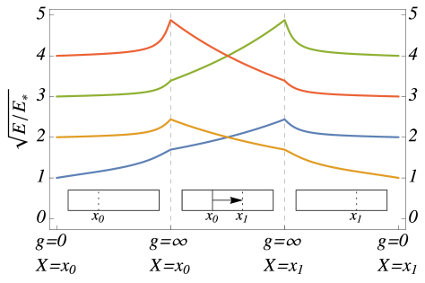
Figure 1: (Color online) Parametric evolution of the eigenenergies of a particle confined in an infinite square well, along the closed cycle $C_{\rm X}(x_{0},x_{1})$. The lowest four eigenenergies are shown. We choose $x_{0}=0.41L$ and $x_{1}=0.59L$, where $L$ is the size of the well. $E_{*}\equiv\frac{1}{2}(\hbar\pi/L)^{2}$ is the ground energy of the unperturbed system. The insets illustrate the position of the $\delta$-wall in each process schematically. (Left) A $\delta$-wall is initially placed at $X=x_{0}$ (dotted line) with its strength $g=0$. While increasing $g$ to $\infty$, there is no level crossing. (Middle) The impermeable $\delta$-wall (i.e., $g=\infty$) is moved from $x_{0}$ (full line) to $x_{1}$ (dashed line). A level crossing occurs at $X=L/2$. (Right) While $X=x_{1}$ is kept fixed, $g$ is decreased to $0$ to finish the cycle. There is no level crossing in this process. As a result, the cycle interchanges the ground and first-excited energies. The second and third-excited eigenenergies are also interchanged. The adiabatic time evolution follows along these lines. We note that the horizontal axis of the left and right part is linear in $\tan^{-1}g$.

We examine an adiabatic cycle $C_{\rm X}(x_{0},x_{1})$, which consists of an insertion, a move, and a removal of the $\delta$-wall. In particular, we impose that, during the second process, the $\delta$-wall is impermeable, i.e., $g=\infty$, to completely divide the confinement well into two regions.

The key to realize the adiabatic excitation through $C_{\rm X}$ is to utilize the level crossing during the second process. The same concept has been utilized in Refs. Guérin et al. (2001); Yatsenko et al. (2002); Cheon et al. (2009) to realize the adiabatic excitations along cycles. Although the level crossings are generally fragile against perturbations according to Wigner and von Neumann’s theorem Landau and Lifshitz (1965a), this theorem is inapplicable to our case since the system is completely divided into two parts. In reality, if we take into account the imperfection of the impermeable wall, e.g. the effect of tunneling, the spectral degeneracy may be lifted. There we need to resort to the diabatic evolution to go across the avoided crossing in order to approximately realize the adiabatic excitation Cheon et al. (2009).

We assume that the system is initially in a stationary state $|{}n{}\rangle$, i.e., the $n$-th excited state of the initial system $\hat{H}_{0}$. We will show that the final state is the $(n+1)$-th excited state, if we appropriately choose $x_{0}$ and $x_{1}$, i.e., $C_{\rm X}(x_{0},x_{1})$ delivers the initial stationary state to its higher neighboring state. For simplicity, we assume in this section that the confinement potential is the infinite square well, and $x_{j}/L$ ($j=0,1$) is irrational.

A precise definition of $C_{\rm X}(x_{0},x_{1})$ is shown. First, the wall is adiabatically inserted at $x_{0}$. Namely, the strength $g$ is adiabatically increased from $0$ to $\infty$, while the position is kept fixed at $X=x_{0}$. After the completion of this process, the $\delta$-wall is impermeable, i.e., the confinement is divided into two regions. Second, the impermeable wall is moved adiabatically from $x_{0}$ to $x_{1}$. If $x_{0}<x_{1}$ ($x_{0}>x_{1}$) holds, we say that the left (right) well is expanded while the other well is compressed. Third, the wall is adiabatically removed, where the strength $g$ is adiabatically decreased from $\infty$ to $0$ while the position is kept fixed at $X=x_{1}$. After the completion of this process, the system is described by the unperturbed Hamiltonian $H_{0}$ again.

During the first process, the state vector of the system is $|{}n(g,x_{0}){}\rangle$, up to a phase factor. There is no level crossing $0\leq g<\infty$, since we choose $x_{0}/L$ is irrational (see Sec. III). Hence the system is always in $n$-th excited state. This implies that the system is also in the $n$-th state right before the second process. Similarly, the system is in the $(n+1)$-th excited state right after the second process.

We explain how the $n$-th and $(n+1)$-th states are connected by the second process, i.e., the moving the impermeable wall from $x_{0}$ to $x_{1}$, through a level crossing. We examine this process by introducing another quantum numbers $m_{\rm L}$ and $m_{\rm R}$ of the separated systems.

Since we assume that $V_{0}(x)$ is the infinite square well, the system is divided into two infinite square wells during the second process. The left and right wells are placed at $0\leq x\leq X$ and $X\leq x\leq L$, respectively. We introduce two quantum numbers $m_{\rm L}{}$ and $m_{\rm R}{}$, which describes the particle confined in the left and right wells, respectively, under the presence of the impermeable wall. The eigenenergies are $E_{{\rm L},m_{\rm L}{}}(X)=(\hbar\pi m_{\rm L}{}/X)^{2}/2$ and $E_{{\rm R},m_{\rm R}{}}(X)=(\hbar\pi m_{\rm R}{}/(L-X))^{2}/2$.

We examine the level crossing consists of $m_{\rm L}{}$-th and $m_{\rm R}{}$-th states. By solving $E_{{\rm L},m_{\rm L}{}}(X)=E_{{\rm R},m_{\rm R}{}}(X)$, we find the degeneracy point

$$X_{m_{\rm L}{},m_{\rm R}{}}\equiv\frac{m_{\rm L}{}}{m_{\rm L}{}+m_{\rm R}{}}L.$$ (10)

Since $E_{{\rm L},m_{\rm L}{}}(X)$ and $E_{{\rm R},m_{\rm R}{}}(X)$ monotonically depend on $X$, $E_{{\rm R},m_{\rm R}{}}(X)\gtrless E_{{\rm L},m_{\rm L}{}}(X)$ holds if $X\gtrless X_{m_{\rm L}{},m_{\rm R}{}}$.

In the following, we assume that there is no other level crossing that involves the eigenstates $m_{\rm L}{}$ and $m_{\rm R}{}$ in the second process $x_{0}\leq X\leq x_{1}$. This condition is

$$\max(X_{m_{\rm L}{}-1,m_{\rm R}{}},X_{m_{\rm L}{},m_{\rm R}{}+1})<x_{0}<X_{m_{\rm L}{},m_{\rm R}{}}$$

$$<x_{1}<\min(X_{m_{\rm L}{}+1,m_{\rm R}{}},X_{m_{\rm L}{},m_{\rm R}{}-1}),$$ (11)

and $x_{0}<X_{m_{\rm L}{},m_{\rm R}{}}<x_{1}$.

Now we determine the quantum number $n$ for $m_{\rm L}{}$-th and $m_{\rm R}{}$-th states at the initial point of the first process, where $X=x_{0}$ holds. Let $n_{\rm L}$ and $n_{\rm R}$ denote the values of $n$ for $m_{\rm L}{}$-th and $m_{\rm R}{}$-th states, respectively. From the condition for $x_{0}$ examined above, we find $n_{\rm L}=n_{\rm R}+1$. In the left (right) well, there are $m_{\rm L}{}-1$ ($m_{\rm R}{}-1$) stationary states below the $m_{\rm L}{}$($m_{\rm R}{}$)-th stationary state. Hence, we obtain $n_{\rm R}=(m_{\rm L}{}-1)+(m_{\rm R}{}-1)+1=m_{\rm L}{}+m_{\rm R}{}-1$, and $n_{\rm L}=m_{\rm L}{}+m_{\rm R}{}$.

On the other hand, at the final point of the process (3), i.e., at $X=x_{1}$, the order of the $m_{\rm L}{}$-th and $m_{\rm R}{}$-th states is reversed, i.e., $n_{\rm L}+1=n_{\rm R}$, which implies $n_{\rm L}=m_{\rm L}{}+m_{\rm R}{}-1$ and $n_{\rm R}=m_{\rm L}{}+m_{\rm R}{}$.

The conditions for $x_{0}$ and $x_{1}$ can be simplified if we specify the crossing point $X_{m_{\rm L}{},m_{\rm R}{}}$ by its initial lower quantum number $n$ as $m_{\rm R}{}=\lfloor{(n+1)/2}\rfloor$ and $m_{\rm L}=n+1-m_{\rm R}$, for example, where $\lfloor{x}\rfloor$ is the maximum integer less than $x$. When $n$ is odd, we find

$$\frac{n+1}{2(n+2)}L<x_{0}<\frac{1}{2}L<x_{1}<\frac{n+3}{2(n+2)}L.$$ (12)

On the other hand, when $n$ is even, we find

$$\frac{1}{2}L<x_{0}<\frac{n+2}{2(n+1)}L<x_{1}<\frac{n+4}{2(n+2)}L.$$ (13)

We summarize the argument above to describe the adiabatic evolution along the cycle $C_{\rm X}(x_{0},x_{1})$. The system is prepared to be $|{}n{}\rangle$ initially. We utilize the crossing point $X_{m_{\rm L}{},m_{\rm R}{}}$ at the second process, where $1\leq m_{\rm R}{}\leq n$ and $m_{\rm L}{}=n+1-m_{\rm R}{}$ is assumed. During the first process, the system is in $|{}n(g,x_{0}){}\rangle$ up to the phase factor. Hence the system is in $n$-th excited state. At the end of the first process, the state $|{}n(g,x_{0}){}\rangle$ is $m_{\rm R}{}$-th state in the right well. Also, during the second process, the state keeps to stay in $m_{\rm R}{}$-th state in the right well. At the same time, the systems is in $(n+1)$-th state of the whole system. During the third process, the system is in $|{}n+1(g,x_{1}){}\rangle$ up to the phase factor. Hence, the final state of the cycle is $|{}n+1{}\rangle$. In this sense, the adiabatic excitation from $|{}n{}\rangle$ to $|{}n+1{}\rangle$ is completed. We depict the examples that adiabatically connects the ground and first excited states in Figs. 1 and 2.

Figure 2: (Color online) Parametric evolution of an eigenfunction along $C_{\rm X}(x_{0},x_{1})$. During the insertion process, the initial eigenfunction $\langle{}x{}|{}1{}\rangle$ (nodeless, full line) at $g=0$ becomes $\langle{}x{}|{}1(10g_{*},x_{0}){}\rangle$ (dashed), where $g_{*}=\pi\hbar^{2}/(2L)$, and is finally confined at the right box (not shown here). During the removal process, the initial eigenfunction localized in the right box ($x_{1}<x<L$, not shown here) becomes $\langle{}x{}|{}2(10g_{*},x_{1}){}\rangle$ (dotted). The final eigenfunction is $\langle{}x{}|{}2{}\rangle$ (with a node, full line). The positions of the $\delta$-wall at the insertion and removal are indicated by dashed vertical lines. We choose $L=1$. Other parameters are the same as in Fig. 1.

We note that, from the construction, the repetition of the cycle $C_{\rm X}(x_{0},x_{1})$ two times, $|{}n{}\rangle$ is delivered to the initial state $|{}n{}\rangle$, so is $|{}n+1{}\rangle$. Hence the inverse of $C_{\rm X}(x_{0},x_{1})$ delivers $|{}n+1{}\rangle$ to $|{}n{}\rangle$.

We also note that an arbitrary pair of the eigenstates of $H_{0}$ can be adiabatically connected, if we appropriately combine adiabatic cycles $C_{\rm X}(x_{0},x_{1})$ with various values of $x_{0}$ and $x_{1}$. For example, the cycle shown in Fig. 1 connects two pairs $(n=1,n=2)$ and $(n=3,n=4)$, whereas the cycle in Fig. 3 connects the pair $(n=2,n=3)$. Hence, the ground state $|{}1{}\rangle$ can be connected to the stationary state $|{}4{}\rangle$ by a combination of these two cycles. In this sense, these cycles can be regarded as basis of the adiabatic excitations.

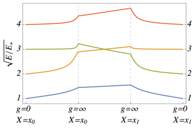
Figure 3: (Color online) Parametric evolution of eigenenergies along $C_{\rm X}(x_{0},x_{1})$ with $x_{0}=0.31L$ and $x_{1}=0.36L$. While the eigenenergies of the first and second excited states are interchanged, there is no effect on the ground and third excited states.

V Cycle with $\delta$-wall flip

Figure 4: (Color online) Parametric evolution of eigenenergies along $C_{\rm Y}(x_{0})$ with $x_{0}=0.41L$. The horizontal axis is linear in $\tan^{-1}g$, and we set $g_{*}=\pi\hbar^{2}/(2L)$. The left half and the right half corresponds the first and the third process of $C_{\rm Y}(x_{0})$ respectively. After the completion of $C_{\rm Y}(x_{0})$, all eigenenergies are delivered to higher neighboring eigenenergies.

We proceed to examine the cycle $C_{\rm Y}(x_{0})$ that involves an insertion, a flip, and a removal of the $\delta$-wall placed at $x_{0}$. We will show that $C_{\rm Y}(x_{0})$ delivers an arbitrary stationary state $|{}n{}\rangle$ to higher neighboring state $|{}n+1{}\rangle$, if $x_{0}$ is chosen appropriately. Hence the resultant permutation of eigenspaces is different from the one induced by $C_{X}(x_{0},x_{1})$.

Our definition of $C_{\rm Y}(x_{0})$ is the following. First, the strength of the $\delta$-wall $g$ is adiabatically increased from $0$ to $\infty$, i.e., the first process is the same with $C_{X}(x_{0},x_{1})$. Second, $g$ is suddenly changed from $\infty$ to $-\infty$ to flip the wall. Third, $g$ is adiabatically increased from $-\infty$ to $0$ to remove the wall.

We note that $C_{\rm Y}(x_{0})$ resembles a cycle that passes Tonks-Girardeau and super-Tonks-Girardeau regimes of the Lieb-Liniger model Haller et al. (2009). In this cycle, the strength of the two-body contact interaction of Bose particles is varied from zero to $\infty$, then is changed from $\infty$ to $-\infty$ suddenly, and is finally increased from $-\infty$ to zero. The adiabatic cycle excites the system consists of the Bose particles Yonezawa et al. (2013).

We examine the parametric evolution of $E_{n}(g,X)$ along $C_{\rm Y}(x_{0})$ (see, Fig. 4). As is done in the previous section, we assume that the confinement potential is the infinite square well and $x_{0}/L$ is irrational.

The parametric evolution along the first process is examined in the previous section: $E_{n}(g,X)$ monotonically increases with $g$, and has no crossing with other levels.

To examine the second process, i.e. the $\delta$-wall flip, we utilize the fact that an eigenenergy $E$ satisfies a transcendental equation, which is determined by the connection problem of the eigenfunction at $x_{0}$ Landau and Lifshitz (1965b). We may examine the transcendental equation with a small parameter $g^{-1}$ Ushveridze (1988), which concludes that the $n$-th eigenenergy is connected to the $n^{*}$-th eigenenergy at $g=-\infty$, i.e,

$$E_{n}(\infty,x_{0})=E_{n^{*}}(-\infty,x_{0}),$$ (14)

where $n^{*}$ is an integer.

The following proof of $n^{*}=n+1$ is divided into two parts. First, we show $n<n^{*}$. Since $E_{n}(g,x_{0})$ monotonically increases with $g$ (see, Sec. III), we obtain $E^{(0)}_{n}<E_{n}(\infty,x_{0})$ and $E_{n^{*}}(-\infty,x_{0})<E^{(0)}_{n^{*}}$. We find, from Eq. (14), $E^{(0)}_{n}<E^{(0)}_{n^{*}}$, which implies $n<n^{*}$. Second, we show $n^{*}\leq n+1$ by contradiction. Assuming $n^{*}>n+1$, we find $E^{(0)}_{n+1}<E_{n+1}(\infty,x_{0})\leq E_{n^{*}}(-\infty,x_{0})$ holds from Eq. (9). Using Eq. (14), we obtain $E^{(0)}_{n+1}<E_{n}(\infty,x_{0})$, which contradicts with Eq. (9). Namely $n^{*}\leq n+1$ holds. Thus we conclude $n^{*}=n+1$.

The analysis of the third process can be carried out as in the case for the first process. Hence, we conclude that the eigenenergy monotonically increases from $E_{n+1}(-\infty,x_{0})$ to $E_{n+1}^{(0)}$ during the third process.

In summary, the adiabatic time evolution along $C_{\rm Y}(x_{0})$ is the following. During the first process, the state is $|{}n(g,x_{0}){}\rangle$ up to a phase factor. The flip of the $\delta$-wall do not change the state. During the third process, the state is $|{}n+1(g,x_{0}){}\rangle$ up to a phase factor, and finally arrives at the $(n+1)$-th stationary state of the unperturbed system.

We remark on the inverse of $C_{\rm Y}(x_{0})$. In general, $C_{\rm Y}^{-1}(x_{0})$ adiabatically delivers an arbitrary stationary state, except the ground state, to the neighboring lower stationary state. On the other hand, if the system is initially in the ground state, the corresponding eigenenergy diverges to $-\infty$ as a result of the inverse cycle $C_{\rm Y}^{-1}(x_{0})$. The corresponding final state is strongly attracted to the $\delta$-wall with $g=-\infty$.

VI Summary and discussion

We have shown that a confined one-dimensional particle are excited by the adiabatic cycles $C_{\rm X}(x_{0},x_{1})$ and $C_{\rm Y}(x_{0})$, where the strength and the position of a $\delta$-wall is varied. Hence we have obtained another simple example of exotic quantum holonomy Tanaka and Cheon (2015).

We have shown a detailed analysis of the case that $V_{0}(x)$ is the infinite square well. In particular, an appropriate combination of $C_{\rm X}(x_{0},x_{1})$ adiabatically connects an arbitrary pairs of the stationary states of the unperturbed Hamiltonian $H_{0}$. In this sense, the adiabatic cycles $C_{\rm X}(x_{0},x_{1})$ and $C_{\rm Y}(x_{0})$ can be regarded as basis of the permutations of eigenstates. As an extension of the present work, it may be interesting to find a combination of the cycles to realize an arbitrary permutation of eigenspaces Leghtas et al. (2011).

At the same time, we have shown the basis to extend the present result to the cases with an arbitrary confinement potential $V_{0}(x)$. In particular, an exact analysis of the adiabatic application of the $\delta$-wall is shown, where the condition for the absence of the level crossing during the insert/removal of the $\delta$-wall under an arbitrary confinement potential $V_{0}(x)$ is clarified. Hence, it is straightforward to show that the adiabatic excitation is possible for an arbitrary confinement potential, as long as the unperturbed Hamiltonian has multiple bound states. The changes required to the present argument depends on the position of the nodes of the eigenfunctions of $H_{0}$.

The present scheme should be experimentally realized within the current state of art, e.g., an optical box trap made of a one-dimensional confinement and two Gaussian walls Meyrath et al. (2005). If an additional Gaussian wall approximates a $\delta$-wall well, the adiabatic excitation by cycles can be realized.

Finally, we briefly explain a possible application of the present work to produce dark solitons with multiple nodes in a cold atom Bose-Einstein condensate (BEC). This is based on the correspondence exploited in Refs. Karkuszewski et al. (2001); Damski et al. (2001), between higher excited states of a single particle system and dark solitons of the BEC. More precisely, it is shown that a diabatic process, i.e. an adiabatic process with a diabatic jump through very narrow level crossing, delivers the ground state of a single particle system to its first excited state, and that we may produce a dark soliton with a single node using a straightforward extension of the diabatic process to the BEC. Because of the resemblance with diabatic process studied in Refs. Karkuszewski et al. (2001); Damski et al. (2001), the adiabatic cycles in the present paper may produce dark solitons from its many-body ground states, when applied to the dilute Bose system. Moreover, an appropriate combination of the adiabatic cycles will produce the dark solitons with multiple nodes, which correspond to a higher excited state in the single particle system.

References

- Messiah (1999) A. Messiah, “Quantum mechanics,” (Dover, New York, 1999) Chap. 17.
- Rice and Zhao (2000) S. A. Rice and M. Zhao, Optical Control of Molecular Dynamics (Wiley-Interscience, New York, 2000).
- Shapiro and Brumer (2012) M. Shapiro and P. Brumer, Quantum Control of Molecular Processes, 2nd ed. (Wiley-VCH, Singapore, 2012).
- Shore (2011) B. W. Shore, Manipulating Quantum Structures Using Laser Pulses (Cambridge, Cambridge, 2011).
- Berry (1984) M. V. Berry, Proc. R. Soc. London A 392, 45 (1984).
- Simon (1983) B. Simon, Phys. Rev. Lett. 51, 2167 (1983).
- Cheon (1998) T. Cheon, Phys. Lett. A 248, 285 (1998).
- Tanaka and Cheon (2015) A. Tanaka and T. Cheon, Phys. Lett. A 379, 1693 (2015).
- Zel’dovich (1967) Y. B. Zel’dovich, Sov. Phys.–JETP 24, 1006 (1967).
- Guérin et al. (2001) S. Guérin, L. P. Yatsenko, and H. R. Jauslin, Phys. Rev. A 63, 031403(R) (2001).
- Yatsenko et al. (2002) L. P. Yatsenko, S. Guérin, and H. R. Jauslin, Phys. Rev. A 65, 043407 (2002).
- Tanaka and Miyamoto (2007) A. Tanaka and M. Miyamoto, Phys. Rev. Lett. 98, 160407 (2007).
- Miyamoto and Tanaka (2007) M. Miyamoto and A. Tanaka, Phys. Rev. A 76, 042115 (2007).
- Cheon et al. (2013) T. Cheon, A. Tanaka, and O. Turek, Acta Polytechnica 53, 410 (2013).
- Meyrath et al. (2005) T. P. Meyrath, F. Schreck, J. L. Hanssen, C.-S. Chuu, and M. G. Raizen, Phys. Rev. A 71, 041604(R) (2005).
- Kim et al. (2011) S. W. Kim, T. Sagawa, S. De Liberato, and M. Ueda, Phys. Rev. Lett. 106, 070401 (2011).
- Lieb and Liniger (1963) E. H. Lieb and W. Liniger, Phys. Rev. 130, 1605 (1963).
- Yonezawa et al. (2013) N. Yonezawa, A. Tanaka, and T. Cheon, Phys. Rev. A 87, 062113 (2013).
- Flügge (1971) S. Flügge, Practical Quantum Mechanics, Vol. 1 (Springer-Verlag, Berlin, 1971).
- Ushveridze (1988) A. G. Ushveridze, J. Phys. A. 21, 955 (1988).
- Cheon et al. (2009) T. Cheon, A. Tanaka, and S. W. Kim, Phys. Lett. A 374, 144 (2009).
- Landau and Lifshitz (1965a) L. D. Landau and E. M. Lifshitz, “Quantum mechanics,” (Pergamon Press, Oxford, 1965) Chap. XI, 2nd ed.
- Haller et al. (2009) E. Haller, M. Gustavsson, M. J. Mark, J. G. Danzl, , R. Hart, G. Pupillo, and H.-C. Nägerl, Science 325, 1224 (2009).
- Landau and Lifshitz (1965b) L. Landau and E. M. Lifshitz, “Quantum mechanics,” (Pergamon Press, Oxford, 1965) Chap. 3.
- Leghtas et al. (2011) Z. Leghtas, A. Sarlette, and P. Rouchon, J. Phys. B 44, 154017 (2011).
- Karkuszewski et al. (2001) Z. P. Karkuszewski, K. Sacha, and J. Zakrzewski, Phys. Rev. A 63, 061601(R) (2001).
- Damski et al. (2001) B. Damski, Z. P. Karkuszewski, K. Sacha, and J. Zakrzewski, Phys. Rev. A 65, 013604 (2001).