The deconfining phase transition of SO(N) gauge theories in 2+1 dimensions

Abstract

We calculate the deconfining temperature of $SO(N)$ gauge theories in 2+1 dimensions, and determine the order of the phase transition as a function of $N$, for various values of $N\in[4,16]$. We do so by extrapolating our lattice results to the infinite volume limit, and then to the continuum limit, for each value of $N$. We then extrapolate to the $N=\infty$ limit and observe that the $SO(N)$ and $SU(N)$ deconfining temperatures agree in that limit. We find that the the deconfining temperatures of all the $SO(N)$ gauge theories appear to follow a single smooth function of $N$, despite the lack of a non-trivial centre for odd $N$. We also compare the deconfining temperatures of $SO(6)$ with $SU(4)$, and of $SO(4)$ with $SU(2)\times SU(2)$, motivated by the fact that these pairs of gauge theories share the same Lie algebras.

1 Introduction

While a great deal is known about the non-perturbative physics of $SU(N)$ gauge theories from calculations on the lattice, much less is known about $SO(N)$ gauge theories. In this paper we will show that $SO(N)$ gauge theories in $2+1$ dimensions possess a deconfining phase transition at a finite temperature $T=T_{c}$, just like the deconfining transition in $SU(N)$ gauge theories. We will calculate its value and determine its nature for $N=4,5,6,7,8,9,12,16$. This will enable us to extrapolate to $N=\infty$ where we can compare to the $SU(\infty)$ extrapolated value Jack-Liddle:2008xr . This is interesting to do since $SO(N)$ and $SU(N)$ gauge theories have a common planar limit Lovelace:1982fk , and $SO(2N)$ and $SU(N)$ gauge theories are orbifold equivalent orbifold , so we expect that dimensionless ratios of common physical quantities, including the deconfining temperature, should be equal at $N=\infty$ Unsal:2006kx . We will perform further comparisons motivated by the fact that certain $SO(N)$ and $SU(N^{\prime})$ gauge theories share the same Lie algebras, i.e. $SO(3)$ and $SU(2)$, $SO(4)$ and $SU(2)\times SU(2)$, $SO(6)$ and $SU(4)$. To the extent that the difference in the global properties of the groups (such as the centre) is not important, we would expect the deconfining transition and temperature to be identical within each of these pairs of gauge theories, and this is something we shall attempt to check. Moreover assuming this identity, the known value of $T_{c}$ in $SU(2)$ provides us with a value for $SO(3)$, which we do not calculate directly (for reasons given below). In addition all these calculations will allow us to compare $SO(2N)$ and $SO(2N+1)$ theories, which is interesting because $SO(2N+1)$ gauge theories have a trivial center in contrast to the non-trivial $\mathbb{Z}_{2}$ center of $SO(2N)$ theories.

While the calculations in this paper are primarily intended to establish the presence of the finite $T$ transition and to investigate its properties, we shall choose to call it a deconfining transition, for both odd and even $N$, just like the one in $SU(N)$ gauge theories. Of course that assumes that these theories are linearly confining at low $T$. While we shall provide some evidence for confinement at low $T$ in this paper (see in particular the discussion in Section 3.3), the explicit evidence for the confinement being linear is given in our companion paper on the glueball spectra and string tensions Lau:aa , where we show that the energy of closed flux tubes is (roughly) proportional to their length for both odd and even $N$. Of course such numerical evidence possesses intrinsic limitations: we cannot distinguish between confinement that is exact and confinement to a very good approximation. However the quality of our numerical evidence is comparable to that which establishes linear confinement in $D=2+1$ $SU(N)$ gauge theories.

The paper is structured as follows. In Section 2, we briefly review some well-known relations between $SO(N)$ and $SU(N)$ gauge theories, both at small and at large $N$. In Section 3 we briefly describe the lattice setup, how to differentiate confining from non-confining phases, and we comment on what we know about confinement in $SO(N)$ gauge theories. In Section 4, we describe how we identify the location of the finite temperature transition and how we determine whether the transition is first or second order. Then in Section 5, we describe how to calculate on a lattice the physical quantities that we shall use in order to express the transition temperature in physical units. The next few sections contain our results. First, in Section 6 , we calculate the infinite volume limit for each of the $SO(N)$ gauge theories we consider, and hence the value of $T_{c}$ at various lattice spacings. Then, in Section 7, we use these values to calculate the continuum limit of the deconfining temperature for each group, briefly discussing the issues caused by the strong to weak coupling ‘bulk’ transition in $D=2+1$. We then proceed in Section 8 to calculate the large-$N$ limit of $T_{c}$ for $SO(2N)$ and $SO(2N+1)$ separately and together and in Section 9, we compare the $SO(N)$ and $SU(N)$ deconfining temperatures both at $N=\infty$, and for pairs of $SO(N)$ and $SU(N^{\prime})$ groups that share the same Lie algebra. Section 10, contains a summary of our conclusions. Appendix A contains our detailed tabulated results.

There are companion papers, both published Athenodorou:2015aa and in progress Lau:aa , that contain our results for the mass spectrum and string tension of $SO(N)$ gauge theories. The latter paper describes the Monte Carlo algorithm in more detail, as well as providing more discussion of the ‘bulk’ transition. An earlier paper Bursa:2013lq contained our first, exploratory estimates of $T_{c}$. The values in the present paper are much more accurate and supersede those earlier values, although they are in fact consistent within errors.

2 Relations between $SO(N)$ and $SU(N)$

2.1 Lie algebra equivalences

The implications of the Lie algebra equivalence between certain $SO(N)$ and $SU(N^{\prime})$ groups are discussed in more detail in Athenodorou:2015aa ; Lau:aa . Here we merely summarise some points that are relevant to our present calculations. If we assume that the global structure of the groups is irrelevant to the physics (an assumption which needs to be tested) then we expect that colour singlet quantities are the same within each pair of theories. For example the mass gap or the deconfining temperature. String tensions on the other hand are associated with a flux that is in a certain representation, and this needs to be matched between the theories. In the following we summarise some points that are relevant to the calculations in this paper.

The first equivalence is between the Lie algebras of $SO(3)$ and $SU(2)$. The $SO(3)$ fundamental representation is equivalent to the $SU(2)$ adjoint representation, so that the associated string tension should satisfy

$$\left.\sigma_{f}\right|_{so3}=\left.\sigma_{adj}\right|_{su2}.$$ (1)

Adjoint flux tubes in $SU(2)$ are not expected to be stable and can, for example, decay into glueballs. So one expects the same to be true for $SO(3)$ fundamental flux tubes. Of course, if the decay width is small enough, then just as for the mass of a narrow resonance, we can estimate a string tension. More importantly, glueball masses and $T_{c}$ should be the same within $SU(2)$ and $SO(3)$, and the coupling $g^{2}$ should satisfy Bursa:2013lq ; Lau:aa

$$\left.g^{2}\right|_{so3}=\left.4g^{2}\right|_{su2}.$$ (2)

In this paper we do not calculate $T_{c}$ for $SO(3)$ because the strong-to-weak coupling transition in our lattice theory occurs at such a small value of the lattice spacing that we would need to use very large lattices (in lattice units) and this would be computationally quite expensive. Of course, if one assumes that the physics of $SU(2)$ and $SO(3)$ is the same, as described above, then one can infer the value of $T_{c}$ in $SO(3)$ from the known value in $SU(2)$, and compare it to the values obtained in $SO(N>3)$. We shall do this later in this paper.

As is also well known, $SO(4)$ and $SU(2)\times SU(2)$ share the same Lie algebra, with the latter forming a double cover of the former. In an $SU(2)\times SU(2)$ theory the two $SU(2)$ groups do not interact with each other and so the physics is directly related to that of $SU(2)$. So if we assume that the physics of the $SO(4)$ and $SU(2)\times SU(2)$ gauge theories is the same, then the single particle spectrum and the value of $T_{c}$ should be just as in $SU(2)$. Because the fundamental $SO(4)$ flux involves fundamental flux from both $SU(2)$ groups, we expect

$$\left.\sigma_{f}\right|_{so4}=\left.2\sigma_{f}\right|_{su2}.$$ (3)

We also expect the couplings to be related by Bursa:2013lq ; Lau:aa

$$\left.g^{2}\right|_{so4}=\left.2g^{2}\right|_{su2}.$$ (4)

Finally, we recall that $SO(6)$ and $SU(4)$ also share the same Lie algebra. We further recall that in $SU(4)$

$$\underline{4}\otimes\underline{4}=\underline{6}\oplus\underline{10}$$ (5)

where the $\underline{6}$ corresponds to the $k=2$ antisymmetric representation and this maps to the fundamental $\underline{6}$ of $SO(6)$. To convert quantities in terms of the $SU(4)$ fundamental string tension to the $SU(4)$ $k=2A$ string tension, we shall use the known ratio of the $SU(4)$ $k=2A$ and fundamental string tensions in $D=2+1$ Bringoltz2008429

$$\left.\frac{\sigma_{2A}}{\sigma_{f}}\right|_{su4}=1.355(9).$$ (6)

In addition the couplings are related by Bursa:2013lq ; Lau:aa

$$\left.g^{2}\right|_{so6}=\left.2g^{2}\right|_{su4}.$$ (7)

Glueball masses and $T_{c}$ should be the same for $SO(6)$ and $SU(4)$, in their common positive charge conjugation sector.

All the above relations assume that the differing global properties of the pairs of gauge groups do not affect the dynamics. It is not obvious that this is the case and one of our aims in this paper is to see if it is indeed the case for the properties of the deconfining transition.

2.2 Large-$N$

Just as with $SU(N)$ gauge theories Hooft1974461 , $SO(N)$ gauge theories at the diagrammatic level possess a smooth $N\to\infty$ limit if one keeps $g^{2}N$ fixed Lovelace:1982fk . Moreover the surviving planar diagrams are identical to those of $SU(N)$ if one chooses Lovelace:1982fk

$$\left.g^{2}\right|_{SO(N)}=\left.2g^{2}\right|_{SU(N)}.$$ (8)

However there is a difference in the approach to the planar limit. The $SO(N)$ gauge field propagator takes the form

$$\Braket{[A_{\mu}(x)]^{i}{}_{j}[A_{\nu}(y)]^{k}{}_{l}}\propto\delta^{i}{}_{l}\delta^{k}{}_{j}-\delta^{ik}\delta_{lj}.$$ (9)

The first term on the right is the leading order double line description of an $SU(N)$ gauge propagator. However, the second term is special to $SO(N)$ gauge theories and corresponds to a ‘twisted’ propagator Blake:2012kx . This leads to new non-oriented surfaces in double line graphs, which in turn means that corrections to the planar limit are $O(1/N)$ rather than the $O(1/N^{2})$ one finds for $SU(N)$.

While the above diagrammatic analysis suggests that the large-$N$ physics of $SU(N)$ and $SO(N)$ gauge theories should be the same in their common positive charge conjugation sector of states, it does not guarantee that non-perturbative effects will not disrupt this expectation. However there exists a more general argument based on a large-$N$ orbifold equivalence orbifold . One can apply an orbifold projection on a parent $SO(2N)$ QCD-like theory to obtain a child $SU(N)$ QCD theory orbifold with the couplings related as in eqn(8). Since it has been shown that the large-$N$ physics of orbifold equivalent theories is indeed the same Unsal:2006kx , this tells us that the physics of large-$N$ $SO(2N)$ and $SU(N)$ gauge theories should be identical within their common sector. In particular this should apply to the $N\to\infty$ limit of the calculations of $T_{c}$ in this paper.

3 Preliminaries

3.1 Lattice variables

Our variables are $N\times N$ $SO(N)$ matrices $U_{l}$ assigned to links $l$. We will often write $U_{l}$ as $U_{\mu}(x)$ where the link $l$ emanates from the site $x$ in the $\mu$ direction. Our periodic lattice has dimensions $L_{s}^{2}L_{t}$, with lattice spacing $a$. The partition function is

$$Z =\int\prod_{l}dU_{l}\exp\{-\beta S[U_{l}]\}$$ (10)

and we use a standard plaquette action $\beta S$ where

$$\beta S =\beta\sum_{p}\left(1-\frac{1}{N}\text{Tr}(U_{p})\right)$$

$$\beta =\frac{2N}{ag^{2}}$$ (11)

with $U_{p}$ the ordered product of $U_{l}$ around the boundary of the plaquette $p$. The relation between $\beta$ and $g^{2}$ holds in the continuum limit; on the lattice it defines a lattice coupling that will become the standard continuum coupling when $a\rightarrow 0$. Note that different choices of action will lead to definitions of $g^{2}$ that differ by $O(a)$ corrections (which of course vanish in the continuum limit).

3.2 Finite temperature on the lattice

To calculate expectation values at a non-zero temperature $T$, we consider the Euclidean field theory on a periodic $l^{2}_{s}l_{t}$ space-time volume and take the thermodynamic limit $l_{s}\to\infty$ so that we have a well-defined temperature, $l_{t}=1/T$.

For convenience we shall use $T=1/l_{t}$ to define the ‘temperature’ of our system even in a finite volume.

On a $L_{s}^{2}L_{t}$ lattice with spacing $a$, we have $l_{s}=aL_{s}$ and $l_{t}=aL_{t}$. The value of $a$ is determined by the value of the inverse bare coupling, $\beta=2N/ag^{2}$, that appears in the lattice action. So for $L_{s}\to\infty$ a lattice field theory will have temperature $T=1/a(\beta)L_{t}$. We can vary $T$ at fixed $L_{t}$ by varying $\beta$ and hence $a(\beta)$. If we find that a deconfinement transition occurs at $\beta=\beta_{c}$, then the deconfining temperature is

$$T_{c}(a)=\frac{1}{a(\beta_{c})L_{t}}.$$ (12)

If we increase $L_{t}$, the transition will occur at a smaller value of $a$. So by producing a sequence of such calculations we can extrapolate to the $a=0$ continuum limit.

3.3 The ‘temporal’ Polyakov loop, the center, and confinement

A useful order parameter for identifying the deconfining transition is the ‘temporal’ Polyakov loop, $l_{P}$. If the spatial starting point of the loop is $\mathbf{x}$, then the loop is defined by

$$l_{P}(\mathbf{x}) =\text{Tr}\left(U_{t}(\mathbf{x},t=a)U_{t}(\mathbf{x},t=2a)\cdots U_{t}(\mathbf{x},t=aL_{t})\right).$$ (13)

This operator represents the world line of a static charge in the fundamental representation located at spatial site $\mathbf{x}$. So we can obtain the free energy $F_{f\bar{f}}$ of a pair of such charges located at $\mathbf{x}$ and $\mathbf{y}$ respectively from the correlation function of two Polyakov loops at $\mathbf{x}$ and $\mathbf{y}$ with opposite orientations

$$e^{-\tfrac{1}{T}F_{f\bar{f}}(x,y)}=\braket{l_{P}(\mathbf{x})l_{P}^{T}(\mathbf{y})}.$$ (14)

Assuming that the correlation function satisfies clustering, the correlation function decorrelates at large spatial distances

$$\braket{l_{P}(\mathbf{x})l_{P}^{T}(\mathbf{y})}\xrightarrow[\left|\mathbf{x}-\mathbf{y}\right|\rightarrow\infty]{}\lvert\braket{l_{P}}\rvert^{2}.$$ (15)

Hence, if $\braket{l_{P}}=0$ then $F_{f\bar{f}}(x,y)\to\infty$ as the separation $\left|\mathbf{x}-\mathbf{y}\right|\rightarrow\infty$ which corresponds to confinement, although not necessarily to a linearly rising potential. (Recall that in $D=2+1$ the Coulomb interaction is already, by itself, logarithmically confining.) Similarly, if $\braket{l_{P}}\neq 0$, then the free energy approaches a finite value at large spatial separation, and this will normally imply that the charges are not confined. A counterexample is when there are particles in the fundamental representation in the theory, which can then bind with the static charge to produce a colour singlet. This is the case in $QCD$ where we have $\braket{l_{P}}\neq 0$, but the theory is confining (all physical states are colour singlet) even though the potential flattens out at large distances.

$SO(2N)$ gauge theories have a $\mathbb{Z}_{2}$ centre symmetry under which the action and measure are invariant. We can generate a centre symmetry transformation by taking a non-trivial element $z$ of the centre and multiplying all temporal links between two neighbouring time-slices by $z$. Unlike a contractible loop, the temporal Polyakov loop is not invariant under this symmetry,

$$l_{P}\rightarrow zl_{P}$$ (16)

so that its expectation value $\braket{l_{P}}=0$, and the theory is confining, unless the centre symmetry is spontaneously broken, in which case we generically expect $\braket{l_{P}}\neq 0$ and the theory is deconfining. So we expect that the deconfinement phase transition coincides with the spontaneous breakdown of the centre symmetry. This, of course, just parallels the well-known argument for $SU(N)$ gauge theories. In addition the Lie algebra equivalences discussed in Section 2.1 strongly suggest that both $SO(4)$ and $SO(6)$ must be confining at low $T$, just like $SU(2)$ and $SU(4)$ respectively. Moreover the large-$N$ equivalences discussed in Section 2.2 strongly suggest that the $SO(N\to\infty)$ theory is linearly confining, just like $SU(N\to\infty)$. All this (together with the numerical evidence for linear confinement in Lau:aa ), makes a convincing case that $SO(2N)$ gauge theories are linearly confining at low $T$.

By contrast $SO(2N+1)$ gauge theories have a trivial centre and so in general we would expect $\braket{l_{P}}\neq 0$ at all $T$. Even so, this does not of itself preclude confinement. As a well-known example, recall that in $QCD$ with a heavy enough but finite quark mass one has $\braket{l_{P}}\neq 0$, albeit very small, because of the explicit breaking of the centre symmetry by the fermion action. Nonetheless the theory still possesses a first order deconfining transition, which is continuously linked to that of the pure gauge theory (which is why we confidently label it as being deconfining). In $QCD$ in this limit a long confining flux tube is in fact unstable, but with an extremely small decay width – the breaking is essentially a tunnelling phenomenon. So strictly speaking the theory is not linearly confining, although it is still believed to be physically confining in the sense that all finite-energy states are colour singlet. (And in practice the flux-tube breaking would not be visible in a direct numerical calculation of the potential.) Another well-known and more relevant example is provided by the $SO(3)$ gauge theory. The Lie algebra equivalence with $SU(2)$ (see Section 2.1) strongly suggests that $SO(3)$ is confining at low $T$ with a second order deconfining transition at some non-zero $T$. However the fundamental flux tube of $SO(3)$ is the adjoint flux tube of $SU(2)$ which we expect to be unstable so that in $SO(3)$ we are confident that $\braket{l_{P}}\neq 0$ at any $T$. Indeed the direct physical interpretation of this is that the $SO(3)$ fundamental source is screened by gluons which, in $SO(3)$, are in the same triplet as the fundamental. (Something that is not the case for $SO(N\geq 4)$.) A further directly relevant example is provided by $SO(5)$. This has the same Lie algebra as $Sp(2)$. (Note that there is another convention where this is called $Sp(4)$.) There have been numerical investigations of $D=2+1$ $Sp(2)$ demonstrating that it has a second order deconfining transition Pepe:2004 . So we strongly expect $SO(5)$ to also possess a deconfining transition. Yet another useful example is provided by $G(2)$ which has a trivial center and yet has a deconfining transition Pepe:2006 from a low $T$ confining phase Pepe:2003 . (For a discussion of the centre and confinement see e.g Pepe:2003 .) Finally, the diagrammatic (not orbifold) equivalence between $SO(2N+1\to\infty)$ and $SU(N\to\infty)$ (see Section 2.2), strongly suggests that in $SO(2N+1\to\infty)$ at $N=\infty$ we have exact confinement at $T=0$ and we also have $\braket{l_{P}}=0$ at any $T$. Now if $SO(3)$ (not to mention $SO(5)$) and $SO(2N+1\to\infty)$ are exactly confining at low $T$, then it appears very plausible that all $SO(2N+1)$ gauge theories are exactly confining at low $T$.

Even if $SO(2N+1)$ gauge theories are indeed confining, as we argued above, it is still interesting to ask if there is some exact order parameter based on the Polyakov loop. Since $\braket{l_{P}}\neq 0$ in $SO(3)$, but $\braket{l_{P}}=0$ at $N=\infty$, it is plausible that $\braket{l_{P}}\neq 0$ for any $SO(2N+1)$, but $\to 0$ as $N\to\infty$, and perhaps does this so rapidly that the non-zero value becomes invisible in a numerical calculation at moderate values of (odd) $N$. Returning to $SO(3)$ we observe that it is the fundamental Polyakov loop of $SU(2)$ that is exactly zero at low $T$, and since this corresponds to the spinorial of $SO(3)$, we expect that the corresponding spinorial Polyakov loop is exactly zero in $SO(3)$. This suggests the following speculation. In $SO(2N+1)$ gauge theories it is perhaps the spinorial Polyakov loop that is exactly zero (perhaps one can even locate a symmetry that ensures this) and this serves as the ‘ideal’ order parameter for (de)confinement. But since the dimension of the spinorial representation in $SO(N)$ grows very rapidly with $N$, and one’s experience is that string tensions grow very roughly with the quadratic Casimir, it will presumably only be relevant to the low energy physics at small $N$. Simultaneously, we expect that the expectation value of the fundamental loop in $SO(2N+1)$ decreases very rapidly, perhaps exponentially in $N$ if the tunnelling argument is correct, and it takes over as the ‘ideal’ order parameter at larger $N$. Assessing the plausibility of such a scenario is something that we will not do here, or in Lau:aa , since it would require explicit calculations with the spinorial representations of $SO(N)$ gauge theories. But it is clearly something that would be interesting to do.

A final practical comment. Later on in this paper we shall take $SO(7)$ as our typical example of $SO(2N+1)$ gauge theories, and we shall show that the value of $\braket{l_{P}}$ at low $T$ is extremely small, and indeed consistent with zero within our very small errors. So we can assert that, at the very least, we have a direct numerical demonstration of something close to exact confinement. And in Lau:aa we shall show that, again within very small errors, this apparent confinement is in fact linear. Together with the above arguments this provides a justification for labelling the finite $T$ transition that we study in this paper as being a ‘deconfining’ one.

4 Deconfining phase transitions

In an infinite spatial volume, a phase transition occurs when the free energy becomes a non-analytic function in one of its parameters. We will see that the $SO(N)$ deconfining phase transition is second order for small $N$ and first order for larger $N$. First order phase transitions occur when there is a discontinuity in the first derivative of the free energy such that the second derivative is typically a delta function singularity. Second order phase transitions occur when there is a divergence in the second derivative in the free energy although the first derivative is continuous. This corresponds to a divergent correlation length.

On a finite volume, the partition function is finite so all derivatives are well-defined and analytic, so that there are no apparent non-analyticities. Finite size scaling tells us how the results at finite volumes should converge towards the expected non-analyticity as we increase the spatial volume size, allowing us to classify the transition.

4.1 First order transitions

Let $O$ be an order parameter, such as the temporal Polyakov loop or plaquette averaged over the spatial volume. Suppose that it takes a value $\braket{O}=O_{c}$ in the confined phase and $\braket{O}=O_{d}$ in the deconfined phase. (For simplicity we shall assume here a single deconfined phase.) We can define a susceptibility $\chi_{O}(V,T)$ for a volume $V$ and temperature $T$ by

$$\chi_{O}(V,T)=\mathcal{N}V\left(\braket{O(T)^{2}}-\braket{O(T)}^{2}\right)$$ (17)

for some constant $\mathcal{N}$. If we are in a single phase then the spatial average ensures that $\left(\braket{O(T)^{2}}-\braket{O(T)}^{2}\right)\sim O(1/V)$ so that $\chi_{O}(V,T)\sim O(V^{0})$, as long as the correlation length is finite, i.e. the mass gap is non-zero.

At the phase transition, $T=T_{c}$, in an infinite volume the free energies are equal. On a finite volume the phase transition is smeared out and there is no unique way to say at which value of $T$ it occurs, but a sensible and standard choice is to choose $T_{c}$ where the free energy densities are equal

$$f_{c}(T=T_{c})=f_{d}(T=T_{c})$$ (18)

where $F_{c/d}(T)=f_{c/d}(T)V$ are the free energies for the confined and deconfined phases respectively. At $T=T_{c}$ the system is equally likely to be in the confined and deconfined phases and so the order parameter takes values $O_{c}$ and $O_{d}$ with equal probability. Hence,

$$\chi_{O}(V,T_{c}) =\mathcal{N}V\left(\frac{(O_{c}^{2}+O_{d}^{2})}{2}-\frac{(O_{c}+O_{d})^{2}}{4}\right)=\mathcal{N}V\left(\frac{(O_{c}-O_{d})^{2}}{4}\right)$$ (19)

and so the peak height of the susceptibility should grow as $\chi_{\text{max}}=\mathcal{O}(V)$. Note that the susceptibility peaks when the probability of being in the confining phase is $1/2$ and that this is independent of the number of identical deconfined phases. Note also that here we neglect the $O(1/\surd V)$ fluctuations of $O$ around its mean value in each phase.

So we conclude that a first order transition on finite volumes $V$ is characterised by a susceptibility that forms a peak with height $\chi_{\text{max}}=\mathcal{O}(V)$ and that the whole peak is confined to a range $\Delta\beta=\mathcal{O}(1/V)$. So as $V\to\infty$ the peak tends towards a $\delta$-function and in extrapolating $T_{c}(V)$ to $V=\infty$ one should use a leading $\mathcal{O}(1/V)$ correction term.

4.2 Second order transitions

For a second order phase transition, the correlation length $\xi\to\infty$ as $T\to T_{c}$ if we are on an infinite volume. On a finite volume it will (effectively) approach the spatial lattice length $L_{s}$ Privman:ai . Let us define the reduced temperature by

$$t =(T-T_{c})/T_{c}=(\beta-\beta_{c})/\beta_{c}\equiv\Delta\beta$$ (20)

using $T=1/(aL_{t})=\beta g^{2}/(2NL_{t})$, and the critical exponents $\nu$ and $\gamma$ by the standard relations

$$\xi\sim\lvert t\rvert^{-\nu}\sim\lvert\Delta\beta\rvert^{-\nu}$$

$$\chi(T,L_{s}\rightarrow\infty)\sim\lvert t\rvert^{-\gamma}\sim\lvert\Delta\beta\rvert^{-\gamma}.$$ (21)

The standard finite size scaling analysis Privman:ai then tells us that at the transition the susceptibility has a height $\chi_{\text{max}}=\mathcal{O}(L_{s}^{\frac{\gamma}{\nu}})$ over a half-width of $\Delta\beta=\mathcal{O}(1/L_{s}^{\frac{1}{\nu}})$. Note that the $L_{s}\to\infty$ peak provides an envelope for the peaks at finite $L_{s}$, leading to a structure quite different from the $\delta$-function peak in a first order transition.

4.3 Scaling laws

From the above we infer that we can distinguish between first and second order transitions by examining the structure of the susceptibility peaks over a range of different spatial volumes. We summarise the scaling laws by the following relations. In $D=2+1$, the phase transition occurs at

$$\frac{T_{c}(\infty)-T_{c}(V)}{T_{c}(\infty)} \sim\frac{1}{V} \Rightarrow \beta_{c}(V)=\beta_{c}(\infty)\left[1-h\left(\frac{L_{t}}{L_{s}}\right)^{2}\right]$$ 1st order

$$\frac{T_{c}(\infty)-T_{c}(V)}{T_{c}(\infty)} \sim\frac{1}{V^{\frac{1}{2\nu}}} \Rightarrow \beta_{c}(V)=\beta_{c}(\infty)\left[1-k\left(\frac{L_{t}}{L_{s}}\right)^{\frac{1}{\nu}}\right]$$ 2nd order (22)

where $h,k$ are constants and we use $T=1/(aL_{t})=\beta g^{2}/(2NL_{t})$. In 2 spatial dimensions, the maximum of the susceptibility peak $\chi_{\text{max}}(V)$ depends on the spatial volume $V$ as

$$\chi_{\text{max}}(V) =c_{0}V+c_{1}$$ 1st order

$$\chi_{\text{max}}(V) =c_{0}V^{\frac{\gamma}{2\nu}}+c_{1}$$ 2nd order (23)

for constants $c_{0}$ and $c_{1}$. Hence, finite size scaling shows us how $\beta_{c}(V)$ and $\chi_{\text{max}}(V)$ vary with the spatial volume $V$, and how to extrapolate $\beta_{c}(V)$ to the infinite volume limit.

4.4 Useful order parameters

An order parameter for a phase transition is a quantity that distinguishes between the different phases and exhibits a non-analyticity at the transition, and it is this behaviour that allows us to determine if and where the deconfinement phase transition occurs. As remarked above, phase transitions correspond to non-analyticities in the derivatives of the partition function $Z$ with respect to $\beta$. So consider the first two derivatives for our lattice action

$$\left(\frac{1}{N_{p}}\frac{\partial}{\partial\beta}\right)\text{ln}Z \sim\braket{\overline{U}_{p}}$$

$$\left(\frac{1}{N_{p}}\frac{\partial}{\partial\beta}\right)\braket{\overline{U}_{p}} =\braket{\overline{U}_{p}^{2}}-\braket{\overline{U}_{p}}^{2}\equiv\chi_{\overline{U}_{p}}/V$$ (24)

where $N_{p}$ is the number of plaquettes, $\overline{U}_{p}=\tfrac{1}{N_{p}}\sum_{p}\left(\tfrac{1}{N}\text{tr}(U_{p})\right)$ is the plaquette averaged over the lattice volume, and $\chi_{O}=V\left(\braket{O^{2}}-\braket{O}^{2}\right)$ is the susceptibility of the operator $O$. In the case of a first order transition we expect $\braket{\overline{U}_{p}}$ to exhibit a finite discontinuity at $T=T_{c}$, and $\chi_{\overline{U}_{p}}$ to be a $\delta$-function when $V\to\infty$. For a second order transition $\braket{\overline{U}_{p}}$ will be continuous, but will have a divergent first derivative at $T_{c}$ when $V\to\infty$, so that $\chi_{\overline{U}_{p}}$ will display a divergence as described above. Thus ${\overline{U}_{p}}$ appears to be the obvious order parameter for locating the phase transition.

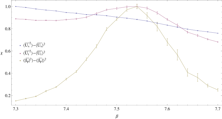
Unfortunately, our calculations indicate that the plaquette susceptibility has a weakly varying signal over the phase transition – too weak in fact to be useful on the lattice volumes that we are able to contemplate using. To show what happens it is convenient to partition the plaquettes into those that are only spatial $\overline{U}_{s}$ and those that have links in a temporal direction $\overline{U}_{t}$. Figure 1 shows the spatial plaquette susceptibility $\chi_{\overline{U}_{s}}$ and the temporal plaquette susceptibility $\chi_{\overline{U}_{t}}$ in the region of the phase transition for an $SO(4)$ $32^{2}3$ volume (renormalised for purposes of comparison). We need a clear peak in the susceptibility to identify the location of the phase transition but we see instead that $\chi_{\overline{U}_{s}}$ has no obvious peak structure while $\chi_{\overline{U}_{t}}$ has only a very weak peak structure. For other $SO(N)$ groups, we also typically find that $\chi_{\overline{U}_{s,t}}$ have no useful peak structures on the volumes we use. Of course when $L_{s}\to\infty$ the peaks should eventually appear and grow, but it does mean that for our purposes the plaquette susceptibility is not a useful order parameter.

An alternative order parameter is provided by the temporal Polyakov loop $l_{P}$. As described earlier, its expectation value has a direct relation to the free energy of an isolated charge, and it is therefore a natural order parameter for the deconfining transition. We shall shortly see that the Polyakov loop operator $\overline{l_{P}}$ has a much clearer signal in the region of the phase transition, compared to the plaquette operators. Around the transition it tunnels between confined and deconfined phases so that $\overline{l_{P}}$ takes discrete values with very small fluctuations around these. There is however a problem at finite $V$. If there is a non-trivial centre symmetry then tunnelling between the corresponding deconfined phases will cause ${\overline{l_{P}}}$ to average to zero for $T>T_{c}$. This is not an issue for $SO(2N+1)$ gauge theories since these have a trivial center symmetry, but it is a problem for $SO(2N)$ with its $\mathbb{Z}_{2}$ center symmetry. The same problem arises, of course, for $SU(N)$ gauge theories. The standard (if theoretically ugly) fix is to take the absolute value of the Polyakov loop after averaging it over the spatial volume

$$\left|\overline{l_{P}}\right|=\left|\frac{1}{L_{s}^{2}}\sum_{\mathbf{x}}l_{P}(\mathbf{x})\right|$$ (25)

and to use $\left|\overline{l_{P}}\right|$ as an order parameter and to construct an associated susceptibility from that,

$$\frac{\chi_{\left|\overline{l_{P}}\right|}}{L_{s}^{2}L_{t}}=\Braket{\left missing}{\overline{l_{P}}}{{}^{2}}-\Braket{\left missing}{\overline{l_{P}}}{}^{2}.$$ (26)

This has the disadvantage that $\Braket{\left missing}{\overline{l_{P}}}{}\neq 0$ in the confined phase as well as in the deconfined phase, but the values are very different and it has a very good signal in the region of the phase transition. We return to our $SO(4)$ $32^{2}3$ lattice in Figure 1, and plot the Polyakov loop susceptibility. We see that $\chi_{\left|\overline{l_{P}}\right|}$ has a much clearer peak structure than the plaquette susceptibilities shown in the same figure.

So, in a plot of $\Braket{\left missing}{\overline{l_{P}}}{}$ against $\beta$ in the neighbourhood of $\beta_{c}$, we would expect to see the value of $\Braket{\left missing}{\overline{l_{P}}}{}$ increase from near-zero to some non-zero value over a narrow range of $\beta$. For a first order transition this range shrinks to zero as the volume increases, becoming a discontinuity at $V=\infty$, while for a second order transition this range remains finite and there is no discontinuity, but the slope at $\beta_{c}$ tends to $\infty$. We show an example, obtained on a $20^{2}3$ lattice in $SO(6)$, in Figure 2. We expect to see a corresponding peak in $\chi_{\left|\overline{l_{P}}\right|}$ at $\beta_{c}$, as in Figure 1. For a first order transition, we expect the susceptibility $\chi_{\left|\overline{l_{P}}\right|}$ to approach a delta function singularity as $V\to\infty$. For a second order phase transition, we expect that the susceptibility $\chi_{\left|\overline{l_{P}}\right|}$ has a peak over a finite range of $\beta$ around $\beta_{c}$, with a cusp-like divergence at $\beta_{c}$.

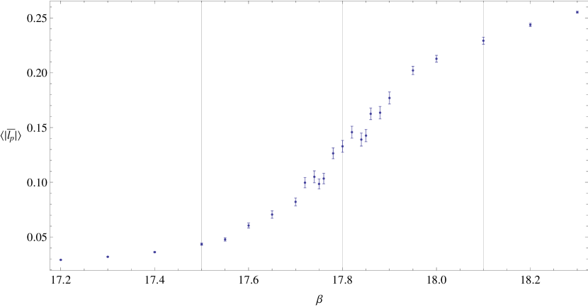
For odd $N$ there is no $Z_{2}$ symmetry to be spontaneously broken, so we can use our cleaner original variable, $\Braket{\overline{l_{P}}}$, to characterise the transition. In Fig.3 we plot this quantity against $\beta$ for a $48^{2}4$ lattice in $SO(7)$ with a sharp transition visible near the middle of the range. (Since the lattice spacing varies roughly as $1/\beta$, the range $\beta\in[20,40]$ corresponds roughly to the range $T/T_{c}\in[0.66,1.5]$.) Despite the lack of a centre symmetry, we find that for $\beta\leq 26.0$ our values are all consistent with $\Braket{\overline{l_{P}}}$ being zero within errors, with values $\sim\pm 10^{-5}$. This behaviour motivates describing the transition as being ‘deconfining’ even if the low-$T$ vacuum eventually turns out not to be exactly confining.

4.5 Tunnelling

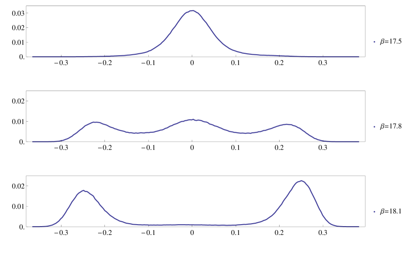
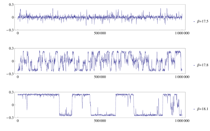
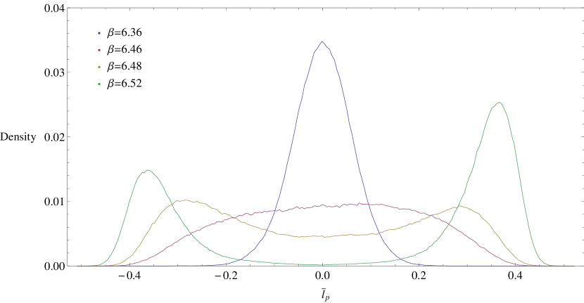
We can represent the values of $\overline{l_{P}}$ obtained from the sequence of field configurations generated at a given $\beta$ in a Monte Carlo run as either a histogram over the entire run, or as a history plot along the run. For $\beta<\beta_{c}$, we expect the theory to be confining so that $\Braket{\overline{l_{P}}}\approx 0$. On the histogram, we would expect that the values of $\overline{l_{P}}$ form a narrow peak around zero while, on the history plot, we would expect the values to fluctuate around zero. For $\beta>\beta_{c}$, the system would be in a deconfined phase so that $\Braket{\overline{l_{P}}}\neq 0$, and we would expect to see deconfined peaks at non-zero values on the histogram. For $SO(2N)$ gauge theories, we would expect to see two deconfined peaks at non-zero values, reflecting the spontaneous breaking of the $\mathbb{Z}_{2}$ center symmetry, while, for $SO(2N+1)$ gauge theories, where the center symmetry is trivial, we would only expect one deconfined peak at a non-zero value.

For a first order transition we would expect that as we increase $\beta$ towards $\beta\approx\beta_{c}$, and beyond, we should see deconfined peaks appear at non-zero values while the confined peak at zero decreases. And in a history plot we would see jumps that reflect tunnelling between the confined and deconfined phases. Beyond $\beta\approx\beta_{c}$ any tunnelling should be only between the two deconfined phases for even $N$, and no tunnelling for odd $N$. The behaviour for even $N$ is illustrated for $SO(6)$ on a $20^{2}3$ lattice in the histograms in Fig.4 and the history plots in Fig.5. For odd $N$ we illustrate the expected behaviour in $SO(7)$ on a $48^{2}4$ lattice in the history plot in Fig.6 and the histograms in Fig.7. The coexistence of both confining and deconfining peaks at a given $\beta$ establishes that we have a first order transition in both $SO(6)$ and $SO(7)$.

For a second order transition, there is no phase coexistence. As we increase $\beta$, we would expect the confined peak around zero to spread out and, once it disappears, the deconfined peaks emerge at $\beta=\beta_{c}$. On the history plot, we would expect to see significant fluctuations around zero for $\beta<\beta_{c}$ before the onset of tunnelling between the deconfined phases for $\beta>\beta_{c}$. This is illustrated for the case of a $28^{2}2$ lattice in $SO(4)$ in Figure 8.

Hence, we can use both the histograms and history plots of $\overline{l_{P}}$ to distinguish between first and second order transitions.

4.6 Identifying $\beta_{c}$

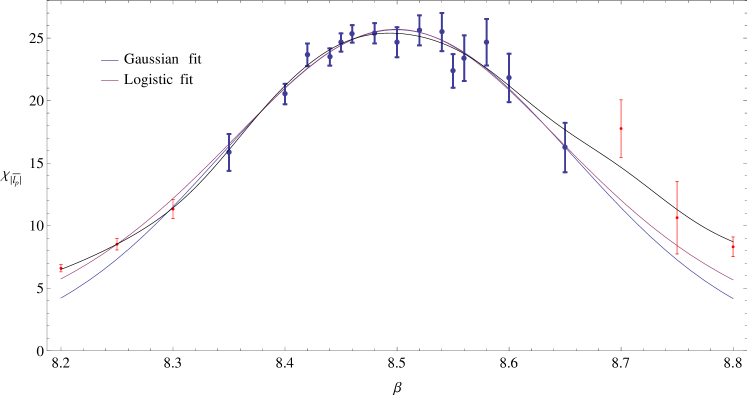
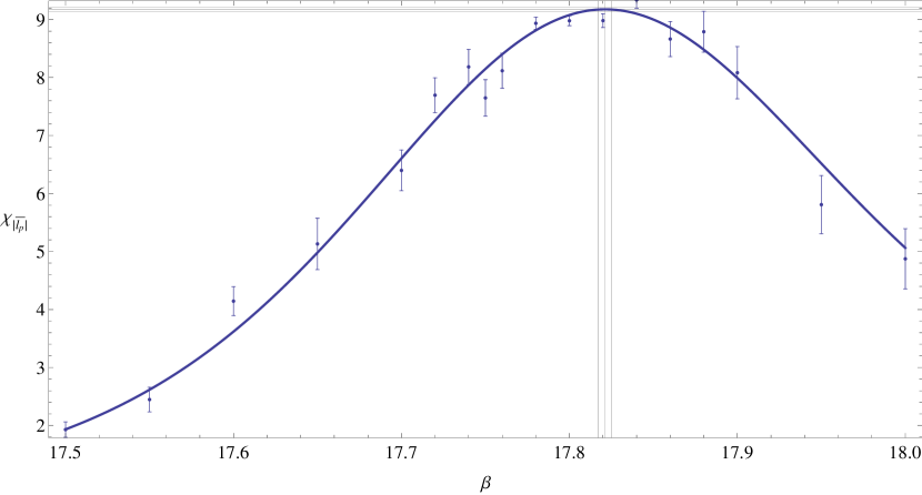
To calculate $\beta_{c}$ on a given volume $V$ we need to locate the maximum of the susceptibility. We do so by first performing separate runs at different $\beta$ values, and then doing more runs at values of $\beta$ near the peak. We use the standard density of states reweighting method Ferrenberg:1988nr ; Huang:1991lr to construct a smooth interpolating function through the measured values, whose maximum provides our estimate of $\beta_{v}c$ on the given volume $V$. For some very large spatial volumes, the values that arise in the reweighting algorithm exceed the machine precision. In principle this obstacle should be surmountable by some judicious alteration of the algorithm, but in these cases we choose instead to use curve fitting to find $\beta_{c}$, based on a logistic function for the Polyakov loop, which in practice turns out to have a comparable performance to that of our reweighting algorithm, as we see from Fig.9 and Table 1.

5 $SO(N)$ lattice calculations in $D=2+1$

We generate sequences of lattice field configurations using an $SO(N)$ adaptation of the $SU(N)$ Cabbibo-Marinari heat bath algorithm Cabibbo1982387 , which we describe in our companion paper on the $SO(N)$ spectrum, Lau:aa . We use the plaquette action in eqn(11).

We express the deconfining temperature in physical units by calculating suitable mass scales $\mu$ of the gauge theories at $T=0$ and then taking ratios $aT_{c}/a\mu=T_{c}/\mu$, which we can then extrapolate to the continuum limit in a standard way. Three such quantities are the string tension, coupling, and lightest scalar glueball mass (the mass gap). We now briefly describe how we calculate these on the lattice. We provide fuller details in Lau:aa .

5.1 String tensions

To obtain the string tension, we calculate the energy $E(l)$ of the lightest flux tube that winds around the spatial torus of size $l$ on a lattice that corresponds to $T\sim 0$. To do this, we use correlators of zero-momentum sums of Polyakov loop operators, that have been ‘blocked’ to obtain a very good overlap onto the ground state Teper1987345 supplemented by a standard variational calculation Teper:1998rw . We expect that $E(l)\rightarrow\sigma l$ for $l$ large Lau:aa . For finite $l$, we expect $E(l)$ to be well-approximated by Athenodorou:2011hl ; Aharony ; Dubovsky

$$E(l)=\sigma l\left(1-\frac{\pi}{3\sigma l^{2}}\right)^{\frac{1}{2}}.$$ (27)

By evaluating the string tension at $\beta_{c}$, we can then express the deconfining temperature in the dimensionless ratio $T_{c}/\surd\sigma$.

5.2 Couplings

In $D=2+1$ the coupling $g^{2}$ provides a mass scale for the theory. In the continuum limit

$$\lim_{\beta\to\infty}\frac{\beta}{2N^{2}}=\frac{1}{ag^{2}N}$$ (28)

where $g^{2}N$ is the ’t Hooft coupling which one keeps constant as $N$ increases in order to have a smooth large-$N$ limit. At finite lattice spacing the coupling is scheme dependent, and in that sense not a physical quantity, but different choices of coupling differ at $O(ag^{2})$ and so converge to the same continuum limit. It makes sense to try and choose a coupling scheme within which that convergence is rapid. Previous calculations in $D=2+1$ $SU(N)$ Teper:1998rw have found it useful to employ the mean field improved coupling Lepage:1993dp

$$\beta_{I}=\beta\Braket{\frac{1}{N}\text{tr}(U_{p})}.$$ (29)

We will choose to use this improved coupling to calculate the continuum value of $T_{c}/g^{2}N$.

5.3 Scalar glueball masses

$SO(N)$ gauge theories have a glueball mass spectrum similar to that in $SU(N)$ gauge theories, except that all glueballs have charge conjugation $C=+$. The lightest glueball has spin $J=0$ and parity $P=+$ and it is the glueball mass that we can calculate most accurately. We evaluate the continuum glueball masses $M_{0^{+}}/\surd\sigma$ in Athenodorou:2015aa ; Lau:aa and use these values as another way of expressing the deconfining temperature in physical units $T_{c}/M_{0^{+}}=T_{c}/\surd\sigma\times\surd\sigma/M_{0^{+}}$.

6 Results: infinite volume limits

6.1 Methodology

We need to calculate $\beta_{c}(V\rightarrow\infty)$ on our $L_{s}^{2}L_{t}$ lattices, to obtain the lattice deconfining temperature $T_{c}=1/a(\beta_{c}(V=\infty))L_{t}$. Using $\left|\overline{l_{P}}\right|$ as our order parameter, for a given finite spatial volume $V$, we calculate $\beta_{c}(V)$ by calculating the susceptibility $\chi_{\left|\overline{l_{P}}\right|}$ for a range of $\beta$ values, reweighting the data from those $\beta$ values where we observe there to be tunnelling between the confined and deconfined phases, and then locating the maximum. If the lattice volume is too large for our reweighting algorithm, we follow the curve fitting procedure mentioned above. Then $\beta_{c}(V)$ is the $\beta$ value that corresponds to a maximum in $\chi_{\left|\overline{l_{P}}\right|}$. This is illustrated in Fig. 10 on a $20^{2}.3$ lattice in $SO(6)$ where we see that the reweighted curve agrees well with our original data and that the estimates for $\beta_{c}$ and $\chi_{\left|\overline{l_{P}}\right|}(\beta_{c})$ have very small errors.

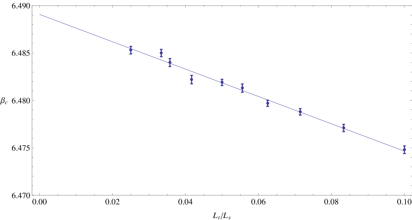
Repeating this calculation for a range of $V$ we can extrapolate to $V=\infty$ using the finite size scaling formulae in eqn(22). In Figure 11 we display such an infinite volume extrapolation for a second order transition in $SO(4)$ with $L_{t}=2$, and in Figure 12 for a first order transition, in $SO(16)$ with $L_{t}=3$. In both cases we see that the extrapolation is precise and well-defined. As will be apparent when we list the results of our extrapolations, this is mostly the case, albeit with a significant number of exceptions where the fits are statistically poor .

Since the tunnelling in a first order transition is important to both identifying and locating the transition, it is useful to consider how this tunnelling varies with $V$ and $N$. Using a standard argument, the tunnelling must proceed through an intermediate configuration where the two phases are separated by two spatial domain walls of length $l_{s}=aL_{s}$, with a probability of

$$P_{W}(T)\propto\text{exp}\left(-\frac{2\sigma_{W}l_{s}}{T}\right)=\text{exp}\left(-2a^{2}\sigma_{W}L_{s}L_{t}\right)$$ (30)

relative to the probability of a single phase at the same temperature. Here $\sigma_{W}$ is the surface tension per unit length of the domain wall. (All this assumes that our Monte Carlo is a local process. If we have global updates, which are trivial to construct between the two deconfined phases, then this discussion will need changing.) Now just as in $SU(N)$ we expect the surface tension to grow with $N$ as $\sigma_{W}\propto N^{2}$ Lucini:2004fk . Hence, the probability of the domain walls and the probability of tunnelling decreases exponentially as either the volume $V$ or as $N$ increase. Thus transitions between the two states are increasingly rare at large $V$, especially at large $N$, and this provides an effective upper bound on the volumes we can consider at a given $N$. In addition to this, critical slowing down will also suppress the frequency of tunnelling as $a(\beta_{c})$ decreases.

Since the accuracy of our calculation of $\beta_{c}(V)$ depends primarily on the number of tunnelling fluctuations, rather than the fluctuations within a given phase, we should, ideally, use errors in our reweighting procedure derived solely from the number of tunnellings. Since this is not straightforward to do, we instead used only data points from runs that clearly have tunnellings, but then used ‘naive’ errors, albeit based on large bin-sizes each of which would usually contain some tunnellings. While we believe this ‘fix’ is usually reliable, it nonetheless leaves a systematic error in our calculations which we only partially control, and this may be the reason for the very poor goodness of fit of a few of our $V\to\infty$ extrapolations.

6.2 $SO(4)$ and $SO(5)$

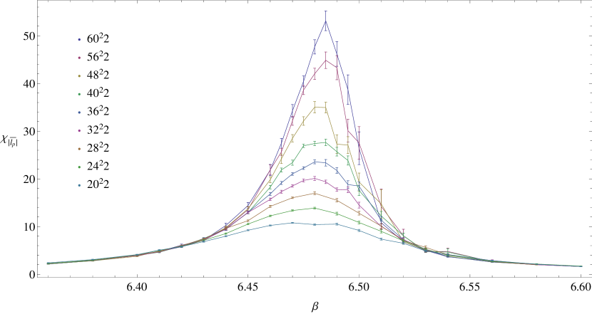
The $SO(4)$ and $SO(5)$ deconfining phase transitions are second order. We can see this from the ${\overline{l_{P}}}$ histograms, such as Figure 8, which show a continuous transition from confined to deconfined phases as we increase $\beta$. We can also see this in susceptibility plots for different spatial volumes at fixed $L_{t}$, such as Figure 13, which show that, as the spatial volume increases, the susceptibility peak height increases, and the large volume susceptibility provides an envelope for the ones at smaller $V$.

For $SO(4)$, we can use reweighting for $2\leq L_{t}\leq 4$ to calculate $\beta_{c}$. For $L_{t}=5$, the susceptibility peak is at $\beta\in[9.0,10.0]$. This is in the region of the ‘bulk’ transition which separates weak and strong coupling and which we will discuss later, and which affects the data so greatly that reweighting does not work. For $L_{t}\geq 6$, the spatial volumes become so large that we cannot reweight the data using our standard algorithm and so we curve fit instead. For smaller $L_{t}$, the values lie on a smooth curve with small errors and the reweighted values fit well with the original data. At larger $L_{t}$, the data is more scattered than at smaller $L_{t}$, although we can still estimate $\beta_{c}$ with usefully small errors. We present the $SO(4)$ values of $\beta_{c}(V)$ for volumes $V$ with $L_{t}=2,3,4,6,7,8,10,12$ in Tables 2 and 3.

To extrapolate $\beta_{c}(V\rightarrow\infty)$ to the infinite volume limit using eqn(22), we need a value for the critical exponent $\nu$. We recall that the Svetitsky-Yaffe conjecture Svetitsky1982423 puts the deconfining phase transition in the same universality class as the order/disorder transition of the spin system which is in the same spatial dimensions and which is invariant under the group that corresponds to the centre of the gauge group. For $SO(2N)$ gauge groups, which have a $\mathbb{Z}_{2}$ centre symmetry, this puts the deconfining phase transition in the same universality class as the $D=2$ Ising model. In the case of $SO(4)\sim SU(2)\times SU(2)$ we would expect the deconfining phase transition to be in the universality class of two decoupled $D=2$ Ising models. In the case of $SO(5)$, we know that $Sp(2)$ forms the vector representation of $SO(5)$, which also has a $\mathbb{Z}_{2}$ centre symmetry so we would expect that its deconfining phase transition should also be in the universality class of the $D=2$ Ising model Pepe:2004 . Since the order/disorder transition for the $D=2$ Ising model has critical exponents

$$\gamma=1.75\quad;\quad\nu=1$$ (31)

we expect these to be the critical exponents of the $SO(4)$ and $SO(5)$ deconfining phase transitions. One can try to support this choice by fitting $\nu$ to our actual data, but because the variation of $\beta_{c}(V)$ is weak one needs a large lever arm in $V$, and very accurate data, to get a useful result. With our data the only useful fit for $\nu$ is to the $SO(4)$ $L_{t}=2$ data from which we obtain the estimate $\nu=0.88(19)$, which provides some support for the universality based value, which we shall employ from now on.

We list the resulting $SO(4)$ $\beta_{c}(V=\infty)$ values in Table 4 showing in each case the goodness of fit as measured by the value of $\bar{\chi}^{2}_{\text{dof}}$ (chi-squared divided by the number of degrees of freedom). We see that the extrapolated values have small errors and most of the $\bar{\chi}^{2}_{\text{dof}}$ values are reasonable. (One $\bar{\chi}^{2}_{\text{dof}}$ value is very large, and this is due to a scatter among values with very small errors, which cannot be remedied by dropping values at the smallest $V$.)

For $SO(5)$, we can use reweighting for $2\leq L_{t}\leq 6$ and curve fitting for $L_{t}\geq 7$ to calculate $\beta_{c}$. Since the centre symmetry is trivial we cannot use that to argue that $\Braket{\overline{l_{P}}}\approx 0$ in the low $T$ confined phase. However, our calculations show that this is indeed the case. We list the $\beta_{c}(V)$ values for $SO(5)$ with $L_{t}=2,3,4,5,6,7,8,10$ in Table 5 and for the infinite volume limits in Table 6. We see that the extrapolated values again have small errors and that the $\bar{\chi}^{2}_{\text{dof}}$ values are mostly reasonable.

6.3 $SO(6)$

The $SO(6)$ deconfining phase transition is (weakly) first order: the coexisting phases are apparent, as in Figure 4, but are less well defined than for $SO(N\geq 7)$. While susceptibility plots indicate that the transition has features from both first and second order transitions, the ${\overline{l_{P}}}$ histograms (such as Figure 4) show a clear first order phase coexistence. We extrapolate to the infinite volume limit using eqn(22). We list the $\beta_{c}(V)$ values in Table 7 and the infinite volume limits in Table 8.

6.4 $SO(7)$, $SO(8)$, $SO(9)$, $SO(12)$, and $SO(16)$

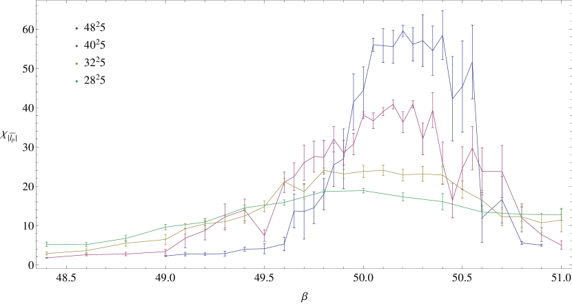
The $SO(N\geq 7)$ deconfining phase transitions are all first order, as is clear from the phase coexistence in the $\Braket{\overline{l_{P}}}$ histograms and from the susceptibility plots (such as Figure 14) which show the whole peak shrinking and its height growing as $V$ increases. For $SO(7)$ and $SO(9)$ our calculations show that, just as for $SO(5)$, we have $\Braket{\overline{l_{P}}}\approx 0$ despite the absence of a non-trivial center symmetry.

We list the $\beta_{c}(V)$ values in Tables 9, 11, 13, 15, and 17 and the infinite volume limits, obtained using eqn(22), in Tables 10, 12, 14, 16, and 18.

7 Results: continuum limits

7.1 Methodology

To extrapolate $T_{c}$ to the continuum limit, i.e. $a\rightarrow 0$ or equivalently $\beta\rightarrow\infty$, we express $T_{c}$ in units of some other energy scale $\mu$, calculated at the same value of $\beta$, and extrapolate the resulting dimensionless ratio $\lim_{\beta\to\infty}T_{c}/\mu$. For the scale $\mu$ we will use either the string tension, $\mu=\surd\sigma$, calculated at $\beta_{c}$ and at $T\approx 0$, or the ’t Hooft coupling, $\mu=g^{2}N$.

Let us express the critical temperature in units of the string tension evaluated at the critical coupling $\beta_{c}$ on a lattice corresponding to $T\simeq 0$,

$$\frac{T_{c}}{\surd\sigma}(a)=\frac{1}{a(\beta_{c})\surd\sigma L_{t}}.$$ (32)

Once we have $T_{c}/\surd\sigma$ for each of our values of $L_{t}$, we take the continuum limit $a\rightarrow 0$. Since this is the ratio of two physical mass scales, we expect the leading correction to be $\mathcal{O}(a^{2})$ Symanzik:1983uq ,

$$\frac{T_{c}}{\surd\sigma}(a)=\frac{T_{c}}{\surd\sigma}(a=0)+ca^{2}\sigma(a)+\cdots$$ (33)

for some constant $c$.

We can similarly express the critical temperature in terms of the ’t Hooft coupling,

$$\frac{T_{c}}{g^{2}N}\equiv\frac{aT_{c}}{ag^{2}N}=\frac{\beta_{c}}{2N^{2}}\frac{1}{L_{t}}.$$ (34)

As remarked earlier, at finite $\beta$ the lattice coupling is scheme dependent, and we will choose to use the mean field improved coupling, replacing $\beta$ by $\beta_{I}=\beta\Braket{\frac{1}{N}\text{tr}(U_{p})}$ in the above. Once we have $T_{c}/(g^{2}N)$ for each of our $L_{t}$ values, we can take the continuum limit

$$\frac{T_{c}}{g^{2}N}(a)=\frac{T_{c}}{g^{2}N}(a=0)+cag^{2}N+\cdots$$ (35)

where the leading order correction is $\mathcal{O}(a)$ rather than $\mathcal{O}(a^{2})$ since, unlike the string tension or glueball mass, the lattice coupling is not a physical quantity.

We note that the errors on the values of $\beta_{c}$ and $\beta_{I,c}$ are typically much smaller than on the $a\surd\sigma$ lattice values. However this greater accuracy is offset by the fact that these values are ‘further away’ from the continuum limit in that the leading correction is $O(a)$ rather than $O(a^{2})$. Moreover one would naively expect $T_{c}$ and $\sigma$ to be more closely correlated than $T_{c}$ and some lattice $g^{2}$, and so their ratio to be closer to its continuum value. For this reason we will place more stress on our continuum extrapolation of $T_{c}/\surd\sigma$ than on $T_{c}/g^{2}N$.

Finally we remark that we could equally well express the critical temperature in units of the lightest scalar glueball mass $m_{0^{+}}$, by calculating this mass at each $\beta_{c}$ in the $T\simeq 0$ theory, and extrapolating the resulting dimensionless ratio to the continuum limit. However we do not do this here. Rather we simply obtain the continuum ratio $T_{c}/m_{0^{+}}$ from the continuum limit of $m_{0^{+}}/\surd\sigma$ calculated in Lau:aa and our extrapolated value of $T_{c}/\surd\sigma$,

$$\frac{T_{c}}{m_{0^{+}}}=\frac{T_{c}/\surd\sigma}{m_{0^{+}}/\surd\sigma}.$$ (36)

7.2 Bulk transition

Lattice gauge theories generally have some kind of ‘bulk’ transition between the regions of strong and weak coupling, where the coupling expansion changes from powers of $\beta\propto 1/(ag^{2})$ to powers of $1/\beta\propto ag^{2}$. Since an extrapolation to the continuum limit, $\beta\to\infty$, is only plausible, a priori, if made using values obtained in the weak coupling region, it is important to know where this bulk transition occurs.

With the $SO(N)$ plaquette action, we find that the bulk transition seems to be characterised by the appearance of a very light excitation in the scalar glueball sector, with the rest of the glueball spectrum being essentially unaffected. Moreover we find that the visibility of this light excitation is sensitive to the lattice volume and that as $N$ increases, we can use smaller volumes to identify the bulk transition in this way. This is an interesting and unusual transition, which we will describe in greater detail in our companion paper on the glueball spectrum Lau:aa . For our present purposes, we only need to note that it provides an unambiguous way to identify the location of the bulk transition. We show the $\beta$ values corresponding to this bulk transition in Table 19 together with the range of $L_{t}$ values for which the corresponding $\beta_{c}$ lie in the weak coupling region. We note that the transition moves to weaker coupling as $N$ decreases, making the weak coupling calculations more expensive at small $N$. This is why we have not performed $SO(3)$ calculations, which one can estimate would necessitate using $L_{t}>10$ (and up to $L_{t}\sim 20$ to have a useful lever arm for a continuum extrapolation).

To calculate the continuum limit of the deconfinement temperature, we shall use data corresponding to values in the weak coupling region, ignoring the data from $L_{t}$ values that have $\beta_{c}$ values in the strong coupling region. Occasionally, where the would-be susceptibility peak around $\beta_{c}$ overlaps with this bulk transition, it may be grossly distorted by the very light scalar excitation (which can also affect the winding flux tube spectrum) and we are then unable to obtain a usefully precise value of $\beta_{c}$.

7.3 $SO(4)$

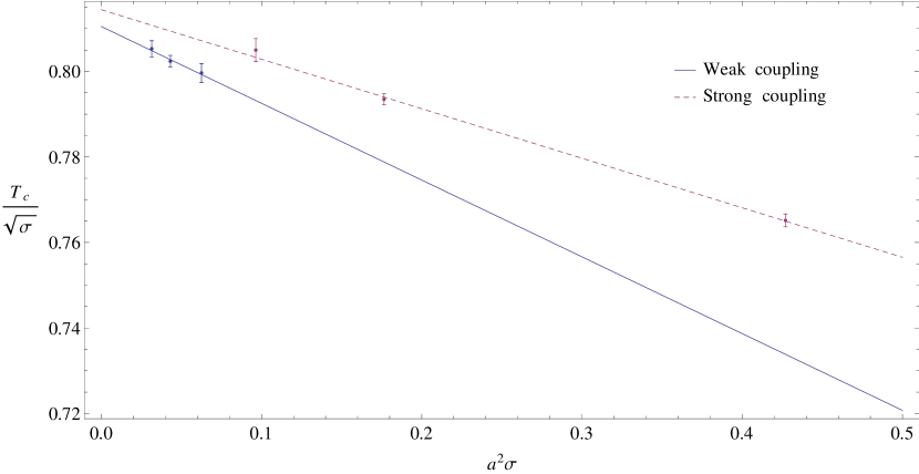
For $SO(4)$, the $\beta_{c}$ values for $L_{t}<5$ are in the strong coupling region whereas the $\beta_{c}$ values for $L_{t}>5$ are in the weak coupling region. The deconfining transition for $L_{t}=5$ mixes with the bulk transition and we do not attempt to extract corresponding values of $\beta_{c}$. We give the corresponding values of $T_{c}/\surd\sigma$ in Table 20.

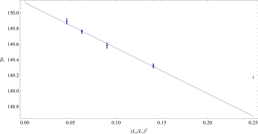
We extrapolate the values of $T_{c}/\surd\sigma$ to the continuum limit using eqn(33). We display the data and the fits in Figure 15. There are two separate fits on display. The first is to the weak-coupling data, obtained on lattices with $L_{t}\geq 6$. This data shows very little dependence on $a$ and the fit with just the leading $O(a^{2})$ correction works well. This is no surprise because $a^{2}\sigma\ll 1$ for all the weak coupling data. We obtain a continuum limit

$$\frac{T_{c}}{\surd\sigma}(a=0)=0.7702(88)\quad\bar{\chi}^{2}_{\text{dof}}=0.12\quad SO(4)\text{ (weak coupling)}.$$ (37)

The second fit is motivated by the fact that the three strong coupling values obtained on lattices with $L_{t}\leq 4$, appear to lie on a stright line. A linear fit as in eqn(33) works well and provides us with what we dub a ‘strong coupling’ continuum limit

$$\frac{T_{c}}{\surd\sigma}(a=0)=0.8638(21)\quad\bar{\chi}^{2}_{\text{dof}}=0.09\quad SO(4)\text{ (strong coupling)}.$$ (38)

This linearity of the strong coupling data is unexpected and indeed bizarre. It may just be an accident, in which case our exercise is meaningless. However it may be that $a^{2}$ is small enough for the operator expansion of the lattice action in powers of $a^{2}$ is viable even if the coupling expansion in powers of $1/\beta$ is not. If so one might speculate that this provides some kind of strong coupling continuum limit. In any case, the true continuum limit of the $SO(4)$ theory is the one extracted from the weak coupling values in eqn(37).

Similarly, we can calculate the critical temperatures in units of the ’t Hooft coupling. The values of $T_{c}/(g^{2}N)$ are listed in Table 20. We can plot $T_{c}/(g^{2}N)$ against $ag^{2}N$ and extrapolate to the continuum limit using eqn(35). The continuum limit is

$$\frac{T_{c}}{g^{2}N}(a=0) =0.04567(43) \bar{\chi}^{2}_{\text{dof}}=2.17 SO(4)\text{ (weak coupling)}$$ (39)

where we need to drop the $L_{t}=6$ point from the fit in order to obtain a reasonable $\bar{\chi}^{2}_{\text{dof}}$ with just a leading order weak coupling correction. (Note that the strong coupling values do not fit onto a linear extrapolation in $1/\beta_{I}$, which is of course as expected.)

Finally, we express the critical temperature in units of the lightest scalar glueball mass $M_{0^{+}}$. We use the continuum value of $M_{0^{+}}/\surd\sigma$ calculated in Lau:aa with our above continuum value of $T_{c}/\surd\sigma$ to obtain

$$\frac{T_{c}}{M_{0^{+}}}(a=0)=0.2293(30)\qquad SO(4)\text{ (weak coupling)}.$$ (40)

7.4 $SO(5)$ and $SO(6)$

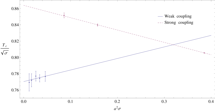
For both $SO(5)$ and $SO(6)$, the $\beta_{c}$ values for $L_{t}\geq 5$ are in the weak coupling region and so can be used for a continuum extrapolation. To obtain the critical temperature in string tension units $T_{c}/\surd\sigma$, we calculate the string tension at each $\beta_{c}$ as in $SO(4)$. We list the resulting values for $SO(5)$ in Table 21 and for $SO(6)$ in Table 22. We display the continuum extrapolation for $SO(6)$ in Figure 16.

In the case of $SO(5)$, unlike $SO(4)$, there were difficulties in using a linear extrapolation in the weak coupling region due to peculiar variation in the value of $T_{c}/\surd\sigma$. To obtain a good fit we had to drop the two smallest $L_{t}$ points in the weak coupling region. (Context: for no other $N$ did we need to drop any weak coupling points.) $SO(5)$ is the largest $SO(N)$ group for which the transition is second order and it might be that this is behind this atypical behaviour. The continuum limit from within the weak coupling region is

$$\frac{T_{c}}{\surd\sigma}(a=0) =0.7963(114), \bar{\chi}^{2}_{\text{dof}}=0.003 SO(5).$$ (41)

We also note that the strong coupling values fit less well with a linear extrapolation than they did for $SO(4)$, giving a strong coupling ‘continuum’ extrapolation of $T_{c}/\surd\sigma=0.783(4)$ with a mediocre $\bar{\chi}^{2}_{\text{dof}}=2.78$.

$SO(6)$ is the smallest group for which the transition is first order. The continuum limit taken from data within the weak coupling region is

$$\frac{T_{c}}{\surd\sigma}(a=0) =0.8105(42), \bar{\chi}^{2}_{\text{dof}}=0.16 SO(6).$$ (42)

There is also a good linear extrapolation using the strong coupling values that gives $T_{c}/\surd\sigma=0.8144(20)$ with $\bar{\chi}^{2}_{\text{dof}}=0.59$. We note that here the strong coupling extrapolation is consistent with the true weak-coupling continuum limit.

We can also calculate the critical temperatures in units of the coupling. $T_{c}/(g^{2}N)$. The values are listed in Table 21 and Table 22. We can then plot $T_{c}/(g^{2}N)$ against $ag^{2}N$ and extrapolate to the continuum limit using eqn(35). The continuum limits, from within the weak coupling regions, are

$$\left.\frac{T_{c}}{g^{2}N}\right|_{a=0}=\begin{cases}0.05544(92)\quad\bar{\chi}^{2}_{\text{dof}}=0.05\quad SO(5)&\\ 0.05996(19)\quad\bar{\chi}^{2}_{\text{dof}}=0.53\quad SO(6)&\end{cases}.$$ (43)

In the case of the $SO(5)$ data, the points seem to lie on a smooth curve and do not exhibit the peculiar variation seen in the corresponding $T_{c}/\surd\sigma$ values.

Finally, we can calculate the critical temperatures in units of the lightest scalar glueball. Using the values of $M_{0^{+}}/\surd\sigma$ from Lau:aa we obtain

$$\left.\frac{T_{c}}{M_{0^{+}}}\right|_{a=0}=\begin{cases}0.2244(33)\quad SO(5)&\\ 0.2232(14)\quad SO(6)&\end{cases}.$$ (44)

7.5 $SO(7)$, $SO(8)$, $SO(9)$, $SO(12)$, and $SO(16)$

For $SO(7)$ and $SO(8)$ the $\beta_{c}$ values are in the weak coupling region for $L_{t}\geq 4$, and for $SO(9)$, $SO(12)$, and $SO(16)$ they are in the weak coupling region for $L_{t}\geq 3$.

We list the critical temperature values in string tension units $T_{c}/\surd\sigma$ for these groups in Tables 23, 24, 25, 26, and 27. The continuum limits are

$$\left.\frac{T_{c}}{\surd\sigma}\right|_{a=0}=\begin{cases}0.8351(38)\quad\bar{\chi}^{2}_{\text{dof}}=0.98\quad SO(7)&\\ 0.8418(39)\quad\bar{\chi}^{2}_{\text{dof}}=0.05\quad SO(8)&\\ 0.8515(14)\quad\bar{\chi}^{2}_{\text{dof}}=0.30\quad SO(9)&\\ 0.8642(38)\quad\bar{\chi}^{2}_{\text{dof}}=0.02\quad SO(12)&\\ 0.8780(38)\quad\bar{\chi}^{2}_{\text{dof}}=0.15\quad SO(16)&\end{cases}.$$ (45)

We note that all these fits are very good.

Similarly, we can calculate the critical temperature in units of the coupling, as listed in Tables 23, 24, 25, 26, and 27. We can then plot $T_{c}/(g^{2}N)$ against $ag^{2}N$ and extrapolate to the continuum limit using eqn(35). These plots have very similar forms to the corresponding $T_{c}/\surd\sigma$ plots. The continuum limits are

$$\left.\frac{T_{c}}{g^{2}N}\right|_{a=0}=\begin{cases}0.06478(18)\quad&\bar{\chi}^{2}_{dof}=4.01\quad SO(7)\\ 0.06809(16)\quad&\bar{\chi}^{2}_{dof}=0.00\quad SO(8)\\ 0.07043(7)\quad&\bar{\chi}^{2}_{dof}=0.10\quad SO(9)\\ 0.07552(14)\quad&\bar{\chi}^{2}_{dof}=0.63\quad SO(12)\\ 0.07947(17)\quad&\bar{\chi}^{2}_{dof}=0.85\quad SO(16)\end{cases}.$$ (46)

We can see that these continuum extrapolations are mostly good. (Given there is only one degree of freedom, the $SO(7)$ fit is not unacceptable.)

Finally, we can calculate the critical temperatures in units of the lightest scalar glueball mass $M_{0^{+}}$. Using the values for $N=7,8,12,16$ calculated in Lau:aa (there is no calculation for $N=9$) we find

$$\left.\frac{T_{c}}{M_{0^{+}}}\right|_{a=0}=\begin{cases}0.2234(12)\quad SO(7)&\\ 0.2224(15)\quad SO(8)&\\ 0.2217(18)\quad SO(12)&\\ 0.2220(22)\quad SO(16)&\end{cases}.$$ (47)

8 Results: large-$N$ limits

8.1 Deconfining temperature

In contrast to $SU(N)$, the leading large-$N$ correction for $SO(N)$ gauge theories is expected to be $\mathcal{O}(1/N)$. So we expect

$$\left.\frac{T_{c}}{\mu}\right|_{SO(N)}\stackrel{{\scriptstyle N\to\infty}}{{=}}\left.\frac{T_{c}}{\mu}\right|_{SO(\infty)}+\frac{c}{N}+\cdots$$ (48)

with $\mu$ a physical mass scale such as $\surd\sigma$, $m_{0^{+}}$ or $g^{2}N$.

Since one of our aims is to compare the values of $T_{c}$ for $SO(2N)$ and $SO(2N+1)$ gauge theories, it would be useful to have an estimate of $T_{c}$ in $SO(3)$. Since the $SO(3)$ and $SU(2)$ groups have the same Lie algebra, it is plausible to assume that they share the same value of $T_{c}/M_{0^{+}}$, where $M_{0^{+}}$ is the mass of the lightest scalar glueball. We have to be more careful with $T_{c}/\surd\sigma$ because the fundamental string tension in $SO(3)$ corresponds to the adjoint in $SU(2)$. Now, we know that in $SU(2)$ $T_{c}/\surd\sigma=1.1238(88)$ Jack-Liddle:2008xr We also know that in $SU(2)$ $M_{0^{+}}/\surd\sigma=4.7367(55)$ Athenodorou:aa and in $SO(3)$ $M_{0^{+}}/\surd\sigma=2.980(24)$ Lau:aa . From the ratio of these two numbers we extract an estimate of the ratio of fundamental string tensions in $SU(2)$ and $SO(3)$. All this implies that the $SO(3)$ continuum deconfining temperature in units of the string tension is

$$\frac{T_{c}}{\surd\sigma} =0.7072(80) SO(3).$$ (49)

We also know the $SO(3)$ string tension $\surd\sigma/(g^{2}N)=0.04576(36)$ Lau:aa , which tells us that

$$\frac{T_{c}}{g^{2}N} =0.03236(45) SO(3).$$ (50)

Finally, we can also infer from the above that the $SO(3)$ continuum deconfining temperature in units of the lightest scalar glueball mass is

$$\frac{T_{c}}{M_{0^{+}}} =0.2373(33) SO(3).$$ (51)

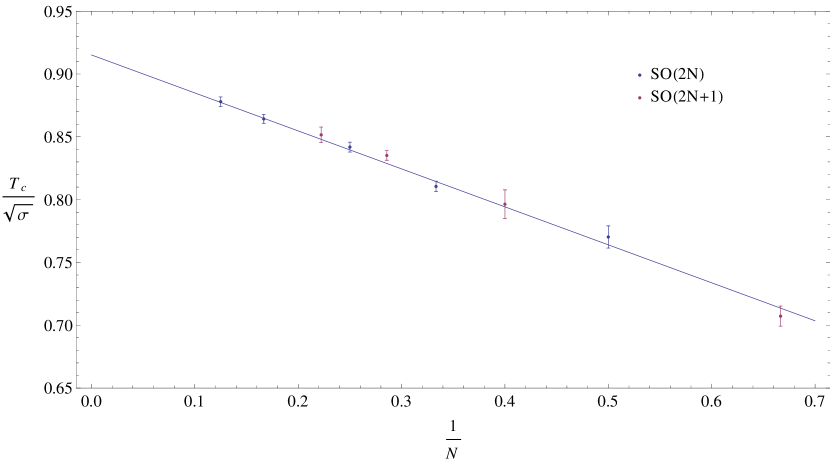
We list the $SO(N)$ deconfining temperatures in string tension units in Table 28. We begin by applying a linear fit in $1/N$ to just the $SO(2N)$ values. We do so for two reasons. Firstly, we intend to compare this limit to the $SU(N)$ large-$N$ limit motivated by the large-$N$ orbifold equivalence. Secondly, $SO(2N+1)$ has a different centre to $SO(2N)$, so the deconfinement properties might differ between the two sets of gauge theories and it is interesting to see if this is the case. In Figure 17 we plot all our values of ${T_{c}}/{\surd\sigma}$, including that inferred for $SO(3)$, against $1/N$, and we also show the best leading-order fit to just the $SO(2N)$ values. We see that the linear fit is very good. We also see that values for the $SO(2N+1)$ groups are consistent with lying on this fit. Indeed if we take all the values, including $SO(3)$, we obtain a very similar best fit:

$$\left.\frac{T_{c}}{\surd\sigma}\right|_{N\rightarrow\infty}=\begin{cases}0.9152(48)\quad\bar{\chi}^{2}_{\text{dof}}=0.58\quad SO(2N\geq 4)&\\ 0.9231(45)\quad\bar{\chi}^{2}_{\text{dof}}=0.52\quad SO(2N+1\geq 3)&\\ 0.9194(33)\quad\bar{\chi}^{2}_{\text{dof}}=0.82\quad SO(N\geq 3)&\end{cases}.$$ (52)

We conclude that at our level of accuracy there is no evidence for any difference in the way $T_{c}/\surd\sigma$ varies with $N$ in $SO(2N)$ and $SO(2N+1)$ gauge theories: the lack of a center symmetry in the latter appears to play no role. We also observe that the groups with a second order transition, $SO(N\leq 5)$, fall nicely on the smooth curve that describes the $N$-dependence of the first-order transitions, $SO(N\geq 6)$.

We can repeat the above, replacing $\surd\sigma$ by the ’t Hooft coupling $g^{2}N$. We list the $SO(N)$ deconfining temperatures in units of $g^{2}N$ in Table 28. To fit to all the values of $N$, we need to include an additional $O(1/N^{2})$ correction and, to avoid a systematic bias, we do the same for our separate fits to odd and even $N$. We find:

$$\left.\frac{T_{c}}{g^{2}N}\right|_{N\rightarrow\infty}=\begin{cases}0.09139(49)\quad\bar{\chi}^{2}_{\text{dof}}=2.53\quad SO(2N\geq 4)&\\ 0.09039(63)\quad\bar{\chi}^{2}_{\text{dof}}=0.43\quad SO(2N+1\geq 3)&\\ 0.09160(35)\quad\bar{\chi}^{2}_{\text{dof}}=1.45\quad SO(N\geq 3)&\end{cases}.$$ (53)

We see that values of $T_{c}/(g^{2}N)$ obtained for the $SO(2N+1)$ groups are consistent with those for $SO(2N)$.

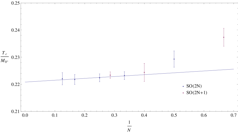
Finally, we list the $SO(N)$ deconfining temperatures in units of the lightest scalar glueball mass in Table 28 and plot these values in Figure 18. We show a leading-order fit to $SO(2N)$ for $2N\geq 6$ since the data (if one pays attention to the $SO(3)$ value) indicates the need for a higher order correction at the lower values of $N$. We do not fit odd $N$ separately because we do not have available a glueball mass for $SO(9)$, and so the number of odd $N$ values is too small to fit. We also perform fits with an additional $O(1/N^{2})$ correction to both $SO(2N\geq 4)$ and to all our values, $SO(N\geq 3)$. Altogether, these fits give:

$$\left.\frac{T_{c}}{M_{0^{+}}}\right|_{N\rightarrow\infty}=\begin{cases}0.2209(28)\quad\bar{\chi}^{2}_{\text{dof}}=0.03\quad SO(2N\geq 6)&\\ 0.2189(23)\quad\bar{\chi}^{2}_{\text{dof}}=0.51\quad SO(2N\geq 4)&\\ 0.2230(39)\quad\bar{\chi}^{2}_{\text{dof}}=0.10\quad SO(N\geq 3)&\end{cases}.$$ (54)

We note that the linear fit is particularly flat compared to the linear fit in Figure 17 and the one to ${T_{c}}/{g^{2}N}$. Finally, we again see evidence that the $SO(2N)$ and $SO(2N+1)$ values form a single smooth series.

8.2 Large-$N$ scaling

We have assumed throughout that the large-$N$ limit requires keeping $g^{2}N$ fixed and that the leading correction is $O(1/N)$, guided by the all-orders analysis of diagrams Lovelace:1982fk . Certainly, keeping $g^{2}N$ fixed is necessary if one wants to obtain an $SO(\infty)$ theory that is perturbative (and asymptotically free) at short distances. Here we ask whether our non-perturbative calculations support these assumptions.

Without assuming $g^{2}N$ scaling, we can test for the power of the leading correction by fitting

$$\left.\frac{T_{c}}{\surd\sigma}\right|_{SO(N\rightarrow\infty)}=c_{0}+\frac{c_{1}}{N^{\alpha}} SO(N\geq 3).$$ (55)

We find that $\alpha=1.13\pm 0.14$. If we assume $g^{2}N$ scaling then a similar analysis for $T_{c}/g^{2}N$, over the range $N\geq 7$ where we can get a good fit, gives $\alpha=0.88\pm 0.16$. So if the power of the correction is an integer, then this confirms that it must be $O(1/N)$.

It is amusing to see if our results also demand that $g^{2}N$ should be kept constant. We can fit

$$\left.\frac{T_{c}}{g^{2}N^{\gamma}}\right|_{SO(N\rightarrow\infty)}=c_{0}+\frac{c_{1}}{N} SO(N\geq 7)$$ (56)

and doing so we find a tight constraint $\gamma=1.020\pm 0.024$, just as expected.

9 Comparison of $SO(N)$ and $SU(N)$ deconfining temperatures

9.1 $SO(4)\sim SU(2)\times SU(2)$

We know that $SO(4)$ and $SU(2)\times SU(2)$ share a common Lie algebra so it is interesting to see if they have the same deconfining temperatures and transitions. We have seen that the $SO(4)$ deconfining phase transition is second order, just like $SU(2)$, and (within large errors) they appear to share the same critical exponents. Now, we expect that the fundamental flux of $SO(4)$ contains the fundamental flux of both $SU(2)$ groups from the product group $SU(2)\times SU(2)$, so that

$$\left.\sigma\right|_{su2\times su2}=2\left.\sigma\right|_{su2}.$$ (57)

Hence, we expect that

$$\left.\frac{T_{c}}{\surd\sigma}\right|_{so4}=\left.\frac{T_{c}}{\surd\sigma}\right|_{su2\times su2}=\frac{1}{\sqrt{2}}\left.\frac{T_{c}}{\surd\sigma}\right|_{su2}.$$ (58)

We know that the $SU(2)$ deconfining temperature is $T_{c}/\surd\sigma=1.1238(88)$ Jack-Liddle:2008xr so that we can compare this to our value for $SO(4)$:

$$\frac{T_{c}}{\surd\sigma} =0.7702(88) SO(4)$$

$$\frac{1}{\sqrt{2}}\frac{T_{c}}{\surd\sigma} =0.7946(62) SU(2)$$ . (59)

We see that these values are within about $2.25\sigma$ of each other which we consider to be reasonable agreement.

9.2 $SO(6)\sim SU(4)$

$SO(6)$ and $SU(4)$ also share a common Lie algebra so it is also interesting to compare their deconfining transitions. We have seen that $SO(6)$ is first order, but weakly so, and this is also the case for $SU(4)$ Jack-Liddle:2008xr ; Pepe:2007 . As we discussed earlier, the $SO(6)$ fundamental string tension is equivalent to the $SU(4)$ $k=2$ anti-symmetric string tension so what we may expect is

$$\left.\frac{T_{c}}{\surd\sigma_{f}}\right|_{so6}=\left.\frac{T_{c}}{\surd\sigma_{2A}}\right|_{su4}.$$ (60)

Hence, to compare between the $SO(6)$ and $SU(4)$ deconfining temperatures measured in units of the fundamental string tension, we need the ratio of the $k=2A$ and fundamental string tensions in $SU(4)$, and this has been calculated to be $\left.\sigma_{2A}/\sigma_{f}\right|_{su4}=1.355(9)$ in Bringoltz2008429 . We also know from Jack-Liddle:2008xr , that the $SU(4)$ deconfining temperature is $T_{c}/\surd\sigma_{f}=0.9572(39)$ so that

$$\frac{T_{c}}{\surd\sigma_{f}}=0.8105(42) SO(6)$$

$$\frac{T_{c}}{\surd\sigma_{2A}}=0.8223(61) SU(4)$$ . (61)

We see that these values are in agreement, being within $1.5\sigma$ of each other.

9.3 Large-$N$ (orbifold) equivalence

As remarked earlier, the existence of an orbifold projection from $SO(2N)$ to $SU(N)$ gauge theories means that they should have the same large-$N$ limit and in particular the same deconfining temperature in that limit when expressed in physical units. In addition we have the diagrammatic planar equivalence of $SO(N)$ and $SU(N)$.

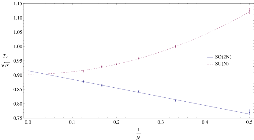
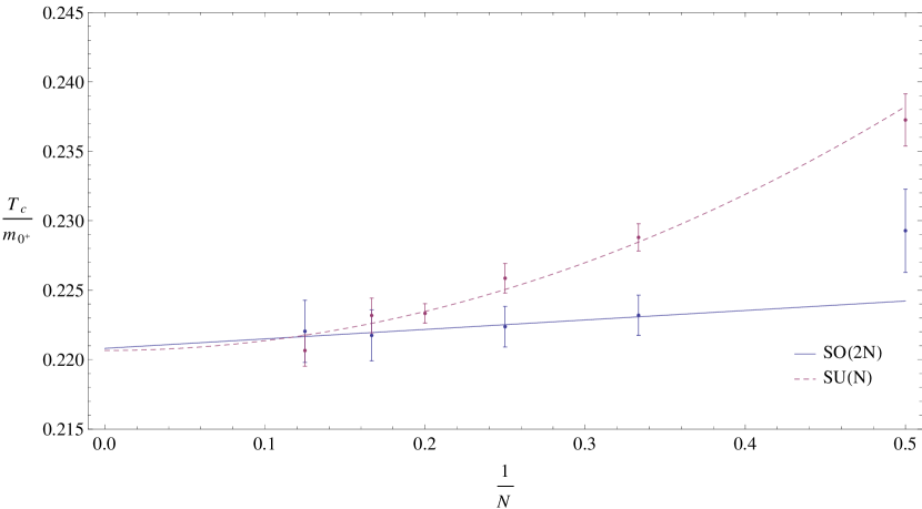
We list the $SO(2N)$ and $SU(N)$ Jack-Liddle:2008xr continuum values of $T_{c}/\surd\sigma$ in Table 29. We display the corresponding large-$N$ extrapolations in Figure 19. The two large-$N$ limits are

$$\frac{T_{c}}{\surd\sigma}=\begin{cases}0.9152(48)\quad SO(2N\rightarrow\infty)&\\ 0.9030(29)\quad SU(N\rightarrow\infty)&\end{cases}.$$ (62)

We see that these two values are within $2\sigma$ of each other, which is consistent with the hypothesis that they are equal. As for the planar equivalence, we recall that fitting $SO(N\geq 3)$ with a fit that is linear in $1/N$ gives $T_{c}/\surd\sigma=0.9194(33)$ at $N=\infty$, and this is a less comfortable $\sim 4\sigma$ from the $SU(\infty)$ value.

Similarly, we list the $SO(2N)$ and $SU(N)$ Liddle:2006aa continuum values of $T_{c}/(g^{2}N)$ in Table 29. To compare the $SO(2N)$ and $SU(N)$ values, we need to rescale the $SO(N)$ values to $SO(2N)$ values by doubling them (as we did in some earlier figures). This is due to the large-$N$ coupling matching $g^{2}_{SU(N)}N=g^{2}_{SO(2N)}N$, so that the large-$N$ limit is

$$\lim_{N\to\infty}\frac{T_{c}}{g^{2}_{SU(N)}N}=\lim_{N\to\infty}\frac{T_{c}}{g^{2}_{SO(2N)}N}=\lim_{N\to\infty}2\frac{T_{c}}{g^{2}_{SO(2N)}2N}.$$ (63)

The two large-$N$ limits are

$$\frac{T_{c}}{g^{2}N}=\begin{cases}0.1828(10)\quad SO(2N\rightarrow\infty)&\\ 0.1852(8)\quad SU(N\rightarrow\infty)&\end{cases}$$ (64)

while a fit to $SO(N\geq 3)$ gives ${T_{c}}/{g^{2}N}=0.1832(7)$. We see that these two values are no more than $\sim 2\sigma$ from each other.

Finally, we list the $SO(2N)$ and $SU(N)$ Jack-Liddle:2008xr ; Lucini:2002oz ; Athenodorou:aa values of $T_{c}/M_{0^{+}}$ Table 29. We display the two large-$N$ extrapolations in Figure 20. The two large-$N$ limits obtained from these leading order fits are

$$\frac{T_{c}}{M_{0^{+}}}=\begin{cases}0.2209(28)\quad&SO(2N\rightarrow\infty)\\ 0.2207(6)\quad&SU(N\rightarrow\infty)\end{cases}.$$ (65)

and a higher order fit to all $SO(N\geq 3)$ gives a value $0.2230(39)$. We see that all these values agree very well.

10 Conclusions

In this paper we identified a finite temperature transition in $D=2+1$ $SO(N)$ gauge theories for $N=4,5,6,7,8,9,12,16$. For $N=4,5$ the transition appears to be second order, while for $N\geq 6$ it appears to be first order. We did not attempt to calculate $T_{c}$ for $SO(3)$ because the inconvenient location of the ‘bulk’ transition would have made it computationally expensive. However, the close connection between $SO(3)$ and $SU(2)$ makes one confident that there is a deconfining transition in $SO(3)$, and we have used the $SU(2)$ value of $T_{c}$ to provide an estimate for the $SO(3)$ value.

This transition appears to have all the characteristics of a deconfining transition for both even and odd $N$, and appears to be a phase transition rather than a cross-over. We gave some arguments, and provided some evidence, that $SO(N)$ gauge theories are indeed confining at low $T$, and that this is the case not just for even $N$ but also for odd $N$ where the centre is trivial.

Our calculations were performed on a lattice in a finite volume, but our final results for the deconfining temperature, $T_{c}$, are for the continuum theory in an infinite volume. (Achieved through extrapolation, of course.) We find that dimensionless ratios such as $T_{c}/\surd\sigma$, where $\sigma$ is the zero-temperature confining string tension, fall on a single sequence that can be interpolated by a smooth function of $N$ for $N\geq 3$ (with the value for $SO(3)$ being inferred from the value in $SU(2)$). That is to say, we can think of the $N$-dependence of non-Abelian $SO(N)$ gauge theories as a continuous function of $N$ for all $N$. In particular there is no evidence that even and odd $N$ fall on two separate (even if converging) branches.

Somewhat remarkably we find that a simple leading-order large-$N$ expression suffices to fit all our calculated values of $T_{c}/\surd\sigma$:

$$\frac{T_{c}}{\surd\sigma}=0.9194(33)-\frac{0.620(28)}{N}\quad;\quad N\geq 3.$$ (66)

Such a ‘precocious’ large-$N$ scaling seems the norm for physical mass ratios in both $SO(N)$ Lau:aa ; Bursa:2013lq and $SU(N)$ Teper:1998rw ; Lucini:2002oz ; Athenodorou:aa gauge theories. Even more striking is how weakly the ratio ${T_{c}}/{M_{0^{+}}}$ depends on $N$, as we see in Figure 20 and as highlighted by the smallness of the leading correction in our higher order fit

$$\frac{T_{c}}{M_{0^{+}}}=0.2230(39)-\frac{0.033(45)}{N}+\frac{0.23(12)}{N^{2}}\quad;\quad N\geq 3.$$ (67)

A possible explanation for this weak $N$-dependence is discussed in Athenodorou:2015aa .

As an aside, we remark that our results, as described in Section 8.2, provide a non-perturbative confirmation of the expected large-$N$ scaling: $g^{2}N$ fixed, and $O(1/N)$ leading corrections as $N\to\infty$.

As another (much less expected) aside, we recall that our values of ${T_{c}}/{\surd\sigma}$ on the strong coupling side of the ‘bulk’ transition also appeared to extrapolate to $a=0$ with a simple $O(a^{2})$ correction. At small $N$ this ‘strong coupling continuum limit’ was very different from the true weak coupling continuum limit, but at larger $N$ they became consistent. This unexpected and bizarre behaviour strongly suggests that our interpretation of the ‘bulk’ transition as a simple strong-to-weak coupling transition is too naive.

Since $SU(N)$ gauge theories can be orbifold projected from $SO(2N)$, we expect them to have the same physics at large $N$ Unsal:2006kx , and indeed we find that the values of $T_{c}$ extrapolated to $N=\infty$ are consistent with being equal, at the $\sim 1\%$ level. We obtain a similar confirmation of the large-$N$ planar equivalence between $SO(N)$ and $SU(N)$ gauge theories. In addition we find that the values of $T_{c}$ in $SO(4)$ and $SO(6)$ are consistent with those in $SU(2)\times SU(2)$ and $SU(4)$ respectively, indicating that for this physics at least the differences in group global structure are not important: theories with the same Lie algebra appear to possess the same value of $T_{c}$.

Appendix A Tables

Data Fit	$\beta_{c}$	$\chi(\beta_{c})$	$\bar{\chi}^{2}_{\text{dof}}$
Reweighting	8.493(10)	25.40(30)	n/a
Gaussian	8.500(11)	25.66(40)	0.62
Logistic	8.500(6)	25.71(41)	0.64

Table 1: Comparisons between reweighting, Gaussian fits, and logistic fits to obtain $\beta_{c}$ and $\chi(\beta_{c})$ on a $40^{2}4$ volume in $SO(4)$.

$L_{s}^{2}L_{t}$	$\beta_{c}$	$\chi_{\left|\overline{l_{P}}\right|}$
$20^{2}2$	6.4748(4)	10.77(4)
$24^{2}2$	6.4771(4)	13.64(5)
$28^{2}2$	6.4788(3)	16.80(9)
$32^{2}2$	6.4797(3)	20.16(8)
$36^{2}2$	6.4813(4)	23.65(12)
$40^{2}2$	6.4819(3)	27.58(14)
$48^{2}2$	6.4822(4)	35.15(43)
$56^{2}2$	6.4840(4)	44.42(63)
$60^{2}2$	6.4850(4)	49.92(89)
$80^{2}2$	6.4853(4)	78.57(132)

$L_{s}^{2}L_{t}$	$\beta_{c}$	$\chi_{\left|\overline{l_{P}}\right|}$
$32^{2}3$	7.534(3)	19.60(14)
$36^{2}3$	7.538(3)	23.22(16)
$40^{2}3$	7.539(1)	26.37(25)
$44^{2}3$	7.545(2)	31.09(38)
$48^{2}3$	7.546(3)	35.56(38)
$52^{2}3$	7.552(2)	40.58(53)
$66^{2}3$	7.552(2)	58.75(131)
$80^{2}3$	7.555(3)	81.02(193)
$90^{2}3$	7.557(3)	95.80(171)
$40^{2}4$	8.493(10)	25.40(30)
$48^{2}4$	8.501(6)	33.88(56)
$56^{2}4$	8.509(8)	42.02(93)
$64^{2}4$	8.526(7)	51.67(120)
$72^{2}4$	8.520(3)	59.46(140)
$80^{2}4$	8.535(6)	66.44(173)
$88^{2}4$	8.545(8)	75.23(296)

Table 2: $\beta_{c}$ and $\chi_{\left|\overline{l_{P}}\right|}$ in $SO(4)$ for $L_{t}\leq 4$ on various volumes.

$L_{s}^{2}L_{t}$	$\beta_{c}$	$\chi_{\left|\overline{l_{P}}\right|}$
$36^{2}6$	11.110(31)	20.68(18)
$48^{2}6$	10.924(17)	28.87(36)
$60^{2}6$	10.861(9)	38.76(53)
$72^{2}6$	10.837(14)	47.33(83)
$84^{2}6$	10.809(21)	57.82(125)
$96^{2}6$	10.824(14)	70.28(199)
$120^{2}6$	10.835(8)	95.57(321)
$42^{2}7$	12.685(45)	29.41(38)
$56^{2}7$	12.494(22)	41.46(64)
$70^{2}7$	12.397(12)	54.24(94)
$84^{2}7$	12.303(12)	68.11(111)
$98^{2}7$	12.224(12)	81.74(172)
$112^{2}7$	12.261(19)	100.03(247)
$126^{2}7$	12.274(19)	117.10(302)

$L_{s}^{2}L_{t}$	$\beta_{c}$	$\chi_{\left|\overline{l_{P}}\right|}$
$64^{2}8$	14.005(37)	55.93(88)
$80^{2}8$	13.836(24)	71.23(136)
$96^{2}8$	13.901(16)	93.98(248)
$112^{2}8$	13.712(16)	106.33(214)
$128^{2}8$	13.736(14)	131.84(390)
$144^{2}8$	13.767(20)	158.18(629)
$80^{2}10$	17.096(31)	95.93(174)
$90^{2}10$	16.919(35)	107.06(234)
$100^{2}10$	16.870(24)	127.64(305)
$110^{2}10$	16.790(53)	137.15(367)
$120^{2}10$	16.731(24)	154.83(462)
$140^{2}10$	16.725(23)	184.45(659)
$72^{2}12$	20.648(62)	107.12(158)
$84^{2}12$	20.202(66)	122.92(199)
$96^{2}12$	20.098(52)	144.13(252)
$120^{2}12$	19.797(29)	190.28(414)
$144^{2}12$	19.757(27)	236.11(603)

Table 3: $\beta_{c}$ and $\chi_{\left|\overline{l_{P}}\right|}$ in $SO(4)$ for $L_{t}\geq 6$ on various volumes.

$L_{t}$	$\beta_{c}(V\rightarrow\infty)$	$L_{s}$ range	$\bar{\chi}^{2}_{\text{dof}}$
2	6.4891(3)	$L_{s}\geq 20$	1.19
3	7.573(3)	$L_{s}\geq 32$	1.44
4	8.573(10)	$L_{s}\geq 40$	1.24
6	10.781(16)	$L_{s}\geq 48$	2.77
7	11.980(24)	$L_{s}\geq 42$	6.49
8	13.504(34)	$L_{s}\geq 64$	13.18
10	16.321(80)	$L_{s}\geq 90$	1.19
12	19.090(99)	$L_{s}\geq 84$	3.13

Table 4: Infinite volume limit of $\beta_{c}$, range of volumes used and $\bar{\chi}^{2}_{\text{dof}}$ of extrapolation, for $SO(4)$.

$L_{s}^{2}L_{t}$	$\beta_{c}$	$\chi_{\left|\overline{l_{P}}\right|}$
$16^{2}2$	10.380(1)	10.75(3)
$18^{2}2$	10.378(1)	12.82(4)
$20^{2}2$	10.378(1)	14.74(7)
$22^{2}2$	10.376(1)	16.83(9)
$24^{2}2$	10.377(2)	18.53(12)
$26^{2}3$	12.058(3)	13.41(14)
$28^{2}3$	12.054(3)	14.07(15)
$30^{2}3$	12.049(3)	14.76(12)
$32^{2}3$	12.053(4)	15.28(15)
$34^{2}3$	12.049(4)	16.02(25)
$32^{2}4$	13.964(10)	16.42(12)
$36^{2}4$	13.964(9)	18.90(13)
$40^{2}4$	13.955(7)	21.27(18)
$48^{2}4$	13.962(12)	24.13(27)
$40^{2}5$	16.316(14)	20.75(14)
$44^{2}5$	16.342(8)	24.15(23)
$50^{2}5$	16.300(13)	26.37(20)
$54^{2}5$	16.295(26)	27.87(18)
$60^{2}5$	16.265(8)	30.58(29)
$70^{2}5$	16.290(6)	35.40(40)

$L_{s}^{2}L_{t}$	$\beta_{c}$	$\chi_{\left|\overline{l_{P}}\right|}$
$42^{2}6$	19.017(34)	28.35(49)
$48^{2}6$	18.939(61)	31.74(41)
$54^{2}6$	18.965(19)	36.39(49)
$60^{2}6$	18.930(18)	40.39(76)
$56^{2}7$	21.715(17)	46.57(67)
$60^{2}7$	21.663(16)	48.70(77)
$64^{2}7$	21.592(15)	53.02(81)
$68^{2}7$	21.595(15)	55.50(90)
$72^{2}7$	21.554(11)	58.01(99)
$84^{2}7$	21.564(17)	69.48(159)
$64^{2}8$	24.329(24)	63.20(102)
$72^{2}8$	24.294(18)	72.14(124)
$80^{2}8$	24.255(14)	80.30(154)
$88^{2}8$	24.255(17)	85.77(180)
$96^{2}8$	24.182(18)	83.53(197)
$80^{2}10$	29.730(19)	109.84(163)
$90^{2}10$	29.621(26)	116.99(200)
$100^{2}10$	29.521(19)	130.84(236)
$110^{2}10$	29.519(19)	141.11(272)
$120^{2}10$	29.517(22)	159.53(391)

Table 5: $\beta_{c}(V)$ and $\chi_{\left|\overline{l_{P}}\right|}(V)$ for $SO(5)$.

$L_{t}$	$\beta_{c}(V\rightarrow\infty)$	$L_{s}$ range	$\bar{\chi}^{2}_{\text{dof}}$
2	10.368(3)	$L_{s}\geq 16$	0.74
3	12.021(16)	$L_{s}\geq 26$	0.49
4	13.944(36)	$L_{s}\geq 32$	0.32
5	16.180(13)	$L_{s}\geq 40$	4.56
6	18.603(55)	$L_{s}\geq 42$	1.29
7	21.192(52)	$L_{s}\geq 56$	4.63
8	23.938(63)	$L_{s}\geq 64$	1.39
10	29.500(157)	$L_{s}\geq 100$	0.00

Table 6: Infinite volume limit of $\beta_{c}$, range of volumes used and $\bar{\chi}^{2}_{\text{dof}}$ of extrapolation, for $SO(5)$.

$L_{s}^{2}L_{t}$	$\beta_{c}$	$\chi_{\left|\overline{l_{P}}\right|}$
$8^{2}2$	15.175(2)	3.191(8)
$10^{2}2$	15.185(1)	4.972(8)
$12^{2}2$	15.192(1)	7.151(12)
$12^{2}3$	17.810(9)	3.94(1)
$16^{2}3$	17.793(4)	6.22(2)
$20^{2}3$	17.821(4)	9.18(3)
$24^{2}3$	17.831(4)	12.34(5)
$28^{2}3$	17.833(3)	15.79(8)
$32^{2}3$	17.839(3)	19.53(13)
$28^{2}4$	21.295(6)	12.07(5)
$32^{2}4$	21.358(8)	15.56(12)
$36^{2}4$	21.356(8)	18.58(9)
$40^{2}4$	21.352(4)	22.23(13)
$44^{2}4$	21.370(6)	25.85(15)

$L_{s}^{2}L_{t}$	$\beta_{c}$	$\chi_{\left|\overline{l_{P}}\right|}$
$28^{2}5$	25.479(24)	14.25(8)
$32^{2}5$	25.496(16)	17.77(12)
$40^{2}5$	25.501(14)	25.25(18)
$48^{2}5$	25.549(14)	33.99(38)
$56^{2}5$	25.577(11)	44.40(41)
$60^{2}5$	25.589(10)	48.77(68)
$42^{2}6$	29.781(26)	31.45(18)
$48^{2}6$	29.727(18)	38.65(30)
$54^{2}6$	29.791(33)	47.09(75)
$60^{2}6$	29.796(31)	55.66(75)
$66^{2}6$	29.819(9)	65.52(89)
$44^{2}7$	34.031(37)	38.73(30)
$50^{2}7$	33.907(25)	46.75(48)
$56^{2}7$	34.078(49)	57.24(96)
$60^{2}7$	34.042(36)	62.06(65)
$64^{2}7$	34.021(19)	69.71(85)
$68^{2}7$	34.009(25)	75.83(107)
$72^{2}7$	34.092(23)	83.87(143)

Table 7: $\beta_{c}(V)$ and $\chi_{\left|\overline{l_{P}}\right|}(V)$ for $SO(6)$.

$L_{t}$	$\beta_{c}(V\rightarrow\infty)$	$L_{s}$ range	$\bar{\chi}^{2}_{\text{dof}}$
2	15.205(3)	$L_{s}\geq 8$	0.62
3	17.854(3)	$L_{s}\geq 12$	0.83
4	21.399(6)	$L_{s}\geq 28$	6.42
5	25.613(11)	$L_{s}\geq 28$	2.25
6	29.872(21)	$L_{s}\geq 42$	2.79
7	34.113(32)	$L_{s}\geq 44$	4.44

Table 8: Infinite volume limit of $\beta_{c}$, range of volumes used and $\bar{\chi}^{2}_{\text{dof}}$ of extrapolation, for $SO(6)$.

$L_{s}^{2}L_{t}$	$\beta_{c}$	$\chi_{\left|\overline{l_{P}}\right|}$
$8^{2}2$	20.963(3)	3.347(3)
$10^{2}2$	20.960(3)	5.381(10)
$12^{2}2$	20.953(3)	7.916(14)
$12^{2}3$	25.148(29)	4.00(3)
$16^{2}3$	25.022(14)	6.60(4)
$20^{2}3$	24.982(13)	9.96(8)
$24^{2}3$	24.988(5)	14.27(7)
$28^{2}3$	25.011(7)	19.40(14)
$24^{2}4$	30.721(24)	12.65(12)
$32^{2}4$	30.714(21)	21.04(30)
$40^{2}4$	30.721(7)	31.62(27)
$48^{2}4$	30.727(6)	44.05(43)
$56^{2}4$	30.726(8)	58.67(67)

$L_{s}^{2}L_{t}$	$\beta_{c}$	$\chi_{\left|\overline{l_{P}}\right|}$
$32^{2}5$	36.909(20)	23.75(21)
$40^{2}5$	36.885(19)	35.40(43)
$48^{2}5$	36.895(24)	50.05(80)
$56^{2}5$	36.930(22)	66.59(110)
$64^{2}5$	36.909(19)	83.37(151)
$52^{2}6$	43.088(25)	62.57(104)
$56^{2}6$	43.089(10)	72.92(93)
$60^{2}6$	43.164(14)	83.65(127)
$64^{2}6$	43.129(17)	94.02(115)

Table 9: $\beta_{c}(V)$ and $\chi_{\left|\overline{l_{P}}\right|}(V)$ for $SO(7)$.

$L_{t}$	$\beta_{c}(V\rightarrow\infty)$	$L_{s}$ range	$\bar{\chi}^{2}_{\text{dof}}$
2	20.947(6)	$L_{s}\geq 8$	0.82
3	24.992(11)	$L_{s}\geq 12$	5.46
4	30.729(9)	$L_{s}\geq 24$	0.14
5	36.913(20)	$L_{s}\geq 32$	0.81
6	43.311(62)	$L_{s}\geq 52$	5.00

Table 10: Infinite volume limit of $\beta_{c}$, range of volumes used and $\bar{\chi}^{2}_{\text{dof}}$ of extrapolation, for $SO(7)$.

$L_{s}^{2}L_{t}$	$\beta_{c}$	$\chi_{\left|\overline{l_{P}}\right|}$
$8^{2}2$	27.583(4)	3.241(4)
$10^{2}2$	27.594(3)	5.279(6)
$12^{2}2$	27.605(3)	7.851(7)
$16^{2}3$	33.488(22)	6.29(6)
$18^{2}3$	33.503(17)	8.05(7)
$20^{2}3$	33.468(13)	9.68(5)
$24^{2}3$	33.521(8)	14.54(7)
$24^{2}4$	41.573(14)	13.20(6)
$28^{2}4$	41.600(18)	17.88(16)
$32^{2}4$	41.631(14)	23.71(17)
$40^{2}4$	41.686(14)	37.98(28)

$L_{s}^{2}L_{t}$	$\beta_{c}$	$\chi_{\left|\overline{l_{P}}\right|}$
$32^{2}5$	50.073(23)	25.70(27)
$40^{2}5$	50.163(21)	40.21(40)
$48^{2}5$	50.178(37)	58.72(72)
$56^{2}5$	50.247(22)	81.93(90)
$42^{2}6$	58.560(18)	46.27(34)
$48^{2}6$	58.742(24)	63.38(78)
$54^{2}6$	58.703(19)	79.59(60)
$60^{2}6$	58.758(12)	101.15(99)

Table 11: $\beta_{c}(V)$ and $\chi_{\left|\overline{l_{P}}\right|}(V)$ for $SO(8)$.

$L_{t}$	$\beta_{c}(V\rightarrow\infty)$	$L_{s}$ range	$\bar{\chi}^{2}_{\text{dof}}$
2	27.622(5)	$L_{s}\geq 8$	0.66
3	33.547(21)	$L_{s}\geq 16$	4.06
4	41.769(32)	$L_{s}\geq 24$	0.22
5	50.319(32)	$L_{s}\geq 32$	0.46
6	58.935(29)	$L_{s}\geq 42$	6.65

Table 12: Infinite volume limit of $\beta_{c}$, range of volumes used and $\bar{\chi}^{2}_{\text{dof}}$ of extrapolation, for $SO(8)$.

$L_{s}^{2}L_{t}$	$\beta_{c}$	$\chi_{\left|\overline{l_{P}}\right|}$
$16^{2}3$	43.443(9)	6.79(2)
$18^{2}3$	43.425(6)	8.64(2)
$20^{2}3$	43.427(7)	10.80(4)
$22^{2}3$	43.431(7)	13.26(5)
$24^{2}3$	43.460(7)	16.16(5)
$26^{2}3$	43.457(6)	19.17(6)
$30^{2}3$	43.424(7)	25.59(9)
$36^{2}3$	43.433(12)	37.59(26)
$42^{2}3$	43.399(8)	51.23(30)

$L_{s}^{2}L_{t}$	$\beta_{c}$	$\chi_{\left|\overline{l_{P}}\right|}$
$20^{2}4$	54.449(28)	10.96(10)
$24^{2}4$	54.375(28)	15.93(14)
$28^{2}4$	54.393(19)	22.01(16)
$32^{2}4$	54.505(17)	30.22(18)
$40^{2}4$	54.464(14)	48.16(26)
$48^{2}4$	54.434(12)	70.28(55)
$24^{2}5$	65.634(38)	16.87(9)
$28^{2}5$	65.654(46)	23.34(16)
$32^{2}5$	65.661(38)	31.17(22)
$36^{2}5$	65.674(15)	40.16(22)
$40^{2}5$	65.648(20)	50.10(36)
$48^{2}5$	65.760(17)	75.33(53)

Table 13: $\beta_{c}(V)$ and $\chi_{\left|\overline{l_{P}}\right|}(V)$ for $SO(9)$.

$L_{t}$	$\beta_{c}(V\rightarrow\infty)$	$L_{s}$ range	$\bar{\chi}^{2}_{\text{dof}}$
3	43.450(7)	$L_{s}\geq 16$	6.10
4	54.457(13)	$L_{s}\geq 20$	6.78
5	65.678(32)	$L_{s}\geq 24$	0.47

Table 14: Infinite volume limit of $\beta_{c}$, range of volumes used and $\bar{\chi}^{2}_{\text{dof}}$ of extrapolation, for $SO(9)$.

$L_{s}^{2}L_{t}$	$\beta_{c}$	$\chi_{\left|\overline{l_{P}}\right|}$
$6^{2}2$	63.57(1)	1.593(1)
$7^{2}2$	63.59(1)	2.248(1)
$8^{2}2$	63.58(1)	3.014(3)
$8^{2}3$	80.72(1)	1.620(3)
$10^{2}3$	80.83(1)	2.640(8)
$12^{2}3$	80.96(1)	4.043(8)
$14^{2}3$	81.05(1)	5.800(16)
$16^{2}3$	81.12(1)	7.929(17)

$L_{s}^{2}L_{t}$	$\beta_{c}$	$\chi_{\left|\overline{l_{P}}\right|}$
$12^{2}4$	101.81(5)	3.995(25)
$16^{2}4$	102.11(8)	7.619(84)
$20^{2}4$	102.19(4)	12.739(71)
$24^{2}4$	102.28(4)	19.393(88)
$16^{2}5$	123.03(10)	7.709(60)
$20^{2}5$	123.26(8)	12.988(104)
$24^{2}5$	123.52(4)	19.769(137)
$28^{2}5$	123.62(6)	27.835(284)

Table 15: $\beta_{c}(V)$ and $\chi_{\left|\overline{l_{P}}\right|}(V)$ for $SO(12)$.

$L_{t}$	$\beta_{c}(V\rightarrow\infty)$	$L_{s}$ range	$\bar{\chi}^{2}_{\text{dof}}$
2	63.610(14)	$L_{s}\geq 6$	3.35
3	81.299(17)	$L_{s}\geq 8$	0.70
4	102.424(45)	$L_{s}\geq 12$	0.16
5	124.011(15)	$L_{s}\geq 16$	0.34

Table 16: Infinite volume limit of $\beta_{c}$, range of volumes used and $\bar{\chi}^{2}_{\text{dof}}$ of extrapolation, for $SO(12)$.

$L_{s}^{2}L_{t}$	$\beta_{c}$	$\chi_{\left|\overline{l_{P}}\right|}$
$4^{2}2$	114.85(2)	0.595(1)
$5^{2}2$	114.82(2)	0.998(2)
$6^{2}2$	114.84(2)	1.512(3)
$6^{2}3$	149.17(2)	0.940(2)
$8^{2}3$	149.32(2)	1.832(3)
$10^{2}3$	149.58(3)	3.141(4)
$12^{2}3$	149.76(2)	4.839(10)
$14^{2}3$	149.89(3)	6.897(20)

$L_{s}^{2}L_{t}$	$\beta_{c}$	$\chi_{\left|\overline{l_{P}}\right|}$
$6^{2}4$	192.07(26)	1.016(7)
$8^{2}4$	189.04(32)	1.804(25)
$10^{2}4$	188.91(17)	3.011(42)
$12^{2}4$	189.13(11)	4.617(47)
$14^{2}4$	189.33(11)	6.725(74)
$16^{2}4$	189.55(6)	9.221(40)
$8^{2}5$	230.62(44)	1.972(18)
$10^{2}5$	229.42(56)	3.013(44)
$12^{2}5$	228.60(5)	4.591(14)
$14^{2}5$	228.77(6)	6.572(18)
$16^{2}5$	229.01(7)	9.036(31)
$20^{2}5$	229.51(12)	15.429(88)

Table 17: $\beta_{c}(V)$ and $\chi_{\left|\overline{l_{P}}\right|}(V)$ for $SO(16)$.

$L_{t}$	$\beta_{c}(V\rightarrow\infty)$	$L_{s}$ range	$\bar{\chi}^{2}_{\text{dof}}$
2	114.824(35)	$L_{s}\geq 4$	0.66
3	150.128(33)	$L_{s}\geq 8$	0.83
4	189.975(14)	$L_{s}\geq 12$	0.19
5	230.096(212)	$L_{s}\geq 14$	1.06

Table 18: Infinite volume limit of $\beta_{c}$, range of volumes used and $\bar{\chi}^{2}_{\text{dof}}$ of extrapolation, for $SO(16)$.

$N$	$L_{s}^{2}L_{t}$	Bulk transition	Weak coupling region
$4$	$20^{2}24$	$\beta\in[9.1,10.2]$	$L_{t}\geq 6$
$5$	$12^{2}24$	$\beta\in[13.5,15.4]$	$L_{t}\geq 5$
$6$	$12^{2}24$	$\beta\in[18.0,21.3]$	$L_{t}\geq 5$
$7$	$8^{2}24$	$\beta\in[23.5,28.0]$	$L_{t}\geq 4$
$8$	$8^{2}24$	$\beta\in[31,35]$	$L_{t}\geq 4$
$9$	$4^{2}24$	$\beta\in[37,42]$	$L_{t}\geq 3$
$12$	$4^{2}24$	$\beta\in[65,73]$	$L_{t}\geq 3$
$16$	$2^{2}24$	$\beta\in[111,124]$	$L_{t}\geq 3$

Table 19: Location of the bulk transition on volumes $L_{s}^{2}L_{t}$, and consequent range of $L_{t}$ for which $\beta_{c}$ is on weak coupling side.

$L_{t}$	$\beta_{c}(V\rightarrow\infty)$	$a\surd\sigma$	$T_{c}/\surd\sigma$	$\beta_{I}(V\rightarrow\infty)$	$T_{c}/(g^{2}N)$	Coupling
2	6.4891(3)	0.6208(3)	0.8054(3)	3.7234(5)	0.05818(1)	Strong
3	7.573(3)	0.3970(7)	0.8397(14)	5.169(3)	0.05384(3)
4	8.573(10)	0.2936(10)	0.8515(31)	6.290(11)	0.04914(8)
6	10.781(16)	0.2146(17)	0.7766(60)	8.590(16)	0.04474(8)	Weak
7	11.980(24)	0.1845(11)	0.7743(44)	9.816(24)	0.04382(11)
8	13.504(34)	0.1609(12)	0.7770(60)	11.364(34)	0.04439(13)
10	16.322(80)	0.1206(13)	0.7718(81)	14.213(81)	0.04442(25)
12	19.090(99)	0.1083(15)	0.7692(106)	17.099(76)	0.04453(20)

Table 20: $SO(4)$ critical temperature in units of the string tension, $T_{c}/\surd\sigma$, and in units of the (mean field improved) ’t Hooft coupling, $T_{c}/(g^{2}N)$, evaluated at $\beta_{c}(V\rightarrow\infty)$.

$L_{t}$	$\beta_{c}(V\rightarrow\infty)$	$a\surd\sigma$	$T_{c}/\surd\sigma$	$\beta_{I}(V\rightarrow\infty)$	$T_{c}/(g^{2}N)$	Coupling
2	10.368(3)	0.6447(14)	0.7756(17)	5.811(5)	0.05811(5)	Strong
3	12.021(16)	0.4248(19)	0.7847(36)	8.044(19)	0.05363(13)
4	13.944(36)	0.3214(15)	0.7778(36)	10.162(39)	0.05081(19)
5	16.180(13)	0.2593(15)	0.7714(44)	12.497(13)	0.04999(5)	Weak
6	18.603(55)	0.2190(12)	0.7611(43)	14.985(56)	0.04995(19)
7	21.192(52)	0.1877(11)	0.7613(45)	17.620(53)	0.05034(15)
8	23.938(63)	0.1624(9)	0.7698(41)	10.401(64)	0.05100(16)
10	29.500(157)	0.1281(10)	0.7801(62)	26.010(158)	0.05202(32)

Table 21: $SO(5)$ critical temperature in units of the string tension, $T_{c}/\surd\sigma$, and in units of the (mean field improved) ’t Hooft coupling, $T_{c}/(g^{2}N)$, evaluated at $\beta_{c}(V\rightarrow\infty)$.

$L_{t}$	$\beta_{c}(V\rightarrow\infty)$	$a\surd\sigma$	$T_{c}/\surd\sigma$	$\beta_{I}(V\rightarrow\infty)$	$T_{c}/(g^{2}N)$	Coupling
2	15.205(3)	0.6535(13)	0.7651(15)	8.460(4)	0.05875(3)	Strong
3	17.854(3)	0.4201(7)	0.7935(13)	11.964(4)	0.05539(2)
4	21.399(6)	0.3106(10)	0.8050(27)	15.784(6)	0.05480(2)
5	25.613(11)	0.2501(7)	0.7996(22)	20.147(11)	0.05596(3)	Weak
6	29.872(21)	0.2077(3)	0.8024(14)	24.497(21)	0.05670(5)
7	34.113(32)	0.1774(4)	0.8053(19)	28.798(32)	0.05714(6)

Table 22: $SO(6)$ critical temperature in units of the string tension, $T_{c}/\surd\sigma$, and in units of the (mean field improved) ’t Hooft coupling, $T_{c}/(g^{2}N)$, evaluated at $\beta_{c}(V\rightarrow\infty)$.

$L_{t}$	$\beta_{c}(V\rightarrow\infty)$	$a\surd\sigma$	$T_{c}/\surd\sigma$	$\beta_{I}(V\rightarrow\infty)$	$T_{c}/(g^{2}N)$	Coupling
2	20.947(6)	0.6571(8)	0.7610(10)	11.597(9)	0.05917(4)	Strong
3	24.992(11)	0.4181(7)	0.7972(13)	16.816(12)	0.05720(4)
4	30.729(9)	0.3104(5)	0.8053(12)	22.924(10)	0.05848(2)	Weak
5	36.913(20)	0.2455(7)	0.8147(22)	29.302(20)	0.05980(4)
6	43.311(62)	0.2023(6)	0.8239(26)	35.821(63)	0.06092(11)

Table 23: $SO(7)$ critical temperature in units of the string tension, $T_{c}/\surd\sigma$, and in units of the (mean field improved) ’t Hooft coupling, $T_{c}/(g^{2}N)$, evaluated at $\beta_{c}(V\rightarrow\infty)$.

$L_{t}$	$\beta_{c}(V\rightarrow\infty)$	$a\surd\sigma$	$T_{c}/\surd\sigma$	$\beta_{I}(V\rightarrow\infty)$	$T_{c}/(g^{2}N)$	Coupling
2	27.622(5)	0.6586(8)	0.7591(9)	15.266(8)	0.05963(3)	Strong
3	33.547(21)	0.4179(7)	0.7977(14)	22.715(23)	0.05915(6)
4	41.769(32)	0.3051(11)	0.8193(28)	31.414(33)	0.06136(6)	Weak
5	50.319(32)	0.2415(4)	0.8281(15)	40.210(32)	0.06283(5)
6	58.935(29)	0.2003(5)	0.8320(20)	48.975(29)	0.06377(4)

Table 24: $SO(8)$ critical temperature in units of the string tension, $T_{c}/\surd\sigma$, and in units of the (mean field improved) ’t Hooft coupling, $T_{c}/(g^{2}N)$, evaluated at $\beta_{c}(V\rightarrow\infty)$.

$L_{t}$	$\beta_{c}(V\rightarrow\infty)$	$a\surd\sigma$	$T_{c}/\surd\sigma$	$\beta_{I}(V\rightarrow\infty)$	$T_{c}/(g^{2}N)$	Coupling
3	43.450(7)	0.4150(2)	0.8032(4)	29.586(8)	0.060877(16)	Weak
4	54.457(13)	0.3025(4)	0.8263(11)	41.190(13)	0.063564(21)
5	65.678(32)	0.2395(3)	0.8351(12)	52.714(33)	0.065079(40)

Table 25: $SO(9)$ critical temperature in units of the string tension, $T_{c}/\surd\sigma$, and in units of the (mean field improved) ’t Hooft coupling, $T_{c}/(g^{2}N)$, evaluated at $\beta_{c}(V\rightarrow\infty)$.

$L_{t}$	$\beta_{c}(V\rightarrow\infty)$	$a\surd\sigma$	$T_{c}/\surd\sigma$	$\beta_{I}(V\rightarrow\infty)$	$T_{c}/(g^{2}N)$	Coupling
2	63.610(14)	0.6600(24)	0.7576(27)	35.213(22)	0.06113(4)	Strong
3	81.299(17)	0.4070(6)	0.8191(12)	56.114(18)	0.064947(21)	Weak
4	102.424(45)	0.2977(6)	0.8399(18)	78.245(46)	0.06792(4)
5	124.011(15)	0.2354(12)	0.8497(43)	100.359(180)	0.06969(12)

Table 26: $SO(12)$ critical temperature in units of the string tension, $T_{c}/\surd\sigma$, and in units of the (mean field improved) ’t Hooft coupling, $T_{c}/(g^{2}N)$, evaluated at $\beta_{c}(V\rightarrow\infty)$.

$L_{t}$	$\beta_{c}(V\rightarrow\infty)$	$a\surd\sigma$	$T_{c}/\surd\sigma$	$\beta_{I}(V\rightarrow\infty)$	$T_{c}/(g^{2}N)$	Coupling
2	63.610(14)	0.6438(25)	0.7766(31)	64.219(47)	0.06271(5)	Strong
3	81.299(17)	0.4003(12)	0.8328(24)	104.617(35)	0.068110(23)	Weak
4	102.424(45)	0.2925(9)	0.8547(26)	146.288(207)	0.07143(10)
5	124.011(15)	0.2320(7)	0.8622(28)	187.090(218)	0.07308(9)

Table 27: $SO(16)$ critical temperature in units of the string tension, $T_{c}/\surd\sigma$, and in units of the (mean field improved) ’t Hooft coupling, $T_{c}/(g^{2}N)$, evaluated at $\beta_{c}(V\rightarrow\infty)$.

$N$	$T_{c}/\surd\sigma$	$\bar{\chi}^{2}_{\text{dof}}$	$T_{c}/(g^{2}N)$	$\bar{\chi}^{2}_{\text{dof}}$	$T_{c}/M_{0^{+}}$
3*	0.7072(80)		0.03236(45)		0.2373(33)
4	0.7702(88)	0.12	0.04567(43)	2.17	0.2293(30)
5	0.7963(114)	0.00	0.05544(93)	0.05	0.2244(33)
6	0.8105(42)	0.16	0.05996(19)	0.53	0.2232(14)
7	0.8351(38)	0.98	0.06478(18)	4.01	0.2234(12)
8	0.8418(39)	0.05	0.06809(16)	0.00	0.2224(15)
9	0.8515(15)	0.30	0.07043(7)	0.10
12	0.8642(38)	0.02	0.07552(14)	0.63	0.2217(18)
16	0.8780(38)	0.15	0.07947(17)	0.85	0.2220(22)

Table 28: $SO(N)$ continuum limit of the deconfining temperature in units of the string tension, $T_{c}/\surd\sigma$, of the ’t Hooft coupling, $T_{c}/(g^{2}N)$, and of the lightest scalar glueball mass, $T_{c}/M_{0^{+}}$, with corresponding $\bar{\chi}^{2}_{\text{dof}}$ of the fits. Note that we infer the $SO(3)$ value (*) from the $SU(2)$ value.

	$T_{c}/\surd\sigma$		$T_{c}/g^{2}N$		$T_{c}/M_{0^{+}}$
$N$	$SO(2N)$	$SU(N)$	$SO(2N)$	$SU(N)$	$SO(2N)$	$SU(N)$
2	0.7702(88)	1.1238(88)	0.0913(9)	0.1998(34)	0.2293(30)	0.2373(19)
3	0.8105(42)	0.9994(40)	0.1199(4)	0.1904(12)	0.2232(14)	0.2288(10)
4	0.8418(39)	0.9572(39)	0.1362(3)	0.1884(12)	0.2224(15)	0.2259(11)
5		0.9380(19)		0.1874(10)		0.2233(7)
6	0.8642(38)	0.9300(48)	0.1510(3)	0.1873(8)	0.2217(18)	0.2232(12)
8	0.8780(38)	0.9144(41)	0.1589(3)	0.1849(10)	0.2220(22)	0.2207(11)

Table 29: $SO(2N)$ and $SU(N)$ Jack-Liddle:2008xr continuum limit of the deconfining temperature in units of the string tension, $T_{c}/\surd\sigma$, the ’t Hooft coupling, $T_{c}/(g^{2}N)$, and the lightest scalar glueball mass, $T_{c}/M_{0^{+}}$.

Appendix B Figures

Figure 1: Susceptibility plots (renormalised) for the spatial plaquette $\overline{U}_{s}$, the temporal plaquette $\overline{U}_{t}$, and the modulus of the averaged Polyakov loop $\left|\overline{l_{P}}\right|$ for $SO(4)$ on a $32^{2}3$ lattice.

Figure 2: The Polyakov loop $\Braket{\left missing}{\overline{l_{P}}}{}$ for $SO(6)$ on a $20^{2}3$ lattice. The vertical lines, spanning the transition, correspond to $\beta=(\beta_{-},\beta_{0},\beta_{+})=(17.5,17.8,18.1)$.

Figure 3: Average value of Polyakov loop on a $48^{2}4$ lattice in $SO(7)$ versus $\beta$.

Figure 4: Polyakov loop $\overline{l_{P}}$ histograms at $\beta=\beta_{-},\beta_{0},\beta_{+}$ (see Figure 2) for $SO(6)$ on a $20^{2}3$ lattice.

Figure 5: Polyakov loop $\overline{l_{P}}$ history plots at $\beta=\beta_{-},\beta_{0},\beta_{+}$ (see Figure 2) for $SO(6)$ on a $20^{2}3$ lattice from a run of $10^{6}$ configurations.

Figure 6: The value of the averaged Polyakov loop, taken every 25 sweeps, on a $48^{2}4$ lattice in $SO(7)$ versus the number of sweeps $n$.

Figure 7: Probability (unnormalised) of the Polyakov loop averaged over the spatial volume of a $48^{2}4$ lattice in $SO(7)$ for $T\simeq 0.96T_{c}$, $\circ$, $T\simeq T_{c}$, $\bullet$, and $T\simeq 1.04T_{c}$, $\Box$.

Figure 8: Polyakov loop $\overline{l_{P}}$ histograms for $SO(4)$ on a $28^{2}2$ lattice.

Figure 9: Fitting the Polyakov loop susceptibility in $SO(4)$ on a $40^{2}4$ lattice. The points represent our calculations while the continuous black line represents reweighted values. Other lines are curve fits, using the data from the dark points rather than the light points to reduce the $\bar{\chi}^{2}_{\text{dof}}$ of the fits.

Figure 10: The reweighted susceptibility compared to our data, for a $20^{2}3$ lattice in $SO(6)$. The vertical and horizontal lines correspond to the values at the maximum of the susceptibility with its error: $\beta_{c}=17.821(4)$ and $\chi_{\left|\overline{l_{P}}\right|}(\beta_{c})=9.18(3)$

Figure 11: The infinite volume extrapolation for $SO(4)$ with $L_{t}=2$.

Figure 12: The infinite volume extrapolation (using dark points only) for $SO(16)$ with $L_{t}=3$ and with a range of $L_{s}$ values.

Figure 13: Susceptibility volume dependence for $SO(4)$ and $L_{t}=2$.

Figure 14: Susceptibility volume dependence for $SO(8)$ and $L_{t}=5$.

Figure 15: Continuum extrapolation of $SO(4)$ deconfining temperature in units of the string tension.

Figure 16: Continuum extrapolation of $SO(6)$ deconfining temperature in units of the string tension.

Figure 17: Large-$N$ extrapolation of $SO(2N)$ deconfining temperature in units of the string tension. Plotted points include both $SO(2N)$ and $SO(2N+1)$.

Figure 18: Large-$N$ extrapolation of $SO(2N)$ deconfining temperature in units of the lightest scalar glueball mass. Plotted points include both $SO(2N)$ and $SO(2N+1)$.

Figure 19: Large-$N$ extrapolations of $SO(2N)$ and $SU(N)$ deconfining temperatures in units of the string tension.

Figure 20: Large-$N$ extrapolation of $SO(2N)$ and $SU(N)$ deconfining temperatures in units of the lightest scalar glueball mass.

References

- (1) Jack Liddle and Michael Teper. The deconfining phase transition in gauge theories. arXiv:0803.2128, 2008.
- (2) C. Lovelace. Universality at large . Nuclear Physics B, 201(2):333 – 340, 1982.
-
(3)
Shamit Kachru and Eva Silverstein.
4D conformal field theories and strings on orbifolds.
Phys. Rev. Lett., 80:4855–4858, Jun 1998.
Michael Bershadsky and Andrei Johansen. Large limit of orbifold field theories. Nuclear Physics B, 536(1–2):141 – 148, 1998.
Martin Schmaltz. Duality of nonsupersymmetric large gauge theories. Phys. Rev. D, 59:105018, Apr 1999.
M. Strassler. On methods for extracting exact nonperturbative results in nonsupersymmetric gauge theories. arXiv:hep-th/0104032.
Aleksey Cherman, Masanori Hanada, and Daniel Robles-Llana. Orbifold equivalence and the sign problem at finite baryon density. Phys. Rev. Lett., 106:091603, Mar 2011.
Aleksey Cherman and Brian C. Tiburzi. Orbifold equivalence for finite density QCD and effective field theory. Journal of High Energy Physics, 2011(6):1–38, 2011.
Masanori Hanada and Naoki Yamamoto. Universality of phases in QCD and QCD-like theories. Journal of High Energy Physics, 2012(2), 2012. -
(4)
P. Kovtun, M. Unsal anf L. Yaffe.
Necessary and sufficient conditions for non-perturbative equivalences of large N orbifold gauge theories.
JHEP 0507 (2005) 008.
Mithat Ünsal and Laurence G. Yaffe. (In)validity of large orientifold equivalence. Phys. Rev. D, 74:105019, Nov 2006. - (5) Richard Lau and Michael Teper. Article in preparation.
- (6) Andreas Athenodorou, Richard Lau, and Michael Teper. On the weak -dependence of and gauge theories in 2+1 dimensions. Physics Letters B 749 (2015) 448, [arXiv:1504.08126].
- (7) Francis Bursa, Richard Lau, and Michael Teper. and gauge theories in 2 + 1 dimensions. Journal of High Energy Physics 1305 (2013) 025, [arXiv:1208.4547].
- (8) Barak Bringoltz and Michael Teper. Closed -strings in gauge theories: 2+1 dimensions. Physics Letters B 663 (2008) 429, [arXiv:0802.1490].
- (9) G.’t Hooft. A planar diagram theory for strong interactions. Nuclear Physics B, 72(3):461 – 473, 1974.
- (10) Mike Blake and Aleksey Cherman. Large equivalence and baryons. Phys. Rev. D, 86:065006, Sep 2012.
- (11) K. Holland, M. Pepe, and U.-J. Wiese. The deconfinement phase transition of and Yang–Mills theories in 2+1 and 3+1 dimensions. Nuclear Physics B 694 (2004) 35 [arXiv:hep-lat/0312022].
- (12) M. Pepe, and U.-J. Wiese. Exceptional deconfinement in gauge theory Nuclear Physics B 768 (2007) 21 [arXiv:hep-lat/0610076].
- (13) K. Holland, P. Minkowski, M. Pepe, and U.-J. Wiese. Exceptional confinement in gauge theory Nuclear Physics B 668 (2003) 207 [arXiv:hep-lat/0302023].
(14)
Vladimir Privman.
Finite-Size Scaling Theory.
World Scientific Lecture Notes in Physics, 1990.
K. Binder and D. Heermann Monte Carlo Simulation in Statistical Physics Springer-Verlag, 1992
M. Newman and G. Barkema. Monte Carlo Methods in Statistical Physics Oxford University Press, 1999. -
(15)
Alan M. Ferrenberg and Robert H. Swendsen.
New monte carlo technique for studying phase transitions.
Phys. Rev. Lett., 61:2635–2638, Dec 1988.
Alan M. Ferrenberg and Robert H. Swendsen. Optimized monte carlo data analysis. Phys. Rev. Lett., 63:1195–1198, Sep 1989. - (16) S. Huang, K.J.M. Moriarty, E. Myers, and J. Potvin. The density of states method and the velocity of sound in hot QCD. Zeitschrift für Physik C Particles and Fields, 50(2):221–236, 1991.
- (17) Nicola Cabibbo and Enzo Marinari. A new method for updating matrices in computer simulations of gauge theories. Physics Letters B, 119(4-6):387 – 390, 1982.
(18)
M. Teper.
An improved method for lattice glueball calculations.
Physics Letters B, 183(3–4):345–350, 1987.
M. Teper. The scalar and tensor glueball masses in lattice gauge theory. Physics Letters B, 185(1–2):121–126, 1987. - (19) Michael J. Teper. gauge theories in 2+1 dimensions. Phys. Rev. D 59 (1999) 014512, [arXiv:hep-lat/9804008].
- (20) Andreas Athenodorou, Barak Bringoltz, and Michael Teper. Closed flux tubes and their string description in gauge theories. Journal of High Energy Physics 1105 (2011) 42, [arXiv:1103.5854].
(21)
Ofer Aharony and Eyal Karzbrun.
On the effective action of confining strings.
Journal of High Energy Physics, 1101:065, 2011.
Ofer Aharony and Zohar Komargodski. The Effective Theory of Long Strings. Journal of High Energy Physics, 1305:118, 2013.
- (22) S. Dubovsky, R. Flauger and V. Gorbenko. Flux Tube Spectra from Approximate Integrability at Low Energies. J.Exp.Theor.Phys. 120 (2015) 3, 399-422
(23)
G. Peter Lepage and Paul B. Mackenzie.
Viability of lattice perturbation theory.
Phys. Rev. D, 48:2250–2264, Sep 1993.
G. Parisi. Recent Progresses in Gauge Theories. World Sci.Lect.Notes Phys. 49 (1980) 349-386. -
(24)
Biagio Lucini, Michael Teper, and Urs Wenger.
The high temperature phase transition in gauge theories.
Journal of High Energy Physics 0401 (2004) 061, [arXiv:hep-lat/0307017].
Biagio Lucini, Michael Teper, and Urs Wenger. Properties of the deconfining phase transition in gauge theories. Journal of High Energy Physics 0502 (2005) 033, [arXiv:hep-lat/0502003]. - (25) Benjamin Svetitsky and Laurence G. Yaffe. Critical behavior at finite-temperature confinement transitions. Nuclear Physics B, 210(4):423 – 447, 1982.
- (26) K. Symanzik. Continuum limit and improved action in lattice theories: (i). Principles and theory. Nuclear Physics B, 226(1):187 – 204, 1983.
- (27) Andreas Athenodorou and Michael Teper. Article in preparation.
- (28) K. Holland, M. Pepe, and U.-J. Wiese. Revisiting the deconfinement phase transition in SU(4) Yang–Mills theory in 2+1 dimensions. Journal of High Energy Physics, 0802 (2008) 041 [arXiv:0712.1216]. .
- (29) Jack Liddle. The deconfining phase transition in gauge theories. PhD thesis, University of Oxford, 2006.
- (30) Biagio Lucini and Michael Teper. gauge theories in 2+1 dimensions – further results. Phys. Rev. D 66 (2002) 097502 [arXiv:hep-lat/0206027].