The three-loop cusp anomalous dimension in QCD and its supersymmetric extensions
Abstract
We present the details of the analytic calculation of the three-loop angle-dependent cusp anomalous dimension in QCD and its supersymmetric extensions, including the maximally supersymmetric super Yang-Mills theory. The three-loop result in the latter theory is new and confirms a conjecture made in our previous paper. We study various physical limits of the cusp anomalous dimension and discuss its relation to the quark-antiquark potential including the effects of broken conformal symmetry in QCD. We find that the cusp anomalous dimension viewed as a function of the cusp angle and the new effective coupling given by light-like cusp anomalous dimension reveals a remarkable universality property – it takes the same form in QCD and its supersymmetric extensions, to three loops at least. We exploit this universality property and make use of the known result for the three-loop quark-antiquark potential to predict the special class of nonplanar corrections to the cusp anomalous dimensions at four loops. Finally, we also discuss in detail the computation of all necessary Wilson line integrals up to three loops using the method of leading singularities and differential equations.
Keywords:
QCD, Wilson lines, infrared divergences of scattering amplitudes, resummation1 Introduction and summary
The predictive power of QCD as a theory of strong interaction relies on the possibility to predict the scale dependence of various observables in terms of anomalous dimensions as a function of the strong coupling constant and various kinematical invariants. Well-known examples include the anomalous dimensions of twist-two operators, which govern the scale violation of structure functions of deep inelastic scattering. In this paper we study another important anomalous dimension that appears in many physical quantities involving heavy quarks, the so-called cusp anomalous dimension Polyakov:1980ca ; Gervais:1979fv ; Dotsenko:1979wb ; Arefeva:1980zd ; Brandt:1981kf ; Dorn:1986dt ; Korchemsky:1987wg .
The simplest physical process that leads to the appearance of this anomalous dimension is the scattering of a heavy quark off an external potential (see e.g. Neubert:1993mb ; Manohar:2000dt ; Grozin:2004yc ). In the infinite mass limit, , the quark behaves as a classical charged particle – it moves with velocity that changes to after scattering off the external source with the momentum transferred . Due to the instantaneous acceleration, the heavy quark starts emitting gluons with arbitrary momenta. The gluons with small momenta generate infrared divergences (IR), whereas the gluons with large momenta introduce a dependence on the ultraviolet (UV) cut-off. As was shown in Korchemsky:1985xj ; Korchemsky:1991zp , the dependence of the scattering amplitude on both IR and UV cut-offs is controlled by the cusp anomalous dimension , which depends on the Minkowskian recoil angle of the heavy quark, , where .
The heavy quark scattering and its cross channel, the heavy quark production, enter as partonic subprocesses in various important physical applications, e.g. heavy meson form factors in QCD Falk:1990yz and top quark pair production Czakon:2009zw . In these processes IR and UV cut-offs are replaced by relevant physical scales leading to the appearance of large perturbative corrections enhanced by powers of logarithms of the ratios of these scales. Such logarithmic corrections can be resummed to all orders in the QCD coupling constant. The cusp anomalous dimension is an important ingredient of the resulting resummation formulas which have numerous phenomenological applications (see e.g. Neubert:1993mb ; Czakon:2009zw ; Kidonakis:2010ux ; Luisoni:2015xha ).
The cusp anomalous dimension has a simple interpretation in terms of Wilson loops Korchemsky:1991zp . The heavy quark couples to gluons through an eikonal current and, as a consequence, the heavy quark scattering amplitude reduces to an eikonal phase. This phase is given by an expectation value of a path-ordered exponential of the gauge field integrated along the classical trajectory of heavy quark. The latter consists of two semi-infinite rays separated by a relative angle , i.e. a Wilson loop with a cusp. Due to the presence of the cusp on the integration contour, the vacuum expectation value of the Wilson loop develops specific ultraviolet divergences. The cusp anomalous dimension governs its dependence on the ultraviolet cut-off.
The two-loop result for the cusp anomalous dimension has been known for more than 25 years Korchemsky:1987wg (see also Kidonakis:2009ev ). In this paper, we describe details of the three-loop calculation of this fundamental quantity in QCD. The result was previously reported in Grozin:2014axa ; Grozin:2014hna . The obtained expression for the cusp anomalous dimension has an interesting dependence on the cusp angle. The following three limits are of physical importance:
-
•
In the small angle limit the cusped Wilson loop reduces to a straight Wilson line. In this limit the cusp divergences disappear and the cusp anomalous dimension vanishes as , with being a positively definite function of the coupling constant.
-
•
In the large (Minkowskian) angle limit, , with , the cusp anomalous dimension scales linearly with the angle, , with being the light-like cusp anomalous dimension, which also governs the large-spin asymptotics of the anomalous dimension of twist-two operators Korchemsky:1988si .
-
•
In the limit of a backtracking Wilson line, , the three-loop cusp anomalous dimension develops a pole . In a gauge theory with exact conformal symmetry, coincides with the analogous function defining quantum corrections to the static quark-antiquark potential. We demonstrate that this relation holds in QCD to up to conformal symmetry breaking corrections proportional to the beta function.
In addition to QCD, we also compute in supersymmetric extensions of QCD. There are several reasons for doing this. The cusp anomalous dimension depends on the particle content of the theory. We show that, surprisingly enough, the latter dependence can be eliminated by expressing in terms of an effective coupling constant closely related to light-like cusp anomalous dimension mentioned above. We find that the cusp anomalous dimension viewed as a function of the cusp angle and the new coupling reveals a remarkable universality property – it takes the same form in QCD and its supersymmetric extensions, to three loops at least. Among various supersymmetric gauge theories, the maximally supersymmetric Yang-Mills theory plays a special role. This theory is believed to be integrable in the planar limit (see e.g. Beisert:2010jr ), which opens up the possibility of determining the above-mentioned universal function for an arbitrary coupling constant (in the planar limit at least).
The coefficients of the expansion of the cusp anomalous dimension in powers of the coupling constant depend on various color factors of the gauge group. Up to three loops, the latter are given by quadratic Casimirs of the gauge group, whereas starting from four loops new color factors proportional to higher Casimirs can appear Gatheral:1983cz ; Frenkel:1984pz . A distinguished feature of such color factors is that they generate non-planar corrections to . We exploit the above mentioned universality property of the cusp anomalous dimension and make use of the known result for the three-loop quark-antiquark potential to predict (conjecturally) this special class of nonplanar corrections to at four loops.
In order to compute the cusp anomalous dimension, we need to separate the IR and UV divergences of the cusped Wilson loop mentioned above. We use an infrared suppression factor to remove the IR divergences coming from the integration region at large distances, and employ dimensional regularization (dimensional reduction in the supersymmetric case) to regulate the UV divergences. The cusp anomalous dimension is obtained from the latter in the usual way via a renormalization group equation.
We carry out the calculation in momentum space, where the Wilson lines are replaced by eikonal propagators. As a technical trick, we use eikonal identities to relate all non-planar integrals appearing in our calculation to (sums and products of) planar integrals. We classify all planar three-loop vertex diagrams of this type, and relate them to master integrals using integral reduction programs. All Feynman diagrams are generated in an automatic way, in an arbitrary covariant gauge, and expressed in terms of the master integrals.
We compute the master integrals applying the differential equations method Kotikov:1990kg ; Kotikov:1991pm ; Remiddi:1997ny ; Gehrmann:1999as ; Argeri:2007up and using the new ideas of Henn:2013pwa , recently reviewed in Henn:2014qga . It was proposed in that paper that the differential equations can be cast into a canonical form that makes properties of the answer manifest, and that can be easily solved. The canonical form is achieved by writing the differential in a certain basis that can be found systematically using the criteria described in Henn:2013pwa . In particular, integrals having constant leading singularities ArkaniHamed:2010gh play an important role. The leading singularities Cachazo:2008vp of a Feynman integral essentially correspond to residues at certain poles of the integrand, and hence are easily computed.222Leading singularities also play an important role in the study of multi-loop integrands of SYM, see e.g. ArkaniHamed:2012nw . We give a pedagogical introduction to this method, presenting the two-loop computation in full detail, and giving three-loop examples.
We present the analytic result for the three-loop cusp anomalous dimension in terms of harmonic polylogarithms Remiddi:1999ew . The latter can be readily evaluated numerically Maitre:2005uu ; Maitre:2007kp , analytically continued, or expanded wasow1965asymptotic ; Maitre:2005uu ; Maitre:2007kp ; Ablinger:2010kw ; Ablinger:2011te ; Ablinger:2012ph ; Ablinger:2013cf around the above-mentioned interesting physical limits. In this way, we reproduce the known result for in the light-like limit Vogt:2000ci ; Berger:2002sv ; Moch:2004pa ; Moch:2005tm ; Baikov:2009bg and provide new insights into on the relation to the quark-antiquark potential Kilian:1993nk ; Drukker:2011za ; Correa:2012nk ; Laenen:2014jga in the backtracking Wilson line limit. We carry out a number of checks of our results. At the level of the Feynman integrals, we reproduce correctly previously known results, including (the gauge-dependent) heavy quark wave function renormalization Melnikov:2000zc ; Chetyrkin:2003vi . Another important check is the gauge independence of the final result.
The paper is organized as follows. In section 2 we discuss the main properties of the cusp anomalous dimension, using the one-loop case as an example. In section 3 we discuss our three-loop Feynman diagram calculation, while section 4 is devoted to the calculation of the Feynman integrals. It contains a detailed discussion of the two-loop case. In section 5 we summarize our main results, and in section 6 we discuss their properties. Section 7 contains concluding remarks. There are four appendices. Appendix A summarizes our conventions, Appendix B discusses the heavy quark effective theory (HQET) approach to computing the cusped Wilson loop, Appendices C and D contain a calculation of certain infinite classes of large terms of the cusp anomalous dimension and quark-antiquark potential.
2 Cusped Wilson loop
In a generic four-dimensional Yang–Mills theory a cusped Wilson loop is defined as
| (1) |
where the gauge field is integrated along a closed integration contour . The latter is smooth everywhere, except for a single point where is has a cusp. Here are the generators of the gauge group in an arbitrary representation and the normalization factor is introduced to ensure that . The cusped Wilson loop depends on the choice of the representation , which we take to be an arbitrary irreducible representation of . Later in the paper we shall discuss the dependence of the cusp anomalous dimension on .
For our purposes we shall choose the integration contour in (1) to consist of two semi-infinite rays running along two directions and (with ), with the Euclidean cusp angle (see figure 1)
| (2) |
In Minkowski space-time the analogous angle is defined as and it is related to (2) as . The reason for such a choice of the integration contour is twofold. Firstly, the corresponding cusped Wilson loop has a clear physical meaning in the context of heavy quark effective theory (after analytical continuation from Euclidean to Minkowski space). Namely, it describes the amplitude for a heavy quark with velocity to undergo the transition into the final state with velocity . We shall make use of this interpretation later in this section. Secondly, the above choice of the contour facilitates significantly the evaluation of perturbative corrections to . In particular, it allows us to apply a powerful technique for computing higher loop Feynman integrals, as will be discussed in section 4.
2.1 Case of study
Using the definition (1), we can expand in powers of the coupling constant
| (3) |
where is the free propagator of the gauge field and is the quadratic Casimir of the in the representation . As follows from this relation, the lowest order correction to does not depend on a particle content of Yang–Mills theory. The latter dependence arises at order . Going beyond the leading order, we have to specify the underlying gauge theory. In what follows, we shall consider two special cases:
-
(i)
gauge field coupled to species of fermions all in the fundamental representation of the ;
-
(ii)
gauge field coupled to interacting scalars and fermions all in the adjoint representation of the .
The corresponding Lagrangians are specified in Appendix A. The interaction terms are chosen in such a way that, fine tuning the number of fermions and scalars, we can use these two cases to describe QCD and supersymmetric Yang–Mills theories, respectively. In particular, the maximally supersymmetric SYM theory corresponds to and .
For arbitrary number of fermions and scalars the above mentioned theories are neither conformal, nor supersymmetric. The SYM theory plays a special role since both symmetries are exact for any value of the coupling constant. In addition, we can define in this theory a supersymmetric extension of the cusped Wilson loop Maldacena:1998im ; Rey:1998ik
| (4) |
where we introduced the parameterisation of the integration contour with . As compared with (1), it has an additional coupling to six scalars that depends on a unit vector in the internal space. In analogy with the previous case, we take this vector to be constant along two semi-infinite rays, and , except the cusp point where it forms an additional internal cusp angle . The vacuum expectation value of this Wilson loop operator has been studied in many papers. Perturbative results are available up to four loops in the planar case (and in part in the non-planar case) Drukker:1999zq ; Drukker:2011za ; Correa:2012nk ; Henn:2013wfa ; results at strong coupling are available via the AdS/CFT correspondence Drukker:1999zq ; Drukker:2011za ; Forini:2010ek ; the small angle asymptotics is known exactly Correa:2012at . Finally, the system is governed by integrability Correa:2012hh ; Drukker:2012de , for further work in this direction see e.g. Bajnok:2013sya .
2.2 Cusp anomalous dimension
To explain the general framework of our analysis, let us revisit the one-loop calculation of the cusped Wilson loop (3). Anticipating the appearance of divergences in , we introduce the dimensional regularization with . Then, we use gauge invariance of to choose the Feynman gauge, , with
| (5) |
To the lowest order in the coupling, we find from (3) that is given by a gluon propagator integrated over the position of its end points on the integration contour. Parameterizing points on two semi-infinite rays as and with , we arrive at the following integral
| (6) |
where in the second relation we switched to the momentum representation. Then,
| (7) |
where the second term inside the square bracket comes from the contribution of the gluon propagator attached to the same semi-infinite ray.
It is easy to see from the second relation in (6) that develops poles in both in the infrared, , and in the ultraviolet, . In the configuration space, for , the same poles arise from integration over and , respectively. Moreover, since the integral in (6) does not involve any scale, it vanishes in the dimensional regularisation, , thus indicating that infrared (IR) and ultraviolet (UV) poles of are in a one-to-one correspondence with each other Korchemsky:1985xj .
In order to compute the cusp anomalous dimension, we have to disentangle UV and IR divergences of . This can be done by introducing inside the first integral in (6) the additional factor with . It suppresses the contribution of large and introduces the dependence on the IR cut-off . In this way, we obtain from (6)
| (8) |
where we introduced the subscript to indicate the dependence on this scale.333Notice that we can use simple transformation properties of under rescaling, and (with ), to choose to our best convenience. Changing the integration variables in the first relation to and , we obtain
| (9) |
where the cusp angle was defined in (2). As expected, develops a UV pole . Together with (7) this leads to the well-known result for one-loop cusp UV divergence Polyakov:1980ca
| (10) |
The coefficient in front of is gauge invariant, it does not depend on the IR regulator and defines the one-loop correction to the cusp anomalous dimension.
The properties of cusp singularities of Wilson loops are well understood to all loops Polyakov:1980ca ; Gervais:1979fv ; Dotsenko:1979wb ; Arefeva:1980zd ; Brandt:1981kf ; Dorn:1986dt . The cusped Wilson loop can be made finite by subtracting UV poles and expressing the resulting quantity in terms of renormalized coupling constant. In the scheme, the renormalization factor has the following form
| (11) |
where is the renormalized coupling constant satisfying
| (12) |
The QCD beta-function is well known vanRitbergen:1997va (we need it to two loops), while for the case of theory (ii) renormalization was discussed in Machacek:1983tz ; Machacek:1983fi ; Machacek:1984zw . The expansion coefficients carry the dependence on the cusp angle and define the cusp anomalous dimension
| (13) |
Matching (10) into (2.2) we obtain the one-loop cusp anomalous dimension
| (14) |
where the notation was introduced for and .
2.3 Regularization
Comparing (8) with (6) we observe that the net effect of the IR cut-off is to shift the position of poles of the eikonal propagators. This transformation has a simple interpretation in the context of heavy quark effective theory (see Appendix B for more details).
\psfrag{v1}[cc][cc]{$v_{1}$}\psfrag{v2}[cc][cc]{$v_{2}$}\psfrag{dots}[cc][cc]{$\dots$}\psfrag{V}[cc][cc]{$V$}\psfrag{S}[cc][cc]{$\Sigma$}\includegraphics[width=184.9429pt]{HQET-rules1.eps}
As was mentioned earlier, the cusped Wilson loop (1) can be interpreted as an amplitude for a heavy quark with the velocity to undergo the transition into the state with the velocity (see figure 2). Indeed, the heavy quark propagates along the straight line in the direction of its velocity and the effects of its interaction with gauge fields is described by a Wilson line evaluated along the classical trajectory of a heavy quark.
The heavy quark transition amplitude suffers from both IR and UV divergences. The former can be regularized in the momentum representation by slightly shifting the heavy quark from its mass shell
| (15) |
with the IR cut-off having the meaning of the residual energy of heavy quark. As was already mentioned in the previous subsection, the corresponding Feynman integrals are homogenous functions of loop momenta . This fact allows us to assign to an arbitrary real value. It proves convenient to choose . Applying the regularization (15) with , we can make use of a very efficient diagram technique for computing in the momentum representation beyond the leading order (see figure 3 for the corresponding Feynman rules).444The Feynman integrals obtained in this way are the same that appear in heavy quark effective theory. See appendix B for more details.
To regularize UV divergences we employ dimensional regularization. The cusp divergences come both from the one-particle irreducible vertex corrections and from self-energy corrections to the heavy quark propagators (see figure 2). In virtue of Ward identities, the latter contribution is related to the vertex correction at zero recoil angle leading to Korchemsky:1987wg
| (16) |
This relation allows us to compute from the subset of Feynman diagrams corresponding to vertex corrections , i.e. with non-trivial angular dependence.
2.4 Nonabelian exponentiation
The calculation of the cusp anomalous dimension can be significantly simplified by making use of the nonabelian exponentiation property of the Wilson loop Sterman:1981jc ; Gatheral:1983cz ; Frenkel:1984pz . It allows us to express a logarithm of the Wilson loop, , in terms of a special class of ‘maximally nonabelian’ diagrams, the so-called webs.
In the special case of gauge theories in which all fields are defined in the adjoint representation of , this leads to the following general expression
| (17) |
where is the quadratic Casimir operator of in the adjoint representation, , and stands for the sum of certain Feynman integrals defining loop corrections to the (one-particle irreducible) vertex function (see figure 4). Notice that the expression on the right-hand side of (17) only depends on the quadratic Casimirs. In addition, it is proportional to that depends on the representation in which the Wilson loop (1) is defined, the so-called Casimir scaling. It is expected that both properties are violated at four loops since the color factors start to depend on higher Casimirs of .
The power of the nonabelian exponentiation (17) is that it allows us to discard the diagrams whose color factor does not contain terms of the maximally nonabelian form. Moreover, we can use (17) to express their contribution in terms of Feynman integrals that appear on the right-hand side of (17). To illustrate this point consider the Feynman diagrams shown in figure 4. The one-loop diagram shown in figure 4(a) has the color factor and the corresponding Feynman integral defines . The two-loop diagrams shown in figures 4(b) and (c) have the color factors and , respectively. Since the second color factor contains the maximally nonabelian term , only diagram shown in figure 4(c) contributes to (17) at two loops. At the same time, the nonabelian exponentiation implies that the two-loop contribution to proportional to should be related to one-half of the square of one-loop contribution. This leads to the following relation between the Feynman integrals corresponding to diagrams shown in figure 4:555The relation (18) holds up to terms proportional to the IR cut-off . Such terms do not produce UV divergences and, therefore, do not contribute to the cusp anomalous dimension.
| (18) |
Indeed, in configuration space the diagrams shown in figure 4(b) and (c) only differ in the ordering of gluons attached to two semi-infinite rays and the relation (18) follows from the identity .
Notice that the diagram shown in figure 4(c) is nonplanar. We can then use (18) to turn the logic around and express the contribution of this diagram to (17) in terms of planar integrals only. The same is true at higher loops. Namely, up to three loops, the vertex function on the right-hand side of (17) can be expressed in terms of planar Feynman integrals only. To see this we observe that the sum in (17) only depends on and does not contain nonplanar corrections. Therefore, computing in the planar limit we can unambiguously determine up to three loops. Starting from four loops, depends on higher Casimirs that generate subleading (nonplanar) corrections suppressed by powers of (see section 6.1 below). They are accompanied by Feynman integrals that are not necessarily planar.
The fact that only planar Feynman integrals are needed up to three loops is a technical simplification that will be helpful (but not essential) in the calculation described in section 4. The main advantage of planar integrals is that we can define canonical region (or dual) coordinates that make it easy to deal with the loop integrand, without having the ambiguity of redefinitions of the loop momenta. This also makes the classification of all required integrals rather straightforward.
An immediate consequence of nonabelian exponentiation (17) is that the cusp anomalous dimension (13) has a similar dependence on the Casimirs,
| (19) |
with , and depending on the cusp angle . We recall that this relation only holds in gauge theories with all fields defined in the adjoint representation. If some of the fields are defined in the fundamental representation, as it happens in QCD, the color factors of maximally nonabelian diagrams have more complicated form and depend on quadratic Casimir in the fundamental representation . (Examples of three-loop diagrams producing new color factors are shown in figure 5.) Nevertheless, similar to the previous case, up to three loops the color factors that appear in the expansion of only depend on quadratic Casimirs of the . One can show that the cusp anomalous dimension in QCD with fermions in the fundamental representation has the following form
| (20) |
where defines the normalization of the generators in the fundamental representation, , and the coefficient functions are different, in general, from those in (19). As compared with (19), the cusp anomalous dimension in QCD contains the additional terms proportional to powers of . They come from diagrams involving fermion loops (see figure 5).
2.5 Dependence on the cusp angle
In order to discuss the dependence of on the cusp angle, it proves convenient to introduce auxiliary (complex) variables
| (21) |
In Euclidean space, for , we have . In Minkowski space, for with real, the variable can take arbitrary nonnegative values. Moreover, due to the symmetry of the definition (21) under we can assume without loss of generality.
We can use the one-loop result (14) to illustrate interesting asymptotic behaviour of the cusp anomalous dimension in three different limits. For , or , the integration contour in figure 1 transforms into a straight line leading to the vanishing of the cusp anomaly
| (22) |
with the so-called bremsstrahlung function. For , or , the integration contour degenerates into two antiparallel lines and the cusp anomalous dimension develops a pole
| (23) |
with being closely related to the heavy quark-antiquark potential (we shall clarify this relation in section 6.5). In Minkowski space, for large cusp angle, , or , the cusp anomaly scales logarithmically
| (24) |
with being the light-like cusp anomalous dimension.
Finally, the Wilson line integrals are naively invariant under the crossing transformation , or equivalently (see e.g. one-loop integral (6)). This invariance is broken by the Feynman ‘’ prescription and, therefore, we expect it to be valid only up to terms picked up from crossing the branch cut on the negative real axis,
| (25) |
where and denotes the contribution originating from crossing the branch cut. For example, at one loop we have from (14), .
3 Setup of the three-loop calculation
As explained in section 2.3, the cusp anomalous dimension can be calculated within the framework of heavy quark effective theory (HQET). More precisely, we have to compute three-loop corrections to the vertex function (see figure 2) and, then, apply (16) and (2.2). The corresponding HQET diagrams contributing to contain two external heavy quarks with velocities and . Note that, by definition, the heavy quarks do not propagate within loops and therefore, we only have to consider massless particles (gluons, fermions and scalars) inside the diagrams. The interaction between massless particles is described by the Lagrangians specified in Appendix A.
We use QGRAF Nogueira:1991ex to generate all (one-heavy-quark-irreducible) vertex diagrams in HQET. In total there are 315 three-loop diagrams involving gluons and fermions plus 100 additional diagrams involving scalars. As explained in Section 2.4, due to nonabelian exponentiation we only need to calculate the planar diagrams. We find that in the planar limit there are only 120 diagrams, plus 32 diagrams with scalars.
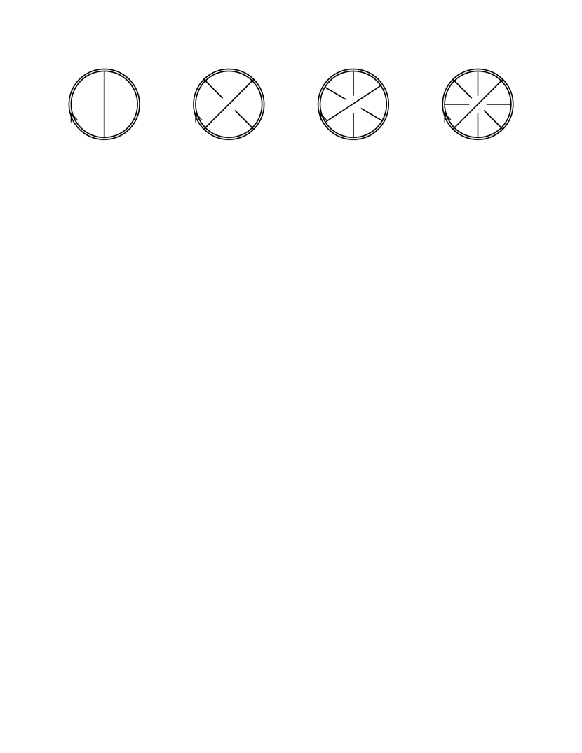
Computing the contribution of three-loop planar diagrams to the vertex function, we performed the numerator algebra using Form Vermaseren:2000nd , TForm Tentyukov:2007mu or Reduce reduce . In this way, we obtained scalar HQET integrals which can be mapped onto the 8 generic topologies 666Counting the number of needed topologies, we made use of the symmetry of under exchange of the heavy quarks, . shown in Fig. 6 either manually or using q2e and exp Harlander:1997zb ; Seidensticker:1999bb .
 |
 |
 |
 |
 |
 |
 |
 |
Applying integration-by-parts identities Chetyrkin:1981qh , the three-loop integrals are then reduced to a set of 71 master integrals with the help of Crusher crusher , Fire Smirnov:2008iw ; Smirnov:2013dia ; Smirnov:2014hma or LiteRed Lee:2012cn ; Lee:2013mka . The evaluation of the master integrals, which plays a central role in the calculation, is described in detail in Section 4. Matching the divergent part of the vertex function to the expected form (16) and (2.2), we obtain the three-loop cusp anomalous dimension given in Section 5. Its properties, which also serve as indispensable checks of our calculation, are discussed in Section 6.
In addition, in the case of QCD, we compute corrections to the cusp anomalous dimension enhanced by the number of fermions, and . The details of the calculation can be found in Appendices C and D.
4 Three-loop calculation of HQET integrals
In this section, we describe our choice of the basis of Feynman integrals that contribute to the cusp anomalous dimension at three loops and present their calculation. An unusual feature of these integrals as compared with the conventional Feynman integrals is that they involve eikonal or heavy quark propagators (see figure 3). In what follows we refer to them as HQET integrals.
In section 4.1, we start by introducing the generalized polylogarithm functions required in our calculation. In section 4.2 we discuss their weight properties and relation to Feynman integrals. To explain the procedure, we first explain our method for computing the master integrals using differential equations. The two-loop case is reviewed as a pedagogical example in section 4.3, Next, in sections 4.4 and 4.5, we explain in detail our choice of integral basis. We give there two complementary points of view, the first being based on analyzing the Wilson line integrals in position space, and the second analyzing generalized cut properties of the same integrals in the momentum-space. Finally, in section 4.6, we perform the three-loop calculation of the master integrals.
4.1 Iterated integrals
We will see below that the HQET integrals required in our calculation can be expressed in terms of certain iterated integrals studied in the mathematical literature Goncharov1 ; Brown1 . More precisely, a particular subclass of such integrals, known in the physics literature as harmonic polylogarithms (HPL) Remiddi:1999ew ; Gehrmann:2001pz , is sufficient to express all results.
The harmonic polylogarithms depend on the set of indices taking values . They are defined iteratively with respect to their weight . The iteration starts with the weight-one functions
| (26) |
For all indices being different from zero, for , higher weight functions are defined as
| (27) |
with the integration kernels
| (28) |
In the case of all indices being zero, we have
| (29) |
The weight of refers to the number of integrations with logarithmic kernels , , and equals the length of the index vector . In the physics literature, it is sometimes colloquially referred to as “transcendentality”.
Iterated integrals satisfy a shuffle algebra, which expresses the product of a weight and a weight function as a sum over weight functions,
| (30) |
where the list of length arises from “shuffling” the lists and , like a deck of cards.
Special values of harmonic polylogarithms at and are related to nested sums, called Euler sums. The latter satisfy additional relations, see e.g. Broadhurst:1998rz ; Remiddi:1999ew , that allow us to reduce them to a minimal number of constants. It turns out that in our calculation, only zeta values are needed.
4.2 Pure functions of uniform weight
In our calculation, functions of uniform weight play an important role. The latter are defined as linear combinations of iterated integrals of the same weight with coefficients rational in . For example,
| (31) |
is a function of uniform weight . We can go further and define so-called pure functions, which are linear combinations of uniform weight functions with rational coefficients, e.g.
| (32) |
Pure functions have nice properties that make them easy to compute. Most importantly, their differential has a simple form. If is a pure function of weight , then
| (33) |
where , the are at most algebraic functions, and are certain pure functions of weight . For example,
| (34) |
For , the expression on the right-hand side of (33) contains only one term, since there is only one (independent) weight zero function . As a consequence, the relation (33) allows for a simple recursive way of defining a weight function, through differential equations. This is precisely the route that we take in section 4.3 below.
Let us imagine we have a set of Feynman integrals that can be evaluated in terms of iterated integrals. Taking certain linear combinations of these integrals, we may try to express them in terms of pure functions. But is there a way to tell in advance which Feynman integrals will evaluate to pure functions?
A proposal in this direction was made in ArkaniHamed:2010gh , based on ideas related to generalized unitarity Bern:1994zx ; Cachazo:2008vp , and relying on a large body of evidence from computations in super Yang-Mills. To understand this, let us imagine a Feynman integral depending on many kinematic variables. Iterated integrals are multivalued functions in these variables. The idea is that taking generalized unitarity cuts of Feynman integrals should in some way correspond to taking discontinuities of these functions (the precise correspondence between the two objects is an open problem). Then, taking different discontinuities should project onto different terms in the expression of an integral in terms of iterated integrals. The conjecture of ArkaniHamed:2010gh is that if all leading singularities (corresponding to a series of cuts that completely localize a Feynman integral) are rational numbers, the answer is a pure function.
This conjecture was verified in a number of non-trivial examples, see e.g. Drummond:2010cz ; Dixon:2011nj . Moreover, it turned out that choosing such integrals as a basis rendered the physical answer much simpler already at the integrand level, before carrying out the integrations. (This is in part due to the close relationship between certain unitarity cuts and infrared divergences, whose appearance is clearer in the new basis choice.)
The understanding of the relationship between Feynman integrals and uniform weight functions was put on a firmer footing in Henn:2013pwa , by providing a way of proving the conjecture with the help of differential equations. It is known that Feynman integrals viewed as functions of kinematical invariants satisfy a system of first-order partial differential equations (see e.g. Argeri:2007up ; Henn:2014qga for reviews). Denoting the set of such integrals by we have in complete generality
| (35) |
where is a nontrivial matrix depending on the dimensional regularization parameter and the differential on both sides is taken with respect to . In Henn:2013pwa it was suggested that by changing the basis to uniform weight functions, the differential equation (35) should take a simple canonical form,
| (36) |
with the matrix being independent and given by a linear combination of logarithms with rational coefficients. We can write a formal solution to (36) as a path-ordered exponential
| (37) |
with some contour connecting the base point at with the function argument, and being the boundary values.
In fact, in the canonical form (36), each term in the expansion of satisfies an equation of the form (33), which allows one to prove that has uniform weight . 777In principle, transcendental constants could enter through the boundary conditions. Experience shows that this does not happen if the basis is chosen according to the criteria explained below. Moreover, assigning weight to , each has uniform weight, in the sense of the expansion.
How does one find an appropriate basis ? Given the conjecture of ArkaniHamed:2010gh , integrals having constant leading singularities in the sense of that paper are a natural choice. The differential equations then allow one to prove the uniform weight properties of those functions. We remark that generalized unitarity cuts are also very natural in the context of differential equations. The reason is that the cut integrals satisfy the same differential equations as the original integrals, but with different boundary conditions. The cuts allow one to focus on a subset of integrals that share a common propagator structure. This can be used e.g. for making consistency checks before the whole system of differential equations is considered.
Another strategy put forward in Henn:2013pwa is to try to deduce the weight properties from an integral representation, e.g. in Feynman parametrization. This works particularly well in cases with few propagators, and for Wilson line integrals. We will present various examples below.888A well-known case where the weight properties of the answer could be deduced from an integral representation is Kotikov:2004er . Based on properties of the BFKL equation, the authors conjectured that the leading weight pieces (the “most complicated part”) of twist-two anomalous dimensions in QCD and supersymmetric Yang–Mills theories should coincide.
4.3 Two-loop master integrals and differential equations
Let us present as an example the full set of differential equations (36) for the two-loop case. The analysis at three loops will be almost identical, except that the system will be much larger. Going through the simple two-loop example therefore allows us to be more explicit.
In order to discuss all planar two-loop integrals (recall that non-planar integrals can be obtained via eikonal identities), we introduce the following notation
| (38) |
where are arbitrary integer indices and
| (39) |
Examining (38) for various values of indices, we identify two families of integrals that match topology of planar Feynman diagrams contributing to the cusped Wilson loop at two loops. They are shown in figure 7(a), (b) and are given by
| (40) |
respectively. All other planar two-loop integrals can be obtained by pinching lines (setting some of the to zero), or adding numerators (setting some to negative values).
Integral reduction using integration-by-parts (IBP) identities Chetyrkin:1981qh shows that there are nine master integrals that can come from the two families of integrals shown in (40). Notice that integral reduction programs automatically choose a particular integral basis according to certain criteria. Such a basis typically does not have the uniform weight properties discussed above, and hence leads to a complicated form of differential equations (35). In order to bring the differential equations to a simple canonical form (36) we make the following choice of master integrals,
| (41) | ||||
| (42) | ||||
| (43) | ||||
| (44) | ||||
| (45) | ||||
| (46) | ||||
| (47) | ||||
| (48) | ||||
| (49) |
where . Here dot denotes a propagator squared in momentum space. A distinguished feature of this basis is that all functions have a uniform weight. This property is by no means obvious and can be established using the methods discussed in subsections 4.4 and 4.5.
All integrals depend on dimensionless kinematical variable
| (50) |
with , and are normalized in such a way that are expected to be pure functions of weight zero. This can be verified by computing their differential with respect to the kinematic variable . Using the definition (50), we can implement this by differentiating the defining Feynman integrals with respect to ,
| (51) |
In this way, we find that the set of nine basis integrals satisfies the differential equation (36)
| (52) |
with and
| (71) |
In order to solve the differential equation (52) we also need boundary conditions. The latter can be easily fixed for , or equivalently , where no singularities are expected from the Feynman integrals. Since in this limit, the only non-vanishing integrals in (41) – (49) are , , and . For they are reduced to integrals with bubble insertions and can be easily evaluated (see relations (86) below). In this way, we find
| (72) |
with all other integrals vanishing at . Making use of
| (73) |
it is easy to see that the above expressions give rise to uniform weight expansions.999This formula also explains why we have chosen the particular normalization factor for -loop integrals, namely to avoid the appearance of in our results.
Returning to the differential equation (52), we can write its solution as
| (74) |
Matching the coefficients in front of powers of on the both sides of (52), we find that are given by a -linear combination of harmonic polylogarithms of weight defined in section 4.1. It is then straightforward to expand to any desired order in . For instance, we have
| (75) |
In agreement with our expectations, the coefficients in front of powers of are pure functions.
We should mention that the basis choice of is not unique. As we show in the next subsection, we can introduce two other integrals
| (76) | ||||
| (77) |
that are also pure functions of weight zero. They are related however, via IBP identities, to the nine basis functions . In order for and to be pure functions, they should be given by a -linear combination (independent of and ) of the basis integrals. Indeed, we find that
| (78) |
This also means that, replacing e.g. by would have lead to an equally nice set of differential equations.
Of course, not all integrals have such nice properties. As an example, consider the following integral that can appear in the Feynman diagram calculation
| (79) |
This integral is obviously not a pure function. Choosing it as a basis integral would lead to an unnecessarily complicated dependence of the differential equations on and .
4.4 Wilson line diagrams in position space and uniform weight integrals
In this and in the following subsection we explain the method that we use to identify integrals that can be evaluated in terms of pure functions.
As a warm up example we revisit the calculation of Wilson line integral (see figure 8(a)) that contributes to the one-loop cusp anomalous dimension. It is given in position space by an integral of a scalar propagator connecting two points and , with and being the line integration parameters,
| (80) |
Using this identity, the integrand can be written in the so-called “d-log”’ form Henn:2013wfa 101010For the time being, we perform the analysis in dimensions, and do not yet specify the range of integration for and .
| (81) |
In this form, it is manifest that the integral, multiplied by , has a differential of the form (33), with , and is hence a pure function of weight two. Likewise, Wilson line integrals with more propagators stretched between two (or more) semi-infinite rays are seen to be pure functions of higher weight. (An algorithm for computing all such contributions was given in ref. Henn:2013wfa .)
The above analysis is rather formal since the Wilson integral is divergent and requires regularization both in UV and IR. As we will see in a moment, regularization does not affect the uniform weight properties of the integral. For example, at one loop the regularized Wilson line integral (8) is given, up to overall factor
| (82) |
Here we changed variables according to , and introduced notation for
| (83) |
with . The integral in (82) gives UV divergence . More generally, introducing as an overall scale in a given Wilson line integral, we can always separate the integration from the rest of the calculation. Moreover, the integral can always be evaluated in terms of gamma function, typically at loops, which does not change the weight properties of the answer, except for an overall offset. Therefore, in the examples below, we will not discuss further the integration.
Let us examine the integral . The integrand in (83) can be Taylor expanded in . At , the integral is obviously evaluates to a logarithm, i.e. a pure weight-one function. It is easy to see that expanding (83) at higher orders in will increase the weight of the resulting function accordingly. With the convention that has weight , we can therefore see that has uniform weight one. We could proceed along the lines of section 4.2 (see also refs. CaronHuot:2011kk ; Henn:2013wfa ) and evaluate the integral, at a given order in . Instead, in this paper, we evaluate all such integrals using differential equations, with as a parameter.
We can show in a similar manner that the integrals with propagators attached to two (or more) semi-infinite rays are expressed in terms of pure functions of weight . Indeed, we can apply the identity (81) to each propagator to deduce that the integral is given by (with ) times a pure function of weight . As in the one-loop case, introducing regularization does not affect this result. 111111There is a small subtlety that the double ladder diagram has a subdivergence, so that strictly speaking we are not allowed to Taylor expand under the integral sign. However, we can avoid this problem by performing the same analysis for the crossed ladder diagram, which is equivalent to the double ladder, up to the one-loop ladder integral squared. For example, at two loops, the ladder integral that enters into the definition (41) of the basis function , is given by the product of and a pure function of weight . Multiplying the ladder integral by we therefore obtain a pure function of weight . This explains the origin of the normalization factors in the definition of .
The above analysis can be generalized to integrals where propagators are raised to some power. For example, consider the integral of figure 8(b) where a dot denotes a propagator squared (in momentum space). Parametrizing the end-point of propagators according to , and (with and similar for ), this leads to (up to an inessential overall factor and terms suppressed by powers of ),
| (84) |
where we denoted . Here the UV pole comes from integration and the additional factor of on the left-hand side comes from the Jacobian of the change of variables and the doubled eikonal propagator. This shows that the integral is given by a function of weight three. We can convert it into a pure function of weight zero by multiplying the integral by the normalization factor . The resulting function coincides with defined in (76).
Another example is the integral shown in figure 8(c). The Fourier transform of the doubled propagator gives , so that this factor is irrelevant at the level of the integrand and can be replaced with . Parametrizing the line integrals as in the previous example, we obtain
| (85) |
We conclude that this integral multiplied by yields a pure function of weight zero. It coincides with the basis function defined in (46).
These examples might mislead the reader in thinking that the uniform weight property is rather trivial. However, this is not the case. For instance, just moving the dot in the above examples to another propagator destroys this property. In our analysis, it would result in the impossibility of rewriting the integrand in a “d-log” form.
For integrals with fewer propagators, bubble subintegrals can appear. Whenever this happens, the latter can be integrated out, leaving one with an integral that effectively has one loop less, up to some gamma functions coming from the integration. This means that many integrals can be chosen based on the knowledge of pure functions at the lower loop order. The relevant formulas are obtained by elementary integrations in Feynman parameter space. For a bubble on an eikonal line (see (42)) and for a scalar bubble (see (43)) we have, respectively,
| (86) |
where and
| (87) |
The momentum dependence of these integrals that is important for the present analysis can be simply obtained by power counting.
We can use the relations (86) to express the two-loop integrals entering the definition of basis functions (42), (43), (45) and (49) in terms of one-loop integrals. Moreover, the bubble-type integrals entering (44) and (48) can be entirely evaluated in terms of functions. In this way, we verify that , , , , and are indeed pure functions of weight zero. 121212 We remark that, in general, whenever bubble integrals are present, one may choose further integrals thanks to possibility of adding a numerator, so that the lower-loop integral has propagators raised to power . Examples of this can be found in Henn:2013tua ; Henn:2014qga . In a certain sense, this phenomenon appears in , since integrating out the sub-integral gives a triangle with one eikonal propagator raised to power .
Let us now discuss the two-loop master integrals with an internal interaction vertex, cf. (47) and (77). It is convenient to analyze them in position space as well. For simplicity, we will carry out the analysis in four dimensions. Let us begin with the integral in (77) and denote by , , the points the three-point vertex is attached to, with , lying on the same Wilson line segment. (For the integral in (47) we can set .) These points can be parametrized by
| (88) |
with and . Consider carrying out the integration over the internal vertex. The integral involves three scalar propagators attached to this vertex and it gives rise in four dimensions to Usyukina:1993ch
| (89) |
where , , , , and is a known pure function of weight two. Its explicit expression is not relevant for the present analysis. The latter focuses on the question whether the integrand can be put in “d-log” form.
Just as in the case of propagator exchanges, there are simplifications due to the fact that the Wilson lines lie in a plane, which leads to simplifications. After some algebra, we find for the integrand (for )
| (90) |
where in the last relation we changed variables as , , . The integration just gives an overall normalization, while the remaining integrand can be put into a “d-log” form. Remembering the weight-two function , we expect that the integral, normalized by , gives a pure weight four function. Then, we multiply it by to obtain a pure function (77) of weight zero.
We can use the calculation above in order to also analyze the integral (47) where . This is simply achieved by setting and dropping the integration in (4.4). In this case, after changing variables according to , we obtain
| (91) |
Notice that the integral is divergent at . If we introduced the dimensional regularization from the beginning, the integrand (91) would be modified by the factor leading to a pole upon integration over . Therefore, as in the previous case, we expect the integral in (47) to be a uniform function of weight four and, as a consequence, the basis function to be a pure function of weight zero.
It is clear that the method discussed in this subsection does not rely on a particular loop order and it proves to be very useful in selecting uniform weight integrals at the three-loop order.
The attentive reader may have noticed that the above analysis relied mainly on the properties of the denominator factors and not those of the function defined in (89). In fact, ignoring this function corresponds to taking a generalized cut, making contact with the conjecture of ArkaniHamed:2010gh . Similarly, and perhaps more easily, we could have taken the maximal cut of this integral in momentum space, with the conclusion that it has a unique normalization factor . As we will demonstrate in the next subsection, the approach based on generalized cuts is especially useful for more complicated integrals with many propagator factors that can be cut.
4.5 HQET integrals in momentum space and maximal cuts
In this subsection, we perform an analysis of maximal cuts of HQET integrals in momentum space. The objective is to determine whether a given integral has a unique overall normalization factor, consistent with being a pure function. We will start by reviewing some of the integrals of the previous subsection, and then turn to an example occurring in three-loop computation.
Let us start by verifying the normalization factor of the one- and two-loop ladder integrals. We work in four dimensions but keep IR regularization with . The maximal cut of the one-loop integral (8) is given by (here and in the remainder of this subsection we will neglect inessential independent normalization factors)
| (92) |
There are various ways of evaluating this integral. To solve the massless on-shell condition for the loop momentum we make use of spinor variables (see, e.g., Dixon:1996wi ) 131313Another way could be to use Sudakov decomposition and carry out integration over , and .
| (93) |
or simply . Together with , this leads to
| (94) |
This is indeed the correct normalization factor, cf. eq. (82). Similarly, a short calculation shows that the maximal cut of the double ladder integral is given by
| (95) |
which is consistent with eq. (41).
Let us now consider a more complicated example of three-loop integral containing propagators shown in figure 9(a).
Its maximal cut is best understood by first evaluating the maximal cut of the one-loop subintegral shown in figure 9(b) (with all external legs cut, i.e. ). The latter is given by
| (96) |
where four delta-functions localize the integral. Applying (96), we effectively reduce the integral of figure 9(a) to a two-loop integral. It contains however two additional propagators coming from the right-hand side of (96) and does not produce a function of uniform weight. We can improve the situation by inserting into the integral of figure 9(a) a numerator factor depending on loop momenta. The latter can be chosen, e.g., to cancel part of the factors coming from (96). In this way we can obtain two-loop integrals that are expected to be of uniform weight based on the analysis of the previous subsection.
Explicitly, inserting the numerator factors and , we evaluate the maximal cut as
| \psfrag{k1}[cc][cc]{$k_{1}$}\psfrag{k12}[lc][cc]{$k_{2}-k_{1}$}\psfrag{k3}[cc][cc]{$k_{3}$}\psfrag{V1}[cc][cc]{$v_{1}$}\psfrag{V2}[cc][cc]{$v_{2}$}\psfrag{num}[cc][cc]{$\otimes(-k_{2}^{2})$}\includegraphics[width=130.08731pt]{hqet_pic13.eps} | \psfrag{x1}[cc][cc]{}\psfrag{x2}[cc][cc]{}\psfrag{x3}[cc][cc]{}\psfrag{x4}[cc][cc]{}\includegraphics[width=86.72267pt]{hqet_pic4.eps} | (97) | |||||
| \psfrag{k1}[cc][cc]{$k_{1}$}\psfrag{k12}[lc][cc]{$k_{2}-k_{1}$}\psfrag{k3}[cc][cc]{$k_{3}$}\psfrag{V1}[cc][cc]{$v_{1}$}\psfrag{V2}[cc][cc]{$v_{2}$}\psfrag{num}[cc][cc]{$\quad\otimes(-2k_{3}\cdot v_{1}+1)$}\includegraphics[width=130.08731pt]{hqet_pic13.eps} | \psfrag{x1}[cc][cc]{}\psfrag{x2}[cc][cc]{}\psfrag{x3}[cc][cc]{}\psfrag{x4}[cc][cc]{}\includegraphics[width=86.72267pt]{hqet_pic8.eps} | (98) |
With this choice of numerator factors, the three-loop integrals have a unique normalization factor and, therefore, they are good candidates for pure functions. This result is not too surprising, given that very similar results were obtained in Henn:2013tua for massless two–to–two amplitudes.
The techniques described in this and the previous subsection allow us to easily and quickly assemble a list of candidate integrals that give rise to pure functions. In the case of the generalized unitarity cut or leading singularity analysis, this is expected based on the conjecture of ArkaniHamed:2010gh . The differential equation method allows us to prove the uniform weight property in the cases where it was only conjectured.
4.6 Three-loop master integrals and differential equations
In this subsection we extend the calculation of HQET master integrals to the three-loop level. As discussed in section 2.4, thanks to eikonal identities we need to calculate only planar HQET integrals. To this end, we define all planar integral families at three loops, describe the choice of master integrals and their computation via differential equations. Due to the size of the matrices involved, unlike the two-loop case, we select not to present the latter in this paper, but provide them and other results in the form of ancillary text files.
4.6.1 Definition of master integrals
All planar three-loop HQET integrals can be viewed as some special cases of the integral families shown in figure 10. Thanks to planarity it is possible to describe all of them using a global parametrization of the loop momenta . In order to do so, we define the following factors,
| (99) |
We then introduce the following notation for the HQET integrals,
| (100) |
The integral families shown in figure 10 correspond to the following expressions in the notation of (100) (more generally, the indices can of course be different from ),
Numerator factors can be accommodated by negative values of the indices . It is worth pointing out that the labeling in is not unique, in the sense that the same integrals can be represented by different index vectors. This is due to invariance under relabeling of loop momenta, due to symmetry of some graphs and due to a symmetry of the integrated results.
We remark that with the above setup we can also discuss factorized integrals. In particular, one-loop integrals multiplying generic two-loop integrals can be treated as a subset of the three-loop integrals. This is a useful check, and also allows for a convenient calculation of, say, higher orders of their expansion, within the same setup.
Solving the IBP relations for integrals shown in figure 10, we find that there are master integrals in total. We choose the master integrals according to the uniform weight criteria explained in detail in subsections 4.4 and 4.5, following Henn:2013pwa . We denote the basis integrals by , hoping that using the same letter that we previously used to denote two-loop basis integrals with will not lead to confusion. As in the two-loop case, all basis three-loop integrals are pure functions of of weight zero. All except a handful of integrals could be chosen to be given by a single master integral (100), with certain powers of propagators, and normalized appropriately. Only in a few cases it turned out to be necessary to consider linear combinations of integrals (100). 141414Expressions for the basis integrals in terms of master integrals (100) can be found in the ancillary file HQET_3loop_basis_f.m in the arxiv submission of this paper.
4.6.2 Integral subsector at three loops
As an example of the basis integrals at three loops, let us to return to three-loop integrals discussed in subsection 4.5 (cf. eqs. (97) and (98)). In the notation of eq. (100) they read
| (101) | ||||
| (102) |
We can use them to illustrate the relationship between generalized cuts and projections onto sectors of the differential equations.
Let us consider the maximal cut of these integrals, i.e. replace all scalar and eikonal propagators with their cut version, and denote the resulting integrals by and . The latter satisfy a closed system of differential equations. This system of two equations is a subset of the full system of equations. This follows from the fact that cut integrals satisfy the same IBP relations as standard ones Anastasiou:2002yz . Another way of saying this is that cut integrals satisfy the same differential equations as the standard integrals, but with different boundary conditions (in particular, the remaining basis integrals vanish upon taking the above mentioned cut, for ). This means that the subsystem of basis integrals (101) and (102) is relevant for the full calculation. In particular, it can serve as a check of whether the choice (101) and (102) is consistent with the canonical form (36) of the differential equations.
Indeed, we find that the integrals (101) and (102) satisfy the system of differential equations,
| (103) |
which is consistent with (36). Of course, removing the cut, it could be that terms violating the form (36) are present in off-diagonal terms. If this is the case, one can attempt to remove them using the methods discussed in ref. Caron-Huot:2014lda and more recently in Henn:2014qga ; Lee:2014ioa . It turns out that this is not needed for the two integrals under discussion. In our calculation, we resorted to such “brute-force” methods only in the case of a handful of integrals.
4.6.3 Full system of differential equations
With the basis given in ancillary files included in the arxiv submission of this article, the differential equations take the form
| (104) |
with constant matrices , and given in the ancillary file HQET_3loop_mAtilde.m.
We see that eq. (104) has four regular singular points, , , , . Due to the symmetry of the definition (50), only the first three are independent. They correspond, in turn, to the light-like limit (infinite Minkowskian angle), zero angle limit and backtracking limit.
As before, we can solve eq. (104) in a Laurant expansion (74). Then we can express order by order in in terms of harmonic polylogarithms. We use the value of basis integrals at as boundary condition Grozin:2000jv ; Chetyrkin:2003vi (see Grozin:2008tp for a summary).
Most of the basis integrals can be evaluated trivially for in terms of Gamma functions. Boundary conditions for Feynman integrals can often be obtained without additional work, by imposing physical properties. In reference Henn:2013nsa this was used e.g. in a bootstrap approach to compute single-scale integrals from differential equations. In the present case, we can use finiteness of the limit as our main condition. It turns out that only one non-trivial integral is needed at . It is known up to weight five Czarnecki:2001rh (but this is the order we are interested in),
| (105) |
which is exactly the order we need for our calculation. It is likely that also this integral could be obtained by inspecting the differential equations more closely, or applying bootstrap ideas as in Henn:2013nsa .
4.6.4 Solution
As noted above, the solution to (104) to any order in is expressed in terms of harmonic polylogarithms. The explicit expressions for basis integrals up to weight five can be found in the ancillary file HQET_3loop_HPL.m.151515A curious feature is that integral is apparently finite as and a weight six function, and therefore appears only at order in our normalization. As an example, we have
| (106) |
We remark that the differential equation, or equivalently, the path integral (37) encodes all the information about the symbol Goncharov1 ; Brown1 ; Brown2 ; Goncharov:2010jf of the result (and all possible symbol related simplifications are already manifest). The latter can immediately be computed as a corollary. In order to do this, in addition to the matrix , only the leading term in expansion (74) is required. The latter reads
| (107) |
We have evaluated all basis integrals using Fiesta Smirnov:2013eza at the value and found perfect agreement with analytical formulas, within the error bars.
There are a number of analytic checks. Out of master integrals, are straight-line ones (studied in Grozin:2000jv ; Chetyrkin:2003vi ), can be chosen as products of lower-loop integrals, and correspond to the one-loop triangle integral with -dependent powers of denominators (studied in Grozin:2011rs ). One non-trivial integral at was obtained in our approach from the finiteness of the limit for all integrals entering the differential equations. Previously, it was computed in terms of a hypergeometric function in ref. Beneke:1994sw (another hypergeometric representation was derived in Grozin:2008nu ). We can expand it in using the Mathematica package HypExp Huber:2005yg . The result, written up to weight five, is
| (108) |
We found perfect agreement with our result.
4.6.5 Check of supersymmetric Wilson loop in SYM
We can also perform analytic checks of our results by comparing to the supersymmetric cusped Wilson loop (4) in super Yang–Mills theory,161616In this section, for simplicity of presentation, we choose the Wilson loop (4) to be in the fundamental representation, , and we take the planar limit, corresponding to .
| (109) |
It was computed at three loops in ref. Correa:2012nk , using a different method. This quantity depends on two cusp angles and and the dependence on the latter angle enters through the following variable
| (110) |
Up to three loops, the perturbative corrections to can be expressed in terms of master integrals defined in (38) and (100) 171717Strictly speaking, the calculation in ref. Correa:2012nk was performed for in which case .
| (111) |
where .
Using the obtained results, we reproduce results of the three-loop computation performed in Correa:2012nk . For example, the following three-loop integral was computed there (taking into account the conversion between the different regulators),
| (112) |
In terms of the three-loop basis integrals defined above it reads
| (113) |
Using the explicit results for and we found full agreement with (112) (note that the individual results for and are rather complicated in comparison). In the similar manner, we reproduce the remaining three-loop integrals
| (114) |
where .
We can use the above results to compute the three-loop cusp anomalous dimension for the supersymmetric Wilson loop in super Yang–Mills theory
| (115) |
In perfect agreement with findings of ref. Correa:2012nk , we find
| (116) |
with and given by (110). This is a highly nontrivial test of the calculation of the master integrals. Within the differential equations method, the calculation of a given integral requires the knowledge of all integrals appearing in sub-topologies (obtained by removing propagator factors). Since the integrals needed here have a maximal number of propagator factors, this calculation is also a consistency check of many other integrals appearing for example in QCD.
5 Results
The basis integrals defined in the previous section allow us to compute the cusped Wilson loop (16). For example, we can express the three-loop correction to as
| (117) |
where are coefficient functions rational in and depending on . Their explicit form is not particularly enlightening. We can write similar formulas for and . 181818As was already mentioned, the three-loop integrals computed here can also be used to express all required one- and two-loop integrals, by writing the latter as factorized three-loop integrals, where the additional factors are trivial. Then, we extract divergent part of and match it into expected form (2.2) of . In this way, we verify gauge independence of factor, reproduce well-known result for function and extract the three-loop cusp anomalous dimension.
5.1 Coefficient functions
To express our results for three-loop cusp anomalous dimension we introduce the following functions
| (118) | ||||
where we recall that and . The subscript of and indicates the (transcendental) weight of the functions.
The three-loop cusp anomalous dimension involves particular linear combinations of these functions
| (119) |
and
| (120) |
As follows from the definition, these functions vanish for zero cusp angle, or equivalently .
5.2 Three-loop cusp anomalous dimension
In QCD with fermion flavours, we obtained the following result for the three-loop cusp anomalous dimension (13) in the scheme
| (121) |
where and are the quadratic Casimir operators of the gauge group in the fundamental and adjoint representation, respectively, and for fermions in the fundamental representation. The relation (5.2) involves the coefficient functions defined in (119) and (120).
In the gauge theory with fermions and scalars in the adjoint representation of the , the three-loop cusp anomalous dimension is given by
| (122) |
with the same coefficient functions (119) and (120). Denoting this expression as , we can get the three-loop cusp anomalous dimension in supersymmetric Yang–Mills theories with different number of supercharges by adjusting the number of fermions and scalars
| (123) |
In section 6.2, we will also give the result for in the dimensional reduction scheme.
A close examination of (5.2) and (120) shows that the coefficients describing and -dependent contribution at three loops, involve the same functions , and that already appeared at two loops. This suggests that these coefficients are not independent. Indeed, we show in the next section that the cusp anomalous dimension has an interesting hidden structure that allows us to predict all and -dependent terms at three loops at least.
Notice that all functions in (118) except depend on and, therefore, they are formally invariant under . However, due to the presence of the cut that runs along negative , these functions acquire an additional contribution under proportional to their discontinuity across the cut (see (25)). For the function the situation is slightly different. The linear combination of harmonic polylogarithms inside the brackets in formally changes the sign under . It is compensated however by the odd prefactor , so that has the same parity properties as the other coefficient functions. In this way, we verify that our results for three-loop cusp anomalous dimension (5.2) and (5.2) satisfy the relation (25).
6 Properties of the cusp anomalous dimension
6.1 Casimir scaling
Let us discuss the dependence of the cusp anomalous dimension on the color factors. These factors appear as a result of manipulation with traces involving the generators of various representations. More precisely, in the case of QCD we encounter the generators of three different representations: fundamental for fermions , adjoint for gluons and, in addition, some arbitrary representation that enters into the definition (1) of the cusped Wilson loop. In the case of SYM, the generators in the fundamental representation do not appear since all fields are defined in the adjoint of the .
We observe from (5.2) that the dependence of the three-loop cusp anomalous dimension on the representation enters through an overall factor given by the quadratic Casimir of this representation , the so-called Casimir scaling
| (124) |
with being independent of . As was already mentioned in section 2.4, we expect this scaling to be broken at four loops due to appearance of higher Casimirs.
To understand this property, let us examine possible color factors that can appear in the perturbative expansion of Wilson loop (1) up to four loops. To simplify the analysis we first examine supersymmetric Yang–Mills theory. The color factor in this case consists of terms having the form with each corresponding to a gluon attached to the integration contour. The tensor is a product of and factors.191919 There exists no subset of without external indices (such a subset would correspond to a vacuum subdiagram). So, there always exists a factor directly contracted to the trace of . Substituting , we transform such terms into the sum of two terms having less factors (but more factors inside the trace). Applying this procedure recursively, we finally reduce any color factor to a linear combination of terms of the same form where all tensors are products of only. In this way, we obtain the basic color factors shown in figure 11.
The remaining color factors can be reduced to products and sums of the basic ones. Going through the calculation we find
| (125) |
where is the dimension of the representation and with being the quadratic Casimir of the adjoint representation of . An important difference of compared to (125) is that it cannot be expressed in terms of quadratic Casimirs only. More precisely, its takes the form
| (126) |
where the ellipsis denotes terms involving quadratic Casimirs and . Here and are fully symmetric tensors
| (127) |
with the generators defined in two different representations.
The color factors appear in the expression for the cusp anomalous dimension starting from loops. The very fact that (126) is not proportional to the quadratic Casimir for the generic representation implies that the Casimir scaling (124) should be violated at four loop unless some miraculous cancellation happens leading to the vanishing (angle dependent) coefficient function accompanying .
Notice that the color factors (125) contain higher power of . As we explained in section 2.4, in virtue of nonabelian exponentiation, the cusp anomalous dimension should involve maximally nonabelian factors only. Up to three loops they take the form , and . This means that the cusp anomalous dimension depends on particular combinations of the color factors, , and . At four loops, the maximally nonabelian color factors are of two kinds, and . The latter color factor leads to a violation of the Casimir scaling (124) at four loops and induces a nonplanar correction to the cusp anomalous dimension.
Let us now consider the color factors in QCD. An important difference with the previous case is that the fermions are defined in the fundamental representation. This leads to the appearance of additional color factors proportional to the number of fermion flavours . Each fermion loop produces a factor of and the maximal power of scales with the loop order. In particular, the color factors linear in have the form , with the tensor being given by a product of Kronecker symbols. As in the previous case, up to three loops -dependent color factors can be expressed in terms of quadratic Casimirs , and , where is the quadratic Casimir of the fundamental representation of . Most importantly, the additional dependence does not affect the Casimir scaling (124) at three loops but it modifies the form of the function . At four loops, we encounter the color factor analogous to (126), with the completely symmetric tensor given by (127) in the fundamental representation. As before, it is not proportional to and, therefore, leads to violation of the Casimir scaling.
To summarize, the general expression for the four-loop contribution to the cusp anomalous dimension violating the Casimir scaling is
| (128) |
where and are some functions of the cusp angle depending on the choice of the gauge theory. Here the second term inside the brackets is present only if fermions are defined in the fundamental representation, e.g. in SYM. In the special case of being the fundamental representation of the , we have
| (129) |
with . Since these color factors involve various powers of , the expression on the right-hand side of (128) generates nonplanar corrections to the cusp anomalous dimension.
6.2 Renormalization scheme change
We recall that the three-loop calculation of the cusp anomalous dimension has been performed using dimensional regularization (DREG). However supersymmetry is broken in DREG since for the number of bosonic and fermionic degrees of freedom do not match for . To restore the supersymmetry, we can employ dimension reduction (DRED) Siegel:1979wq . In this scheme the gauge fields have four components in dimensions and the difference with DREG comes from the contribution of additional components of the gauge field, the so-called -scalars. Since the number of scalars is a free parameter in our calculation, we can easily accommodate the contribution of -scalars by replacing .
Additional complications arise due to necessity to introduce evanescent coupling constants describing the self-interaction of -scalars and their coupling with fermions. In a generic gauge theory, the renormalization group evolution of the evanescent couplings differs from that of the gauge coupling and, therefore, they have to be treated differently. However, in a supersymmetric theory the beta-functions of these two sets of coupling necessarily coincide allowing us to identify them at any scale. In this case, to compute the cusp anomalous dimension in the scheme it suffices to replace in expression (2.2) for the factor in the scheme, identify the residue at the pole and take into account the relation between the coupling constants in the two schemes Harlander:2006rj
| (130) |
for fermions in the fundamental representation, and
| (131) |
for fermions in the adjoint representation. Notice that scalars do not contribute to (131) at three loops. This leads to the following relation for the cusp anomalous anomalous dimension in the two schemes
| (132) |
In the special case of SYM theory, for and , we use the relations (131) and (132) together with (5.2) to find the three-loop cusp anomalous dimension in scheme
| (133) |
This confirms a conjecture made in our previous paper Grozin:2014hna .
6.3 Asymptotics for large cusp angles
To examine the limit of large Minkowskian angles, we substitute , or equivalently , and put . In this limit, the cusp anomalous dimension is expected to have a logarithmic behaviour Korchemsky:1985xj ; Korchemsky:1991zp
| (134) |
with the so-called light-like cusp anomalous dimension.
We use (5.2) to find at three loops in QCD
| (135) |
We verify that this expression is in perfect agreement with the known result Korchemsky:1987wg ; Moch:2004pa .
In a similar manner, we obtain an analogous expression in a supersymmetric Yang-Mills theory, with fermions and scalars in the adjoint representation, and, then, convert the result into the scheme with a help of (131) to get
| (136) |
To obtain from this expression the three-loop light-like cusp anomalous dimension in SYM, we adjust the parameters following (123),
| (137) |
in agreement with Kotikov:2004er .
6.4 Universal scaling function
We can use the large angle asymptotics of the cusp anomalous dimension (134) to introduce a new effective coupling constant : 202020It is also known in QCD literature as physical coupling constant Catani:1990rr .
| (138) |
Inverting this relation we can expand the cusp anomalous dimension in powers of and define the following function
| (139) |
where and are evaluated in the same scheme. The expansion coefficients of the two functions are related to each other as
| (140) |
with being the coefficients of the expansion of in powers of . According to (132), the change of the renormalization scheme (from to ) amounts to a finite renormalization of the coupling constant. An immediate consequence of (132) is that the coefficients are the same in the two renormalization schemes. This is not the case however for the expansion coefficients of the cusp anomalous dimension, and .
Let us first compute the function in SYM. Using (133) and (137), we obtain from (140)
| (141) |
By construction, this function takes the same form in and schemes.
Similarly, we can apply the relations (5.2) and (6.3) to compute the corresponding function in QCD and in a generic Yang–Mills theory containing fermions and scalars. Since the cusp anomalous dimension depends on the particle content of the theory, we should expect to find different results for . Using the obtained results for the cusp anomalous dimension, we found that the function is independent on the number of fermions and scalars!
This remarkable property immediately implies that, at least to three loops, the function is the same in any gauge theory,
| (142) |
Combining this relation with (140), we conclude that all and dependent terms in are generated from lower-loop terms through expansion of in powers of . It would be interesting to elucidate the origin of the relation (142) as well as its validity beyond three loops.
We would like to mention that similar phenomenon has been also observed in other supersymmetric Yang-Mills theories. In particular, various quantities in three-dimensional supersymmetric ABJM theory Gromov:2008qe and in superconformal Yang-Mills theory Mitev:2014yba ; Mitev:2015oty can be obtained from their counter partners in SYM by replacing the coupling constant by the universal ‘effective’ coupling.
Let us examine the properties of the function .
In the large angle limit, for with , we combine together (134) and (139) to see that has universal asymptotic behavior
| (143) |
where the coefficient in front of the logarithm does not receive corrections and is one-loop exact, that is for . Matching this relation into (141), we find that the linear combinations of and functions that appear in the expansion of at two and three loops remain finite in the large angle limit.
In the small angle limit, for , the integration contour in figure 1 reduces to the straight line leading to the vanishing of the cusp anomalous dimension. For small cusp angle we expect that
| (144) |
where is an analog of the bremsstrahlung function (22). We use (141) to obtain the three-loop result
| (145) |
As before this function takes the same form in any gauge theory (at three loops at least) and does not depend on the choice of the renormalization scheme.
Substituting (144) into (139) we find for the bremsstrahlung function (22)
| (146) |
Then, we use the obtained three-loop results (145) and (6.3) to get in QCD
| (147) |
The two-loop correction to agrees with Korchemsky:1987wg ; Korchemsky:1991zp , the three-loop result is new. In SYM we find from (146) and (137)
| (148) |
6.5 The relation to the quark-antiquark potential
As another check of our results, let us consider the limit with , or equivalently . In this limit, the two rays forming the cusp become anti-parallel and the one-cusp anomalous dimension (14) develops a pole . It is expected that the cusp anomalous dimension should have the same behaviour up to three loops, whereas at four loops it receives corrections of the form 212121It is interesting to note that for the locally supersymmetric Wilson loop similar corrections appear in the cusp anomalous dimension already at two loops Erickson:1999qv ; Pineda:2007kz .
| (149) |
with depending on the renormalization scheme.
As before, it is convenient to examine the asymptotic behavior of the universal function . Indeed, we find from (141) that it develops a pole at three loops
| (150) |
We note that this relation comes about as a result of nontrivial cancellation of more singular contributions coming from various terms in (141). See discussion in section 5.
We substitute (150) into (140) and use the three-loop result for the light-like cusp anomalous dimension (6.3) and (137) to verify that the cusp anomalous dimension satisfies (149) in QCD and in SYM. The corresponding functions are given by
| (151) | ||||
| (152) |
Let us compare the relation (149) with an analogous expression for color-singlet contribution to the static potential of two heavy color sources carrying the charge in generic Yang-Mills theory. In the momentum representation, it has the form
| (153) |
where the function depends on the coupling constant normalized at the scale
| (154) |
with the expansion coefficients and known both in QCD Peter:1996ig ; Peter:1997me ; Schroder:1998vy and in SYM Prausa:2013qva . In the coordinate representation, the potential is given by
| (155) |
with and is proportional to the beta-function
| (156) |
As was observed in Kilian:1993nk , the one-loop correction to (151) coincides with analogous correction to heavy quark-antiquark static potential (154) in QCD, i.e. . Of course, the coincidence is not accidental and can be understood in the conformal limit of QCD.
Namely, for small we can define a conformal transformation that maps two almost antiparallel semi-infinite rays, shown in Figure 1 for , into two (infinite) lines separated by distance . To show this, we assume that the cusp point is located at the origin and introduce the radial and angular coordinates , with and , so that the metric takes the form
| (157) |
where in the last relation we took and introduced new coordinates and . As follows from the last relation, the transformation is conformal at small .
If the conformal symmetry were exact, as it happens in SYM theory, the conformal transformation would allow us to identify the Wilson loops evaluated in two different configurations, thus leading to the expected relation between the cusp anomalous dimension (149) and the static potential (155) for
| (158) |
Note that, in virtue of conformal symmetry, the coupling constant does not depend on the renormalization scale, , and, in addition, in (155).
In the case of QCD, the conformal symmetry is broken by a nonzero beta function. As a consequence, the Wilson loop receives additional, conformal symmetry breaking corrections under the transformation which generate the difference between the cusp anomalous dimension and the static potential in QCD. Since these corrections are necessarily proportional to the beta-function, we expect that the difference between (149) and (155) (for ) should be also proportional to , see e.g. Braun:2003rp . 222222The situation here is similar to that for the Crewther relation in QCD. The conformal symmetry breaking corrections to this relation have been studied in Kataev:2010du ; Kataev:2014zha
Notice that the expansion of the cusp anomalous dimension (149) and the static potential (155) runs in powers of coupling constant normalized at different scales, and , respectively. In agreement with our expectations, the difference between the two couplings is proportional to beta-function multiplied by logarithms of the ratio of the two scales. Choosing we can eliminate such logarithms and arrive at the following relation 232323We did not include into this relation since, by definition (156), this function is proportional to beta-function and, therefore, can be absorbed into .
| (159) |
with and being some function of the coupling constant.
The relations (158) and (159) can be tested using the known two-loop result for the static potential (154) in SYM Prausa:2013qva and in QCD Peter:1996ig ; Peter:1997me ; Schroder:1998vy . Replacing by its expressions (151) and (152), we verified the relations (158) and (159) and identified the lowest order correction to in the scheme
| (160) |
where term depends on at four loops. 242424The simple form of relation (159) suggests that there should exist another, direct way of computing the conformal anomaly for the cusped Wilson loop in the limit.
It was found in Smirnov:2008pn ; Anzai:2009tm ; Smirnov:2009fh that the three-loop correction to the static potential involves higher Casimirs defined in (129). As we argued in section 6.1, the same happens for the cusp anomalous dimension (128) at four loops. Applying (159) we can relate the corresponding terms order-by-order in the coupling. In particular, assuming that the two-loop correction to (160) does not involve higher Casimirs, we can use (159) to predict the four-loop correction to proportional to higher Casimirs in limit. Together with (128) this leads to the following asymptotic behavior of the functions and for
| (161) |
with the numerical coefficients and obtained in Smirnov:2008pn ; Anzai:2009tm ; Smirnov:2009fh by direct Feynman diagram (numerical) calculation
| (162) |
6.6 Nonplanar corrections at four loops
We recall that nonplanar corrections first appear in at four loops and have the general form (128). Applying (140) we can relate them to nonplanar correlations to the function and to the light-like cusp anomalous dimension (138)
| (163) |
with .
In general, four-loop nonplanar corrections and have the same form as (128) and are given by a sum of two higher Casimirs. Notice that one of the Casimirs is accompanied by the factor of . Assuming that (142) is valid at four loops, we find that should be independent and, therefore, involve only one Casimir leading to
| (164) |
with and independent of the cusp angle as well as of the number of flavours . Substituting these relations into (163) and matching the resulting expression into (128) we obtain
| (165) |
Since does not depend on , we can fix its value by examining the asymptotic behavior of the both sides of the last relation for . Taking into account (161) together with we get
| (166) |
with given by (162). This leads to the following prediction for the dependent part of nonplanar correction (128) to the cusp anomalous dimension
| (167) |
In distinction with , the expression for in (165) involves in addition the function defined in (164). Although the explicit form of the function is unknown, we can use (164) and (165) to deduce some of its properties. Namely, examining the asymptotic behavior of both sides of the first relation in (165) for with we find that this function has to satisfy
| (168) |
In addition, in the large angle limit, for with , it follows from (143) and (164) that should stay finite in this limit leading to . This property excludes the possibility for to be proportional to .
6.7 Comparison with the supersymmetric cusp anomalous dimension
It is instructive to compare (133) with the analogous result for the supersymmetric Wilson loop (4)
| (169) |
with , and defined in (4.6.5). In comparison with (133), this expression depends on the internal cusp angle on .
The dependence enters into (4.6.5) through given by (110). For we find
| (170) |
leading to , and . In this way, we arrive at
| (171) |
Recalling that , we observe that this expression involves the same coefficient functions as (133). However, in distinction with (133), it does not vanish for but for , or equivalently . Then, defining
| (172) |
we find
| (173) |
It is interesting to analyze the properties of the terms on the right-hand side of this equation.
First of all, in the light-like limit , they have to give a finite limit, since the scalar coupling to the supersymmetric Wilson loop (4) is suppressed in this limit. Indeed, we observe that , , and all go to constants or vanish in this limit. Second, by definition, they are also well-behaved in the small angle limit, where they modify the coefficients in the Taylor expansion. Third, the limit of the backtracking Wilson line is more interesting. At two loops, the function has a term , which is required to cancel a corresponding term in . Such terms are present in the supersymmetric Wilson line operator at two loops due to certain ultrasoft effects, but not in the case of the bosonic Wilson line operator. Likewise, at three loops, the functions and are required to cancel , , and terms not present in the final result. Finally, the function just contributes a term in this limit.
7 Conclusions
In this paper, we computed the angle-dependent three-loop cusp anomalous dimension in QCD and in a supersymmetric Yang-Mills theories. The obtained expressions are rather compact and are given in terms of harmonic polylogarithmic functions that can be readily evaluated numerically. We discussed in detail special physical limits of the cusp anomalous dimension and, in particular, placed special emphasis on the backtracking Wilson line limit that is related to the quark-antiquark potential. We showed that this relation holds in QCD up to a conformal symmetry breaking corrections proportional to the beta function and identified the leading contribution to the conformal anomaly. It would be interesting to investigate whether the latter can be computed from the first principles.
We found that, unexpectedly, the results for the different theories considered are very similar. In fact, up to three loops at least, they can be written in terms of a single universal function evaluated at an effective charge given by the light-like cusp anomalous dimension. Assuming that this property holds at higher loops, we derived the contribution of the -dependent term that violates Casimir scaling and produces a nonplanar correction to the cusp anomalous dimension at four loops.
Acknowledgements
A.G.’s work was supported by RFBR grant 12-02-00106-a and by the Russian Ministry of Education and Science. J.M.H. is supported in part by a GFK fellowship and by the PRISMA cluster of excellence at Mainz university. G.P.K. is supported in part by the French National Agency for Research (ANR) under contract StrongInt (BLANC-SIMI-4-2011). P.M. was supported in part by the European Commission through contract PITN-GA-2012-316704 (HIGGSTOOLS).
Appendix A Definition of Yang–Mills theories
Throughout the paper, we consider two Yang–Mills theories with different particle content.
In the first case, for gauge fields coupled to species of Dirac fermions, we have
| (174) |
where and with being the generators of the fundamental representation of the normalized as
| (175) |
The fermion fields are defined in the fundamental representation of the and carry the additional flavour index , …, .
In the second case, for gauge fields coupled to scalars and fermions, we have
| (176) |
where is the covariant derivative in the adjoint representation and all fields are matrix-valued in the group, with the generators defined in (175). The scalar fields and the two-component Weyl fermions, and (with , , ), carry the additional flavour index , …, and , …, , respectively. In the second line of (176), the Yukawa coupling involves the matrix .
The reason for choosing the Lagrangian in the form (176) is that, by fine tuning the number of fermions and scalars, we can use it to describe supersymmetric Yang–Mills theories with different number of supercharges. In particular, the maximally supersymmetric Yang–Mills theory corresponds to the special case of (176) with , and matrices (with , …, ) given by (chiral blocks of) Dirac matrices in six-dimensional Euclidean space, (see Appendix B in ref. Belitsky:2003sh for details).
Appendix B Wilson lines and HQET
Wilson lines can be conveniently studied using the heavy quark effective theory.252525Methods of calculation of multiloop Feynman diagrams in HQET are reviewed, e.g., in Grozin:2004yc ; Grozin:2003ak ; Grozin:2008tp ; Grozin:2013bva . In fact, the HQET Lagrangian was first introduced as a technical device for this purpose Gervais:1979fv ; Arefeva:1980zd .
The heavy quark effective fields and depend on the unit four-vector which has the meaning of the heavy quark velocity. The correlation function of two HQET fields (figure 12(a)) is
| (177) |
where and is the projection of onto the subspace orthogonal to . Also, is the expectation value of the Wilson line evaluated along the segment of length oriented along .
It is convenient to work in momentum space. Introducing the notation for the Fourier transformed HQET field
| (178) |
with being the so-called residual energy of heavy quark, we find from (177)
| (179) |
Expanding in powers of the coupling constant yields Feynman diagrams shown in figure 3 for .
Within the HQET framework, the cusp anomalous dimension can be identified as anomalous dimension of the local gauge-invariant operator
| (180) |
To see this, we consider the correlation function of two HQET fields and the current (180)
| (181) |
where stands for the component of orthogonal to and is the expectation value of Wilson line evaluated along two segments of lengths and separated by a cusp angle (see figure 12(b)). In particular, for , or equivalently , we have
| (182) |
Going to the momentum space, we obtain
| (183) |
where and are the residual energies, is the propagator of the HQET field (179) and is the one-particle irreducible vertex function (without the external-leg propagators). For the vertex function coincides with in (16) and is given by Feynman diagrams shown in figure 2.
It is convenient to extract the renormalization factor from
| (184) |
Note that should be gauge invariant and independent on and . In order to avoid infrared divergences, and should be different from zero. It is convenient to choose . Then, the dependence of the HQET integrals on can be trivially obtained by dimension counting. To simplify the calculation, we can set and evaluate the resulting dimensionless integrals in dimensions. The cusp anomalous dimension can be found by matching into the expected result (2.2).
At we find from (182) that the vertex function satisfies the Ward identities
| (185) |
As a consequence, UV divergences of match those of the heavy quark propagator (179) leading to
| (186) |
where is the renormalization factor for the HQET field . Note that is not gauge invariant; at three loops it has been calculated in Melnikov:2000zc ; Chetyrkin:2003vi . We reproduced this result from our three-loop calculation of by setting and using (186).
Appendix C Abelian large- terms
In this appendix, we compute the special class of QCD corrections to the cusp anomalous dimension (20) of the form and . They originate from QED like diagrams which have the form of the one-loop diagram shown in figure 3(a) with a free gluon propagator dressed by fermion loop corrections (see figures 13(a) and (b)). 262626Starting from order, we also have to take into account the additional abelian diagrams shown in figure 13(c). They involve the light-by-light scattering and their calculation is more involved compared to the diagrams shown in figures 13(a) and (b).
To compute the contribution of such diagrams it is sufficient to consider QED with massless lepton flavors. In this case, we put , and treat the one-loop beta-function
| (187) |
as a large parameter. Then, the above mentioned corrections take the form and . We shall refer to them as the leading (L) and next-to-leading (NL) large- corrections, respectively.
For our purposes we need the expression for the photon self-energy with the NL accuracy
| (188) |
Here the leading term comes from the diagram shown in figure 14(a)
| (189) |
where is a bare QED coupling constant. The diagrams shown in figure 14(b) produce the next-to-leading correction to (188). It can be written in the form PalanquesMestre:1983zy ; Broadhurst:1992si
| (190) |
where the function is given by
| (191) |
with the Euclidean integral (with )
that can be expressed via a hypergeometric function of unit argument Kotikov:1995cw ; Broadhurst:1996ur .
The function is regular at the origin and admits a double series expansion
| (192) |
with the coefficients that can be calculated to any order in terms of multiple values. For , the function reduces to Euler gamma functions Broadhurst:1992si (the same holds for ). To save space, we do not presentan explicit expression for .
It is convenient to introduce the renormalized coupling constant
| (193) |
In the large limit, we keep fixed and use as an expansion parameter. In the scheme the renormalized coupling is defined as
| (194) |
where is a bare coupling constant and the charge renormalization constant is given with the NL accuracy by
| (195) |
Here expansion of starts from , that of from , etc. The charge renormalization constant satisfies the renormalization group equation that allows us to express in terms of beta-function.
In the abelian theory, is related to the photon self-energy (188) expressed in terms of renormalized coupling constant
| (196) |
Substituting (188) and (195) into this relation and equating the coefficients in front of on the both sides, we find that in (195) is given by the coefficient of in . It is convenient to choose the renormalization scale as
| (197) |
Then, we use (190) to obtain . Expanding in powers of and replacing with (192), we find that all coefficients but cancel leading to
| (198) |
We can use this relation to find the function with NL accuracy PalanquesMestre:1983zy ; Broadhurst:1992si
| (199) |
Finally, we substitute into the last relation in (196) and obtain correction to the charge renormalization constant (195)
| (200) |
We are now ready to determine the cusp anomalous dimension at the NL order. To this end, we have to repeat the one-loop calculation of the vertex function (see (8) for ), with a free photon propagator modified by self-energy corrections
| (201) |
and, then, express the result in terms of the renormalized coupling constant (193). Performing the calculation we obtain
| (202) |
where the coupling constant is defined at the scale , the function is given by (192) and the notation was introduced for
| (205) |
The function is regular at the origin:
| (206) |
In particular, for we have
| (207) |
The cusp anomalous dimension is related to the residue at the pole in the expression (202)
| (208) |
Replacing in (202) with its general expression (206), we find that the coefficient in front of on the right-hand side of (202) only depends on the coefficients . Then, at the NL order the cusp anomalous dimension is given by
| (209) |
Replacing the coefficients and by their explicit expressions, we finally obtain
| (210) |
This expansion can be extended to any number of loops. The leading term has been derived in Beneke:1995pq , the result for is new. The first term in the expression for is in agreement with our result for in (120).
In a similar manner, we can use (186) to compute the anomalous dimension of the HQET field
| (211) |
where denotes the residue at the simple pole in the expression for . Performing the calculation, we find in Landau gauge at the NL order
| (212) |
The L result has been derived in Broadhurst:1994se . The first term in the expression for matches the term in the three-loop Melnikov:2000zc ; Chetyrkin:2003vi .
Appendix D Abelian large- terms in the quark-antiquark potential
We can use the methods of appendix C to compute and corrections to the quark-antiquark potential (154) and, then, to find corrections to the coefficient function defined in (159) and (160).
As before, it is sufficient to perform calculations in QED with lepton flavors. With the NL accuracy, the potential (155) is determined by the full photon propagator in the Coulomb gauge,
| (213) |
where is given by (188) for . Beyond the NL order, this relation is modified by corrections due to light-by-light scattering.
At the L order, we have from (189), (194) and (195)
| (214) |
where the coupling constant is defined at the scale . At the NL order we use (201) and (190) to get
| (215) |
Replacing with (192) we find after some algebra
| (216) |
where are the expansion coefficients of . We use the known results Broadhurst:1992si for the coefficients and to obtain
| (217) |
Substituting (214) and (D) into (D), we verify that and corrections to are in agreement with the known and terms in the two-loop potential Schroder:1998vy , as well as the and terms at three loops Smirnov:2008pn .
We can use (210) together with (149) to determine the function in the large -limit. Comparing this function with the potential (D) we verify the anomaly relation (159) and compute the corresponding coefficient function
| (218) |
with and given by
| (219) |
Here the expansion can be extended to any desired order. We verify that the dependent term in (160) matches the first term in the expression for . Notice that term cancels in leading to the absence of the term in . This explains why (160) does not contain an abelian color factor .
References
- (1) A. M. Polyakov, Gauge fields as rings of glue, Nucl. Phys. B164 (1980) 171–188.
- (2) J.-L. Gervais and A. Neveu, The slope of the leading regge trajectory in quantum chromodynamics, Nucl. Phys. B163 (1980) 189.
- (3) V. S. Dotsenko and S. N. Vergeles, Renormalizability of phase factors in the nonabelian gauge theory, Nucl. Phys. B169 (1980) 527.
- (4) I. Y. Aref’eva, Quantum contour field equations, Phys. Lett. B93 (1980) 347–353.
- (5) R. A. Brandt, F. Neri, and M.-a. Sato, Renormalization of loop functions for all loops, Phys. Rev. D24 (1981) 879.
- (6) H. Dorn, Renormalization of path ordered phase factors and related hadron operators in gauge field theories, Fortsch. Phys. 34 (1986) 11–56.
- (7) G. P. Korchemsky and A. V. Radyushkin, Renormalization of the Wilson loops beyond the leading order, Nucl. Phys. B283 (1987) 342–364.
- (8) M. Neubert, Heavy quark symmetry, Phys. Rept. 245 (1994) 259–396, [hep-ph/9306320].
- (9) A. V. Manohar and M. B. Wise, Heavy quark physics, Camb. Monogr. Part. Phys. Nucl. Phys. Cosmol. 10 (2000) 1–191.
- (10) A. G. Grozin, Heavy quark effective theory, Springer Tracts Mod. Phys. 201 (2004) 1–213.
- (11) G. P. Korchemsky and A. V. Radyushkin, Loop space formalism and renormalization group for the infrared asymptotics of QCD, Phys. Lett. B171 (1986) 459–467.
- (12) G. P. Korchemsky and A. V. Radyushkin, Infrared factorization, Wilson lines and the heavy quark limit, Phys. Lett. B279 (1992) 359–366, [hep-ph/9203222].
- (13) A. F. Falk, H. Georgi, B. Grinstein, and M. B. Wise, Heavy meson form-factors from QCD, Nucl. Phys. B343 (1990) 1–13.
- (14) M. Czakon, A. Mitov, and G. F. Sterman, Threshold resummation for top-pair hadroproduction to next-to-next-to-leading log, Phys. Rev. D80 (2009) 074017, [arXiv:0907.1790].
- (15) N. Kidonakis, Two-loop soft anomalous dimensions for single top quark associated production with a W- or H-, Phys. Rev. D82 (2010) 054018, [arXiv:1005.4451].
- (16) G. Luisoni and S. Marzani, QCD resummation for hadronic final states, J. Phys. G42 (2015), no. 10 103101, [arXiv:1505.0408].
- (17) N. Kidonakis, Two-loop soft anomalous dimensions and NNLL resummation for heavy quark production, Phys. Rev. Lett. 102 (2009) 232003, [arXiv:0903.2561].
- (18) A. Grozin, J. M. Henn, G. P. Korchemsky, and P. Marquard, The terms of the three-loop cusp anomalous dimension in QCD, PoS LL2014 (2014) 016, [arXiv:1406.7828].
- (19) A. G. Grozin, J. M. Henn, G. P. Korchemsky, and P. Marquard, The three-loop cusp anomalous dimension in QCD, Phys. Rev. Lett. 114 (2015) 062006, [arXiv:1409.0023].
- (20) G. P. Korchemsky, Asymptotics of the Altarelli–Parisi–Lipatov evolution kernels of parton distributions, Mod. Phys. Lett. A4 (1989) 1257–1276.
- (21) N. Beisert et al., Review of AdS/CFT integrability: An overview, Lett. Math. Phys. 99 (2012) 3–32, [arXiv:1012.3982].
- (22) J. G. M. Gatheral, Exponentiation of eikonal cross-sections in nonabelian gauge theories, Phys. Lett. B133 (1983) 90.
- (23) J. Frenkel and J. C. Taylor, Nonabelian eikonal exponentiation, Nucl. Phys. B246 (1984) 231.
- (24) A. V. Kotikov, Differential equations method: New technique for massive Feynman diagrams calculation, Phys. Lett. B254 (1991) 158–164.
- (25) A. V. Kotikov, Differential equation method: The calculation of -point Feynman diagrams, Phys. Lett. B267 (1991) 123–127.
- (26) E. Remiddi, Differential equations for Feynman graph amplitudes, Nuovo Cim. A110 (1997) 1435–1452, [hep-th/9711188].
- (27) T. Gehrmann and E. Remiddi, Differential equations for two loop four point functions, Nucl. Phys. B580 (2000) 485–518, [hep-ph/9912329].
- (28) M. Argeri and P. Mastrolia, Feynman diagrams and differential equations, Int. J. Mod. Phys. A22 (2007) 4375–4436, [arXiv:0707.4037].
- (29) J. M. Henn, Multiloop integrals in dimensional regularization made simple, Phys. Rev. Lett. 110 (2013), no. 25 251601, [arXiv:1304.1806].
- (30) J. M. Henn, Lectures on differential equations for Feynman integrals, J. Phys. A48 (2015), no. 15 153001, [arXiv:1412.2296].
- (31) N. Arkani-Hamed, J. L. Bourjaily, F. Cachazo, and J. Trnka, Local integrals for planar scattering amplitudes, JHEP 1206 (2012) 125, [arXiv:1012.6032].
- (32) F. Cachazo, Sharpening the leading singularity, arXiv:0803.1988.
- (33) N. Arkani-Hamed, J. L. Bourjaily, F. Cachazo, A. B. Goncharov, A. Postnikov, et al., Scattering amplitudes and the positive Grassmannian, arXiv:1212.5605.
- (34) E. Remiddi and J. A. M. Vermaseren, Harmonic polylogarithms, Int. J. Mod. Phys. A15 (2000) 725–754, [hep-ph/9905237].
- (35) D. Maître, HPL, a Mathematica implementation of the harmonic polylogarithms, Comput. Phys. Commun. 174 (2006) 222–240, [hep-ph/0507152].
- (36) D. Maître, Extension of HPL to complex arguments, Comput. Phys. Commun. 183 (2012) 846, [hep-ph/0703052].
- (37) W. Wasow, Asymptotic expansions for ordinary differential equations. Pure and Applied Mathematics, Vol. XIV. Interscience Publishers John Wiley & Sons, Inc., New York-London-Sydney, 1965.
- (38) J. Ablinger, A Computer Algebra Toolbox for Harmonic Sums Related to Particle Physics. PhD thesis, Linz U., 2010. arXiv:1011.1176.
- (39) J. Ablinger, J. Blümlein, and C. Schneider, Harmonic sums and polylogarithms generated by cyclotomic polynomials, J. Math. Phys. 52 (2011) 102301, [arXiv:1105.6063].
- (40) J. Ablinger, J. Blümlein, M. Round, and C. Schneider, Advanced computer algebra algorithms for the expansion of Feynman integrals, arXiv:1210.1685. [PoSLL2012,050(2012)].
- (41) J. Ablinger, J. Blümlein, and C. Schneider, Analytic and algorithmic aspects of generalized harmonic sums and polylogarithms, J. Math. Phys. 54 (2013) 082301, [arXiv:1302.0378].
- (42) A. Vogt, Next-to-next-to-leading logarithmic threshold resummation for deep inelastic scattering and the Drell–Yan process, Phys. Lett. B497 (2001) 228–234, [hep-ph/0010146].
- (43) C. F. Berger, Higher orders in of nonsinglet partonic splitting functions, Phys. Rev. D66 (2002) 116002, [hep-ph/0209107].
- (44) S. Moch, J. A. M. Vermaseren, and A. Vogt, The three loop splitting functions in QCD: The nonsinglet case, Nucl. Phys. B688 (2004) 101–134, [hep-ph/0403192].
- (45) S. Moch, J. A. M. Vermaseren, and A. Vogt, Three-loop results for quark and gluon form-factors, Phys. Lett. B625 (2005) 245–252, [hep-ph/0508055].
- (46) P. A. Baikov, K. G. Chetyrkin, A. V. Smirnov, V. A. Smirnov, and M. Steinhauser, Quark and gluon form factors to three loops, Phys. Rev. Lett. 102 (2009) 212002, [arXiv:0902.3519].
- (47) W. Kilian, T. Mannel, and T. Ohl, Unimagined imaginary parts in heavy quark effective field theory, Phys. Lett. B304 (1993) 311–317, [hep-ph/9303224].
- (48) N. Drukker and V. Forini, Generalized quark-antiquark potential at weak and strong coupling, JHEP 06 (2011) 131, [arXiv:1105.5144].
- (49) D. Correa, J. Henn, J. Maldacena, and A. Sever, The cusp anomalous dimension at three loops and beyond, JHEP 1205 (2012) 098, [arXiv:1203.1019].
- (50) E. Laenen, K. J. Larsen, and R. Rietkerk, Imaginary parts and discontinuities of Wilson line correlators, Phys. Rev. Lett. 114 (2015), no. 18 181602, [arXiv:1410.5681].
- (51) K. Melnikov and T. van Ritbergen, The three loop on-shell renormalization of QCD and QED, Nucl. Phys. B591 (2000) 515–546, [hep-ph/0005131].
- (52) K. G. Chetyrkin and A. G. Grozin, Three loop anomalous dimension of the heavy–light quark current in HQET, Nucl. Phys. B666 (2003) 289–302, [hep-ph/0303113].
- (53) J. M. Maldacena, Wilson loops in large field theories, Phys. Rev. Lett. 80 (1998) 4859–4862, [hep-th/9803002].
- (54) S.-J. Rey and J.-T. Yee, Macroscopic strings as heavy quarks in large gauge theory and anti-de sitter supergravity, Eur. Phys. J. C22 (2001) 379–394, [hep-th/9803001].
- (55) N. Drukker, D. J. Gross, and H. Ooguri, Wilson loops and minimal surfaces, Phys. Rev. D60 (1999) 125006, [hep-th/9904191].
- (56) J. M. Henn and T. Huber, The four-loop cusp anomalous dimension in super Yang–Mills and analytic integration techniques for Wilson line integrals, JHEP 1309 (2013) 147, [arXiv:1304.6418].
- (57) V. Forini, Quark-antiquark potential in AdS at one loop, JHEP 11 (2010) 079, [arXiv:1009.3939].
- (58) D. Correa, J. Henn, J. Maldacena, and A. Sever, An exact formula for the radiation of a moving quark in super Yang Mills, JHEP 06 (2012) 048, [arXiv:1202.4455].
- (59) D. Correa, J. Maldacena, and A. Sever, The quark anti-quark potential and the cusp anomalous dimension from a TBA equation, JHEP 08 (2012) 134, [arXiv:1203.1913].
- (60) N. Drukker, Integrable Wilson loops, JHEP 10 (2013) 135, [arXiv:1203.1617].
- (61) Z. Bajnok, J. Balog, D. H. Correa, A. Hegedus, F. I. Schaposnik Massolo, and G. Zsolt Toth, Reformulating the TBA equations for the quark anti-quark potential and their two loop expansion, JHEP 03 (2014) 056, [arXiv:1312.4258].
- (62) T. van Ritbergen, J. A. M. Vermaseren, and S. A. Larin, The four-loop -function in quantum chromodynamics, Phys. Lett. B400 (1997) 379–384, [hep-ph/9701390].
- (63) M. E. Machacek and M. T. Vaughn, Two loop renormalization group equations in a general quantum field theory. 1. wave function renormalization, Nucl. Phys. B222 (1983) 83.
- (64) M. E. Machacek and M. T. Vaughn, Two loop renormalization group equations in a general quantum field theory. 2. Yukawa couplings, Nucl. Phys. B236 (1984) 221.
- (65) M. E. Machacek and M. T. Vaughn, Two loop renormalization group equations in a general quantum field theory. 3. scalar quartic couplings, Nucl. Phys. B249 (1985) 70.
- (66) G. F. Sterman, Infrared divergences in perturbative QCD, AIP Conf. Proc. 74 (1981) 22–40.
- (67) P. Nogueira, Automatic feynman graph generation, J. Comput. Phys. 105 (1993) 279–289.
- (68) J. A. M. Vermaseren, New features of FORM, math-ph/0010025.
- (69) M. Tentyukov and J. A. M. Vermaseren, The Multithreaded version of FORM, Comput. Phys. Commun. 181 (2010) 1419–1427, [hep-ph/0702279].
- (70) A. C. Hearn, REDUCE computer algebra system, reduce-algebra.sourceforge.net.
- (71) R. Harlander, T. Seidensticker, and M. Steinhauser, Complete corrections of to the decay of the boson into bottom quarks, Phys. Lett. B426 (1998) 125–132, [hep-ph/9712228].
- (72) T. Seidensticker, Automatic application of successive asymptotic expansions of Feynman diagrams, in AIHENP 99, Heraklion, Crete, Greece, April 12-16, 1999, 1999. hep-ph/9905298.
- (73) K. G. Chetyrkin and F. V. Tkachov, Integration by parts: The algorithm to calculate functions in 4 loops, Nucl. Phys. B192 (1981) 159–204.
- (74) P. Marquard and D. Seidel, Crusher, (unpublished).
- (75) A. V. Smirnov, Algorithm FIRE – Feynman Integral REduction, JHEP 10 (2008) 107, [arXiv:0807.3243].
- (76) A. V. Smirnov and V. A. Smirnov, FIRE4, LiteRed and accompanying tools to solve integration by parts relations, Comput. Phys. Commun. 184 (2013) 2820–2827, [arXiv:1302.5885].
- (77) A. V. Smirnov, FIRE5: a C++ implementation of Feynman Integral REduction, arXiv:1408.2372.
- (78) R. N. Lee, Presenting LiteRed: a tool for the Loop InTEgrals REDuction, arXiv:1212.2685.
- (79) R. N. Lee, LiteRed 1.4: a powerful tool for reduction of multiloop integrals, J. Phys. Conf. Ser. 523 (2014) 012059, [arXiv:1310.1145].
- (80) A. B. Goncharov, Multiple zeta-values, Galois groups, and geometry of modular varieties, math/0005069.
- (81) F. C. S. Brown, Multiple zeta values and periods of moduli spaces , math/0606419.
- (82) T. Gehrmann and E. Remiddi, Numerical evaluation of harmonic polylogarithms, Comput. Phys. Commun. 141 (2001) 296–312, [hep-ph/0107173].
- (83) D. J. Broadhurst, Massive three-loop Feynman diagrams reducible to SC* primitives of algebras of the sixth root of unity, Eur. Phys. J. C8 (1999) 311–333, [hep-th/9803091].
- (84) Z. Bern, L. J. Dixon, D. C. Dunbar, and D. A. Kosower, One-loop -point gauge theory amplitudes, unitarity and collinear limits, Nucl. Phys. B425 (1994) 217–260, [hep-ph/9403226].
- (85) J. M. Drummond, J. M. Henn, and J. Trnka, New differential equations for on-shell loop integrals, JHEP 1104 (2011) 083, [arXiv:1010.3679].
- (86) L. J. Dixon, J. M. Drummond, and J. M. Henn, Analytic result for the two-loop six-point NMHV amplitude in super Yang–Mills theory, JHEP 1201 (2012) 024, [arXiv:1111.1704].
- (87) A. V. Kotikov, L. N. Lipatov, A. I. Onishchenko, and V. N. Velizhanin, Three-loop universal anomalous dimension of the Wilson operators in SUSY Yang–Mills model, Phys. Lett. B595 (2004) 521–529, [hep-th/0404092].
- (88) S. Caron-Huot and S. He, Jumpstarting the all-loop -matrix of planar super Yang–Mills, JHEP 1207 (2012) 174, [arXiv:1112.1060].
- (89) J. M. Henn, A. V. Smirnov, and V. A. Smirnov, Analytic results for planar three-loop four-point integrals from a Knizhnik–Zamolodchikov equation, JHEP 1307 (2013) 128, [arXiv:1306.2799].
- (90) N. I. Usyukina and A. I. Davydychev, Exact results for three and four point ladder diagrams with an arbitrary number of rungs, Phys. Lett. B305 (1993) 136–143.
- (91) L. J. Dixon, Calculating scattering amplitudes efficiently, hep-ph/9601359.
- (92) C. Anastasiou and K. Melnikov, Higgs boson production at hadron colliders in NNLO QCD, Nucl. Phys. B646 (2002) 220–256, [hep-ph/0207004].
- (93) S. Caron-Huot and J. M. Henn, Iterative structure of finite loop integrals, JHEP 1406 (2014) 114, [arXiv:1404.2922].
- (94) R. N. Lee, Reducing differential equations for multiloop master integrals, arXiv:1411.0911.
- (95) A. G. Grozin, Calculating three loop diagrams in heavy quark effective theory with integration by parts recurrence relations, JHEP 03 (2000) 013, [hep-ph/0002266].
- (96) A. G. Grozin, Higher radiative corrections in HQET, in Heavy quark physics. Proceedings, Helmholtz International School, HQP08, Dubna, Russia, August 11-21, 2008, pp. 55–88, 2008. arXiv:0809.4540. http://www-library.desy.de/preparch/desy/proc/proc09-07.pdf.
- (97) J. M. Henn, A. V. Smirnov, and V. A. Smirnov, Evaluating single-scale and/or non-planar diagrams by differential equations, JHEP 1403 (2014) 088, [arXiv:1312.2588].
- (98) A. Czarnecki and K. Melnikov, Threshold expansion for heavy–light systems and flavor off-diagonal current–current correlators, Phys. Rev. D66 (2002) 011502, [hep-ph/0110028].
- (99) F. C. S. Brown, Iterated integrals in quantum field theory, IHES (2009) [www.ihes.fr/brown/ColombiaNotes7.pdf].
- (100) A. B. Goncharov, M. Spradlin, C. Vergu, and A. Volovich, Classical polylogarithms for amplitudes and Wilson loops, Phys. Rev. Lett. 105 (2010) 151605, [arXiv:1006.5703].
- (101) A. V. Smirnov, FIESTA 3: cluster-parallelizable multiloop numerical calculations in physical regions, Comput. Phys. Commun. 185 (2014) 2090–2100, [arXiv:1312.3186].
- (102) A. G. Grozin and A. V. Kotikov, HQET heavy–heavy vertex diagram with two velocities, arXiv:1106.3912.
- (103) M. Beneke and V. M. Braun, Heavy quark effective theory beyond perturbation theory: Renormalons, the pole mass and the residual mass term, Nucl. Phys. B426 (1994) 301–343, [hep-ph/9402364].
- (104) A. G. Grozin and R. N. Lee, Three-loop HQET vertex diagrams for – mixing, JHEP 02 (2009) 047, [arXiv:0812.4522].
- (105) T. Huber and D. Maître, HypExp: A Mathematica package for expanding hypergeometric functions around integer-valued parameters, Comput. Phys. Commun. 175 (2006) 122–144, [hep-ph/0507094].
- (106) W. Siegel, Supersymmetric dimensional regularization via dimensional reduction, Phys. Lett. B84 (1979) 193.
- (107) R. Harlander, P. Kant, L. Mihaila, and M. Steinhauser, Dimensional reduction applied to QCD at three loops, JHEP 09 (2006) 053, [hep-ph/0607240].
- (108) S. Catani, B. R. Webber, and G. Marchesini, QCD coherent branching and semiinclusive processes at large x, Nucl. Phys. B349 (1991) 635–654.
- (109) N. Gromov and P. Vieira, The all loop AdS4/CFT3 Bethe ansatz, JHEP 01 (2009) 016, [arXiv:0807.0777].
- (110) V. Mitev and E. Pomoni, The Exact Effective Couplings of 4D N=2 gauge theories, arXiv:1406.3629.
- (111) V. Mitev and E. Pomoni, Exact Bremsstrahlung and Effective Couplings, arXiv:1511.0221.
- (112) J. K. Erickson, G. W. Semenoff, R. J. Szabo, and K. Zarembo, Static potential in supersymmetric Yang–Mills theory, Phys. Rev. D61 (2000) 105006, [hep-th/9911088].
- (113) A. Pineda, The static potential in supersymmetric Yang–Mills at weak coupling, Phys. Rev. D77 (2008) 021701, [arXiv:0709.2876].
- (114) M. Peter, The static quark–antiquark potential in QCD to three loops, Phys. Rev. Lett. 78 (1997) 602–605, [hep-ph/9610209].
- (115) M. Peter, The static potential in QCD: A full two-loop calculation, Nucl. Phys. B501 (1997) 471–494, [hep-ph/9702245].
- (116) Y. Schröder, The static potential in QCD to two loops, Phys. Lett. B447 (1999) 321–326, [hep-ph/9812205].
- (117) M. Prausa and M. Steinhauser, Two-loop static potential in supersymmetric Yang–Mills theory, Phys.Rev. D88 (2013), no. 2 025029, [arXiv:1306.5566].
- (118) V. M. Braun, G. P. Korchemsky, and D. Mueller, The Uses of conformal symmetry in QCD, Prog. Part. Nucl. Phys. 51 (2003) 311–398, [hep-ph/0306057].
- (119) A. L. Kataev and S. V. Mikhailov, New perturbation theory representation of the conformal symmetry breaking effects in gauge quantum field theory models, Theor. Math. Phys. 170 (2012) 139–150, [arXiv:1011.5248]. [Teor. Mat. Fiz.170,174(2012)].
- (120) A. L. Kataev and S. V. Mikhailov, -expansion in QCD, its conformal symmetry limit: theory + applications, Nucl. Part. Phys. Proc. 258-259 (2015) 45–50, [arXiv:1410.0554].
- (121) A. V. Smirnov, V. A. Smirnov, and M. Steinhauser, Fermionic contributions to the three-loop static potential, Phys. Lett. B668 (2008) 293–298, [arXiv:0809.1927].
- (122) C. Anzai, Y. Kiyo, and Y. Sumino, Static QCD potential at three-loop order, Phys. Rev. Lett. 104 (2010) 112003, [arXiv:0911.4335].
- (123) A. V. Smirnov, V. A. Smirnov, and M. Steinhauser, Three-loop static potential, Phys. Rev. Lett. 104 (2010) 112002, [arXiv:0911.4742].
- (124) A. V. Belitsky, S. E. Derkachov, G. P. Korchemsky, and A. N. Manashov, Superconformal operators in super Yang–Mills theory, Phys. Rev. D70 (2004) 045021, [hep-th/0311104].
- (125) A. G. Grozin, Lectures on multiloop calculations, Int. J. Mod. Phys. A19 (2004) 473–520, [hep-ph/0307297].
- (126) A. G. Grozin, Introduction to effective field theories. 3. Bloch–Nordsieck effective theory, HQET, arXiv:1305.4245.
- (127) A. Palanques-Mestre and P. Pascual, The expansion of the and functions in QED, Commun. Math. Phys. 95 (1984) 277.
- (128) D. J. Broadhurst, Large expansion of QED: Asymptotic photon propagator and contributions to the muon anomaly, for any number of loops, Z. Phys. C58 (1993) 339–346.
- (129) A. V. Kotikov, The Gegenbauer polynomial technique: The evaluation of a class of Feynman diagrams, Phys. Lett. B375 (1996) 240–248, [hep-ph/9512270].
- (130) D. J. Broadhurst, J. A. Gracey, and D. Kreimer, Beyond the triangle and uniqueness relations: Nonzeta counterterms at large from positive knots, Z. Phys. C75 (1997) 559–574, [hep-th/9607174].
- (131) M. Beneke and V. M. Braun, Power corrections and renormalons in Drell–Yan production, Nucl. Phys. B454 (1995) 253–290, [hep-ph/9506452].
- (132) D. J. Broadhurst and A. G. Grozin, Matching QCD and HQET heavy–light currents at two loops and beyond, Phys. Rev. D52 (1995) 4082–4098, [hep-ph/9410240].