Hydrodynamics of ultra-relativistic bubble walls

Abstract

In cosmological first-order phase transitions, gravitational waves are generated by the collisions of bubble walls and by the bulk motions caused in the fluid. A sizeable signal may result from fast-moving walls. In this work we study the hydrodynamics associated to the fastest propagation modes, namely, ultra-relativistic detonations and runaway solutions. We compute the energy injected by the phase transition into the fluid and the energy which accumulates in the bubble walls. We provide analytic approximations and fits as functions of the net force acting on the wall, which can be readily evaluated for specific models. We also study the back-reaction of hydrodynamics on the wall motion, and we discuss the extrapolation of the friction force away from the ultra-relativistic limit. We use these results to estimate the gravitational wave signal from detonations and runaway walls.

1 Introduction

A first-order phase transition of the universe proceeds by nucleation and expansion of bubbles, and may have different cosmological consequences, depending on the velocity of bubble growth. For instance, the generation of the baryon asymmetry of the universe in the electroweak phase transition is most efficient for non-relativistic bubble walls, and is suppressed as the bubble wall velocity approaches the speed of sound in the plasma [1]. In contrast, the formation of gravitational waves may be sizeable if the wall velocity is supersonic [2]. These cosmological consequences generally depend not only on the wall velocity but also on the bulk motions of the plasma caused by the wall. For instance, gravitational waves are generated by bubble collisions [2, 3, 4] as well as by turbulence [5, 6, 7] and sound waves [8].

The propagation of the phase transition fronts (bubble walls) is affected by hydrodynamics in a non-trivial manner (see, e.g., [9, 10, 11, 12, 13]). The wall motion is driven essentially by the difference of pressure between the two phases. This force grows with the amount of supercooling, i.e., the further down the temperature descends below the critical temperature, the larger the pressure difference between phases. As a consequence, the driving force is very sensitive to the (inhomogeneous) reheating which occurs due to the release of latent heat.

Besides, the microscopic interactions of the particles of the plasma with the wall cause a friction force on the latter (see, e.g., [15]). Computing the friction force is a difficult task, and for many years only the non-relativistic (NR) case was studied [16]. In this approximation, a wall velocity $v_{w}\ll 1$ is assumed, and the friction force scales as $v_{w}$. Beyond the NR regime, a dependence $v_{w}\gamma_{w}$ was usually assumed, where $\gamma_{w}=1/\sqrt{1-v_{w}^{2}}$. As a consequence of this scaling, the wall would always reach a terminal velocity. More recently, the total force acting on the wall was calculated in the ultra-relativistic (UR) limit, $\gamma_{w}\gg 1$ [17]. The result does not allow to discriminate the friction or the hydrodynamic effects. Nevertheless, the net force $F_{\mathrm{net}}$ is independent of $v_{w}$, which means that the friction saturates as a function of $v_{w}\gamma_{w}$. As a consequence, the wall may run away. For intermediate velocities, microscopic calculations of the friction were hardly attempted [18, 19]. To compute the wall velocity, phenomenological interpolations between the NR and the UR limits have been considered in Refs. [20, 21].

Leaving aside the determination of the wall velocity, the perturbations caused in the plasma by the moving wall have been extensively studied for the case of a stationary solution [22, 23, 24, 25]. Different hydrodynamic regimes can be established, depending on the wall velocity. For a subsonic wall the hydrodynamic solution is a weak deflagration, in which the wall is preceded by a shock wave. For a supersonic wall, we have a Jouguet deflagration if the wall velocity is smaller than the Jouguet velocity. In this case, the fluid is disturbed both in front and behind the wall. For higher wall velocities, the solution is a weak detonation. For the detonation, the velocity is so high that the fluid in front of the wall is unaffected. In this case, the wall is followed by a rarefaction wave.

The steady-state hydrodynamics can be investigated as a function of thermodynamic parameters (such as the latent heat) and of the wall velocity (i.e., considering $v_{w}$ as a free parameter). Thus, in particular, the kinetic energy in bulk motions of the plasma, which is relevant for the generation of gravitational waves, was computed in Refs. [20, 24] for the whole velocity range $0<v_{w}<1$. These results are useful for applications, as they do not depend on a particular calculation of the wall velocity for a specific model.

For the runaway case, the hydrodynamics was considered in Ref. [20]. However, the results rely on the decomposition of the total force into driving and friction forces, and are sensitive to approximations. The decomposition of the UR force was discussed also in Ref. [21]. Since the net force is known [17], it is actually not necessary, in the UR limit, to determine the friction component in order to study the wall motion. However, identifying the forces acting on the wall is useful, in the first place, to understand the hydrodynamics, and, in the second place, to construct a phenomenological model for the friction, which allows to compute the wall velocity away from the UR limit.

In this paper we consider ultra-relativistic walls and we study, on the one hand, the hydrodynamics as a function of the wall acceleration, and, on the other hand, the role of hydrodynamics and friction in the determination of the net force. In particular, we obtain the energy in bulk fluid motions as a function of the net force $F_{\mathrm{net}}$, in the whole range of runaway solutions. We also discuss the effect of reheating on the force, and we compare with approximations used in previous approaches. We apply these results to the estimation of the gravitational wave signal from phase transitions.

The paper is organized as follows. In Sec. 2 we review the dynamics of the Higgs-fluid system. In Sec. 3 we consider the hydrodynamics of detonations and runaway walls for given values of the wall velocity and acceleration, while in Sec. 4 we consider the wall equation of motion and we analyze the dependence of the energy distribution on thermodynamic and friction parameters. In Sec. 5 we estimate the amplitude of the gravitational waves as a function of all these quantities. We summarize our conclusions in Sec. 6. In appendix A we find analytic results for the efficiency factor for the case of planar walls, and we provide fits for the case of spherical walls.

2 The Higgs-fluid system

To describe the phase transition, we shall consider a system consisting of an order-parameter field $\phi(x)$ (the Higgs field) and a relativistic fluid (the hot plasma). The latter is characterized by a four-velocity field $u^{\mu}(x)$ and the temperature $T(x)$. The phase transition dynamics is mostly determined by the free-energy density, also called finite-temperature effective potential. For a given model, it is given by

$$\mathcal{F}(\phi,T)=V(\phi)+V_{T}(\phi),$$ (1)

where $V(\phi)$ is the zero-temperature effective potential and $V_{T}(\phi)$ the finite-temperature correction. To one-loop order, the latter is given by [26]

$$V_{T}(\phi)=\sum_{i}(\pm{g_{i}})T\int\frac{d^{3}p}{(2\pi)^{3}}\log\left(1\mp e^{-E_{i}/T}\right),$$ (2)

where the sum runs over particle species, $g_{i}$ is the number of degrees of freedom of species $i$, the upper sign stands for bosons, the lower sign stands for fermions, and $E_{i}=\sqrt{p^{2}+m_{i}^{2}(\phi)}$, where $m_{i}$ are the Higgs-dependent masses.

We may have a phase transition if the free-energy density has two minima $\phi_{\pm}(T)$, corresponding to the two phases of the system. At high temperatures the absolute minimum is $\phi_{+}$, while at low temperatures the absolute minimum is $\phi_{-}$. Hence, the system is initially in a state characterized by $\phi(x)\equiv\phi_{+}$, which we shall refer to as “the $+$ phase”. Similarly, at late times the universe is in “the $-$ phase”, characterized by $\phi(x)\equiv\phi_{-}$. In the case of a first-order phase transition, there is a temperature range in which these minima coexist in the free energy, separated by a barrier. The critical temperature $T_{c}$ is given by the condition $\mathcal{F}(\phi_{+},T_{c})=\mathcal{F}(\phi_{-},T_{c})$. Below the critical temperature, bubbles of the $-$ phase appear, inside which we have $\phi=\phi_{-}$.

The growth of a bubble can be studied by considering the equations for the variables $\phi,u^{\mu},T$. The dynamics of the fluid variables can be obtained from the conservation of the energy-momentum tensor. For the Higgs-fluid system we have (see, e.g. [10])

$$T_{\mu\nu}=\partial_{\mu}\phi\partial_{\nu}\phi-g_{\mu\nu}\left[\frac{1}{2}\partial_{\alpha}\phi\partial^{\alpha}\phi-\mathcal{F}(\phi,T)\right]-u_{\mu}u_{\nu}T\frac{\partial\mathcal{F}}{\partial T}(\phi,T),$$ (3)

with $g^{\mu\nu}=\mathrm{diag}(1,-1,-1,-1)$. Conservation of $T^{\mu\nu}$ gives

$$\partial_{\mu}\left[T\frac{\partial\mathcal{F}}{\partial T}u^{\mu}u^{\nu}-\mathcal{F}g^{\mu\nu}\right]=\square\phi\,\partial^{\nu}\phi.$$ (4)

These equations govern the fluid dynamics and also contain the interaction of the fluid with the scalar field $\phi$. The evolution of $\phi$ is governed by a finite-temperature equation of motion of the form [15]

$$\square\phi+\frac{\partial\mathcal{F}}{\partial\phi}+\sum_{i}g_{i}\frac{dm^{2}_{i}}{d\phi}\int\frac{d^{3}p}{(2\pi)^{3}2E_{i}}\delta f_{i}=0.$$ (5)

Here, the derivative of the finite-temperature effective potential takes into account quantum and thermal corrections to the tree-level field equation, where the thermal corrections are calculated from the equilibrium distribution functions $f_{i}^{\mathrm{eq}}(p)=1/(e^{E_{i}/T}\mp 1)$. On the other hand, $\delta f_{i}$ are the deviations from the equilibrium distributions. The last term constitutes a damping due to the presence of the plasma. Computing $\delta f_{i}$ generally involves solving a system of Boltzmann equations which take into account all the particles interactions.

In the bubble configuration, the bubble wall separates the two phases, i.e., the regions with $\phi=\phi_{+}$ and $\phi=\phi_{-}$. Thus, by definition, the field varies only inside the bubble wall. As a consequence, away from the wall, Eqs. (4) give equations for the fluid alone,

$$\partial_{\mu}T_{\mathrm{fl}}^{\mu\nu}=0,\quad\mbox{with}\quad T_{\mathrm{fl}}^{\mu\nu}=u^{\mu}u^{\nu}w-g^{\mu\nu}p,$$ (6)

where $p$ is the pressure and $w$ is the enthalpy density. In each phase, these quantities are given by the free-energy density $\mathcal{F}_{\pm}(T)=\mathcal{F}(\phi_{\pm},T)$ through the well-known thermodynamic relations $p=-\mathcal{F},w=Tdp/dT=e+p$, where $e$ is the energy density. The energy involved in the wall and fluid motions and in the reheating comes from the difference of energy density between the two phases. This energy is released at the phase transition fronts. The latent heat is defined as $L=e_{+}(T_{c})-e_{-}(T_{c})$. For the treatment of hydrodynamics, the wall can be assumed to be infinitely thin. Therefore, we shall simplify the system by considering the fluid equations (6) together with an equation of motion for the wall (rather than for the Higgs field).

An equation for the wall can be obtained from Eq. (5) by multiplying by $\partial_{\mu}\phi$ and integrating in the direction perpendicular to the wall (see Sec. 4). In this way, from the first term in (5) we obtain a term which is proportional to the wall acceleration. If we ignore hydrodynamics (i.e., temperature gradients), the second term gives the difference between the pressures on each side of the wall, $p_{-}-p_{+}$. This is a positive force acting on the wall. In contrast, the deviations from equilibrium $\delta f_{i}$ in the last term turn out to oppose the wall motion. It is well known that, for a small wall velocity $v_{w}$, the last term in (5) gives a term proportional to $-v_{w}$ in the wall equation, i.e., a friction force. As a consequence of the friction, the wall may reach a steady-state regime of constant velocity. However, it is known that such a steady state does not always exist, either due to instabilities which make the wall motion turbulent [13], or just because the friction is not high enough to prevent the wall to run away [17]. In the latter case, the wall quickly reaches velocities $v_{w}\simeq 1$, with increasingly high values of the gamma factor.

Interestingly, the ultra-relativistic case turns out to be much simpler than the non-relativistic one. This is because particles which cross the UR wall do not have time to interact, and Boltzmann equations need not be considered. In this case, it is simpler to compute the complete occupancies $f_{i}$ rather than the deviations $\delta f_{i}$, i.e., to consider the second and third terms of Eq. (5) simultaneously. Macroscopically, this amounts to calculating the total force acting on the wall. The result (for particle masses which vanish in the $+$ phase) is a net force given by [17]

$$F_{\mathrm{net}}=V(\phi_{+})-V(\phi_{-})-\sum_{i}g_{i}c_{i}\frac{T_{+}^{2}m_{i}^{2}(\phi_{-})}{24},$$ (7)

where $c_{i}=1$ ($1/2$) for bosons (fermions), and $T_{+}$ is the temperature of the unperturbed fluid in front of the wall. Notice that this force does not depend on the wall velocity. As a consequence, if the wall reaches the UR regime with a positive $F_{\mathrm{net}}$, then it will run away.

In order to determine the actual value of $v_{w}$, the force acting on the wall in the whole range $0<v_{w}<1$ is needed. The friction force seems to be generally a growing function of $v_{w}$, although the usual NR approximations break-down around the speed of sound [19]. The fact that $F_{\mathrm{net}}$ becomes independent of $v_{w}$ in the ultra-relativistic limit implies that the friction force saturates as a function of $v_{w}\gamma_{w}$. A phenomenological model for the friction force, which interpolates between the NR and UR regimes, was introduced in Ref. [21]. It consists in replacing the last term in the field equation (5) with a simpler damping term,

$$\mathcal{K}=\frac{f(\phi)\,u^{\mu}\partial_{\mu}\phi}{\sqrt{1+[g(\phi)\,u^{\mu}\partial_{\mu}\phi]^{2}}},$$ (8)

where $f$ and $g$ are scalar functions which can be chosen suitably to give the correct $\phi$ dependence of the friction. Considering Eq. (8) in the wall frame, it was shown in [21] that this term gives a friction force which has the correct velocity dependence in the NR and UR limits. In Sec. 4 we shall repeat the derivation in the plasma frame.

3 Hydrodynamics

Let us consider a wall moving with velocity $v_{w}$. We will assume that the wall is infinitely thin, and that the symmetry of the problem is such that the velocity of the fluid is perpendicular to the wall (e.g., spherical or planar symmetry). Thus, the fluid is characterized by two variables, namely, the temperature $T$ and a single component of the velocity, $v$. We are interested in supersonic walls, i.e., with $v_{w}>c_{+}$, where $c_{+}=\sqrt{dp_{+}/de_{+}}$ is the speed of sound in the plasma in the $+$ phase. Concretely, we shall only consider wall velocities which are so high that the fluid in front of the wall is unperturbed. Therefore, in the $+$ phase the fluid velocity $v_{+}$ vanishes and the temperature $T_{+}$ is set by the nucleation temperature. We will also assume that the fluid behind the wall is in local equilibrium, so that the variables $T$ and $v$ are well defined everywhere. Inside the bubble, the fluid variables are given by Eqs. (6). Their values $v_{-},T_{-}$ next to the wall can be obtained by integrating the equations $\partial_{\mu}T^{\mu\nu}=0$ across the interface. Besides, we have the boundary condition that the fluid velocity vanishes at the bubble center.

3.1 Detonations

In the steady-state case, it is usual to consider the reference frame of the wall, so that time derivatives vanish. We shall consider instead the rest frame of the unperturbed fluid in front of the wall (the plasma frame), where it is easier to take the limit $v_{w}\rightarrow 1$. We thus have $v_{+}=0$. We can obtain $v_{-}$, $T_{-}$ as functions of $v_{w},T_{+}$ from the continuity equations for energy and momentum.

Consider a piece of wall of surface area $A$ which is small enough that it can be regarded as planar. Locally, we place the coordinate system so that the wall moves in the positive $z$-direction with velocity $v_{w}$. Thus, we only need to consider time and $z$ components of $T^{\mu\nu}$. In a small time $\Delta t$ the wall moves a distance $\Delta z=v_{w}\Delta t$. During this time, we have an incoming energy flux from the left of the wall, given by $T_{-}^{0z}$, and an outgoing flux to the right, given by $T_{+}^{0z}$. Therefore, a net energy $(T_{-}^{0z}-T_{+}^{0z})A\Delta t$ will accumulate in the interface unless it is transferred to the plasma. The change of energy in the plasma in the volume $A\Delta z$ is given by $(T_{-}^{00}-T_{+}^{00})Av_{w}\Delta t$. For a steady-state wall the energy balance gives

$$T_{-}^{0z}-T_{+}^{0z}=(T_{-}^{00}-T_{+}^{00})v_{w}.$$ (9)

Similarly, considering the momentum density $T^{z0}$ and momentum flux $T^{zz}$, we obtain

$$T_{-}^{zz}-T_{+}^{zz}=(T_{-}^{z0}-T_{+}^{z0})v_{w}.$$ (10)

On each side of the wall, we have $T^{\mu\nu}=T_{\mathrm{fl}}^{\mu\nu}$ given by Eq. (6). In our reference frame we have $u^{\mu}=(\gamma,0,0,\gamma v)$, with $\gamma=1/\sqrt{1-v^{2}}$. Since $v_{+}=0$ and $v_{-}>0$, we have

$$T_{+}^{00}=e_{+},\quad T_{+}^{0z}=T_{+}^{z0}=0,\quad T_{+}^{zz}=p_{+},$$ (11)

and

$$T_{-}^{00}=w_{-}\gamma_{-}^{2}-p_{-},\quad T_{-}^{0z}=T_{-}^{z0}=w_{-}\gamma_{-}^{2}v_{-},\quad T_{-}^{zz}=w_{-}\gamma_{-}^{2}v_{-}^{2}+p_{-}.$$ (12)

Inserting Eqs. (11-12) in (9-10), we obtain the system of equations

$$w_{-}(v_{w}-v_{-}) = (p_{-}+e_{+})v_{w}(1-v_{-}^{2}),$$ (13)

$$w_{-}(v_{w}-v_{-})v_{-} = (p_{-}-p_{+})(1-v_{-}^{2}),$$ (14)

from which we readily obtain

$$v_{-}v_{w}=\frac{p_{-}-p_{+}}{e_{+}+p_{-}},\quad\frac{v_{-}}{v_{w}}=\frac{e_{-}-e_{+}}{e_{-}+p_{+}}.$$ (15)

These expressions are similar, but different, to the usual expressions for $v_{+}$ and $v_{-}$ in the wall frame.

Since the variables $w,p,e,T$ are related by the equation of state (EOS), Eqs. (15) can be solved for, say, $w_{-}$ and $v_{-}$ as functions of $w_{+}$ and $v_{w}$. It is not difficult to see that the derivatives $\partial w_{-}/\partial v_{w}|_{T_{+}}$ and $\partial v_{-}/\partial v_{w}|_{T_{+}}$ diverge for $v_{w}$ such that

$$\frac{v_{w}-v_{-}}{1-v_{w}v_{-}}=c_{-},$$ (16)

where $c_{-}=\sqrt{dp_{-}/de_{-}}$ is the speed of sound in the $-$ phase. The left-hand side of Eq. (16) gives the value of the fluid velocity in the reference frame of the wall. Therefore, the mentioned divergence occurs when the outgoing flow velocity in the wall frame reaches the speed of sound. This indicates that the hydrodynamics becomes too strong at this point. For a detonation, the incoming flow velocity is given by $v_{w}$, which is supersonic. Detonations are divided into weak detonations, for which the outgoing flow is supersonic too, strong detonations, for which the outgoing flow is subsonic, and Jouguet detonations, which are characterized by the condition (16). This means that in the plasma frame, weak detonations correspond to smaller values of $v_{-}$ (i.e., to solutions which do not perturb the fluid strongly) while strong detonations correspond to higher values of $v_{-}$.

The behavior of $v_{-}$ as a function of $v_{w}$ is shown in Fig. 1 for a simple equation of state (the bag EOS) considered below. The upper branch corresponds to strong detonations, the lower branch corresponds to weak detonations, and the red dots indicate the Jouguet point.

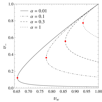
Figure 1: The fluid velocity behind the wall as a function of the wall velocity for the bag EOS (see below), for several values of $\alpha=L/(3w_{+})$.

The abovementioned divergence of $\partial v_{-}/\partial v_{w}|_{T_{+}}$ can be observed in the figure. It causes $v_{w}$ to be a minimum at the Jouguet point. As a consequence, for detonations the wall velocity is in the range $v_{J}\leq v_{w}<1$, where $v_{J}(T_{+})$ is velocity of the Jouguet detonation. It is well known that strong detonations are not compatible with the solutions for the fluid profile behind the wall. Therefore, the upper curves in Fig. 1 do not correspond to physical solutions. Weak detonations become weaker (i.e., $v_{-}$ decreases) for higher wall velocities. In the limit $v_{w}\to 1$, Eqs. (15) become

$$e_{-}-p_{-}=e_{+}-p_{+},\quad v_{-}=\frac{p_{-}-p_{+}}{e_{+}+p_{-}}=\frac{e_{-}-e_{+}}{e_{+}+p_{-}}.$$ (17)

The first of these equations gives the temperature $T_{-}$ as a function of $T_{+}$ for an ultra-relativistic stationary solution. The second one gives the fluid velocity behind the interface.

3.2 Runaway walls

If the wall is accelerated, we have to take into account the fact that a part of the energy accumulates in the wall [17]. In the time $\Delta t$, an amount of energy $A\Delta\sigma$ is accumulated in a surface area $A$ of the interface, where $\sigma$ is the surface energy density. Hence, the energy balance now gives

$$T_{-}^{0z}-T_{+}^{0z}=(T_{-}^{00}-T_{+}^{00})v_{w}+\frac{d\sigma}{dt}.$$ (18)

Similarly, since the momentum of a piece of wall is given by $A\sigma v_{w}$, we have

$$T_{-}^{zz}-T_{+}^{zz}=(T_{-}^{z0}-T_{+}^{z0})v_{w}+\frac{d(v_{w}\sigma)}{dt}.$$ (19)

After a certain (generally short) period of time, the accelerated wall will either reach a terminal velocity or accelerate to ultra-relativistic velocities. The ultra-relativistic accelerated regime is similar to the steady-state case in the sense that the wall velocity is essentially a constant, $v_{w}\simeq 1$ (although $\gamma_{w}$ and $\sigma$ vary). In this limit we have

$$\frac{d\sigma}{dt}=\frac{d(v_{w}\sigma)}{dt}=F_{\mathrm{net}},$$ (20)

where $F_{\mathrm{net}}$ is the net force per unit area acting on the wall. Inserting Eqs. (11-12) in (18-19) we obtain

$$e_{-}-p_{-}=e_{+}-p_{+}-2F_{\mathrm{net}},\quad v_{-}=\frac{w_{-}-w_{+}}{w_{-}+w_{+}}.$$ (21)

For $F_{\mathrm{net}}=0$, Eqs. (21) match the ultra-relativistic detonation case, Eq. (17). From Eqs. (21) we may obtain the temperature $T_{-}$ and the velocity $v_{-}$ as functions of $F_{\mathrm{net}}$ and $T_{+}$. We see that, for a constant net force, $v_{-}$ and $T_{-}$ are constant, like in the stationary case.

3.3 Fluid profiles

The profiles of $v$ and $T$ behind the wall are a solution of Eqs. (6) with boundary conditions $v=v_{-}$, $T=T_{-}$ at the wall. For a system with spherical, cylindrical or planar symmetry, the problem is 1+1 dimensional, since the fluid profile depends only on time and on the distance $r$ from the center, axis or plane of symmetry [22]. Besides, since there is no distance scale in the fluid equations, it is customary to assume the similarity condition, namely, that the solutions depend only on the variable $\xi=r/t$. With this assumption, one obtains the equation for the wall velocity [24]

$$\gamma^{2}(1-v\xi)\left[\frac{1}{c_{-}^{2}}\left(\frac{\xi-v}{1-\xi v}\right)^{2}-1\right]v^{\prime}=j\frac{v}{\xi},$$ (22)

where a prime indicates a derivative with respect to $\xi$, and $j=2$, $1$, or $0$ for spherical, cylindrical, or planar walls, respectively. The enthalpy profile is given by the equation

$$\frac{w^{\prime}}{w}=\left(\frac{1}{c_{-}^{2}}+1\right)\frac{\xi-v}{1-\xi v}\gamma^{2}v^{\prime}.$$ (23)

It is important to note that the similarity condition is compatible with a wall which is placed at a fixed value of $\xi$, namely, $\xi_{w}=v_{w}$. For an accelerated wall, this condition will not be compatible, in general, with the boundary conditions at the interface. Nevertheless, in the ultra-relativistic limit, the wall position corresponds essentially to the constant value $\xi_{w}=1$. Indeed, as we have seen, the values of $T_{-}$ and $v_{-}$ are constant in this limit for a constant $F_{\mathrm{net}}$. Therefore, the fluid profiles for the runaway solution can be obtained from Eqs. (22-23), like in the detonation case.

3.4 The bag EOS

In order to solve the hydrodynamic equations we need to consider a particular equation of state. We shall consider the bag EOS, in which the two phases consist of radiation and vacuum energy. This approximation has been widely used for simplicity, and also in order to obtain model-independent results which depend on a few physical quantities. Setting the vacuum energy in the low-temperature phase to zero, the model depends on three physical parameters, which we may choose to be the critical temperature $T_{c}$, the latent heat $L$, and the radiation constant of the high-temperature phase, $a$. Thus, we write

$$p_{+}(T)=\frac{1}{3}aT^{4}-\frac{L}{4},\quad p_{-}(T)=\frac{1}{3}\left(a-\frac{3L}{4T_{c}^{4}}\right)T^{4}.$$ (24)

The energy density of the high-temperature phase is of the form $e_{+}(T)=aT^{4}+\varepsilon$, where the false-vacuum energy density is given by $\varepsilon=L/4$. In the low-temperature phase, the energy density is of the form $e_{-}(T)=a_{-}T^{4}$, with a radiation constant given by $a_{-}=a(1-3\alpha_{c})$, where

$$\alpha_{c}=\varepsilon/(aT_{c}^{4}).$$ (25)

We define the usual bag variable

$$\alpha\equiv\varepsilon/(aT_{+}^{4})=L/(3{w_{+}}).$$ (26)

The enthalpy density is given by $w_{\pm}=(4/3)a_{\pm}T_{\pm}^{4}$ (with $a_{+}\equiv a$). For the bag EOS the speed of sound is the same in both phases, $c_{\pm}=1/\sqrt{3}$.

From Eqs. (15) we obtain the fluid variables behind a weak detonation wall,

$$v_{-} = \frac{3\alpha-1+3(1+\alpha)v_{w}^{2}-\sqrt{\left[3\alpha-1+3(1+\alpha)v_{w}^{2}\right]^{2}-12\alpha(2+3\alpha)v_{w}^{2}}}{2(2+3\alpha)v_{w}},$$ (27)

$$\frac{w_{-}}{w_{+}} = \frac{\gamma_{w}^{2}}{3}\left[1-3\alpha+3(1+\alpha)v_{w}^{2}-2\sqrt{\left(1-3\alpha+3(1+\alpha)v_{w}^{2}\right)^{2}-12v_{w}^{2}}\right]$$ (28)

(there is also a solution with a $+$ sign in front of the square roots, corresponding to strong detonations). Notice that the fluid velocity and the enthalpy ratio depend only on the variable $\alpha$ and the wall velocity. On the other hand, the temperature is given by

$$\frac{T_{-}^{4}}{T_{+}^{4}}=\frac{1}{1-3\alpha_{c}}\,\frac{w_{-}}{w_{+}}.$$ (29)

The Jouguet velocity is obtained by considering the condition (16) together with Eqs. (15). For the bag EOS we obtain

$$v_{J}=\frac{\sqrt{2\alpha+3\alpha^{2}}+1}{\sqrt{3}(1+\alpha)}.$$ (30)

The ultra-relativistic limit can be obtained either by taking the limit $v_{w}\rightarrow 1$ in Eqs. (27-28), or directly from (17). We have

$$\frac{w_{-}}{w_{+}}=1+3\alpha,\quad v_{-}=\frac{3\alpha}{2+3\alpha}\quad\mbox{(UR detonation).}$$ (31)

For a runaway wall we obtain, from Eqs. (21),

$$\frac{w_{-}}{w_{+}}=1+3(\alpha-\bar{F}),\quad v_{-}=\frac{3(\alpha-\bar{F})}{2+3(\alpha-\bar{F})}\quad\mbox{(runaway)},$$ (32)

where

$$\bar{F}\equiv\frac{F_{\mathrm{net}}}{aT_{+}^{4}}=\frac{4}{3}\frac{F_{\mathrm{net}}}{w_{+}}.$$ (33)

Notice that Eqs. (32) match the detonation case for $F_{\mathrm{net}}=0$. On the other hand, as $F_{\mathrm{net}}$ increases, $T_{-}$ and $v_{-}$ decrease. Hence, the hydrodynamics becomes weaker for larger acceleration. This behavior is similar to the detonation case, in which the higher the wall velocity, the weaker the hydrodynamics (see Fig. 2). This is related to the fact that the hydrodynamics obstructs the wall motion [11, 12]. Moreover, we see that for $\bar{F}=\alpha$ we have $w_{-}=w_{+}$ and $v_{-}=0$, i.e., the fluid remains unperturbed after the passage of the wall.

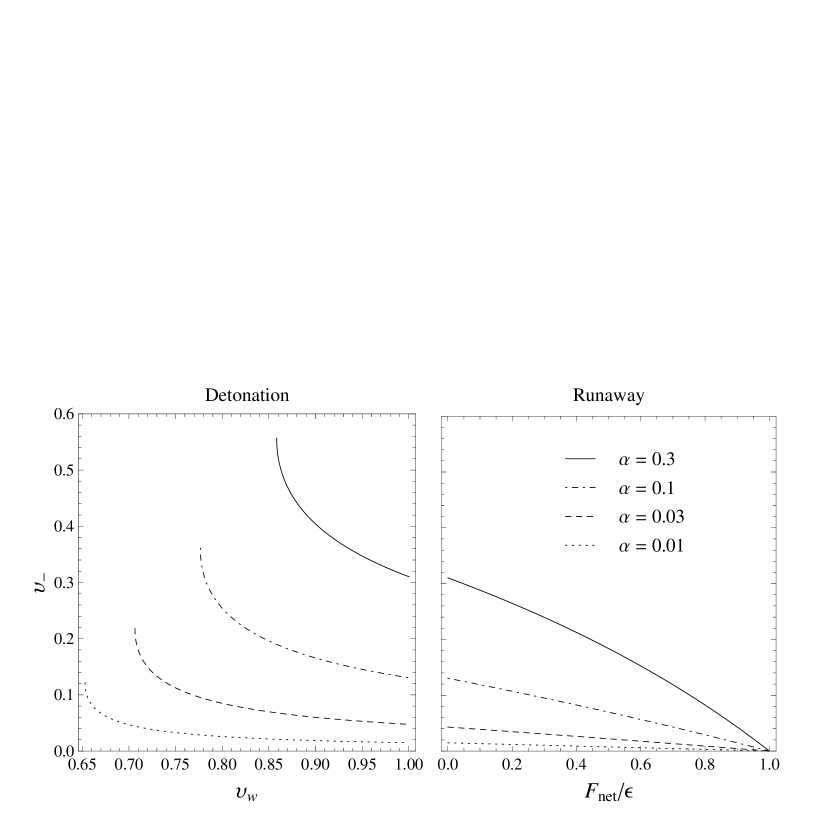
Figure 2: The fluid velocity behind the wall as a function of the wall velocity for the case of a detonation (left panel) and as a function of the net force for the case of a runaway wall (right panel).

The condition $\bar{F}=\alpha$ sets a maximum value for the net force, which is given by the false vacuum energy density, $F_{\mathrm{\max}}=\varepsilon$. To understand this physically, notice that the force which drives the wall motion is essentially given by the pressure difference between the two phases. This force vanishes at the critical temperature and reaches its maximum at zero temperature. At $T=0$ the pressure difference is just given by the zero-temperature effective potential, and coincides with the false-vacuum energy density. In the bag model, this is given by the parameter $\varepsilon$ (at finite temperature there is also a friction force due to the plasma, but at zero temperature the friction force vanishes). Therefore, $F_{\mathrm{net}}$ can reach the maximum value $\varepsilon$ if the phase transition occurs at $T_{+}=0$. However, such an extreme supercooling is not likely in concrete physical models.

For the bag EOS it is relatively simple to obtain the fluid profiles, since $c_{-}$ is a constant. However, except for the planar case, the fluid equations (22-23) must be solved numerically. Behind the wall, the solutions which fulfil the boundary condition of a vanishing fluid velocity at $\xi=0$ are rarefaction waves, in which $v(\xi)$ actually vanishes for $0<\xi<c_{-}$ and grows for $\xi>c_{-}$ up to the boundary value $v_{-}$ at $\xi=\xi_{w}$ (see e.g. [20, 24]). The temperature and pressure also decrease away from the wall. These can be computed from the enthalpy profile, which is readily obtained by integrating Eq. (23),

$$\frac{w}{w_{-}}=\exp\left[\left(\frac{1}{c_{-}^{2}}+1\right)\int_{v_{-}}^{v}\frac{\xi-v}{1-\xi v}\gamma^{2}\,dv\right].$$ (34)

In Fig. 3 we show some profiles for the case of spherically-symmetric bubbles.

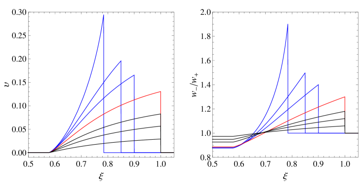
Figure 3: Fluid velocity and enthalpy profiles for spherical bubbles, for $\alpha=0.1$ and different wall velocities. The highest curve corresponds to a Jouguet detonation with wall velocity $v_{J}(\alpha)\simeq 0.78$. The other blue curves correspond to weak detonations with velocities $v_{w}=0.85$ and $v_{w}=0.92$. The red curve corresponds to the limit of a detonation with $v_{w}\rightarrow 1$ or a runaway wall with $F_{\mathrm{net}}\rightarrow 0$. The black curves correspond to runaway walls with $F_{\mathrm{net}}/F_{\max}=0.4$, $0.6$, and $0.8$.

3.5 Efficiency factors

For the bag EOS, the efficiency factor is defined as the fraction of the released vacuum energy $\varepsilon$ which goes into bulk motions of the fluid,

$$\kappa_{\mathrm{fl}}\equiv\frac{E_{\mathrm{kin}}}{\varepsilon V_{b}},$$ (35)

where $V_{b}$ is the volume of the bubble. We have, for the different wall symmetries [24],

$$\kappa_{\mathrm{fl}}=\frac{j+1}{\varepsilon v_{w}^{j+1}}\int_{0}^{\infty}\!d\xi\,\xi^{j}\,w\,\gamma^{2}v^{2}.$$ (36)

As can be seen from Eq. (34), for detonations or runaway walls the profile of $w/w_{-}$ does not depend on $w_{-}$ but only on the profile of $v$, which only depends on the boundary values $v_{w},v_{-}$. As a consequence, we can write

$$\kappa_{\mathrm{fl}}=\frac{j+1}{v_{w}^{j+1}}\,\frac{4}{3\alpha}\frac{w_{-}}{w_{+}}\,I(v_{w},v_{-}),$$ (37)

with

$$I(v_{w},v_{-})=\int_{c_{-}}^{v_{w}}\!d\xi\,\xi^{j}\,\frac{w}{w_{-}}\,\gamma^{2}v^{2}.$$ (38)

For detonations, $v_{-}$ and $w_{-}/w_{+}$ are functions of $\alpha$ and $v_{w}$, and therefore the efficiency factor depends only on these quantities, $\kappa_{\mathrm{fl}}=\kappa_{\mathrm{fl}}^{\mathrm{det}}(\alpha,v_{w})$. On the other hand, for runaway walls we have $v_{w}=1$, while $w_{-}/w_{+}$ and $v_{-}$ depend on $\alpha$ and $\bar{F}$. From Eqs. (37) and (32), in this case $\kappa_{\mathrm{fl}}$ is of the form

$$\kappa_{\mathrm{fl}}^{\mathrm{run}}(\alpha,\bar{F})=\frac{j+1}{3}\,\frac{4(1+3\alpha-3\bar{F})}{\alpha}\,I_{1}(v_{-}),$$ (39)

where $I_{1}(v_{-})=I(1,v_{-})$.

For the planar case the integral (38) can be done analytically [24], while for spherical or cylindrical walls it must be calculated numerically. Notice that $w_{-}$ and $v_{-}$ are the same for all these cases, but the rarefaction profiles differ. In Fig. 4 we show the value of the efficiency factor for spherical and planar walls. The cylindrical case lies between the other two. For steady-state walls we plotted $\kappa_{\mathrm{fl}}$ as a function of the wall velocity (left panel), while for runaway walls we plotted it as a function of the net force (right panel).

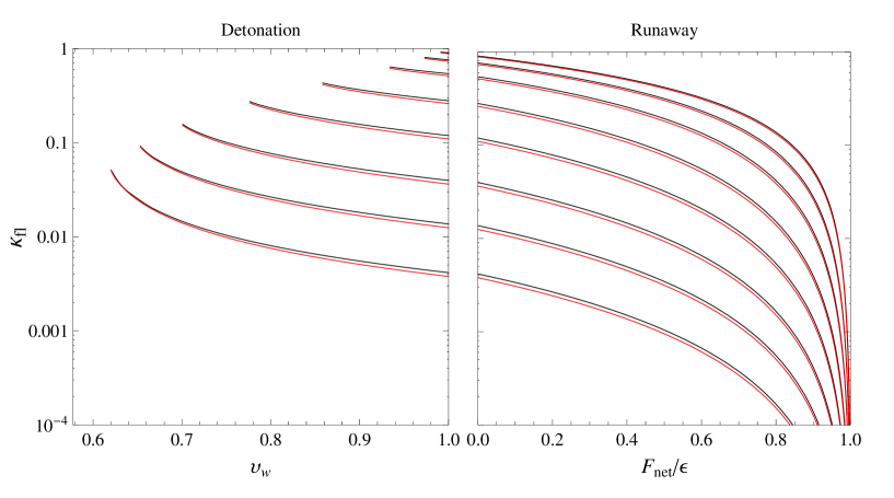
Figure 4: The efficiency factor for spherical (black) and planar (red) walls, for several values of $\alpha$. From bottom to top, $\alpha=0.003,0.01,0.03,0.1,0.3,1,3,10$.

For the range of values shown in the figure, the difference between the two wall symmetries is always less than a 10%, while this relative difference is exceeded only for $F_{\mathrm{net}}$ very close to $F_{\max}=\varepsilon$, where $\kappa_{\mathrm{fl}}\rightarrow 0$. As already discussed, it is not likely that such values of $F_{\mathrm{net}}$ will be reached in a physical model. Such a small difference is interesting, since for planar walls we obtain analytic results (see the appendix). In the appendix we also give fits for spherical detonations and runaway walls, where the relative error is smaller than a 3% in the whole detonation range and in most of the runaway range.

For comparison, we show in Fig. 5 the value of $\kappa_{\mathrm{fl}}$ in the different regimes, for some values of the bag parameter $\alpha$ (for the calculation in the cases of weak and Jouguet deflagrations, see [24]). The different types of stationary solutions are divided by the points $v_{w}=c_{-}$ and $v_{w}=v_{J}(\alpha)$.

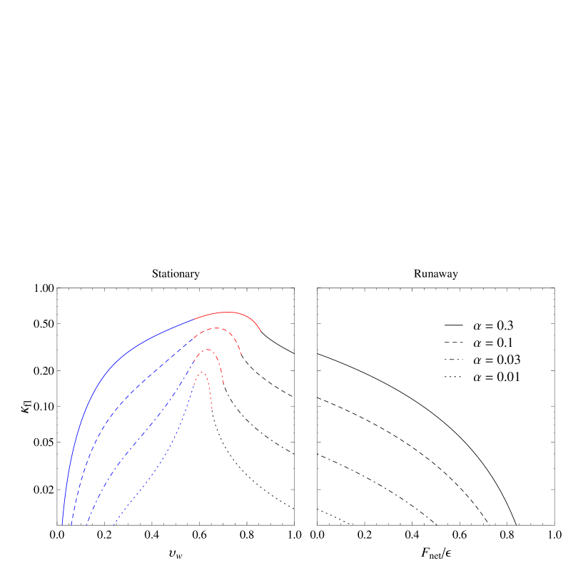
Figure 5: The efficiency factor $\kappa_{\mathrm{fl}}$ for spherical bubbles. Blue curves correspond to weak deflagrations, red curves to Jouguet deflagrations, and black curves to weak detonations or runaway walls.

As already discussed, the hydrodynamics of weak detonations becomes weaker as the wall velocity increases, and it becomes even weaker for runaway walls. This is reflected in the efficiency factor, which is monotonically decreasing in these regimes. On the other hand, for small wall velocities (i.e., for weak deflagrations) the efficiency factor increases with the wall velocity, and is maximal for supersonic (Jouguet) deflagrations.

In the runaway case, a portion of the released vacuum energy goes into kinetic energy of the wall. This will increase the efficiency for gravitational wave generation through direct bubble collisions. This fraction is given by

$$\kappa_{\mathrm{wall}}\equiv\frac{\Delta E_{\mathrm{wall}}}{\varepsilon\Delta V_{b}}.$$ (40)

Considering a small piece of the thin interface, the energy which goes to the corresponding volume $\Delta V_{b}=Av_{w}\Delta t$ is given by $\Delta E_{\mathrm{wall}}=\Delta\sigma A$. Therefore, we have, from Eq. (20) and the definitions (26,33),

$$\kappa_{\mathrm{wall}}=\frac{d\sigma/dt}{\varepsilon v_{w}}=\frac{F_{\mathrm{net}}}{\varepsilon}=\frac{\bar{F}}{\alpha}.$$ (41)

4 The wall equation of motion

We shall now consider the equation of motion for the wall. At a given point of the thin interface we may place the $z$ axis perpendicular to the wall. Then the field equation (5) with the damping (8) becomes

$$(\partial_{0}^{2}-\partial_{z}^{2})\phi+\partial\mathcal{F}/\partial\phi+\mathcal{K}=0.$$ (42)

If we describe the wall at rest by a certain field profile $\phi_{0}(z)$ which varies between the values $\phi_{-}$ and $\phi_{+}$, then, in the plasma frame, we have

$$\phi(z,t)=\phi_{0}(\gamma_{w}\left(z-z_{w}\right)),$$ (43)

where $z_{w}$ depends on time and we have $v_{w}=\dot{z}_{w}$, $\gamma_{w}=1/\sqrt{1-v_{w}^{2}}$. The wall corresponds to the range of $z$ where $\phi$ varies, and we define the wall position $z_{w}(t)$ by the condition $\int(\partial_{z}\phi)^{2}(z-z_{w})\,dz\,=0$. Multiplying Eq. (42) by $\partial_{z}\phi$ and integrating across the wall, we obtain the equation

$$\sigma_{0}\gamma_{w}^{3}\dot{v}_{w}=\int_{-}^{+}\frac{\partial\mathcal{F}}{\partial\phi}\,\frac{\partial\phi}{\partial z}\,dz+\int_{-}^{+}\mathcal{K}\,\frac{\partial\phi}{\partial z}\,dz,$$ (44)

where $\int_{-}^{+}dz$ means integration between points on each side of the wall (where $\partial_{z}\phi$ vanishes) and

$$\sigma_{0}=\int_{-}^{+}\left[\phi_{0}^{\prime}(z)\right]^{2}dz.$$ (45)

This integral gives the surface energy density of the wall at rest. We see that it appears in the left-hand side of Eq. (44) multiplying the proper acceleration $\gamma_{w}^{3}\dot{v}_{w}$. Hence, the terms in the right-hand side are forces (per unit area) acting on the wall. Since the force which drives the wall motion is finite, the factor $\gamma_{w}^{3}$ implies that, in the plasma frame, $\dot{v}_{w}$ decreases as the wall approaches the speed of light.

The force terms in Eq. (44) depend not only on the Higgs profile but also on the fluid profiles. The first of them is very sensitive to hydrodynamics. For a constant temperature, this term gives the pressure difference $p_{-}-p_{+}$. Since it is always positive, we shall refer to it as the driving force $F_{\mathrm{dr}}$. The term containing $\mathcal{K}$ represents the microscopic departures from equilibrium caused by the moving wall. It is always negative and velocity dependent. We shall refer to this term as the friction force $F_{\mathrm{fr}}$. Thus, Eq. (44) can be written as

$$F_{\mathrm{net}}=F_{\mathrm{dr}}+F_{\mathrm{fr}}.$$ (46)

4.1 Driving force and hydrodynamic obstruction

The driving force can be written in the form [14]

$$F_{\mathrm{dr}}=p_{-}-p_{+}-\int_{-}^{+}\frac{\partial\mathcal{F}}{\partial T^{2}}\,{dT^{2}},$$ (47)

which we shall approximate for definite calculations by

$$F_{\mathrm{dr}}\simeq p_{-}-p_{+}-\left\langle\frac{\partial\mathcal{F}}{\partial T^{2}}\right\rangle(T_{+}^{2}-T_{-}^{2}),$$ (48)

where we have approximated the value of ${\partial\mathcal{F}}/{\partial T^{2}}$ inside the wall by

$$\left\langle\frac{\partial\mathcal{F}}{\partial T^{2}}\right\rangle\equiv\frac{1}{2}\left(\frac{\partial\mathcal{F_{+}}}{\partial T_{+}^{2}}+\frac{\partial\mathcal{F_{-}}}{\partial T_{-}^{2}}\right).$$ (49)

For the bag EOS, Eq. (48) takes the simple form

$$F_{\mathrm{dr}}=\frac{L}{4}\left(1-\frac{T_{-}^{2}T_{+}^{2}}{T_{c}^{4}}\right)=\varepsilon-\varepsilon\frac{T_{-}^{2}T_{+}^{2}}{T_{c}^{4}}.$$ (50)

In this approximation, the first term is the zero-temperature part of the force. Indeed, as already mentioned, the false vacuum energy density is given by the zero-temperature effective potential. Thus, for a physical model the bag constant $\varepsilon$ would be given by $V(\phi_{+})-V(\phi_{-})$. The second term in Eq. (50) is the temperature-dependent part of the driving force, and contains the effect of hydrodynamics. For weak detonations, this effect is to increase $T_{-}$ with respect to the outside temperature $T_{+}$, and hence to decrease the driving force. In this decomposition, the term $F_{\mathrm{hyd}}=-(L/4){T_{-}^{2}T_{+}^{2}}/{T_{c}^{4}}$ can be seen as a force which opposes the wall motion and depends indirectly on the wall velocity (through the dependence of the temperature on $v_{w}$). However, this hydrodynamic obstruction does not behave as a fluid friction, since it decreases with the wall velocity. Indeed, the reheating behind the wall is highest for $v_{w}$ close to the Jouguet point and lowest for $v_{w}\rightarrow 1$. It is worth remarking that the approximation (50) preserves this important effect of reheating, while simpler approximations such as setting $T_{-}=T_{+}$ in Eq. (47) (see e.g. [20]) overestimate the driving force.

4.2 Friction force

As already discussed, the friction must be obtained from microphysics considerations which are much more involved than the calculation of $F_{\mathrm{dr}}$. Here we shall use instead the phenomenological damping (8). Hence, we have

$$F_{\mathrm{fr}}=\int_{-}^{+}\frac{f(\phi)\,u^{\mu}\partial_{\mu}\phi}{\sqrt{1+[g(\phi)\,u^{\mu}\partial_{\mu}\phi]^{2}}}\,\partial_{z}\phi\,dz.$$ (51)

For the field profile (43), we have

$$u^{\mu}\partial_{\mu}\phi=\gamma(\partial_{0}\phi+v\partial_{z}\phi)=\phi_{0}^{\prime}\gamma[\gamma_{w}(v-v_{w})+\dot{\gamma}_{w}(z-z_{w})].$$ (52)

The term $\dot{\gamma}_{w}(z-z_{w})$ vanishes in the stationary case. In the runaway regime we can also neglect it, since $\phi_{0}^{\prime}$ vanishes out of the thin interface. We thus have

$$F_{\mathrm{fr}}=\int_{-}^{+}\frac{\gamma_{w}\gamma(v-v_{w})f(\phi_{0})(\phi_{0}^{\prime})^{2}}{\sqrt{1+\gamma_{w}^{2}\gamma^{2}(v-v_{w})^{2}g^{2}(\phi_{0})(\phi_{0}^{\prime})^{2}}}\,dz,$$ (53)

where we have used the change of variable of integration $\gamma_{w}(z-z_{w})\to z$. It is easy to see that in the limit $\gamma_{w}\to\infty$ we have $F_{\mathrm{fr}}\sim$ constant, while for $v_{w}\ll 1$ (which implies $v\ll 1$ as well) we have $F_{\mathrm{fr}}\sim v_{w}$. The result (53) is equivalent to that of Ref. [21], as can be seen from the transformation $\gamma v\to\gamma\gamma_{w}(v-v_{w})$ from the wall frame to the plasma frame.

The integral in Eq. (53) is of the form $\int[\phi_{0}^{\prime}(z)]^{2}F(z)\,dz$, where the function $[\phi_{0}^{\prime}(z)]^{2}$ vanishes outside the wall and peaks at the center of the latter. Therefore, we can write this integral as $F(\bar{z})\int[\phi_{0}^{\prime}(z)]^{2}dz=F(\bar{z})\sigma_{0}$, where $\bar{z}$ is some point near the wall center. We thus obtain

$$F_{\mathrm{fr}}=\frac{\eta\gamma_{w}\bar{\gamma}(\bar{v}-v_{w})}{\sqrt{1+\lambda^{2}\gamma_{w}^{2}\bar{\gamma}^{2}(\bar{v}-v_{w})^{2}}},$$ (54)

where $\bar{\gamma},\bar{v}$ are the values of $\gamma,v$ at the center of the wall, $\eta=\sigma_{0}f(\phi_{0}(\bar{z}))$, and $\lambda$ is similarly given by the function $g$ and details of the wall profile. We shall regard $\eta$ and $\lambda$ as free parameters which can be chosen appropriately to give the correct numerical values of the friction in the NR and UR limits. On the other hand, we shall approximate the value of $\bar{v}$ by the average

$$\bar{v}=({v_{-}+v_{+}})/{2}=v_{-}/2,$$ (55)

and $\bar{\gamma}=1/\sqrt{1-\bar{v}^{2}}$.

For non-relativistic velocities, Eq. (54) gives a friction force which is proportional to the relative velocity, $F_{\mathrm{fr}}=-\eta\,(v_{w}-\bar{v})$, as expected. For a specific model, the value of $\eta$ can be obtained by comparison with the result of a non-relativistic microphysics calculation. Therefore, we use the notation $\eta=\eta_{NR}$. It is out of the scope of the present work to compute the friction for specific models. General approximations for $\eta_{NR}$ as a function of the parameters for a variety of models can be found in Ref. [27]. The friction coefficient depends on temperature. In particular, it decreases as $T$ decreases, since the friction depends on the particle populations. Nevertheless, in contrast to $F_{\mathrm{dr}}$, the friction is not sensitive to the temperature difference $T_{c}-T$. Therefore, it is not very sensitive to hydrodynamics. For specific calculations, in this work we shall assume that, roughly, $\eta_{NR}\sim T_{+}^{4}$.

In the ultra-relativistic case $\gamma_{w}\gg 1$, Eq. (54) gives $F_{\mathrm{fr}}=-\eta/\lambda$. Therefore, we define the UR friction coefficient $\eta_{UR}=-\eta/\lambda$, so that $F_{\mathrm{fr}}=-\eta_{UR}v_{w}$. The value of this parameter for a specific model can be obtained from the microphysics result (7). This result, however, gives the total UR force $F_{\mathrm{net}}$ rather than the friction. Notice that the last term in Eq. (7) includes the finite-temperature part of the driving force, $F_{\mathrm{hyd}}$, as well as the friction. We may obtain the UR friction force as $F_{\mathrm{fr}}=F_{\mathrm{net}}-F_{\mathrm{dr}}$, taking into account the UR limit of the driving force. The latter is given by Eqs. (50), (29), and (32). We obtain

$$\frac{\eta_{UR}}{aT_{+}^{4}}=\alpha-\bar{F}-\alpha_{c}\sqrt{\frac{1+3(\alpha-\bar{F})}{1-3\alpha_{c}}}.$$ (56)

For a given model, the quantities $\alpha=L/(3w_{+})$ and $\bar{F}=4F_{\mathrm{net}}/(3w_{+})$ can be obtained as functions of the nucleation temperature $T_{+}$. We remark that, although decomposing the total force into driving and friction forces is not relevant for the runaway regime, determining the UR value of the friction component is relevant for a correct use of Eq. (54) as an interpolation between the NR and UR cases. In terms of the friction coefficients $\eta_{NR},\eta_{UR}$, we have

$$F_{\mathrm{fr}}=-\frac{\eta_{NR}\eta_{UR}\,\gamma_{w}\bar{\gamma}(v_{w}-\bar{v})}{\sqrt{\eta_{UR}^{2}+\eta_{NR}^{2}\,\gamma_{w}^{2}\bar{\gamma}^{2}(v_{w}-\bar{v})^{2}}}.$$ (57)

It is worth commenting on previous approaches. A similar, but simpler, phenomenological model for the friction was considered in Ref. [20]. The approximation involves a single free parameter and is equivalent to setting $\lambda=1$ in Eq. (54). Although this model gives a friction which saturates at high $\gamma_{w}$, it is numerically incorrect as it corresponds to the case $\eta_{UR}=\eta_{NR}$ (besides, the approximation $T_{-}=T_{+}$ was used in [20] for the driving force; we shall discuss on this approximation below). The phenomenological model (8) was already considered in Ref. [21]. The resulting friction is equivalent to Eq. (54). However, in [21] the hydrodynamics was neglected for runaway walls (but not for stationary solutions). That is, the relation $T_{-}=T_{+}$ was assumed for the runaway case. This results in a different value of $\eta_{UR}$, as the right-hand side of Eq. (56) becomes $\alpha-\bar{F}-\alpha_{c}$. Since, on the other hand, the hydrodynamics was taken into account for detonations, the stationary solutions did not match continuously the accelerated ones. This is not correct since, as we have seen, the hydrodynamics of a runaway wall is similar to that of the detonation, and matches the latter for $F_{\mathrm{net}}=0$.

4.3 The wall velocity

From Eqs. (46), (50) and (57), we have, for detonations or runaway walls,

$$\frac{F_{\mathrm{net}}}{aT_{+}^{4}}=\alpha-\alpha_{c}\frac{T_{-}^{2}}{T_{+}^{2}}-\frac{\bar{\eta}_{NR}\bar{\eta}_{UR}\,(v_{w}-\bar{v}_{-})}{\sqrt{\bar{\eta}_{UR}^{2}(1-v_{w}^{2})(1-\bar{v}_{-}^{2})+\bar{\eta}_{NR}^{2}\,(v_{w}-\bar{v}_{-})^{2}}}$$ (58)

where $\bar{v}=v_{-}/2$, and we use the notation $\bar{\eta}=\eta/(aT_{+}^{4})$ for the two friction coefficients. In the UR limit, Eq. (58) becomes

$$\bar{F}=\alpha-{\alpha_{c}}{T_{-}^{2}}/{T_{+}^{2}}-\bar{\eta}_{UR}.$$ (59)

We remark again that the latter equation is just a decomposition of the UR net force, which actually defines the value of the friction coefficient $\eta_{UR}$, while the former gives an equation of motion for the wall away from that limit. In particular, if the microphysics computation of the net force, Eq. (7), gives $F_{\mathrm{net}}<0$, it means that, in fact, the wall will never reach the UR regime. Nevertheless, the UR calculation is still useful and Eq. (59) makes sense. The interpretation is that the UR friction is so high that the driving force cannot compensate it. In this case we just obtain $\bar{\eta}_{UR}$ from Eq. (56), and then compute the steady-state wall velocity by setting $F_{\mathrm{net}}=0$ in Eq. (58).

To solve for $v_{w}$, we must use Eqs. (27-29) for $v_{-}$ and $T_{-}$. It is worth mentioning that, for detonations, the result does not depend on the wall being spherical or planar, since all the quantities appearing in Eq. (58) are the same in the two cases. This is because the relations between $v_{-},T_{-}$ and $v_{+},T_{+}$ are the same for spherical or planar walls. Besides, for detonations the conditions in front of the wall (i.e., $v_{+},T_{+}$) are also the same (in contrast, for deflagrations, the fluid in front of the wall is perturbed differently for planar or spherical walls).

We show the result in Fig. 6 (solid line) for fixed values of the friction parameters and varying the bag quantity $\alpha$. For concreteness, and in order to compare with previous results, we consider the case $\eta_{UR}=\eta_{NR}$ (for other cases and different parameter variations, see [21]). The vertical dashed lines delimit the weak detonation solutions. Increasing $\alpha$ generally increases the driving force and, consequently, the wall velocity. The figure does not show the deflagration cases, for which $v_{w}\lesssim c_{-}$ (there is a discontinuity between deflagrations and detonations).

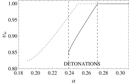
Figure 6: The wall velocity for $\alpha_{c}=0.05$, $\bar{\eta}_{UR}=0.2$, and $\eta_{NR}=\eta_{UR}$. The dotted line corresponds to the approximation $T_{-}=T_{+}$.

The dotted line in Fig. 6 is obtained by neglecting the reheating in the calculation of the driving force, i.e., setting $T_{-}=T_{+}$, for which the driving-force term in Eq. (58) becomes $\alpha-\alpha_{c}$. This was used as an approximation in Ref. [20]. We consider it here in order to appreciate the role of hydrodynamics. Quantitatively, we see that this approximation overestimates the driving force, as we obtain higher values of the velocity. Besides, we observe a significant qualitative difference between the two results at the lower end of the detonation curve. This end corresponds to the Jouguet point. Since the hydrodynamics becomes very strong near this point, Eq. (58) gives two solutions for $v_{w}$, while the approximation $T_{-}=T_{+}$ completely misses this effect. In Ref. [14] it was shown that weak detonations corresponding to the lower branch of solutions are unstable.

The value of $\alpha$ for which the detonation reaches the ultra-relativistic regime in Fig. 6 can be obtained from Eq. (59) which, for $\bar{F}=0$, gives $\alpha={\alpha_{c}}{T_{-}^{2}}/{T_{+}^{2}}+{\bar{\eta}_{UR}}$. Notice that $T_{-}$ actually depends on $\alpha$ through Eqs. (29,31), ${T_{-}^{4}}/{T_{+}^{4}}=({1+3\alpha})/({1-3\alpha_{c}})$. Thus, for given values of $\alpha_{c}$ and $\bar{\eta}_{UR}$ we have a quadratic equation for $\alpha$ (or for $T_{-}$), which yields

$$\alpha=\alpha_{c}\,{T_{0}^{2}}/{T_{+}^{2}}+{\bar{\eta}_{UR}}\equiv\alpha_{0},$$ (60)

where $T_{0}$ is the corresponding value of $T_{-}$, given by

$$\frac{T_{0}^{4}}{T_{+}^{4}}=\frac{3\alpha_{c}}{2(1-3\alpha_{c})}\left[1+\sqrt{1+\frac{4(1+3\bar{\eta}_{UR})(1-3\alpha_{c})}{3\alpha_{c}^{2}}}\right].$$ (61)

For $\alpha>\alpha_{0}$, the steady-state equation gives $v_{w}>1$, which actually indicates that the friction force cannot compensate the driving force and we have $F_{\mathrm{net}}>0$, i.e., a runaway wall.

In the runaway regime, we have a proper acceleration which is proportional to the net force. It is interesting to calculate the value of $F_{\mathrm{net}}$ corresponding to Fig. 6, which can be obtained from Eq. (59) [although for a given model one would rather compute $F_{\mathrm{net}}$ directly from Eq. (7), and then determine $\eta_{UR}$]. We must take into account the dependence of $T_{-}$ on $F_{\mathrm{net}}$, which is given by Eqs. (29,32),

$$T_{-}^{4}/T_{+}^{4}=(1+3\alpha-3\bar{F})/(1-3\alpha_{c}).$$ (62)

From Eqs. (62) and (59) we obtain quadratic equations for $\bar{F}$ and $T_{-}/T_{+}$ as functions of $\alpha$, $\alpha_{c}$, and $\bar{\eta}_{UR}$. Nevertheless, the dependence on $\alpha$ cancels in the equation for $T_{-}$, and we obtain

$$T_{-}=T_{0},\quad\bar{F}=\alpha-\alpha_{c}T_{0}^{2}/T_{+}^{2}-\bar{\eta}_{UR}=\alpha-\alpha_{0},$$ (63)

with $\alpha_{0}$ and $T_{0}$ given by Eqs. (60-61). On the other hand, if we use the approximation $T_{-}=T_{+}$, we just neglect Eq. (62), while Eq. (59) gives $\bar{F}=\alpha-\alpha_{c}-\bar{\eta}_{UR}$. This result can also be written in the form $\bar{F}=\alpha-\alpha_{0}$, but the value of $\alpha_{0}$ is different, namely, $\alpha_{0}=\alpha_{c}+\bar{\eta}_{UR}$. In Fig. 7 we plot the net force, normalized to its maximum value $\varepsilon$, as a function of $\alpha$ for the parameters of Fig. 6. We see that neglecting the hydrodynamics gives a higher wall acceleration.

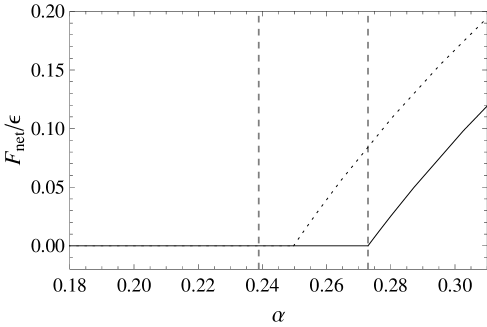
Figure 7: The net force corresponding to Fig. 6.

Comparing the solid lines of Figs. 6 and 7, we see that the detonation solution matches the runaway solution at $\alpha=\alpha_{0}$. In Ref. [21] this matching does not occur, due to the assumption of different hydrodynamics. As a consequence, the two kinds of solutions were found to coexist in a small parameter range. We do not find such a coexistence of detonation and runaway solutions here, since the hydrodynamics is continuous with $v_{w}$ and $\bar{F}$. In fact, coexistence of solutions could arise also due to strong hydrodynamics, even if the hydrodynamics varies continuously with the parameters. For instance, we have multiple weak-detonation solutions near the Jouguet point, even though $v_{-},T_{-}$ are continuous functions of $\alpha,v_{w}$. This does not happen in the UR limit, since the perturbations of the fluid vary continuously with $\alpha,v_{w}$, and $\bar{F}$ and, besides, the hydrodynamics is weaker.

4.4 Microphysics and released energy

In Sec. 3 we computed the fractions of the released vacuum energy which go into bulk motions of the fluid and into kinetic energy of the bubble wall, as functions of the quantities $v_{w}$, $\bar{F}=(4/3)F_{\mathrm{net}}/w_{+}$, and $\alpha=L/(3w_{+})$. For a given model, the nucleation temperature and the thermodynamical quantities $L,w_{+}$ can be calculated from the finite-temperature effective potential (1), and the net force can be readily computed from Eq. (7). This gives the values of $\alpha$ and $\bar{F}$. The steady-state wall velocity can be obtained from Eq. (58), after determining the friction coefficients $\eta_{UR}$ and $\eta_{NR}$. The value of $\eta_{UR}$ can be obtained from $\bar{F}$ using Eq. (56), while $\eta_{NR}$ must be obtained from a microphysics calculation. Such a computation is beyond the scope of this paper. Here, we shall only consider the energy distribution among the fluid and the wall for the parameter variation of Figs. 6 and 7. As already discussed, this parameter variation becomes rather artificial in the runaway regime. It is useful, though, for a comparison with previous results.

The fraction of energy accumulated in the interface, $\kappa_{\mathrm{wall}}$, is just given by $F_{\mathrm{net}}/\varepsilon$, which is plotted in Fig. 7. In Fig. 8 we consider a wider range of runaway solutions, and we plot separately (in the right panel) the result obtained by using the approximation $T_{-}=T_{+}$ in the calculation of the driving force. The value of $\kappa_{\mathrm{wall}}$ is represented by the height of the light shade. Thus, the curves delimiting this region in the left and right panels of Fig. 8 correspond, respectively, to the solid and dotted lines of Fig. 7. Following Ref. [20], we plot the value of $\kappa_{\mathrm{fl}}$ (for spherical bubbles) added to that of $\kappa_{\mathrm{wall}}$. This gives the upper curves delimiting the dark shade regions. Hence, the fraction of $\varepsilon$ which goes into bulk fluid motions is represented by the dark shade. Accordingly, the white region indicates the portion of $\varepsilon$ which goes into reheating. The vertical line separates the detonation and runaway regimes. We include the complete detonation range (which is different in the two panels).

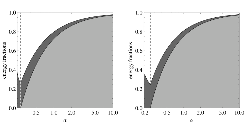
Figure 8: The fractions of vacuum energy which go to the wall and the fluid, for the same case of Figs. 6 and 7. The right panel corresponds to neglecting the reheating in the calculation of the driving force.

The right panel of Fig. 8 agrees with the results of Ref. [20]. The values of the parameters, namely, $\eta_{NR}=\eta_{UR}=0.2$, $a_{-}/a_{+}=1-3\alpha_{c}=0.85$, correspond to one of the cases considered in that work (cf. the left panel of Fig. 12 in [20]). We observe that the two panels of Fig. 8 are qualitatively similar, particularly for the runaway regime, where the hydrodynamics is weaker. The difference is more apparent for detonations, where the hydrodynamics is strongest. In fact, the Jouguet point is never reached in the left panel. The quantitative difference between the two calculations is better appreciated in Figs. 6 and 7. For a given $\alpha$, neglecting the hydrodynamics gives higher wall velocities and accelerations and, hence, a larger $\kappa_{\mathrm{wall}}$ and a smaller $\kappa_{\mathrm{fl}}$. It is worth emphasizing that in both panels we have used the results from Sec. 3 in terms of $\alpha$, $v_{w}$ and $\bar{F}$, and the discrepancy originates in the computation of $v_{w}$ and $\bar{F}$.

For the runaway case we may obtain simple semi-analytical expressions for the efficiency factors as functions of the quantities $\alpha$, $\alpha_{c}$, and $\bar{\eta}_{UR}$. From Eqs. (41) and (63), we have

$$\kappa_{\mathrm{wall}}=1-{\alpha_{0}}/{\alpha}.$$ (64)

This is valid for the two plots of Fig. 8, with different values of $\alpha_{0}(\alpha_{c},\bar{\eta}_{UR})$. Since $\kappa_{\mathrm{wall}}$ gives the fraction of $\varepsilon$ which goes to kinetic energy of the wall, Eq. (64) indicates that a fraction $\alpha_{0}/\alpha$ goes to the fluid (either to bulk motions or reheating). Moreover, using Eq. (63) in Eqs. (39) and (32), we have

$$\kappa_{\mathrm{fl}}^{\mathrm{run}}=\frac{4(1+3\alpha_{0})I_{1}(v_{-})}{\alpha},\quad\mbox{with}\quad v_{-}=\frac{3\alpha_{0}}{2+3\alpha_{0}}.$$ (65)

Hence, the runaway efficiency factor can be written as

$$\kappa_{\mathrm{fl}}^{\mathrm{run}}=\kappa_{UR}^{\mathrm{det}}\,{\alpha_{0}}/{\alpha},$$ (66)

where $\kappa_{UR}^{\mathrm{det}}\equiv\kappa_{\mathrm{fl}}^{\mathrm{det}}(\alpha_{0},v_{w}=1)$ is the efficiency factor of the UR detonation. The functional dependence of Eqs. (64) and (66) on $\alpha$ agrees with the results of Ref. [20]. The quantitative difference, which is illustrated by the two panels of Fig. 8, is due to different values of $\alpha_{0}$ and $\kappa_{UR}^{\mathrm{det}}$ (in the notation of [20], $\alpha_{0}=\alpha_{\infty}$ and $\kappa_{UR}^{\mathrm{det}}=\kappa_{\infty}$). As already discussed, this discrepancy is due essentially to a different treatment of hydrodynamics.

In Ref. [20] an expression for the quantity $\alpha_{0}$ is provided in terms of microphysics parameters. We may obtain a similar expression as follows. If we identify the difference $V(\phi_{+})-V(\phi_{-})$ in Eq. (7) with the bag constant $\varepsilon$ (notice, though, that the minima, particularly $\phi_{-}$, are temperature dependent), then the UR net force vanishes for

$$\varepsilon_{0}=\sum_{i}g_{i}c_{i}{T_{+}^{2}m_{i}^{2}(\phi_{-})}/{24}.$$ (67)

For a given $T_{+}$, this is the value of $\varepsilon$ corresponding to $\alpha_{0}$. Thus, we have $\alpha_{0}=4\varepsilon_{0}/(3w_{+})$, which can be used in Eqs. (64-66). We remark that this approach involves more approximations than those used in Sec. 3, where we obtained $\kappa_{\mathrm{fl}}^{\mathrm{run}}$ directly as a function of $\bar{F}$.

5 Gravitational waves

The efficiency factors $\kappa_{\mathrm{fl}}$ and $\kappa_{\mathrm{wall}}$ give the fractions of the released energy which go into fluid motions and into the wall, respectively. The values of these factors are the key quantities in the different mechanisms of gravitational wave (GW) generation in a first-order phase transition. Three mechanisms of GW generation have been considered in the literature, namely, bubble collisions, turbulence, and sound waves. The bubble collisions mechanism assumes that the energy-momentum tensor which sources the GWs is concentrated in thin spherical shells [3, 4]. For detonations, this is not a bad approximation during the phase transition, since a portion $\kappa_{\mathrm{fl}}\varepsilon\Delta V_{b}$ of the released vacuum energy $\varepsilon\Delta V_{b}$ is concentrated as kinetic energy of the fluid in a region which follows the bubble wall supersonically. This is also a good approximation for runaway walls, for which another portion $\kappa_{\mathrm{wall}}\varepsilon\Delta V_{b}$ of the vacuum energy is accumulated in the infinitely thin interface. Hence, the total energy involved in this mechanism is proportional to $\kappa_{\mathrm{tot}}=\kappa_{\mathrm{wall}}+\kappa_{\mathrm{fl}}$ (with $\kappa_{\mathrm{wall}}=0$ in the detonation case).

On the other hand, fluid motions can remain long after the completion of the phase transition and continue producing GWs. This may happen by two mechanisms, namely, magnetohydrodynamic (mhd) turbulence [5] or sound waves [8]. Since these are long-lasting sources, they are generally more efficient than bubble collisions. However, the energy involved in these “fluid motions” mechanisms is proportional to $\kappa_{\mathrm{fl}}$ alone. In the runaway regime the hydrodynamics becomes weaker and the energy in the fluid is suppressed. As a consequence, it is not clear a priori whether these mechanisms will still dominate over bubble collisions.

Depending on the generation mechanism, the peak frequency of the GW spectrum is determined by a characteristic time or a characteristic length of the source. For a first-order phase transition, the time scale is given by its duration $\Delta t$, while the length scale is given by the average bubble radius $R\sim v_{w}\Delta t$. For detonations or runaway walls, we have $R\sim\Delta t$. Therefore, the characteristic frequency at the formation of GWs is given by $f_{p*}\sim 1/\Delta t$. The corresponding frequency today (after redshifting) would be given by

$$f_{p}\sim 10^{-5}\,\mathrm{Hz}\left(\frac{g_{\ast}}{100}\right)^{1/6}\left(\frac{T}{100\,\mathrm{GeV}}\right)\frac{1}{H\Delta t},$$ (68)

where $H$ is the Hubble rate during the phase transition, $g_{*}$ is the number of relativistic degrees of freedom, and $T$ is the temperature at which the phase transition occurred, namely, $T\approx T_{+}\lesssim T_{c}$.

It is interesting to consider the electroweak phase transition, for which we have $T_{c}\simeq 100$GeV and $g_{*}\simeq 100$. The duration of the phase transition may vary from $\Delta t\sim 10^{-5}H^{-1}$ for very weak phase transitions to $\Delta t\sim H^{-1}$ for very strong phase transitions. For the sake of concreteness, we shall consider $H\Delta t=10^{-1}$, corresponding to strong phase transitions, which is consistent with having detonations or runaway walls. This gives $f_{p}\sim 0.1\mathrm{mHz}$, which is close to the peak sensitivity of the planned space-based observatory eLISA [28]. It is customary to express the energy density of gravitational radiation in terms of the quantity

$$h^{2}\Omega_{GW}\left(f\right)=\frac{h^{2}}{\rho_{c}}\frac{d\rho_{GW}}{d\log f},$$ (69)

where $\rho_{GW}$ is the energy density of the GWs, $f$ is the frequency, and $\rho_{c}$ is the critical energy density today, $\rho_{c}=3H_{0}^{2}/8\pi G$, with $H_{0}=100\,h\,\mathrm{km\,s}^{-1}\mathrm{Mpc}^{-1}$, and $h=0.72$. The peak sensitivity of eLISA may be in the range $\Omega_{GW}\sim 10^{-14}-10^{-10}$, depending on its final configuration.

An approximation for the spectrum of GWs from bubble collisions was given in Ref. [4]. For the peak amplitude that would be observed today we have

$$h^{2}\Omega_{\mathrm{\mathrm{coll}}}=1.67\times 10^{-5}\left(\frac{\kappa_{\mathrm{tot}}\alpha}{1+\alpha}\right)^{2}\left(\frac{100}{g_{\ast}}\right)^{1/3}\left(\frac{0.11v_{w}^{3}}{0.42+v_{w}^{2}}\right)\left(\Delta tH\right)^{2}.$$ (70)

The spectrum from mhd turbulence was calculated using analytic approximations in Ref. [6]. For the peak amplitude we have [6, 7]

$$h^{2}\Omega_{\mathrm{turb}}=2.6\times 10^{-5}\left(\frac{\kappa_{\mathrm{fl}}\alpha}{1+\alpha}\right)^{3/2}\left(\frac{100}{g_{\ast}}\right)^{1/3}\frac{{v_{w}\Delta tH}}{1+4\pi 3.5/(v_{w}\Delta tH)}.$$ (71)

Regarding the GW spectrum from sound waves, a fit to the numerical results of Ref. [8] was given in [29]. For the peak intensity we have

$$h^{2}\Omega_{sw}=2.65\times 10^{-6}\left(\frac{\kappa_{\mathrm{fl}}\alpha}{1+\alpha}\right)^{2}\left(\frac{100}{g_{\ast}}\right)^{1/3}{v_{w}\Delta tH}.$$ (72)

The quantity $\alpha=\varepsilon/(aT_{+}^{4})$ gives the ratio of the vacuum energy density to the radiation energy density. For the electroweak phase transition we generally have $\alpha<1$, i.e., radiation dominates. Hence, for $g_{*}\sim 100$, $v_{w}\sim 1$, and $\Delta tH\sim 10^{-1}$ we have $h^{2}\Omega_{\mathrm{coll}}\sim 10^{-8}(\kappa_{\mathrm{tot}}\alpha)^{2}$, $h^{2}\Omega_{\mathrm{turb}}\sim 10^{-8}(\kappa_{\mathrm{fl}}\alpha)^{3/2}$, and $h^{2}\Omega_{\mathrm{sw}}\sim 10^{-7}(\kappa_{\mathrm{fl}}\alpha)^{2}$. We see that the numerical values are similar, and the precise results will depend on details of the phase transition dynamics. In particular, the values of $\alpha$ and the efficiency factors will determine which of these sources is dominant.

The efficiency factors depend on $\alpha$. Besides, they depend on the wall velocity (in the detonation case) and on the net force (in the runaway case). In Fig. 9 we plot the GW intensities (70-72) as functions of the wall velocity and the net force, for some values of $\alpha$.

Figure 9: The peak amplitude of the gravitational wave spectrum from bubble collisions (solid lines), turbulence (dashed lines), and sound waves (dotted lines), for $g_{*}=100$, $\Delta t=0.1$, and for a few values of $\alpha$. From bottom to top, we have $\alpha=0.003$, $0.03$, $0.3$, and $3$.

We see that the different sources dominate in different parameter regions. However, in the case of stationary walls the GW signal from bubble collisions is generally smaller, as expected. Besides, in the detonation case all the curves behave similarly as functions of $v_{w}$. This is due to the dependence of the GW amplitudes on $\kappa_{\mathrm{fl}}$, which decreases with $v_{w}$ (cf. Figs. 4 and 5). In contrast, for runaway walls, the GW signal from bubble collisions grows with the net force, while the other signals decrease. This is because the former depends on $\kappa_{\mathrm{wall}}=F_{\mathrm{net}}/\varepsilon$, as already discussed. Also, as expected, all the signals grow with $\alpha$ for a given value of $v_{w}$ or $F_{\mathrm{net}}/\varepsilon$.

The quantities $v_{w},F_{\mathrm{net}}/\varepsilon$ and $\alpha$ are not actually independent. As we have seen, for fixed values of the friction parameters, $v_{w}$ and $F_{\mathrm{net}}/\varepsilon$ are increasing functions of $\alpha$. In such a case, $\kappa_{\mathrm{fl}}$ actually decreases with $\alpha$, as shown in Fig. 8, while $\kappa_{\mathrm{wall}}$ increases. In Fig. 10 we plot the GW amplitudes corresponding to that parameter variation.

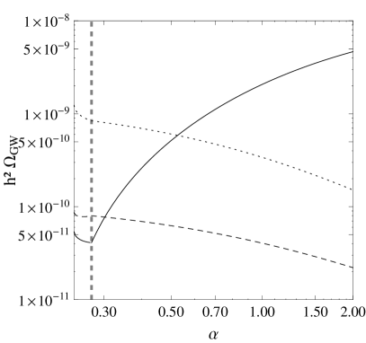
Figure 10: The peak amplitude of the gravitational wave spectrum from bubble collisions (solid line), turbulence (dashed line), and sound waves (dotted line) as functions of $\alpha$, for $g_{*}=100$, $\Delta t=0.1$, and the rest of the parameters as in Figs. 6-8. The vertical line separates detonations from runaway solutions.

We see that the decrease of $\kappa_{\mathrm{fl}}(\alpha)$ is reflected in the GW amplitudes, even though the latter depend on the product $\kappa_{\mathrm{fl}}(\alpha)\,\alpha$. Indeed, the signals from fluid motions generally decrease with $\alpha$, while the signal from bubble wall collisions grows in the runaway regime due to the increase of $\kappa_{\mathrm{wall}}$.

It is important to notice that this behavior of the GW signals with the quantity $\alpha$ was obtained by fixing several parameters, such as the friction coefficients $\eta_{NR},\eta_{UR}$, the bag parameter $\alpha_{c}=\varepsilon/(aT_{c}^{4})$ (which is equivalent to fixing $a_{-}/a_{+}$), as well as the time scale $\Delta t$. In a concrete model, all these quantities will vary together with $\alpha$, as all of them depend on the model parameters. We shall consider concrete models elsewhere. In any case, values of $\alpha$ in the range $0.3\lesssim\alpha\lesssim 1$ are possible in a very strong electroweak phase transition. Hence, Fig. 10 shows that the GWs generated by any of the mechanisms at this phase transition may be observable by eLISA.

6 Conclusions

Several hydrodynamic modes are possible for the growth of a bubble in a cosmological first-order phase transition. These include steady-state walls propagating as deflagrations or detonations [23], accelerated (runaway) walls [17], or even turbulent motion associated with wall corrugation [13]. Which of these propagation modes will a phase transition front take, depends on several factors, such as the amount of supercooling and the friction of the bubble wall with the plasma. In this work we have studied the fastest of these modes, namely, ultra-relativistic detonations and runaway solutions, which may give an important gravitational wave signal from the phase transition.

The generation of gravitational waves depends on the released energy, which is usually measured by the ratio $\alpha$ of the vacuum energy density to the radiation energy density. It is also important how this energy is distributed, as the wall moves, among the bubble wall and the fluid. For a steady-state wall, all the released energy goes to the fluid, either to reheating or to bulk motions. The fraction $\kappa_{\mathrm{fl}}$ of the released vacuum energy which goes into bulk motions is relevant for the formation of gravitational waves through turbulence or sound waves. For runaway walls, there is also a fraction $\kappa_{\mathrm{wall}}$ of the vacuum energy which goes into kinetic energy of the wall. This is relevant for gravitational wave generation from direct bubble collisions. Thus, $\kappa_{\mathrm{fl}}$ is an efficiency coefficient for the injection of kinetic energy in the fluid, while $\kappa_{\mathrm{wall}}$ is as an efficiency coefficient for accelerating the wall.

We have studied, on the one hand, the hydrodynamics of a phase transition front, for given values of the wall velocity and acceleration, i.e., considering these variables as free parameters. Thus, we obtained results for $\kappa_{\mathrm{wall}}$ and $\kappa_{\mathrm{fl}}$ as functions of the velocity $v_{w}$ and the net force $F_{\mathrm{net}}$ acting on the wall. In this way, the results do not depend on the very involved computation of the wall dynamics, for which several approximations are generally needed. On the other hand, we have also studied the wall dynamics, taking into account the back-reaction of hydrodynamics on the wall motion, and we have discussed on the calculation of the wall velocity and acceleration as functions of thermodynamic and friction parameters.

We have computed the efficiency factor $\kappa_{\mathrm{fl}}$ for different wall symmetries, namely, spherical, cylindrical and planar walls. This complements the work of Ref. [24], where we performed a similar analysis for stationary solutions. Here we considered the runaway case. For planar walls we obtained analytic results. The result for spherical bubbles is quite similar to the planar case, which can thus be used as an analytic approximation for the former. Besides, we provide fits for the spherical case as functions of $v_{w}$, $F_{\mathrm{net}}$, and thermodynamic parameters.

For the analysis of the wall dynamics, we considered a phenomenological model for the friction, which was introduced in Ref. [21] and depends on two free parameters. Thus, the model can reproduce the correct value of the friction force in the NR limit, $F_{\mathrm{fr}}\sim\eta_{NR}\,v_{w}$ as well as in the UR limit, $F_{\mathrm{fr}}\sim\eta_{UR}$. In the UR case it is actually more straightforward, for a given model, to compute the net force $F_{\mathrm{net}}$. The determination of the friction component of the UR force is relevant for the use of this phenomenological interpolation, which allows to calculate the wall velocity away from the UR limit. We have clarified the decomposition of $F_{\mathrm{net}}$ into driving and friction forces, taking hydrodynamics effects correctly into account.

Some of the issues discussed in the present paper were previously considered in Ref. [20] (for the case of spherical walls). However, a simpler phenomenological friction was used in that work, which depends on a single friction coefficient, corresponding to the particular case $\eta_{NR}=\eta_{UR}$. Moreover, some results, particularly those for the efficiency factor in the runaway regime, are given in terms of this friction coefficient (cf. Figs. 10 and 12 in [20]). Therefore, those results depend on the wall dynamics. As we have seen, the effect of reheating on the driving force was neglected in Ref. [20], which leads to a different distribution of the released energy. Concrete expressions for the runaway efficiency factors are given in [20] as functions of $\alpha$ and the UR detonation limits $\alpha_{0},\kappa^{\mathrm{det}}_{UR}$. In contrast, we obtained these quantities directly as functions of $\alpha$ and $F_{\mathrm{net}}$. Thus, we provide clean results for $\kappa_{\mathrm{wall}}$ and $\kappa_{\mathrm{fl}}$, which can be used to compute the production of gravitational waves in a phase transition.

In physical models, strongly first-order phase transitions (i.e., those with a relatively high value of the order parameter, $\phi>T$), generally have large amounts of released energy and considerable supercooling. This gives large values of $\alpha$, as well as high wall velocities or even runaway walls. We have explored the efficiency factors and the generation of gravitational waves for such parameter variations.

For detonations and runaway walls, the efficiency factor $\kappa_{\mathrm{fl}}$ decreases with the wall velocity and acceleration, while it increases with the quantity $\alpha$. However, for given values of the friction parameters, $v_{w}$ and $F_{\mathrm{net}}$ are increasing functions of $\alpha$, and it turns out that $\kappa_{\mathrm{fl}}$ decreases with $\alpha$. In contrast, $\kappa_{\mathrm{wall}}$ increases with $F_{\mathrm{net}}$ and $\alpha$. As a consequence, the gravitational wave production through fluid motions generally decreases with $\alpha$, while the production through bubble collisions generally increases. This does not mean, though, that stronger phase transitions will be less efficient in producing gravitational waves through fluid motions. In our parameter variations we have fixed some quantities which, for a concrete model, will change as $\alpha$ changes. In Ref. [30] the electroweak phase transition was considered for several extensions of the Standard Model (all of which gave steady-state walls). In those cases, stronger phase transitions gave stronger GW signals from fluid motions. We shall consider models with even stronger phase transitions in a forthcoming paper [31]. As we have seen, for parameters which are characteristic of such strongly first-order electroweak phase transitions, the gravitational waves may be observed in the planned observatory eLISA.

Appendix A Approximations for the fluid efficiency factor

In Ref. [24] the hydrodynamics was studied for the stationary case, for spherical, cylindrical and planar walls. Although the fluid profiles are different in the three cases (corresponding to the spreading of the released energy in 3, 2, and 1 dimensions, respectively), the total energy in fluid motions is quite similar, particularly for detonations. Therefore, a relatively good approximation for the efficiency factor is to consider a planar wall, for which one obtains analytic results. One expects the same to hold for runaway walls.

For planar symmetry, the shape of the rarefaction wave behind the wall is quite simple. We have constant fluid velocity and enthalpy between the wall and a point which follows the wall with velocity $v_{0}=(v_{-}+c_{-})/(1+v_{-}c_{-})$. Hence, the rarefaction actually begins behind that point. In the variable $\xi=z/t$, this point lies at a fixed position $\xi=v_{0}$, while the wall is at $\xi=v_{w}$. Between $\xi=c_{-}$ and $\xi=v_{0}$ we have

$$v=\frac{\xi-c_{-}}{1-c_{-}\xi},\quad w=w_{-}\left(\frac{1-v_{-}}{1+v_{-}}\frac{1+v}{1-v}\right)^{\frac{1}{2}(c_{-}+\frac{1}{c_{-}})}.$$ (73)

For the bag EOS, we have $c_{-}=1/\sqrt{3}$, and the values of $v_{-}$ and $w_{-}$ are given by Eqs. (27-28) for detonations and by Eqs. (32) for runaway walls. For this profile, the integral $I(v_{w},v_{-})$ in Eqs. (37-39) is given by [24]

$$I=\gamma_{-}^{2}v_{-}^{2}\left(v_{w}-v_{0}\right)+\frac{3\left(2-\sqrt{3}\right)^{\frac{2}{\sqrt{3}}}}{4}\left[\frac{1-v_{-}}{1+v_{-}}\right]^{\frac{2}{\sqrt{3}}}\left[f\left(v_{0}\right)-f\left(c_{-}\right)\right],$$ (74)

where $f\left(\xi\right)=\left(\frac{1+\xi}{1-\xi}\right)^{\frac{2}{\sqrt{3}}}\left\{\frac{2}{\sqrt{3}}-1+\left(1-\xi\right)\left[2-\,_{2}F_{1}(1,1,\frac{2}{\sqrt{3}}+1,\frac{1+\xi}{2})\right]\right\}$, and ${}_{2}F_{1}$ is the hypergeometric function [32]. The efficiency factors $\kappa^{\mathrm{det}}_{\mathrm{pl}},\kappa^{\mathrm{run}}_{\mathrm{pl}}$ for the planar case are obtained by inserting Eq. (74) in Eq. (37) (with $j=0$) or directly in Eq. (39) for the runaway case. The result is shown in Fig. 4, together with that for spherical walls.

Since the planar and spherical results are so similar, we may construct a fit for the spherical case by just approximating the difference between the two results. Indeed, correcting the planar results with a factor $1.03+0.1\sqrt{v_{w}-v_{J}(\alpha)}$ is a good approximation. We thus have

$$\kappa_{\mathrm{fl}}^{\mathrm{det}} = \kappa^{\mathrm{det}}_{\mathrm{pl}}(\alpha,v_{w})\left(1.03+0.1\sqrt{v_{w}-v_{J}(\alpha)}\right),$$ (75)

$$\kappa_{\mathrm{fl}}^{\mathrm{run}} = \kappa^{\mathrm{run}}_{\mathrm{pl}}(\alpha,\bar{F})\left(1.03+0.1\sqrt{1-v_{J}(\alpha)}\right).$$ (76)

In Fig. 11 we compare these fits with the numerical result. In the whole detonation range, and for $F_{\mathrm{net}}/\varepsilon<0.9$ in the runaway case, the relative error is smaller than a 3%.

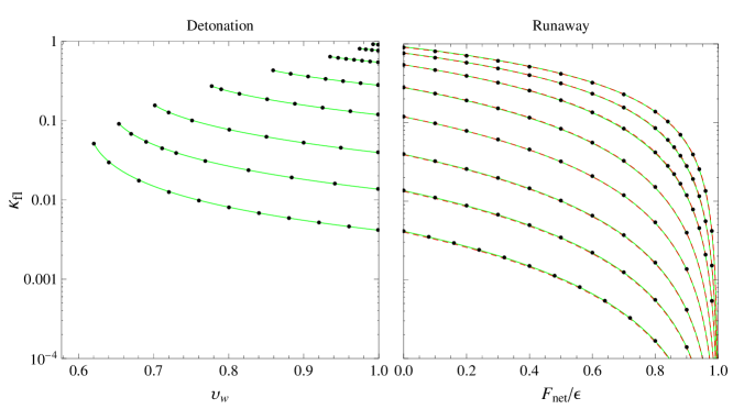
Figure 11: Fits for the efficiency factor for spherical walls, corresponding (from bottom to top) to $\alpha=0.003,0.01,0.03,0.1,0.3,1,3,10$. The black dots indicate values of the numerical result. Red dashed lines correspond to the fit of Eq. (77), and green lines to the fits of Eqs. (75-76).

In the runaway regime it is easy to find a simple fit (which does not rely on the analytic formulas of the planar case), since the integral $I_{1}(v_{-})=I(1,v_{-})$ depends on the single parameter $v_{-}$. In the whole range $0<v_{-}<1$, this function is well approximated by the polynomial $I_{1}(v_{-})\simeq 0.15v_{-}^{2}-0.132v_{-}^{3}+0.065v_{-}^{4}$, with a relative error which is smaller than a 3% for $v_{-}>10^{-3}$. Inserting in Eq. (39), we have

$$\kappa_{\mathrm{fl}}^{\mathrm{run}}\simeq(4/\alpha)(1+3\alpha-3\bar{F})(0.15v_{-}^{2}-0.132v_{-}^{3}+0.065v_{-}^{4})\,,$$ (77)

with $v_{-}(\alpha,\bar{F})$ given by Eq. (32). The result is shown in the right panel of Fig. 11.

References

- [1] For a recent review, see T. Konstandin, Phys. Usp. 56, 747 (2013) [Usp. Fiz. Nauk 183, 785 (2013)] [arXiv:1302.6713 [hep-ph]].
- [2] A. Kosowsky, M. S. Turner and R. Watkins, Phys. Rev. Lett. 69, 2026 (1992); M. Kamionkowski, A. Kosowsky and M. S. Turner, Phys. Rev. D 49, 2837 (1994).
- [3] A. Kosowsky and M. S. Turner, Phys. Rev. D 47, 4372 (1993); C. Caprini, R. Durrer and G. Servant, Phys. Rev. D 77, 124015 (2008) [arXiv:0711.2593 [astro-ph]].
- [4] S. J. Huber and T. Konstandin, JCAP 0809, 022 (2008) [arXiv:0806.1828 [hep-ph]].
- [5] A. D. Dolgov, D. Grasso and A. Nicolis, Phys. Rev. D 66, 103505 (2002); G. Gogoberidze, T. Kahniashvili and A. Kosowsky, Phys. Rev. D 76, 083002 (2007); T. Kahniashvili, G. Gogoberidze and B. Ratra, arXiv:0802.3524 [astro-ph]; L. Kisslinger and T. Kahniashvili, Phys. Rev. D 92, no. 4, 043006 (2015) [arXiv:1505.03680 [astro-ph.CO]].
- [6] C. Caprini, R. Durrer and G. Servant, JCAP 0912, 024 (2009) [arXiv:0909.0622 [astro-ph.CO]];
- [7] C. Caprini, R. Durrer and X. Siemens, Phys. Rev. D 82, 063511 (2010) [arXiv:1007.1218 [astro-ph.CO]].
- [8] M. Hindmarsh, S. J. Huber, K. Rummukainen and D. J. Weir, Phys. Rev. Lett. 112, 041301 (2014) [arXiv:1304.2433 [hep-ph]]; M. Hindmarsh, S. J. Huber, K. Rummukainen and D. J. Weir, arXiv:1504.03291 [astro-ph.CO].
- [9] P. J. Steinhardt, Phys. Rev. D 25, 2074 (1982); M. Laine, Phys. Rev. D 49, 3847 (1994) [arXiv:hep-ph/9309242]; H. Kurki-Suonio and M. Laine, Phys. Rev. D 54, 7163 (1996) [hep-ph/9512202].
- [10] J. Ignatius, K. Kajantie, H. Kurki-Suonio and M. Laine, Phys. Rev. D 49, 3854 (1994) [arXiv:astro-ph/9309059].
- [11] A. Mégevand and A. D. Sánchez, Nucl. Phys. B 820, 47 (2009) [arXiv:0904.1753 [hep-ph]].
- [12] T. Konstandin and J. M. No, JCAP 1102, 008 (2011) [arXiv:1011.3735 [hep-ph]].
- [13] B. Link, Phys. Rev. Lett. 68, 2425 (1992); P. Y. Huet, K. Kajantie, R. G. Leigh, B. H. Liu and L. D. McLerran, Phys. Rev. D 48, 2477 (1993); M. Abney, Phys. Rev. D 49, 1777 (1994); L. Rezzolla, Phys. Rev. D 54, 1345 (1996); A. Megevand and F. A. Membiela, Phys. Rev. D 89, 103507 (2014); A. Megevand, F. A. Membiela and A. D. Sanchez, JCAP 1503, no. 03, 051 (2015) [arXiv:1412.8064 [hep-ph]].
- [14] A. Megevand and F. A. Membiela, Phys. Rev. D 89, 103503 (2014).
- [15] G. D. Moore and T. Prokopec, Phys. Rev. D 52, 7182 (1995) [arXiv:hep-ph/9506475]; Phys. Rev. Lett. 75, 777 (1995) [arXiv:hep-ph/9503296];
- [16] B. H. Liu, L. D. McLerran and N. Turok, Phys. Rev. D 46, 2668 (1992); N. Turok, Phys. Rev. Lett. 68, 1803 (1992); M. Dine, R. G. Leigh, P. Y. Huet, A. D. Linde and D. A. Linde, Phys. Rev. D 46, 550 (1992) [arXiv:hep-ph/9203203]; S. Y. Khlebnikov, Phys. Rev. D 46, 3223 (1992); P. Arnold, Phys. Rev. D 48, 1539 (1993) [arXiv:hep-ph/9302258]; P. John and M. G. Schmidt, Nucl. Phys. B 598, 291 (2001) [Erratum-ibid. B 648, 449 (2003)]; G. D. Moore, JHEP 0003, 006 (2000); J. Kozaczuk, JHEP 1510, 135 (2015) [arXiv:1506.04741 [hep-ph]].
- [17] D. Bodeker and G. D. Moore, JCAP 0905, 009 (2009) [arXiv:0903.4099 [hep-ph]].
- [18] S. J. Huber and M. Sopena, arXiv:1302.1044 [hep-ph].
- [19] T. Konstandin, G. Nardini and I. Rues, JCAP 1409, no. 09, 028 (2014).
- [20] J. R. Espinosa, T. Konstandin, J. M. No and G. Servant, JCAP 1006, 028 (2010) [arXiv:1004.4187 [hep-ph]];
- [21] A. Megevand, JCAP 1307, 045 (2013).
- [22] H. Kurki-Suonio, Nucl. Phys. B 255, 231 (1985).
- [23] M. Gyulassy, K. Kajantie, H. Kurki-Suonio and L. D. McLerran, Nucl. Phys. B 237 (1984) 477; K. Kajantie and H. Kurki-Suonio, Phys. Rev. D 34, 1719 (1986); K. Enqvist, J. Ignatius, K. Kajantie and K. Rummukainen, Phys. Rev. D 45, 3415 (1992); H. Kurki-Suonio and M. Laine, Phys. Rev. D 51, 5431 (1995) [arXiv:hep-ph/9501216]; A. Megevand, Phys. Rev. D 78, 084003 (2008) [arXiv:0804.0391 [astro-ph]].
- [24] L. Leitao and A. Mégevand, Nucl. Phys. B 844, 450 (2011) [arXiv:1010.2134 [astro-ph.CO]].
- [25] L. Leitao and A. Megevand, Nucl. Phys. B 891, 159 (2015) [arXiv:1410.3875 [hep-ph]].
- [26] M. Quiros, arXiv:hep-ph/9901312.
- [27] A. Megevand and A. D. Sánchez, Nucl. Phys. B 825, 151 (2010).
- [28] P. A. Seoane et al. [eLISA Collaboration], arXiv:1305.5720 [astro-ph.CO].
- [29] C. Caprini et al., arXiv:1512.06239 [astro-ph.CO].
- [30] L. Leitao, A. Megevand and A. D. Sánchez, JCAP 1210, 024 (2012).
- [31] L. Leitao and A. Megevand, arXiv:1512.08962 [astro-ph.CO].
- [32] I. S. Gradshteyn and I.M. Ryzhik, Table of Integrals, Series, and Products (Academic Press, San Diego, 2000).