On the evolution of a rogue wave along the orthogonal direction of the ($t,x$)-plane

Abstract.

The localization characters of the first-order rogue wave (RW) solution $u$ of the Kundu-Eckhaus equation is studied in this paper. We discover a full process of the evolution for the contour line with height $c^{2}+d$ along the orthogonal direction of the ($t,x$)-plane for a first-order RW $|u|^{2}$: A point at height $9c^{2}$ generates a convex curve for $3c^{2}\leq d<8c^{2}$, whereas it becomes a concave curve for $0<d<3c^{2}$, next it reduces to a hyperbola on asymptotic plane (i.e. equivalently $d=0$), and the two branches of the hyperbola become two separate convex curves when $-c^{2}<d<0$, and finally they reduce to two separate points at $d=-c^{2}$. Using the contour line method, the length, width, and area of the RW at height $c^{2}+d(0<d<8c^{2})$ , i.e. above the asymptotic plane, are defined. We study the evolutions of three above-mentioned localization characters on $d$ through analytical and visual methods. The phase difference between the Kundu-Eckhaus and the nonlinear Schrodinger equation is also given by an explicit formula.

Keywords: rogue wave, localization characters, contour line method.

PACS numbers: 02.30.Ik,03.75.Lm,42.65.Tg

1. Introduction

The nonlinear Schrödinger(NLS) equation, one of the most famous equation in physics, is as follows [1, 2],

$$i\,u_{t}+u_{xx}+2\,|u|^{2}\,u=0,$$ (1)

which has been studied extensively from the point of view of mathematics and physics [3, 4]. Here, $u(x,t)$ is the envelope of an electric field, $t$ denotes the normalized spatial variable and $x$ is the normalized time variable. Nevertheless, in order to get high bit rates in optical fiber communication system, one always has to increase the intensity of the incident light field to produce ultrashort (femtosecond or even attosecond) optical pulses. In this case, a simple NLS equation is inadequate to accurately describe the propagation of light in fiber, and high-order nonlinear effects, such as third-order dispersion, self-steepening, and self-frequency shift, must be taken into consideration [5, 6]. To model above highly nonlinear optical system, we have to add higher-order nonlinear terms and its derivatives into the NLS equation. It is a big challenge to do this corrections of the NLS equation without loss of the integrability. Regarding the inclusion of above ideas, the Kundu-Eckhaus(KE) equation [7, 8], which was introduced as a cubic-quintic extension of the NLS equation and also can be reduced from several models of optics [9, 10, 11, 12, 13] and fluid [14], is one of the well-known examples. The KE equation is given in the form of [7]

$$i\,u_{t}+u_{xx}+2\,|u|^{2}\,u+4\,\beta^{2}\,|u|^{4}\,u-4i\,\beta\left(|u|^{2}\right)_{x}u=0,\quad\beta\in\mathbf{R},$$ (2)

which contains higher nonlinearity and the Raman effect in nonlinear optics. $\beta$ is a real constant, $\beta^{2}$ is the quinic nonlinear coefficient, and the last term is responsible for the self-frequency shift. The integrability aspects of KE equation has been extensively studied by using the explicit form of the Lax pair, Painleve property [15], Hamiltonian structure [16], soliton solutions obtained through the Darboux transformation (DT) [17] and by the bilinear method [18] and by a direct method [19], higher-order extension[20], infinitely many conservation laws[21], lower-order rogue waves (RWs) given by the DT method[22], etc. In particular, the DT of the KE equation is not completely established [17, 22] because there exists an overall factor $A_{A}$(or $\alpha_{N}$) involved with complicated integrations, which produces the difficulty in the construction of multi-fold DT. Very recently, we overcame this problem thoroughly by finding an explicit analytical form of the overall factor $\prod\limits_{i=0}^{n-1}H^{[i]}$ for the n-fold DT $T_{n}$ (see Theorem 2.3 of Ref. [23]). In particular, several higher-order rogue waves of the KE equation have been given explicitly in references [22, 23, 24].

Rogue wave is one kind of common nonlinear local waves which is also called as freak wave, monster wave, killer wave, extreme wave and abnormal wave. It is used to describe spontaneous huge ocean waves, which can lead to water walls taller than 20-30 m so that it is even a threaten to a big ship [25, 26, 27]. The study of rogue wave has been boosted extremely by the laboratory observations in nonlinear fibers [28, 29] and in water tanks [30], then rogue wave has also extended fleetly to many fields such as plasmas, super fluids, capillary flow, Bose-Einstein condensates, the atmosphere [31, 32, 33, 34, 35], etc. In order to better understand and apply the rogue wave concept in any physical system, it is necessary to analyse the features of the rogue wave profiles. Especially, the squared modulus of the solution $|u|^{2}$ always represents a measurable quantity, optical power (or intensity). Recently, a effective tool, contour line method, is applied to study the localization characters of the profile for rogue waves by computing the width, length and area [23, 36, 37, 38]. It is known that the contour line on the asymptotic plane is a hyperbola, while the contour line above the asymptotic plane is a closed curve and then the width, length and area of the rogue wave can be worked out [23]. But in [36, 23, 37, 38], we just analysed the localization characters at a given height $c^{2}+1$ along the orthogonal direction of the ($t,x$)-plane, where $c^{2}$ is the height of asymptotic background for rogue wave $|u|^{2}$. How does these localized characters are evolving along the orthogonal direction of the ($t,x$)-plane ? It’s known that the counter line on the height $c^{2}+1$ along the orthogonal direction of the ($t,x$)-plane is a closed concave curve, for example, see Figure 7(b) of Ref. [23]. But whether the counter line at height $c^{2}+d(0\leq d\leq 8c^{2}$ along the orthogonal direction of the ($t,x$)-plane, we shall explain this constraint later) is always a concave curve, and if it’s not, how to find a critical height $d_{c}$ by changing from a concave contour line to a convex one? Here $d$ denotes the height of counter line from the asymptotic background. These questions will be answered in this paper.

The rest of the paper is organized as follows. In section 2, according to the explicit expression of the first-order rogue wave solution of the KE equation, we provide an algebraic equation to determine the counter line at height $c^{2}+d$ ($8c^{2}\geq d\geq 0$) along the orthogonal direction of the ($t,x$)-plane, and then find the critical height $d_{c}$. The convex profile of the counter lines with height $c^{2}-d(c^{2}\geq d>0)$ along the orthogonal direction of the ($t,x$)-plane is also discussed. In section 3, we work out the width, length and area of the contour line lower than $d_{c}$, and then analyse the influence of the parameters $d$. In section 4, we consider the localization characters of the counter line higher than $d_{c}$. In section 5, we give conclusions and discussions.

2. The critical height $d_{c}$

Through the Darboux transformation, we have generated the first-order rouge wave(RW) of the KE equation [23] in the form

$$u^{[1]}_{rw}=\frac{L_{r1}}{L_{r2}}\exp\left({\rm i}(\rho+\frac{L_{r3}}{L_{r2}})\right),$$ (3)

where

$$L_{r1}=-4\,{c}^{3}{x}^{2}+\left(-32\,\beta\,{c}^{5}+16\,a{c}^{3}\right)tx+\left(-64\,{\beta}^{2}{c}^{7}+64\,a\beta\,{c}^{5}-16\,{a}^{2}{c}^{3}-16\,{c}^{5}\right){t}^{2}+16\,it{c}^{3}+3\,c,$$

$$L_{r2}=\left(64\,{\beta}^{2}{c}^{6}-64\,a\beta\,{c}^{4}+16\,{a}^{2}{c}^{2}+16\,{c}^{4}\right){t}^{2}+\left(32\,\beta\,{c}^{4}-16\,a{c}^{2}\right)xt+4\,{c}^{2}{x}^{2}+1,$$

$$L_{r3}=16\,\beta\,{c}^{2}x+\left(64\,{\beta}^{2}{c}^{4}-32\,a\beta\,{c}^{2}\right)t,\qquad\rho=ax+(-a^{2}+4\beta^{2}c^{4}+2c^{2})t,$$

and $a,c,\beta$ are real constant. It is trivial to find that $|u^{[1]}_{rw}|^{2}$ goes to $c^{2}$ when $|x|\rightarrow\infty$ and $|t|\rightarrow\infty$, which implies that the height of the asymptotic background is $c^{2}$. $|u^{[1]}_{rw}|^{2}$ is a doubly-localized rational function with a large amplitude $9c^{2}$ at (0,0) on ($t,x$)-plane, which reflects the two typical characters of the RW, namely, localization and large amplitude. Figure 1 is plotted for $|u^{[1]}_{rw}|^{2}$ in order to show visibly the above two characteristic features.

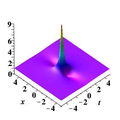
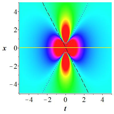
Figure 1. The profile of the first-order RW solutions $|u_{rw}^{[1]}|^{2}$ with $a=0.5,c=1,\beta=0.25$. The panel (b) is the density plot of the panel (a). In panel (b), $l_{1}$ (black, dash) and $l_{2}$ (blue, dot) are two asymptotes, and $l_{3}$ (yellow, solid) is the non-orthogonal axis of the contour line in equation (4).

It is shown from Figure 1 that the counter line above the asymptotic background is reducing from a concave curve to a point when the height $c^{2}+d$ along the orthogonal direction of the ($t,x$)-plane of counter line is raising from $c^{2}$ to $9c^{2}$. Here $d$ denotes the height of contour line from the asymptotic background. This observation of $|u^{[1]}_{rw}|^{2}$ shows that $d$ is a key parameter to control the profile of the contour line, and strongly responsible for the existence of a critical height $d_{c}$ at which we observe interesting transition from a concave contour line to convex one. However, there are already three parameters $a$, $c$ and $\beta$ in the RW $u^{[1]}_{rw}$, and then it is a challenging problem to illustrate analytically the role of $d$ in control of the profile. At present the contour line method is really a useful tool to analyse the localization characters at a given height $c^{2}+1$ (i.e. $d=1$) of the first-order RW solution [23, 36, 37, 38]. In the following context we shall use contour line of $|u^{[1]}_{rw}|^{2}$ with given values of parameters ($a,c,\beta$) to study the evolution of profile with a varying $d$. By this method, a contour line of $|u^{[1]}_{rw}|^{2}$ at height $c^{2}+d$ ($d>0$) along the orthogonal direction of the ($t,x$)-plane is expressed by

$$-16c^{4}dx^{4}+(-256\beta c^{6}d+128ac^{4}d)tx^{3}+R_{1}x^{2}+R_{2}x+R_{3}t^{4}+R_{4}t^{2}+8c^{2}-d=0,$$ (4)

where

$$R_{1}= \left(-1536\,{\beta}^{2}{c}^{8}d+1536\,a\beta\,{c}^{6}d-384\,{a}^{2}{c}^{4}d-128\,{c}^{6}d\right){t}^{2}-32\,{c}^{4}-8\,{c}^{2}d,$$

$$R_{2}= -4096\,{\beta}^{3}{c}^{10}d+6144\,a{\beta}^{2}{c}^{8}d-3072\,{a}^{2}\beta\,{c}^{6}d-1024\,\beta\,{c}^{8}d+512\,{a}^{3}{c}^{4}d+512\,a{c}^{6}d,$$

$$R_{3}= -4096\,{\beta}^{4}{c}^{12}d+8192\,a{\beta}^{3}{c}^{10}d-6144\,{a}^{2}{\beta}^{2}{c}^{8}d-2048\,{\beta}^{2}{c}^{10}d$$

$$+2048\,{a}^{3}\beta\,{c}^{6}d+2048\,a\beta\,{c}^{8}d-256\,{a}^{4}{c}^{4}d-512\,{a}^{2}{c}^{6}d-256\,{c}^{8}d,$$

$$R_{4}= -512\,{\beta}^{2}{c}^{8}-128\,{\beta}^{2}{c}^{6}d+512\,a\beta\,{c}^{6}+128\,a\beta\,{c}^{4}d-128\,{a}^{2}{c}^{4}+128\,{c}^{6}-32\,{a}^{2}{c}^{2}d-32\,{c}^{4}d.$$

Set $d=0$ in Eq.(4), the contour line [23] is a hyperbola on the asymptotic plane which has two asymptotes

$$l_{1}:x=2(a-2\beta c^{2}-c)t,\qquad l_{2}:x=2(a-2\beta c^{2}+c)t,$$

and two non-orthogonal axes

$$major\quad axis:t=0,\qquad imaginary\quad axis(l_{3}):x=(2a-4\beta c^{2})t.$$

These three lines are plotted in Figure 1(b). As the maximum amplitude of $|u_{rw}^{[1]}|^{2}$ is $9c^{2}$, so the height of contour line above the background must be in the interval $(c^{2},9c^{2}]$ or equivalently $0<d\leq 8c^{2}$.

Note that Eq.(4) is an implicit form of the contour line. Actually, it can be expressed explicitly by two branches

$$l_{4}: x=-4\beta c^{2}t+2at+\frac{F_{2}}{2dc},$$ (5)

$$l_{5}: x=-4\beta c^{2}t+2at-\frac{F_{2}}{2dc},$$ (6)

in which $F_{2}=\sqrt{-(16c^{4}d^{2}t^{2}+4c^{2}d+d^{2})+4cd\sqrt{16c^{4}dt^{2}+c^{2}+d}}$ ($t\in[-\frac{\sqrt{d(8c^{2}-d)}}{4dc^{2}},\frac{\sqrt{d(8c^{2}-d)}}{4dc^{2}}])$. Set $F_{2}=\sqrt{-F_{2A}+F_{2B}}$ and $y=t^{2}$, then $F_{2B}^{2}-F_{2A}^{2}=$ $-\left(16\,{c}^{4}y+1\right)\left(16\,{c}^{4}dy-8\,{c}^{2}+d\right)\geq 0$ if $t\in[-\frac{\sqrt{d(8c^{2}-d)}}{4dc^{2}},\frac{\sqrt{d(8c^{2}-d)}}{4dc^{2}}])$, then $F_{2B}-F_{2A}>0$. Thus $F_{2}$ is a real function of $t$. The derivatives with respect to $t$ of two branches are

$$l_{4}:-4\beta c^{2}+2a+\frac{F_{1}}{F_{2}}-x^{\prime}(t)=0,\quad and\quad l_{5}:-4\beta c^{2}+2a-\frac{F_{1}}{F_{2}}-x^{\prime}(t)=0,$$ (7)

with $F_{1}=-8c^{3}dt+\frac{16dc^{4}t}{\sqrt{16c^{4}dt^{2}+c^{2}+d}}$, and $x^{\prime}(t)$ means $\frac{dx}{dt}$.

We are now in a position to find $d_{c}$. It can be realized by finding how many points on $l_{4}$ (or $l_{5}$) whose derivative in Eq.(7) is equal to the slope of $l_{3}$. The slope of the line $l_{3}$ is $k=2a-4\beta c^{2}$. So set $x^{\prime}(t)=k$, Eq.(7) leads to two equivalent equations of $t$

$$-8c^{3}dt(\sqrt{16c^{4}dt^{2}+c^{2}+d}-2c)=0\,(by\,l_{4}),8c^{3}dt(\sqrt{16c^{4}dt^{2}+c^{2}+d}-2c)=0\,(by\,l_{5}).$$ (8)

By solving Eq.(8) we know that $t$ has three values $0$, $\frac{\sqrt{d(3c^{2}-d)}}{4dc^{2}}$, and $-\frac{\sqrt{d(3c^{2}-d)}}{4dc^{2}}$, if $0<d<3c^{2}$; or it just has one value $0$ if $d\geq 3c^{2}$. The former produces a concave contour line at height $c^{2}+d$ along the orthogonal direction of the ($t,x$)-plane, but the latter gives a convex one. Thus the critical value of height is $d_{c}=3c^{2}$. In Figure 2, $d_{c}=3$, thus contour lines associated with $d=0.1$ and $0.2$ (outer) are concave, but $d=3$ and $6$ (inner) gives two convex contour lines.

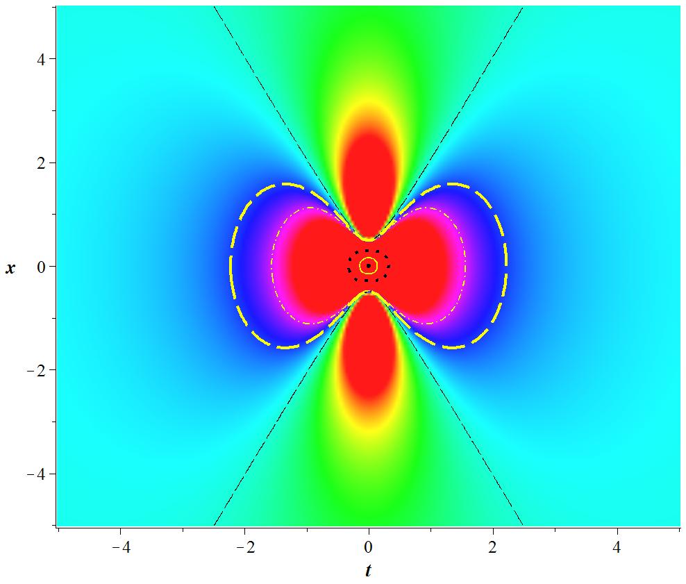
Figure 2. The density plot and contour lines of the first-order RW solution $|u_{rw}^{[1]}|^{2}$ with $a=1/2,c=1,\beta=1/4$. Different values of $d$ from outside to inside: $d=0$ (longdash,thin), $d=0.1$ (dash,thick), $d=0.2$ (dashdot), $d=3$ (dot), $d=6$ (solid), $d=8$ (a point). Note that $|u_{rw}^{[1]}|^{2}$ reaches maximum value $9$ at (0,0), which is corresponding to the point given by contour line at $d=8$. The parameter $d=0$ produces two branches of a hyperbola on the asymptotic plane.

For the contour line of $|u_{rw}^{[1]}|^{2}$ below the asymptotic plane, all detailed calculations of this case are given in appendix. Its height is $c^{2}-d(c^{2}\geq d>0)$ along the orthogonal direction of the ($t,x$)-plane and then the governing equation is Eq.(4) with $-d$ instead of $d$. This implicit equation can be expressed explicitly by four branches, which determines a close contour line in upper half-plane with two end points (see $P_{1}^{{}^{\prime}},P_{2}^{{}^{\prime}}$ in Figure 3) and another in lower half-plane with two end points (see $P_{1}^{{}^{\prime\prime}},P_{2}^{{}^{\prime\prime}}$ in Figure 3). The four points are expressd by

$$P_{2}^{{}^{\prime}}=(-\frac{\sqrt{d(c^{2}-d)}}{4c^{2}d},-\frac{(a-2\beta c^{2})\sqrt{d(c^{2}-d)}-c^{2}\sqrt{3d}}{2c^{2}d}), P_{1}^{{}^{\prime}}=(\frac{\sqrt{d(c^{2}-d)}}{4c^{2}d},\frac{(a-2\beta c^{2})\sqrt{d(c^{2}-d)}+c^{2}\sqrt{3d}}{2c^{2}d}),$$

$$P_{2}^{{}^{\prime\prime}}=(-\frac{\sqrt{d(c^{2}-d)}}{4c^{2}d},-\frac{(a-2\beta c^{2})\sqrt{d(c^{2}-d)}+c^{2}\sqrt{3d}}{2c^{2}d}), P_{1}^{{}^{\prime\prime}}=(\frac{\sqrt{d(c^{2}-d)}}{4c^{2}d},\frac{(a-2\beta c^{2})\sqrt{d(c^{2}-d)}-c^{2}\sqrt{3d}}{2c^{2}d}).$$

The $P_{2}^{{}^{\prime}}P_{1}^{{}^{\prime}}$ is parallel to $P_{2}^{{}^{\prime\prime}}P_{1}^{{}^{\prime\prime}}$, and their slope is the same as $l_{3}$. By a similar way as discussed in the last paragraph, it is not difficult to show that two separate counter lines (see Figure 3) are convex for all values of $d(c^{2}>d>0)$, unlike the counter line with height $c^{2}+d(8c^{2}>d>0)$ which has a critical value $d_{c}$ at which change occurs from a concave profile to a convex one. Figure 4 is plotted for the contour lines with different height $d$ below the asymptotic plane, and the resulting curves are convex and separate, which gives a visual confirmation of our above results. Two centers of valleys are $(0,\,{\frac{\sqrt{3}}{2c}})$ and $(0,\,-{\frac{\sqrt{3}}{2c}})$ (see two points in this figure), and their values are zero.

According to the above study with the help of analytical way, we obtain a full process of the evolution for the counter line with height $c^{2}+d$ along the orthogonal direction of the ($t,x$)-plane for a first-order RW $|u_{rw}^{[1]}|^{2}$: A point at height $9c^{2}$ generates a convex curve for $3c^{2}\leq d<8c^{2}$, whereas it becomes a concave curve for $0<d<3c^{2}$, next it reduces to a hyperbola on asymptotic plane (i.e. equivalently $d=0$), and the two branches of the hyperbola become two separate convex curves when $-c^{2}<d<0$, and finally they reduce to two separate points at $d=-c^{2}$. Note again on ($t,x$)-plane that the maximum peak is located at ($0,0$), and two minimum points are located at $(0,\,{\frac{\sqrt{3}}{2c}})$ and $(0,\,-{\frac{\sqrt{3}}{2c}})$,

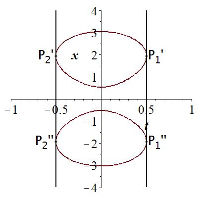
Figure 3. End points of contour lines for $|u_{rw}^{[1]}|^{2}$ below the asymptotic plane with height $c^{2}-d$. The governing equation of these contour lines is Eq.(4) with $-d$ instead of $d$. Parameters are given by $a=1/2$, $c=1$, $d=1/5$, $\beta=1/4$. Four end points are $P_{1}^{\prime}=(\frac{1}{2},\frac{\sqrt{15}}{2}),P_{2}^{\prime}=(-\frac{1}{2},\frac{\sqrt{15}}{2}),P_{1}^{\prime\prime}=(\frac{1}{2},-\frac{\sqrt{15}}{2}),P_{2}^{\prime\prime}=(-\frac{1}{2},-\frac{\sqrt{15}}{2})$ on the ($t,x$)-plane.

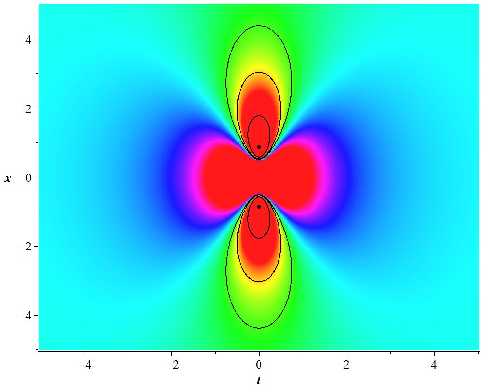
Figure 4. The contour line of the first-order RW solution $|u_{rw}^{[1]}|^{2}$ with height $c^{2}-d$. The governing equation of the contour line is Eq.(4) with $-d$ instead of $d$. Parameters: $a=1/2,c=1,\beta=1/4$. Different values of $d$ from outside to inside: $d=0.1$, $d=0.2$, $d=0.5$, $d=1$. Two points are given by $d=1$, which are located at ($0,\,{\frac{\sqrt{3}}{2}}$) and ($0,\,-{\frac{\sqrt{3}}{2}}$) on ($t,x$)-plane.

3. The contour line below the critical value

In this section, we consider the localization characters of the first-order RW when $0<d<3c^{2}$. According to explicit formulas Eqs.(5, 6) of two branches for contour line (see Figure 5), two end points on the ($t,x$)-plane are $P_{1}=\left(\frac{\sqrt{d(8c^{2}-d)}}{4dc^{2}},\frac{(2a-4\beta c^{2})\sqrt{d(8c^{2}-d)}}{4dc^{2}}\right)$, $P_{2}=\left(-\frac{\sqrt{d(8c^{2}-d)}}{4dc^{2}},-\frac{(2a-4\beta c^{2})\sqrt{d(8c^{2}-d)}}{4dc^{2}}\right)$, for all values of $a$, $c$ and $\beta$. And the equations of $BC$ and $AD$ (see Figure 5) are given below,

$$BC:\qquad t=-\frac{\sqrt{d(8c^{2}-d)}}{4dc^{2}},\qquad AD:\qquad t=\frac{\sqrt{d(8c^{2}-d)}}{4dc^{2}}.$$ (9)

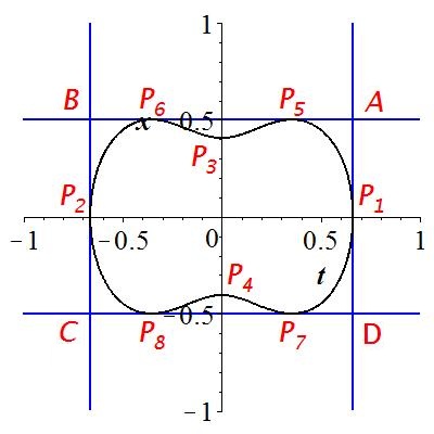
Figure 5. The tangent lines of the contour for the first-order RW solution $|u_{rw}^{[1]}|^{2}$ with $a=\frac{1}{2}$, $c=1$, $d=1$, $\beta=\frac{1}{4}$.

The length of the first-order RW solution $|u_{rw}^{[1]}|^{2}$ at height $d$ is defined by the distance of $P_{1}$ and $P_{2}$ [36],

$$d_{LKE}=\frac{1}{2}\sqrt{\frac{(4(a-2\beta c^{2})^{2}+1)(8c^{2}-d)}{c^{4}d}}.$$ (10)

For contour line in Eq.(4) (or equivalently in Eqs.(5, 6)) with the condition $d\leq d_{c}$, there are three values of $t$ at $0,\frac{\sqrt{d(3c^{2}-d)}}{4dc^{2}},-\frac{\sqrt{d(3c^{2}-d)}}{4dc^{2}}$, which imply six extreme points (see Figure 5) at

$$P_{3}=\left(0,\frac{\sqrt{-4c^{2}d-d^{2}+4d\sqrt{c^{4}+c^{2}d}}}{2dc}\right),$$

$$P_{4}=\left(0,-\frac{\sqrt{-4c^{2}d-d^{2}+4d\sqrt{c^{4}+c^{2}d}}}{2dc}\right),$$

$$P_{5}=\left({\frac{\sqrt{d\left(3\,{c}^{2}-d\right)}}{4{c}^{2}d}},\frac{(a-2\beta c^{2})\sqrt{d(3c^{2}-d)}+c^{2}\sqrt{d}}{2c^{2}d}\right),$$

$$P_{6}=\left(-{\frac{\sqrt{d\left(3\,{c}^{2}-d\right)}}{4{c}^{2}d}},\frac{-(a-2\beta c^{2})\sqrt{d(3c^{2}-d)}+c^{2}\sqrt{d}}{2c^{2}d}\right),$$

$$P_{7}=\left({\frac{\sqrt{d\left(3\,{c}^{2}-d\right)}}{4{c}^{2}d}},\frac{(a-2\beta c^{2})\sqrt{d(3c^{2}-d)}-c^{2}\sqrt{d}}{2c^{2}d}\right),$$

$$P_{8}=\left(-{\frac{\sqrt{d\left(3\,{c}^{2}-d\right)}}{4{c}^{2}d}},\frac{-(a-2\beta c^{2})\sqrt{d(3c^{2}-d)}-c^{2}\sqrt{d}}{2c^{2}d}\right).$$

By a simple calculation, it shows $-4c^{2}d-d^{2}+4d\sqrt{c^{4}+c^{2}d}>0$ if $d\in(0,8c^{2})$, so all coordinates of $P_{i}(i=3,\cdots,8)$ are well defined. Note here $d<d_{c}=3c^{2}$. The equations of $AB$ and $CD$ are as follows:

$$AB:\qquad x-(2a-4\beta c^{2})t-\frac{1}{2\sqrt{d}}=0,$$ (11)

$$CD:\qquad x-(2a-4\beta c^{2})t+\frac{1}{2\sqrt{d}}=0.$$ (12)

The width of the first-order RW solution $|u_{rw}^{[1]}|^{2}$ at height $d$ there upon is defined by the distance of $AB$ and $CD$, which is in the form of

$$d_{WKE}=\frac{1}{\sqrt{d(4(a-2\beta c^{2})^{2}+1)}}.$$ (13)

Further the area of the first-order RW solution $|u_{rw}^{[1]}|^{2}$ at height $d$ is defined by the area of the outer tangent parallelogram of the contour line, i.e.

$$S_{ABCD}=d_{LKE}d_{WKE}=\frac{\sqrt{8c^{2}-d}}{2c^{2}d}.$$ (14)

Comparing Eq.(10) with Eq.(13), there exists a condition $\beta=\frac{a}{2c^{2}}$ which implies a minimum $d_{LKE_{min}}=\frac{1}{2}\sqrt{\frac{8c^{2}-d}{c^{4}d}}$ of the length and a maximum $d_{WKE_{max}}=\frac{1}{\sqrt{d}}$ of the width. It is interesting to note that the condition for extreme value is independent of $d$. If $d=4c^{2}(2-c^{2})$ and $c\in(\frac{\sqrt{5}}{2},\sqrt{2})$, $d_{LKE_{min}}=d_{WKE_{max}}$. In Figure 6(a), there is no crossing point because $c\notin(\frac{\sqrt{5}}{2},\sqrt{2})$, but Figure 6(b) has one crossing point at $2.096$.

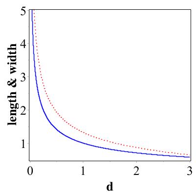
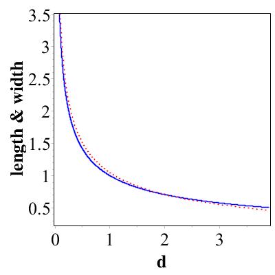
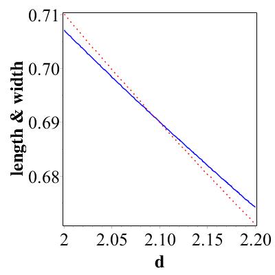
Figure 6. The minimum of length $d_{LKE_{min}}$ (red,dot) and the maximum of width $d_{WKE_{max}}$(blue,solid) of the contour line above the critical height $d_{c}$. In panel (a), $c=1$, and there is no crossing point. In panels (b, c), $c=1.3$, the latter is the local picture of the former, and the crossing point is given at $d=2.096$.

For $\beta\not=\frac{a}{2c^{2}}$, we do not analyse the condition of $d_{LKE}=d_{WKE}$ because of its complexity, and then Figure 7 is plotted to show the evolution of three localization characters on $d$.

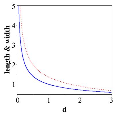
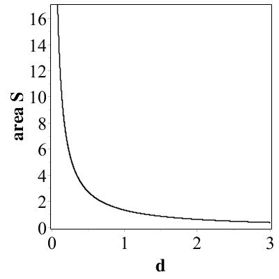
Figure 7. The length $d_{LKE}$ (red,dot) and width $d_{WKE}$(blue,solid) and the area $S$ of the contour line below the critical height $d_{c}$ with parameters $a=1/2,c=1,\beta=0.30$. There is no crossing point in panel (a).

4. The contour line above the critical value

In this section, we consider the localization characters of the first RW when $3c^{2}\leq d<8c^{2}$ along the orthogonal direction of the ($t,x$)-plane. Within this region, the contour line also has two end points $Q_{1}=\left(\frac{\sqrt{d(8c^{2}-d)}}{4dc^{2}},\frac{(2a-4\beta c^{2})\sqrt{d(8c^{2}-d)}}{4dc^{2}}\right)$, $Q_{2}=\left(-\frac{\sqrt{d(8c^{2}-d)}}{4dc^{2}},-\frac{(2a-4\beta c^{2})\sqrt{d(8c^{2}-d)}}{4dc^{2}}\right)$, on the ($t,x$) plane of all values of $a$ , $c$ and $\beta$. And the equations of $B^{{}^{\prime}}C^{{}^{\prime}}$ and $A^{\prime}D^{\prime}$ is given below,

$$B^{{}^{\prime}}C^{{}^{\prime}}:\qquad t=-\frac{\sqrt{d(8c^{2}-d)}}{4dc^{2}},\qquad A^{{}^{\prime}}D^{{}^{\prime}}:\qquad t=\frac{\sqrt{d(8c^{2}-d)}}{4dc^{2}}.$$ (15)

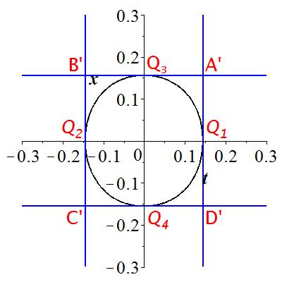
Figure 8. The tangent lines of the contour of the first-order RW solution $|u_{rw}^{[1]}|^{2}$ with $a=0.5$, $c=1$, $d=6$, $\beta=0.25$

The length of the first-order RW solution $|u_{rw}^{[1]}|^{2}$ is the distance of $Q_{1}$ and $Q_{2}$ (see Figure8 ), i.e.

$$d_{LKE}^{{}^{\prime}}=\frac{1}{2}\sqrt{\frac{(4(a-2\beta c^{2})^{2}+1)(8c^{2}-d)}{c^{4}d}}.$$ (16)

The length in Eq.(16) is the same as the counter line below the critical value, but the other two localization characters (i.e. width and area) are different for two cases. If $d\geq 3c^{2}$ , the Eq.(8) has only one solution, i.e. $t=0$. So points $P_{5}$ and $P_{6}$ are approaching to point $P_{3}=Q_{3}=\left(0,\frac{\sqrt{-4c^{2}d-d^{2}+4d\sqrt{c^{4}+c^{2}d}}}{2dc}\right)$ when $d$ is passing by $d_{c}$ from a lower height. Similarly, points $P_{7}$ and $P_{8}$ are approaching to point $P_{4}=Q_{4}=\left(0,-\frac{\sqrt{-4c^{2}d-d^{2}+4d\sqrt{c^{4}+c^{2}d}}}{2dc}\right)$. We can work out the equations of $A^{{}^{\prime}}B^{{}^{\prime}}$ and $C^{{}^{\prime}}D^{{}^{\prime}}$ (see Figure8) as

$$A^{{}^{\prime}}B^{{}^{\prime}}:\qquad x-(2a-4\beta c^{2})t+\frac{\sqrt{-4c^{2}d-d^{2}+4d\sqrt{c^{4}+c^{2}d}}}{2dc}=0,$$ (17)

$$C^{{}^{\prime}}D^{{}^{\prime}}:\qquad x-(2a-4\beta c^{2})t-\frac{\sqrt{-4c^{2}d-d^{2}+4d\sqrt{c^{4}+c^{2}d}}}{2dc}=0.$$ (18)

The width of the rogue wave $|u_{rw}^{[1]}|^{2}$ at height $d$ is defined by the distance of above two lines, which is

$$d_{WKE}^{{}^{\prime}}=\sqrt{\frac{4c\sqrt{c^{2}+d}-4c^{2}-d}{c^{2}d(4(a-2\beta c^{2})^{2}+1)}}.$$ (19)

The area of the rogue wave $|u_{rw}^{[1]}|^{2}$ at height $d$ is defined by the area of the outer tangent parallelogram (see Figure 8) of its contour line at same height, which is given by

$$S_{ABCD}^{{}^{\prime}}=d_{LKE}^{{}^{\prime}}d_{WKE}^{{}^{\prime}}=\frac{\sqrt{(4c\sqrt{c^{2}+d}-4c^{2}-d)(8c^{2}-d)}}{2c^{3}d}.$$ (20)

Eqs. (16,19) show that the length and the width reach the extreme at the same time when $\beta=\frac{a}{2c^{2}}$ as well. Specifically, the maximum $d^{{}^{\prime}}_{WKE_{max}}=\sqrt{\frac{4c\sqrt{c^{2}+d}-4c^{2}-d}{c^{2}d}}$ and $d^{{}^{\prime}}_{LKE_{min}}=\frac{1}{2}\sqrt{\frac{8c^{2}-d}{c^{4}d}}$. A simple calculation leads to $d^{{}^{\prime}}_{WKE_{max}}=d^{{}^{\prime}}_{LKE_{min}}$ if $d=\frac{8c^{2}(4c^{2}+1)}{(4c^{2}-1)^{2}}$ and $c\in(\frac{\sqrt{3}}{2},\frac{\sqrt{5}}{2}]$. Figure 9 shows the evolution of $d^{{}^{\prime}}_{LKE_{min}}$ and $d^{{}^{\prime}}_{WKE_{max}}$ on $d$. There is no crossing point in Figure 9(c) because $c\notin(\frac{\sqrt{3}}{2},\frac{\sqrt{5}}{2}]$.

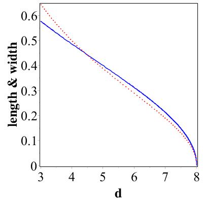
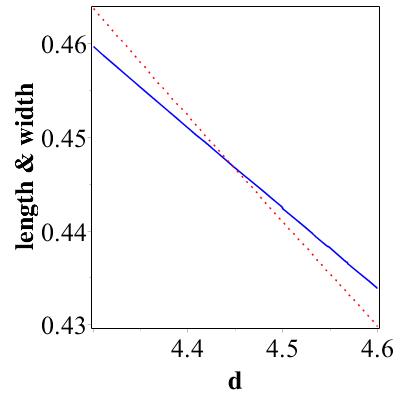
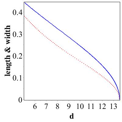
Figure 9. The minimum of length $d^{{}^{\prime}}_{LKE_{min}}$ (red,dot) and the maximum of width $d^{{}^{\prime}}_{WKE_{max}}$(blue,solid) of the contour line above the critical height $d_{c}$. In panels (a, b), $c=1$, the latter is the local picture of the former, and the crossing point is given at $d=4.444$. In panel (c), at $c=1.3$, there is no crossing point.

For $\beta\not=\frac{a}{2c^{2}}$, we do not analyse this condition $d^{{}^{\prime}}_{LKE}=d^{{}^{\prime}}_{WKE}$ because of its complexity, and then Figure 10 is plotted to merely show the evolution of three localization characters on $d$. In order to show the existence of $d^{{}^{\prime}}_{LKE}\not=d^{{}^{\prime}}_{WKE}$, Figure 11 is plotted for this case.

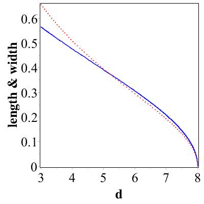
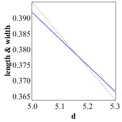
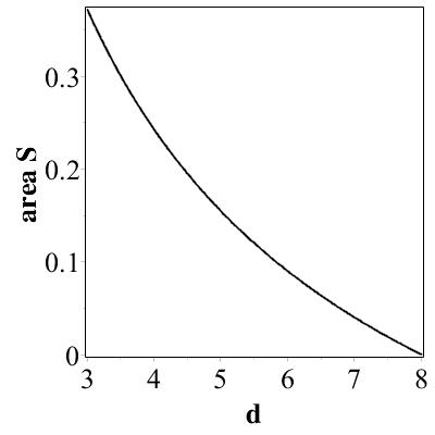
Figure 10. The length $d_{LKE}$ (red,dot) and width $d_{WKE}$(blue,solid) and the area $S$ of the contour line above the critical height $d_{c}$ with parameters $a=1/2,c=1,\beta=0.30$. There is a crossing point at $d=5.163$ in panel (a), panel(b) is the local picture of panel(a).

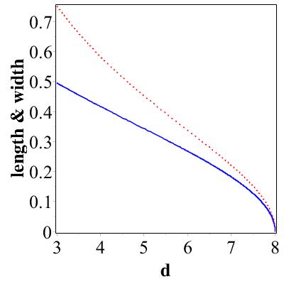
Figure 11. The length $d_{LKE}$ (red,dot) and width $d_{WKE}$(blue,solid) of the contour line above the critical height $d_{c}$ with parameters $a=1/2,c=1,\beta=0.40$. There is no crossing point.

From our above investigations, it is clear that by suitably manipulating the value of “$d$”, one can choose suitable area, length, width and amplitude of the rogue wave type optical pulses. To the best our knowledge, so far only variable coefficients of the nonlinear evolution equations have been used to manipulate the optical rogue waves. By suitably correlating the value of $d$ in terms of the experimental parameter, our results may be useful for the experimental realization of the control of the rogue wave. Moreover, the area $S$ and extreme values of length and width are independent of $\beta$, which means that higher-order terms in the KE equation do not have contribution of these three localization characters.

5. Conclusions

In this paper, we use the contour line method to study the localization characters of the first-order RW solution $|u_{rw}^{[1]}|^{2}$ of the KE equation. A full evolution process for the contour line with height $c^{2}+d$ along the orthogonal direction of the ($t,x$)-plane of the RW $|u_{rw}^{[1]}|^{2}$ can be summarized as follows: A point at height $9c^{2}$ generates a convex curve for $3c^{2}\leq d<8c^{2}$, whereas it becomes a concave curve for $0<d<3c^{2}$, next it reduces to a hyperbola on asymptotic plane (i.e. equivalently $d=0$), and the two branches of the hyperbola become two separate convex curves when $-c^{2}<d<0$, and finally they reduce to two separate points at $d=-c^{2}$.

Analytical formulas of length, width and area of the RW $|u_{rw}^{[1]}|^{2}$ with height $d(8c^{2}>d>0)$ are discussed according to two cases: $3c^{2}>d>0$ (below the critical value $d_{c}$) and $8c^{2}>d\geq 3c^{2}$ (above the critical value $d_{c}$). All of them are monotonically decreasing functions of $d$. In the above-mentioned three characters, only length for two cases has a same formula, and length and width are equal for some special values of $d$ and $c$. Under condition $\beta=\frac{a}{2c^{2}}$, the length reaches its minimum, but width gives a maximum. The main differences of two cases are listed by:

• Contour line is concave for the former, but convex for the latter. The critical value of height for the turning between convex and concave profile is $d_{c}=3c^{2}$.

• Different formulas for width.

• Different formulas for area.

• Different intervals of $c$ to get equal extreme values of length and width: $c\in(\frac{\sqrt{5}}{2},\sqrt{2})$ for former, but $c\in(\frac{\sqrt{3}}{2},\frac{\sqrt{5}}{2}]$ for the latter.

Our in-depth analysis on the contour line will be useful for experimentalist to control the patterns of the rogue wave ultra-short optical light pulses.

Since the KE is equivalent to the NLS by a nonlinear transformation $q=u\exp(2i\beta\int|u|^{2}dx)$ [7] regarding a solution $u$ of the former and a solution $q$ of the latter, in order to show the true characteristics of the KE equation, it is also interesting and necessary to study the phase of the first-order rogue wave $u^{[1]}_{rw}$ of the KE. This has been done partially by studying the real part of the first-order RW Re$u^{[1]}_{rw}$ in Ref.[23], which has shown that Re$u^{[1]}_{rw}$ has a central pattern around point ($0,0$) and alternately appeared parallels (see Figure 3 in Ref.[23]). This observation implies clearly that Re$u^{[1]}_{rw}$ is nonlocal. Thus, it is more essential to study the localized property of a phase difference $\Delta\theta=2\beta\int|u|^{2}dx$ [23] between above two solutions. Substituting $u=u^{[1]}_{rw}$ into $\Delta\theta$, it becomes

$$\Delta\theta= 2\beta c^{2}x+\frac{32c^{2}\beta t(2\beta c^{2}-a)+16c^{2}\beta x}{16c^{2}t(x+c^{2}t)(2\beta c^{2}-a)^{2}+4c^{2}x^{2}+16c^{4}t^{2}+1},$$

which is plotted in Figure 12( see also in Figure 4 of Ref.[23]). There exist a remarkable peak and hollow in the profile of $\Delta\theta$. If $t$ is large sufficiently, $\Delta\theta=2\beta c^{2}x$ which gives an asymptotic plane. So, in order to illustrate clearly the localized property of the $\Delta\theta$, it is better to study the contour lines of $\widetilde{\Delta\theta}=\Delta\theta-2\beta c^{2}x$ by removing the oblique asymptotic background, namely

$$\widetilde{\Delta\theta}=\frac{32c^{2}\beta t(2\beta c^{2}-a)+16c^{2}\beta x}{16c^{2}t(x+c^{2}t)(2\beta c^{2}-a)^{2}+4c^{2}x^{2}+16c^{4}t^{2}+1}.$$

$\widetilde{\Delta\theta}$ is plotted in Figures 13(a,b), which shows $\widetilde{\Delta\theta}$ is doubly localized in both $x$ and $t$. A simple calculation gives that $\widetilde{\Delta\theta}|_{max}=4\beta c$ at point ($t=0,x=\frac{1}{2c}$) and $\widetilde{\Delta\theta}|_{min}=-4\beta c$ at point ($t=0,x=-\frac{1}{2c}$), and the height of the asymptotic plane for $\widetilde{\Delta\theta}$ is zero. Setting $d\in[-4\beta c,4\beta c]$, an algebraic equation of the contour line at height $d$ is given by

$$256\,{c}^{6}d\left(4\,{\beta}^{2}{c}^{4}-4\,a\beta\,{c}^{2}+{a}^{2}+{c}^{2}\right)t^{4}+256c^{6}(a-\beta c^{2})(dx-2\beta)t^{3}+16\,{c}^{2}(4\,{\beta}^{2}{c}^{4}d$$

$$+4\,{c}^{4}d{x}^{2}-16\,\beta\,{c}^{4}x-4\,a\beta\,{c}^{2}d+{a}^{2}d+2\,{c}^{2}d)t^{2}+16c^{2}(a-\beta c^{2})(dx-2\beta)t+d=0.$$ (21)

In particular, the contour line is a straight line on asymptotic plane with height zero, namely $x=2(-2\beta c^{2}+a)t$. By a similar analysis of the contour line for $u^{[1]}_{rw}$ , we find a full evolution of the contour line of phase difference $\widetilde{\Delta\theta}$ as follows: A point at height $4\beta c$ generates a convex curve for $0<d<4\beta c$, next it reduces to a straight line on asymptotic plane (i.e. equivalently $d=0$), and then this straight line becomes a convex curve when $-4\beta c<d<0$, and finally it reduced to a point at $d=-4\beta c$, which is confirmed by Figure 13(c). Clearly, the evolution of contour line of $\widetilde{\Delta\theta}$ is different from the contour line of the $u^{[1]}_{rw}$.

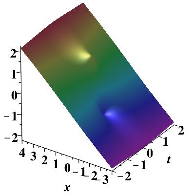
Figure 12. The phase difference $\Delta\theta$ between rogue wave solutions of the KE and NLS with parameters $a=1,c=1$ and $\beta=0.25$.

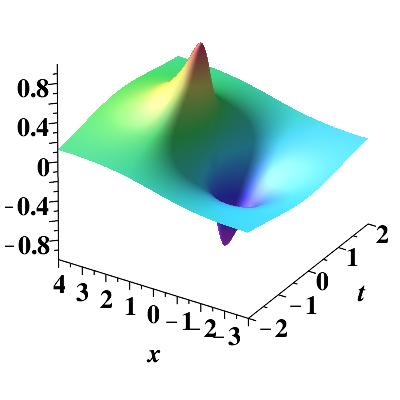
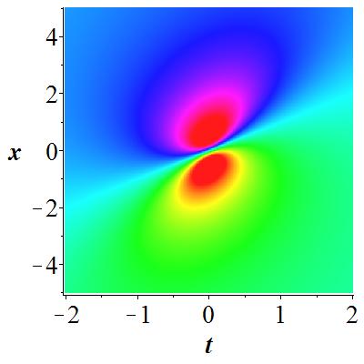
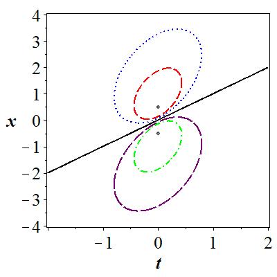
Figure 13. The phase difference $\widetilde{\Delta\theta}$ with parameters $a=1,c=1$ and $\beta=0.25$. Panel (b) is the density plot of (a). Panel (c) is plotted for the contour lines at different heights of (a). In panel (c), the straight line (solid black) is plotted for $d=0$. In upper plane of (c) devided by the straight line, different values of $d$ from outside to inside: d=0.5(red dot),0.3(blue dash). In lower plane of (c), different values of $d$ from outside to inside: d=-0.3 (purple long dash), -0.5 (green dash dot). The point in upper plane is the maximum attained at $d=4\beta c=1$, but the point in lower plane is the minimum attained at $d=-4\beta c=-1$.

Acknowledgments This work is supported by the NSF of China under Grant No.11271210 and K.C. Wong Magna Fund in Ningbo University. J. He thanks sincerely Prof. A.S. Fokas for arranging the visit to Cambridge University in 2012-2015 and for many useful discussions. K.P. thanks the DST,NBHM, IFCPAR,DST-FCT and CSIR, Government of India, for the financial support through major projects. We thank referees for their helpful suggestions on the early version of this paper.

Appendix

In this appendix, a few additional explanations about the contour line below the asymptotic background will be given. For this case, the height of the contour line is $c^{2}-d$ ($0<d<c^{2}$) along the orthogonal direction of the ($t,x$)-plane, which is a closed curve defined by Eq.(4) with $-d$ instead of $d$, i.e.

$$16c^{4}dx^{4}+(256\beta c^{6}d-128ac^{4}d)tx^{3}+S_{1}x^{2}+S_{2}x+S_{3}t^{4}+S_{4}t^{2}+8c^{2}+d=0,$$ (22)

where

$$S_{1}= \left(1536\,{\beta}^{2}{c}^{8}d-1536\,a\beta\,{c}^{6}d+384\,{a}^{2}{c}^{4}d+128\,{c}^{6}d\right){t}^{2}-32\,{c}^{4}+8\,{c}^{2}d,$$

$$S_{2}= 4096\,{\beta}^{3}{c}^{10}d-6144\,a{\beta}^{2}{c}^{8}d+3072\,{a}^{2}\beta\,{c}^{6}d+1024\,\beta\,{c}^{8}d-512\,{a}^{3}{c}^{4}d-512\,a{c}^{6}d,$$

$$S_{3}= 4096\,{\beta}^{4}{c}^{12}d-8192\,a{\beta}^{3}{c}^{10}d+6144\,{a}^{2}{\beta}^{2}{c}^{8}d+2048\,{\beta}^{2}{c}^{10}d$$

$$-2048\,{a}^{3}\beta\,{c}^{6}d-2048\,a\beta\,{c}^{8}d+256\,{a}^{4}{c}^{4}d+512\,{a}^{2}{c}^{6}d+256\,{c}^{8}d,$$

$$S_{4}= -512\,{\beta}^{2}{c}^{8}+128\,{\beta}^{2}{c}^{6}d+512\,a\beta\,{c}^{6}-128\,a\beta\,{c}^{4}d-128\,{a}^{2}{c}^{4}-128\,{c}^{6}-32\,{a}^{2}{c}^{2}d+32\,{c}^{4}d.$$

Actually, Eq. (22) can be expressed explicitly by the following four branches

$$l_{01}: x=-4\beta c^{2}t+2at+\frac{G_{1}}{2dc},\,\,l_{02}:x=-4\beta c^{2}t+2at-\frac{G_{1}}{2dc},$$ (23)

$$l_{03}: x=-4\beta c^{2}t+2at+\frac{G_{2}}{2dc},\,\,l_{04}:x=-4\beta c^{2}t+2at-\frac{G_{2}}{2dc},$$ (24)

in which

$$G_{1}=\sqrt{-16c^{4}d^{2}t^{2}+4c^{2}d-d^{2}+4cd\sqrt{-16c^{4}dt^{2}+c^{2}-d}},$$

$$G_{2}=\sqrt{-16c^{4}d^{2}t^{2}+4c^{2}d-d^{2}-4cd\sqrt{-16c^{4}dt^{2}+c^{2}-d}}.$$

and $t\in[-\frac{\sqrt{d(c^{2}-d)}}{4dc^{2}},\frac{\sqrt{d(c^{2}-d)}}{4dc^{2}}]$. Set $G_{A}=-16c^{4}d^{2}t^{2}+4c^{2}d-d^{2},G_{B}=4cd\sqrt{-16c^{4}dt^{2}+c^{2}-d},G_{1}=\sqrt{G_{A}+G_{B}},\,G_{2}=\sqrt{G_{A}-G_{B}}$ and $y=t^{2}$, then $G_{A}>0$ and $G_{B}>0$ when $t\in(-\frac{\sqrt{d(c^{2}-d)}}{4dc^{2}},\frac{\sqrt{d(c^{2}-d)}}{4dc^{2}})$, and $G_{A}^{2}-G_{B}^{2}={d}^{3}\left(16\,{c}^{4}y+1\right)\left(16\,{c}^{4}dy+8\,{c}^{2}+d\right)\geq 0$. Thus $G_{A}-G_{B}>0$ when $t\in(-\frac{\sqrt{d(c^{2}-d)}}{4dc^{2}},\frac{\sqrt{d(c^{2}-d)}}{4dc^{2}})$, which implies $G_{1}$ and $G_{2}$ are real functions of $t$. According to the four branches, four end points are represented explicitly by

$$P_{1}^{{}^{\prime}}=(\frac{\sqrt{d(c^{2}-d)}}{4c^{2}d},\frac{(a-2\beta c^{2})\sqrt{d(c^{2}-d)}+c^{2}\sqrt{3d}}{2c^{2}d}),$$

$$P_{2}^{{}^{\prime}}=(-\frac{\sqrt{d(c^{2}-d)}}{4c^{2}d},-\frac{(a-2\beta c^{2})\sqrt{d(c^{2}-d)}-c^{2}\sqrt{3d}}{2c^{2}d}),$$

$$P_{1}^{{}^{\prime\prime}}=(\frac{\sqrt{d(c^{2}-d)}}{4c^{2}d},\frac{(a-2\beta c^{2})\sqrt{d(c^{2}-d)}-c^{2}\sqrt{3d}}{2c^{2}d}),$$

$$P_{2}^{{}^{\prime\prime}}=(-\frac{\sqrt{d(c^{2}-d)}}{4c^{2}d},-\frac{(a-2\beta c^{2})\sqrt{d(c^{2}-d)}+c^{2}\sqrt{3d}}{2c^{2}d}).$$

Now we will prove that the contour line below the asymptotic background is always convex. The derivatives with respect to t of the four branches are

$$-4\beta c^{2}+2a+\frac{G_{3}}{G_{1}}-x^{\prime}(t)=0,\,\,-4\beta c^{2}+2a+\frac{G_{3}}{G_{1}}-x^{\prime}(t)=0,$$ (25)

$$-4\beta c^{2}+2a+\frac{G_{4}}{G_{2}}-x^{\prime}(t)=0,\,\,-4\beta c^{2}+2a+\frac{G_{4}}{G_{2}}-x^{\prime}(t)=0,$$ (26)

where $G_{3}=-8c^{3}dt-\frac{16c^{4}dt}{\sqrt{-16c^{4}dt^{2}+c^{2}-d}}$,$G_{4}=-8c^{3}dt+\frac{16c^{4}dt}{\sqrt{-16c^{4}dt^{2}+c^{2}-d}}$. In order to find a convex point on the contour line, we set $x^{\prime}(t)=k$ in Eqs. (25,26), and then get four equivalent equations of $t$ as follows

$$-8c^{3}dt(2c+\sqrt{-16c^{4}dt^{2}+c^{2}-d})=0,\,\,8c^{3}dt(2c+\sqrt{-16c^{4}dt^{2}+c^{2}-d})=0,$$ (27)

$$8c^{3}dt(2c-\sqrt{-16c^{4}dt^{2}+c^{2}-d})=0,\,\,-8c^{3}dt(2c-\sqrt{-16c^{4}dt^{2}+c^{2}-d})=0.$$ (28)

Solving above Eqs. (27,28), we find only one real solution $t=0$, which means that contour line below the asymptotic background is always convex for $0<d<c^{2}$.

References

[1]R.Y. Chiao, E. Garmire and C.H. Townes,1964, Self-trapping of optical beams, Phys.Rev. Lett. 13, 479–482.
[2] V. E. Zakharov, 1968, Stability of perodic waves of finite amplitude on the surface of a deep fluid,
J.Appl.Mech. Tech. Phys. 9, 190–194.
[3] M.J. Ablowitz, and P.A. Clarkson, 1991, Solitons, Nonlinear Evolution Equations and Inverse Scattering (Cambridge University Press, Cambridge, UK).
[4] N. Akhmediev, A. Ankiewicz, 1997, Solitons: Nonlinear pulses and beams (Chapman & Hall, London).
[5]A. Hasegawa, M. Matsumoto, 2010, Optical Solitons in Fibers (Springer, Berlin).
[7] A. Kundu, 1984, Landau-Lifshitz and higher-order nonlinear systems gauge generated from nonlinear Schrödinger-type equations, J. Math. Phys. 25 3433-3438.
[8]F. Calogero, W. Eckhaus, 1987, Nonlinear evolution equations, rescalings, model PDEs and their integrability. I,
Inverse Problems 3, 229-262.
[9]Y.J. Xiang, X.Y.Dai, S.C. Wen, J.Guo and D.Y. Fan, 2011, Controllable Raman soliton self-frequency shift in
nonlinear metamaterials, Phys.Rev. A 84, 033815.
[10] R. Radhakrishnan, A. Kundu, and M. Lakshmanan, 1999,Coupled nonlinear Schrödinger equations with cubic-quintic nonlinearity: Integrability and soliton interaction in non-Kerr media, Phys. Rev. E 60, 3314-3323.
[11] A. Choudhuri, K.Porsezian, 2012, Dark-in-the-Bright solitary wave solution of higher-order nonlinear Schrödinger
equation with non-Kerr terms, Opt. Commun. 285, 364-367.
[12] A. Choudhuri, K.Porsezian, 2012, Impact of dispersion and non-Kerr nonlinearity on the modulational instability
of the higher-order nonlinear Schrödinger equation, Phys. Rev. A 85, 033820.
[13] A. Choudhuri, K.Porsezian, 2013, Higher-order nonlinear Schrödinger equation with derivative non-Kerr nonlinear terms:
A model for sub-10-fs-pulse propagation, Phys.Rev.A 88, 033808.
[14] R.S.Johnson, 1977, On the modulation of water waves in the neighbourhood of , Proc.Roy.Soc.
London Ser.A,357, 131-141.
[15] P. A. Clarkson, C. M. Cosgrove, 1987, Painlevé analysis of the nonlinear Schrödinger family of equations,
J. Phys. A: Math. Gen. 20, 2003-2024.
[16]X. G. Geng, 1992, A hierarchy of nonlinear evolution equations, its Hamiltonian structure and classical integrable
system, Physica A 80, 241-251.
[17]X. G. Geng and H. W. Tam, 1999, Darboux transformation and soliton solutions for generalized nonlinear Schrödinger equations,
J. Phys. Soc. Jpn. 68, 1508-1512.
[18]S. Kakei, N. Sasa and J. Satsuma, 1995, Bilinearization of a generalized derivative nonlinear Schrödinger equation,
J. Phys. Soc. Jpn. 64, 1519-1523.
[19]Z. Feng and X. Wang, 2001, Explicit exact solitary wave solutions for the Kundu equation and the derivative
Schrödinger equation, Phys. Scripta 64, 7-14.
[20] A. Kundu, 2006, Integrable Hierarchy of Higher Nonlinear Schrödinger Type Equations, Symmetry, Integrability and Geometry: Methods and Applications 2, No. 78.
[21]X. Lü, M. S. Peng, 2013, Systematic construction of infinitely many conservation laws
for certain nonlinear evolution equations in mathematical
physics, Commun. Nonlinear Sci. Numer. Simulat. 18, 2304-2312.
[22]Q. L. Zha, 2013, On Nth-order rogue wave solution to the generalized nonlinear
Schrödinger equation, Phys. Lett. A 377, 855-859.
[23] D. Q. Qiu, J. S. He, Y. S. Zhang, and K. Porsezian, 2015, Darboux Transformation of the Kundu-Eckhaus equation,
Proc. R. Soc. A 471, 20150236.
[24] X. Wang, B. Yang, Y Chen, and Y. Q. Yang, 2014, Higher-order rogue wave solutions of the Kundu-Eckhuas equation, Phys. Scr. 89. 095210.
[25] C. Garrett, J. Gemmrich, 2009, Rogue waves, Phys. Today 62, 62-63.
[26] C. Kharif, E. Pelinovsky, and A. Slunyaev, 2009, Rogue Waves in the Ocean (Springer, Heidelberg).
[27]A. R. Osborne, 2010, Nonlinear ocean waves and the inverse scattering transform (Academic Press, New York).
[28]D. R. Solli, C. Ropers, P. Koonath and B. Jalali, 2007, Optical rogue waves, Nature 450, 1054-1057.
[29]B. Kibler, J. Fatome, C. Finot, G. Millot, F. Dias, G. Genty, N. Akhmediev and J. M. Dudley, 2010, The
Peregrine soliton in nonlinear fibre optics, Nat. Phys. 6, 790–795.
[30]A. Chabchoub, N. P. Hoffmann and N. Akhmediev, Rogue wave observation in a water wave tank, 2011, Phys. Rev. Lett. 106, 204502.
[31] M. Shats, H. Punzmann, and H. Xia, 2010, Capillary rogue waves, Phys. Rev. Lett. 104 104503.
[32] V. B. Efimov, A. N. Ganshin, G. V. Kolmakov, P. V. E. McClintock, and L. P. Mezhov-Deglin, 2010, Rogue waves in superfluid helium, Eur. Phys. J. Spec. Top 185, 181-193.
[33] Y. V. Bludov, V. V. Konotop, and N. Akhmediev, 2009, Matter rogue waves, Phys. Rev. A 80, 033610.
[34] W. M. Moslem, P. K. Shukla, and B. Eliasson, 2011, Surface plasma rogue waves, Euro. Phys. Lett 96, 25002.
[35] L. Stenflo, M. Marklund, 2010, Rogue waves in the atmosphere, J. Plasma Phys. 76, 293-295.
[36] J. S. He, L. H. Wang, L. J. Li, K. Porsezian, and R. Erd lyi, 2014, Few-cycle optical rogue waves: Complex modified Korteweg-de Vries equation, Phys. Rev. E 89, 062917.
[37] Y. S. Zhang, L. J. Guo, A. Chabchoub, and J. S. He, 2014, The darboux transfourmation and higher-order rogue wave modes for a derivative nonliner Schrödinger equation, arxiv: 1409. 7923v1.
[38] D.Q.Qiu, Y.S.Zhang, J.S.He, 2016, The rogue wave solutions of a new (2+1)-dimensional equation,
Commun. Nonlinear Sci. Numer. Simulat. 30, 307-315.