Isoptic surfaces of polyhedra

Abstract

The theory of the isoptic curves is widely studied in the Euclidean plane $\mathbf{E}^{2}$ (see [2] and [20] and the references given there). The analogous question was investigated by the authors in the hyperbolic $\mathbf{H}^{2}$ and elliptic $\mathcal{E}^{2}$ planes (see [4], [5], [8]), but in the higher dimensional spaces there are only a few result in this topic.

In [7] we gave a natural extension of the notion of the isoptic curves to the $n$-dimensional Euclidean space $\mathbf{E}^{n}$ $(n\geq 3)$ which are called isoptic hypersurfaces. Now we develope an algorithm to determine the isoptic surface $\mathcal{H}_{\mathcal{P}}$ of a $3$-dimensional polytop $\mathcal{P}$.

We will determine the isoptic surfaces for Platonic solids and for some semi-regular Archimedean polytopes and visualize them with Wolfram Mathematica.

1 Introduction

Let $G$ be one of the constant curvature plane geometries, either the Euclidean $\mathbf{E}^{2}$ or the hyperbolic $\mathbf{H}^{2}$ or the elliptic $\mathcal{E}^{2}$. The isoptic curve of a given plane curve $\mathcal{C}$ is the locus of points $P\in G$ where $\mathcal{C}$ is seen under a given fixed angle $\alpha$ $(0<\alpha<\pi)$. An isoptic curve formed by the locus of tangents meeting at right angles is called orthoptic curve. The name isoptic curve was suggested by Taylor in [19].

In [2] and [3] the isoptic curves of the closed, strictly convex curves are studied, using their support function. The papers [21] and [22] deal with curves having a circle or an ellipse for an isoptic curve. Further curves appearing as isoptic curves are well studied in the Euclidean plane geometry $\mathbf{E}^{2}$, see e.g. [15], [20]. Isoptic curves of conic sections have been studied in [10] and [18]. A lot of papers concentrate on the properties of the isoptics e.g. [16], [17], and the reference given there. The papers [13] and [14] deal with inverse problems.

In the hyperbolic and elliptic planes $\mathbf{H}^{2}$ and $\mathcal{E}^{2}$ the isoptic curves of segments and proper conic sections are determined by the authors ([4], [5], [6]). In [8] we extended the notion of the isoptic curves to the outer (non-proper) points of the hyperbolic plane and determined the isoptic curves of the generalized conic sections.

It is known, that the angle of two half-lines with vertex $A$ in the plane can be measured by the arc length on the unit circle around the point $A$. This statement can be generalized to the higher dimensional Euclidean spaces. The notion of the solid angle is well known and widely studied in the literatur (see [9]). We recall this definition concerning the $3$-dimensional Euclidean space $\mathbf{E}^{3}$ and we will apply it in the following.

Definition 1.1

The solid angle $\Omega_{S}(\mathbf{p})$ subtended by a surface $S$ is defined as the surface area of a unit sphere covered by the surface’s projection onto the sphere around $P(\mathbf{p})$.

Solid angle is measured in steradians, e.g. the solid angle corresponding to all of space being subtended is $4\pi$ steradians. Moreover, this notion has several important applications in physics (particular in astrophysics, radiometry or photometry) (see [1]) even in computational geometry (see [11]) and we will use it for the definition of the isoptic surfaces.

The isoptic hypersurface in the $n$-dimensional Euclidean space $(n\geq 3)$ is defined in [7] and now, we recall some statements and specify them to the $\mathbf{E}^{3}$.

Definition 1.2

The isoptic hypersurface $\mathcal{H}_{\mathcal{D}}^{\alpha}$ in $\mathbf{E}^{3}$ of an arbitrary $3$-dimensional compact domain $\mathcal{D}$ is the locus of points $P$ where the measure of the projection of $\mathcal{D}$ onto the unit sphere around $P$ is a given fixed value $\alpha$ $(0<\alpha<2\pi)$ (see Fig. 1).

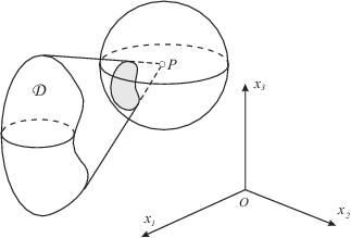
Figure 1: Projection of a compact domain $\mathcal{D}$ to unit sphere in $\mathbf{E}^{3}$

In this paper we develope an algorithm and the corresponding computer program to determine the isoptic surface of an arbitrary convex polyhedron in the $3$-dimensional Euclidean space. We apply this algorithm for the regular Platonic solids and some semi-regular Archimedean solids as well. This generalization of the isoptic curves to the $3$-dimensional space provide several new way to extend the notion of isoptic surfaces to the ”smooth surfaces” and for applications.

2 The algorithm

In this section we discuss the algorithm developed to determine the isoptic surface of a given polyhedron.

1. We assume that an arbitrary polyhedron $\mathcal{P}$ is given by the usual data structure. This consists of the list of facets $\mathcal{F}_{\mathcal{P}}$ with the set of vertices $V_{i}$ in clockwise order. Each facet can be embedded into a plane.

   It is well known, that if $\mathbf{a}\in\mathbf{R}^{3}\setminus\{\mathbf{0}\}$ and $b\in\mathbf{R}$ then $\{\mathbf{x}\in\mathbf{R}^{3}|\mathbf{a}^{T}\mathbf{x}=b\}$ is a plane and $\{\mathbf{x}\in\mathbf{R}^{3}|\mathbf{a}^{T}\mathbf{x}\leq b\}$ define a halfspace. Every polyhedron is the intersection of finitely many halfspaces. Therefore an arbitrary polyhedron can also be given by a system of inequality $A\mathbf{x}\leq\mathbf{b}$ where $A\in\mathbf{R}^{m\times 3}$ ($4\leq m\in\mathbb{N}$), $\mathbf{x}\in\mathbf{R}^{3}$ and $\mathbf{b}\in\mathbf{R}^{m}$. The solution set of the above equation system provide the polyhedron.

2. We have to decide for an arbitrary point $P(\mathbf{p})\in\mathbf{E}^{3}$, that which faces of $\mathcal{P}$ ”can be seen” from it. Let us denote the $i^{\mathrm{th}}$ facet of $\mathcal{P}$ with $\mathcal{F}_{\mathcal{P}}^{i}$ $(i=1\dots m)$ and $\mathbf{a}^{i}$ is the vector derived by $i^{\mathrm{th}}$ row of the matrix $A$ which characterize the face $\mathcal{F}_{\mathcal{P}}^{i}$.

   Since the polyhedron $\mathcal{P}$ is given by the inequality system ${A}\mathbf{x}\leq\mathbf{b}$, where all inequality ${\mathbf{a}^{i}}\mathbf{x}\leq b_{i}$ ($i\in\{1,2\dots,m\}$) is assigned to a certain face, therefore the facet $\mathcal{F}_{\mathcal{P}}^{i}$ is visible from $P$ iff the inequality $\mathbf{a}^{i}\mathbf{p}>{b_{i}}$ holds.

   Now, we define the characteristic function $\mathbb{I}^{i}_{\mathcal{P}}(\mathbf{x})$ for each face $\mathcal{F}_{\mathcal{P}}^{i}$:

   $$\mathbb{I}^{i}_{\mathcal{P}}(\mathbf{x})=\left\{\begin{array}[]{lr}1&\mathbf{a}^{i}\mathbf{x}>{b_{i}}\\ 0&\mathbf{a}^{i}\mathbf{x}\leq{b_{i}}\end{array}\right.$$

3. Using the Definition 1.1, let $\Omega_{i}(\mathbf{p}):=\Omega_{\mathcal{F}^{i}_{\mathcal{P}}}(\mathbf{p})$ be the solid angle of the facet $\mathcal{F}_{\mathcal{P}}^{i}$ regarding the point $P(\mathbf{p})$.

   To determine $\Omega_{i}(\mathbf{p})$, we use the machinery of the spherical geometry. Let us suppose that $\mathcal{F}_{\mathcal{P}}^{i}$ contains $n_{i}$ vertices, $V_{i_{j}}(\mathbf{x}_{i_{j}})$, $(j=1\dots n_{i})$ where the vertices are given in clockwise order. Projecting these vertexes onto the unit sphere around $P(\mathbf{p})$ we get a spherical $n_{i}$-gon (see Fig 2)

   

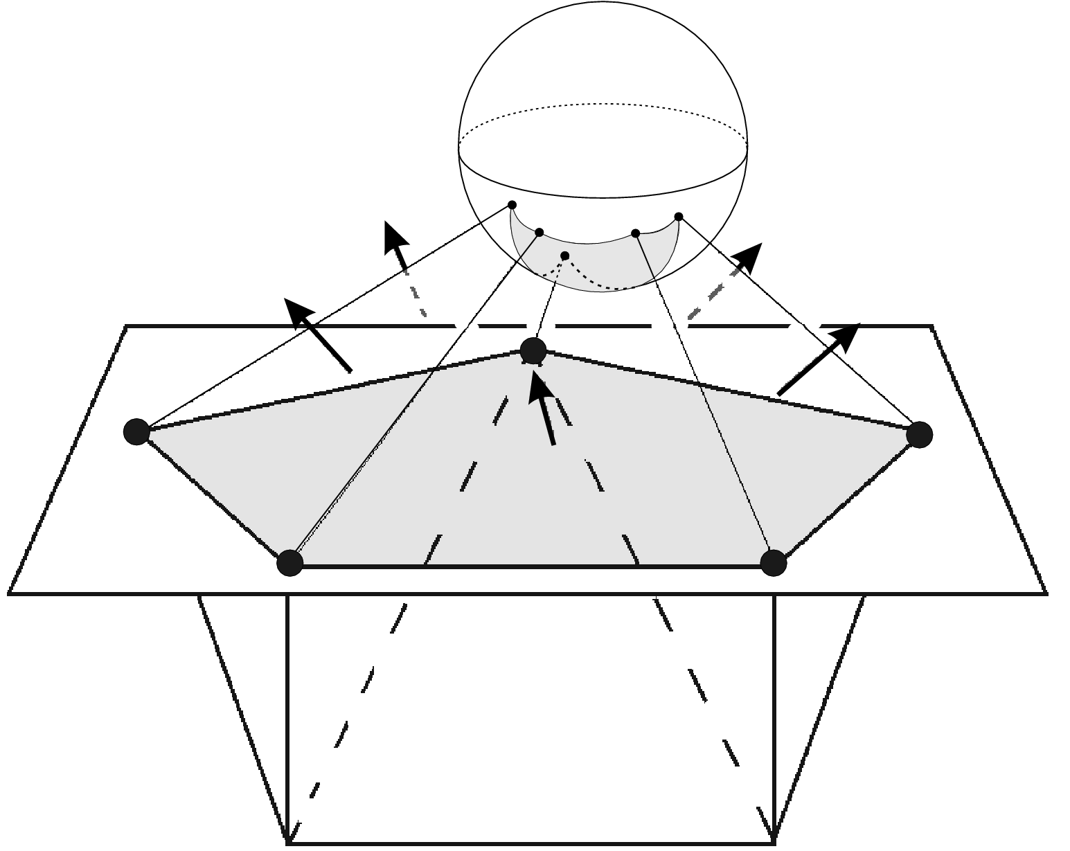
   Figure 2: Projection of a compact domain $\mathcal{D}$ to unit sphere in $\mathbf{E}^{3}$

   whose area can be calculated by the usual formula

   $$\Omega_{i}(\mathbf{p})=(\Theta-(n_{i}-2)\pi).$$

   Here $\Theta$ is the sum of the angles $\tau_{j}$ of the spherical polygon $\mathcal{F}_{\mathcal{P}}^{i}$ where the angles are measured in radians.

4. To obtain these $\tau_{j}$ angles, we need to determine the angles of the planes that contain the neigbouring edges $\overline{PV}_{i_{k}}$ where $k=j-1,j$ and $k=j,j+1$:

   $$\tau_{j}=\pi-\arccos\left(\frac{\left\langle\overrightarrow{PV}_{i_{j-1}}\times\overrightarrow{PV}_{i_{j}},\overrightarrow{PV}_{i_{j}}\times\overrightarrow{PV}_{i_{j+1}}\right\rangle}{\left|\overrightarrow{PV}_{i_{j-1}}\times\overrightarrow{PV}_{i_{j}}\right|\left|\overrightarrow{PV}_{i_{j}}\times\overrightarrow{PV}_{i_{j+1}}\right|}\right).$$

   Finally, we get the solid angle function $\Omega_{i}(\mathbf{x})$ of the facet $\mathcal{F}_{\mathcal{P}}^{i}$ for any $\mathbf{x}\in\mathbf{R}^{3}:$

   $$\Omega_{i}(\mathbf{x})=2\pi-\sum_{j=1}^{n_{i}}\arccos\left(\frac{\left\langle\overrightarrow{XV}_{i_{j-1}}\times\overrightarrow{XV}_{i_{j}},\overrightarrow{XV}_{i_{j}}\times\overrightarrow{XV}_{i_{j+1}}\right\rangle}{\left|\overrightarrow{XV}_{i_{j-1}}\times\overrightarrow{XV}_{i_{j}}\right|\left|\overrightarrow{XV}_{i_{j}}\times\overrightarrow{XV}_{i_{j+1}}\right|}\right),$$

5. We can summarize our results in the following

   Theorem 2.1

   Let us given a solid angle $\alpha$ ($0<\alpha<2\pi$) and a convex polyhedron $\mathcal{P}$ by its data structure and its set of inequality. Then its isoptic surface can be determined by the equation

   $$\alpha=\sum_{i=1}^{m}\mathbb{I}^{i}_{\mathcal{P}}(\mathbf{x})\Omega_{i}(\mathbf{x}).$$

The results and computations will be demonstrated in the following subsection through the computation related to the regular tetrahedron and along with some figures.

Remark 2.2

1. The algorithm can be easily extended for non-closed directed surfaces e. g. for subdivision surfaces.

2. If we have a convex polyhedron, than projecting its whole surface to the unit sphere, we obtain a double coverage (double solid angle) of the given polyhedron, therefore the algorithm can be changed i.e. it is not necessary to determine the visible faces. In this case the isoptic surfaces are determined by the following implicit equation:

   $$\alpha=\frac{1}{2}\sum_{i=1}^{m}\Omega_{i}(\mathbf{x}).$$

2.1 Computations of the isoptic surface of a given regular tetrahedron

Following the steps of the above described algorithm, we will calculate the compound isoptic surface of a given regular tetrahedron $\mathcal{T}$ whose data structure is determined by its vertices and faces where the faces $\mathcal{F}_{\mathcal{P}}^{i}$ are given by their clockwise ordered vertices:

$$\begin{gathered}A_{1}=\left(0,0,\sqrt{\frac{2}{3}}-\frac{1}{2\sqrt{6}}\right),A_{2}=\left(-\frac{1}{2\sqrt{3}},-\frac{1}{2},-\frac{1}{2\sqrt{6}}\right),\\ A_{3}=\left(-\frac{1}{2\sqrt{3}},\frac{1}{2},-\frac{1}{2\sqrt{6}}\right),A_{4}=\left(\frac{1}{\sqrt{3}},0,-\frac{1}{2\sqrt{6}}\right),\\ \left\{\mathcal{F}_{\mathcal{T}}^{1},\left\{A_{2},A_{3},A_{4}\right\}\right\},\left\{\mathcal{F}_{\mathcal{T}}^{2},\left\{A_{3},A_{2},A_{1}\right\}\right\},\\ \left\{\mathcal{F}_{\mathcal{T}}^{3},\left\{A_{4},A_{1},A_{2}\right\}\right\},\left\{\mathcal{F}_{\mathcal{T}}^{4},\left\{A_{1},A_{4},A_{3}\right\}\right\}.\end{gathered}$$

The tetrahedron is also given by its system of inequality:

$$\left(\begin{array}[]{ccc}0&0&-4\sqrt{3}\\ -8\sqrt{6}&0&4\sqrt{3}\\ 4\sqrt{6}&-12\sqrt{3}&4\sqrt{3}\\ 4\sqrt{6}&12\sqrt{3}&4\sqrt{3}\end{array}\right)\left(\begin{array}[]{c}x\\ y\\ z\end{array}\right)\leq\left(\begin{array}[]{c}\sqrt{2}\\ 3\sqrt{2}\\ 3\sqrt{2}\\ 3\sqrt{2}\end{array}\right).$$

Since the final formula of the isoptic surface is too long to appear in print even for this simple example, we choose $i=1$ and derive only $\mathbb{I}^{1}_{\mathcal{P}}(\mathbf{x})$.

$$\mathbb{I}^{1}_{\mathcal{P}}(x,y,z)=\left\{\begin{array}[]{lr}1&-4\sqrt{3}z>\sqrt{2}\\ 0&-4\sqrt{3}z\leq\sqrt{2}\end{array}\right..$$

For the resulted surface, see Fig. 3. (left), and in Fig. 3. (right) we describe a part of the tetrahedral isoptic surface of angle $\alpha=\pi/8$. The surface $\phi_{1,2}$ is derived by the solid angles belonging to the faces $\mathcal{F}_{\mathcal{T}}^{3}$ and $\mathcal{F}_{\mathcal{T}}^{4}$. The isoptic surface $\phi_{1}$ is derived by the solid angles belonging to the faces $\mathcal{F}_{\mathcal{T}}^{2}$, $\mathcal{F}_{\mathcal{T}}^{3}$ and $\mathcal{F}_{\mathcal{T}}^{4}$ and The isoptik surface $\phi_{2}$ is derived by the solid angles belonging to the faces $\mathcal{F}_{\mathcal{T}}^{1}$, $\mathcal{F}_{\mathcal{T}}^{3}$ and $\mathcal{F}_{\mathcal{T}}^{4}$.

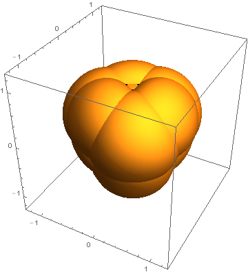
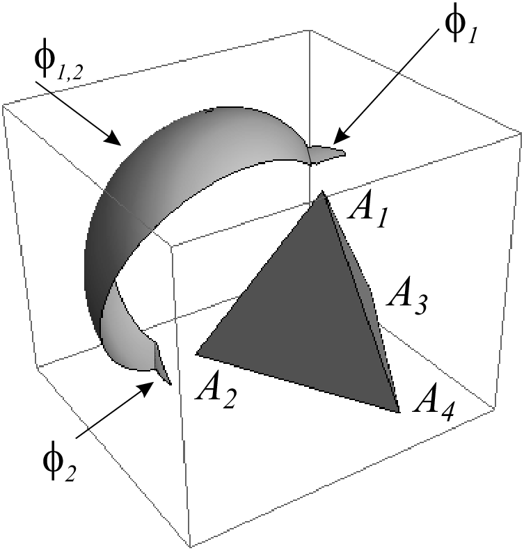
Figure 3: Isoptic surface of the regular tetrahedron for $\alpha=\pi/8$. A part of the tetrahedral isoptic surface e.g. The surface $\phi_{1,2}$ is derived by the solid angles belonging to the faces $\mathcal{F}_{\mathcal{T}}^{3}$ and $\mathcal{F}_{\mathcal{T}}^{4}$.

2.2 Isoptic surfaces to regular polyhedra and some Archimedean polyhedra

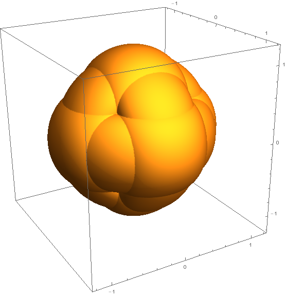
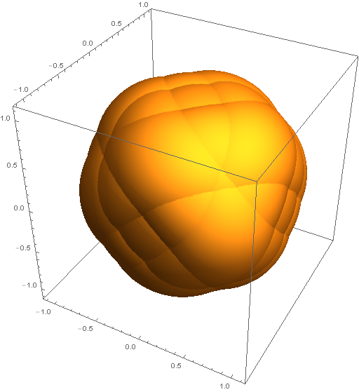
Figure 4: Isoptic surface of the cube $\alpha=\pi/2$ (left),
Isoptic surface of the regular octahedron for $\alpha=\pi/7$ (right)

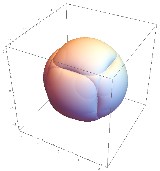
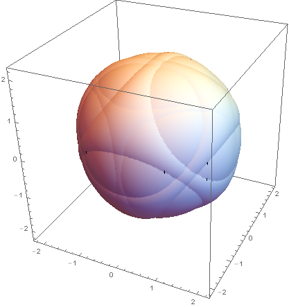
Figure 5: Isoptic surface of the truncated cube $\alpha=\pi$ (left)
Isoptic surface of the truncated octahedron $\alpha=2\pi/3$

References

- [1] Camp, D.C., Van Lehn, A.L.: Finite solid-angle corrections for Ge(Li) detectors, Nucl. Instrum. Methods, Vol. 76, No 2., (1969), 192-240.
- [2] Cieślak, W., Miernowski, A., Mozgawa, W. : Isoptics of a Closed Strictly Convex Curve, Lect. Notes in Math., 1481 (1991), pp. 28-35.
- [3] Cieślak, W., Miernowski, A., Mozgawa, W. : Isoptics of a Closed Strictly Convex Curve II, Rend. Semin. Mat. Univ. Padova 96, (1996), 37-49.
- [4] Csima, G., Szirmai, J.: Isoptic curves of the conic sections in the hyperbolic and elliptic plane, Stud. Univ. Žilina, Math. Ser. 24, No. 1, (2010), 15-22.
- [5] Csima, G., Szirmai, J.: Isoptic curves to parabolas in the hyperbolic plane, Pollac Periodica 7/1/1, (2012) 55-64.
- [6] Csima, G., Szirmai, J. : Isoptic curves of conic sections in constant curvature geometries, Mathematical Communications Vol 19/2,(2014) 277-290.
- [7] Csima, G., Szirmai, J. : On the isoptic hypersurfaces in the -dimensional Euclidean space, KoG (Scientific and professional journal of Croatian Society for Geometry and Graphics) 17, (2013) 53-57.
- [8] Csima, G., Szirmai, J. : Isoptic curves of generalized conic sections in the hyperbolic plane, Submitted manuscript (2015).
- [9] Gardner, R.P, Verghese, K.: On the solid angle subtended by a circular disc, Nucl. Instrum. Methods, Vol. 91, No 1., (1971), 163-167.
- [10] Holzmüller, G.: Einführung in die Theorie der isogonalen Verwandtschaft, B.G. Teuber, Leipzig-Berlin, 1882.
- [11] Joe, B.: Delaunay versus max-min solid angle triangulations for three-dimensional mesh generation, Int. J. Numer. Methods Eng., Vol 31, No. 5, (1991), 987-997.
- [12] Kunkli, R., Papp, I., Hoffmann, M.: Isoptics of Bézier curves, Computer Aided Geometric Design, 30, (2013), 78-84.
- [13] Kurusa, Á.: Is a convex plane body determined by an isoptic?, Beitr. Algebra Geom. 53/1, (2012), 281-294.
- [14] Kurusa, Á., Odor, T.: Isoptic characterization of spheres, J. Geom. 106/1, (2015) 63-73.
- [15] Loria, G. : Spezielle algebraische und traszendente ebene Kurve, 1 & 2, B.G. Teubner, Leipzig-Berlin, 1911.
- [16] Miernowski, A., Mozgawa, W. : On some geometric condition for convexity of isoptics, Rend. Semin. Mat., Torino 55, No.2 (1997), 93-98.
- [17] Michalska, M.: A sufficient condition for the convexity of the area of an isoptic curve of an oval, Rend. Semin. Mat. Univ. Padova 110, (2003), 161-169.
- [18] Siebeck, F. H.: Über eine Gattung von Curven vierten Grades, welche mit den elliptischen Funktionen zusammenhängen, J. Reine Angew. Math. 57 (1860), 359-370; 59 (1861), 173-184.
- [19] Taylor, C.: Note on a theory of orthoptic and isoptic loci., Proc. R. Soc. London XXXVIII (1884).
- [20] Wieleitener, H.: Spezielle ebene Kurven. Sammlung Schubert LVI, Göschen’sche Verlagshandlung. Leipzig, 1908.
- [21] Wunderlich, W.: Kurven mit isoptischem Kreis, Aequat. math. 6 (1971). 71-81.
- [22] Wunderlich, W.: Kurven mit isoptischer Ellipse, Monatsh. Math. 75 (1971) 346-362.