Gaussian state interferometry with passive and active elements

Abstract

We address precision of optical interferometers fed by Gaussian states and involving passive and/or active elements, such as beam splitters, photodetectors and optical parametric amplifiers. We first address the ultimate bounds to precision by discussing the behaviour of the quantum Fisher information. We then consider photodetection at the output and calculate the sensitivity of the interferometers taking into account the non unit quantum efficiency of the detectors. Our results show that in the ideal case of photon number detectors with unit quantum efficiency the best configuration is the symmetric one, namely, passive (active) interferometer with passive (active) detection stage: in this case one may achieve Heisenberg scaling of sensitivity by suitably optimizing over Gaussian states at the input. On the other hand, in the realistic case of detectors with non unit quantum efficiency, the performances of passive scheme are unavoidably degraded, whereas detectors involving optical parametric amplifiers allow to fully compensate the presence of loss in the detection stage, thus restoring the Heisenberg scaling.

I Introduction

Optical interferometry is a mature quantum technology raf:rev ; rst02 . Results in this field nicely shows how quantum features of information carriers may improve performances of devices previously based on classical signals. In the last decades, many efforts have been made in order to find the ultimate limits to interferometric precision, but only recently quantum enhancement of sensitivity using squeezed light has been demonstrated grav:11 ; raf14 ; feedphase . As a matter of fact, the presence of losses such as a non unit quantum efficiency in the detection stage, limits the performances of interferometers. The interferometric sensitivity, which ideally achieve Heisenberg scaling upon exploiting squeezing, may be degraded in the presence of losses, even down to the shot noise limit hil93 ; dar94 ; par95 ; kim99 ; oli:par:OptSp ; pez08 .

Much attention has been devoted so far to Mach-Zehnder-like interferometers based on passive devices, such as beam splitters, in which squeezed photons are injected as input states. On the other hand, promising results have been obtained exploiting active elements, such as optical parametric amplifiers. The so-called SU$(1,1)$ interferometers yur86 ; mar:12 ; bar14 and the coherent-light-boosted interferometers kim09 ; agar:10 belong to this class. Quantum enhaced precision in active interferometers have been recently demostrated wp12 ; act14 .

In this paper we build on the results obtained in Ref. CS:JOSAB where the ultimate limits to interferometric precision have been assessed by the tools of quantum estimation theory par09 . Both passive and active interferometers fed by Gaussian states have been considered, and the corresponding bound to precision have been obtained by maximizing the quantum Fisher information over the possible input signals. Results suggest that Heisenberg scaling with optimized constant may be achieved with suitably adjusted Gaussian signals. On the other hand, the optimal measurements suggested by quantum estimation theory may not be feasible with current technology and thus it becomes relevant to assess the performances of active and passive interferometers when a specific, and realistic, detection stage is considered. We focus on photon number detection, assisted either by passive elements or active ones, also taking into account the effects of imperfections, i.e. non unit quantum efficiency, in the detection process. Indeed, imperfections at the detection stage represent the major limits to interferometric precision. In addition, since we are going to consider Gaussian signals and devices, other losses within the interferometer may be subsumed by an overall quantum efficiency pau93 .

In a passive detection scheme, the two beams outgoing the interferometers are mixed at a beam splitter before the detection, in the active counterpart, the beams interact through an optical parametric amplifiers and are finally detected. We carry out the optimization over the input states and, in turn, found the optimal working regimes in both the ideal case and for non unit quantum efficiency. As we will see, in the ideal case of photon number detectors with unit quantum efficiency Heisenberg scaling is achieved using symmetric configurations, i.e. by passive interferometers with passive detection stages or by the active/active counterpart. On the other hand, in the realistic case of detectors with non unit quantum efficiency, the performances of passive schemes are unavoidably degraded, whereas active detectors involving parametric amplifiers allow to compensate for presence of loss in the detection stage, as it happens in single-photon active interferometry scia10 , and restoring the Heisenberg scaling,

The structure of the paper is as follows. In Sect. II, we briefly summarize the main tools of quantum estimation theory, whereas in Sect. III we discuss the main features of passive and active interferometers. The ultimate limits to the interferometry precision for both active and passive schemes are described in Sect. IV. In Sect. V we evaluate and optimize the sensitivity for the passive and active interferometers when a passive or an active measurement stage is considered. In particular, we show that an active device can compensate the losses due to a non-unit quantum efficiency restoring the ideal case sensitivity achieved with lossless detectors. This features is discussed in details in Sect. VI, whereas sect. VII closes the paper with some concluding remarks.

II Local Quantum Estimation Theory

Let’s consider a parameter $\phi$ which can not be directly measured, i.e. it does not corresponds to a quantum observable, and a quantum system described by the density operator $\rho_{\phi}\in\mathcal{S}({\cal H})$ carrying information about it, where ${\cal H}$ is the Hilbert space associated with the system. An inference strategy, and in turn an estimate for $\phi$, may be obtained through repeated measurements of a quantum observable on $\rho_{\phi}$ followed by a suitable classical data processing on the measurement results. We describe the observable with a positive operator-valued measure (POVM) $E:\mathcal{B}(\Lambda)\rightarrow\mathcal{B}({\cal H})$, where $\Lambda$ is the set of all the possible measurement outcomes, $\mathcal{B}(\Lambda)$ is the Borel $\sigma$-algebra on $\Lambda$ and $\mathcal{B}({\cal H})$ is the set of bounded operator in ${\cal H}$.

The function of data providing the value of $\phi$ is usually referred to as an estimator and its variance over data represents the uncertainty $\Delta^{2}\phi$ of the overall estimation procedure, which in turn determines its precision. In particular, we focus on the lower bound of the achievable precision in the estimation of $\phi$. This bound is provided by the Cramér-Rao theorem, which states that

$$\langle\Delta^{2}\phi\rangle\geq\frac{1}{MF(\phi)}$$ (1)

where $\langle\Delta^{2}\phi\rangle$ is the variance of $\phi$, $\langle\cdots\rangle={\rm Tr}[\rho_{\phi}\cdots]$, $M$ is the number of repeated measurements performed on the system, and $F(\phi)$ is the Fisher Information (FI):

$$F(\phi)=\int_{\Lambda}\mathrm{d}x\,p(x|\phi)\left[\partial_{\phi}\log p(x|\phi)\right]^{2}$$ (2)

where $p(x|\phi)=\mathrm{Tr}\left[{\rho_{\phi}\,E(x)}\right]$ is the probability distribution of the outcome $x$ conditional on the unknown actual value $\phi$ of the parameter and $E(x)$ is the element of the POVM associated to the outcome $x$.

The inverse of $F(\phi)$ sets a lower bound for the uncertainty affecting the estimation of $\phi$, when a fixed observable is measured on the system. Indeed, the FI depends on the observable that we measure, as is apparent from the definition of $p(x|\phi)$. A question naturally arises on whether there exists a measurable observable such that the FI is maximal. Actually, this observable always exists, though realizing it in practice can be challenging, and the related FI is known as Quantum Fisher Information (QFI) $H_{\phi}$ hel76 ; bro9x ; par09 . Thus, we have $F(\phi)\leq H_{\phi}$ for all the possible measured observable, the QFI being defined as

$$H_{\phi}=\mathrm{Tr}\left[{\rho_{\phi}\,L_{\phi}^{2}}\right]$$ (3)

where $L_{\phi}$ is the so-called Symmetric Logarithmic Derivative Operator (SLD operator), which is defined by the equation $\partial_{\phi}\rho_{\phi}=\frac{1}{2}\,(L_{\phi}\rho_{\phi}+\rho_{\phi}L_{\phi})$. Notice that $L_{\phi}$ is a self-adjoint operator with zero mean value. Since $H_{\phi}$ maximizes the FI, from Eq. (1) we obtain the quantum Cramér-Rao bound bra94 ; bra96 :

$$\langle\Delta^{2}\phi\rangle\geq\frac{1}{MH_{\phi}},$$ (4)

which sets an ultimate bound for the variance of any estimator of the parameter $\phi$, i.e. to the precision achievable by any inference strategy.

II.1 QFI for Gaussian States

Here we briefly review how to calculate the QFI and the SLD operator for the whole class of Gaussian states zjia ; amon ; brau ; sogeki ; ban15 . Consider a system described by a $n$-modes Gaussian state $\rho_{\phi}$, depending on the parameter $\phi$. Being a Gaussian state, its characteristic function can be always written as oli:rev :

$$\chi\left[\rho_{\phi}\right](\boldsymbol{\Lambda})=\mathrm{exp}\left\{-\frac{1}{2}\,\boldsymbol{\Lambda}^{T}\,\boldsymbol{\sigma}\,\boldsymbol{\Lambda}+i\,\boldsymbol{\Lambda}^{T}\,\langle\boldsymbol{R}\rangle\right\}$$

where $\boldsymbol{\sigma}$ is the $2n\times 2n$ real, symmetric covariance matrix

$$\sigma_{jk}=\frac{1}{2}\,\langle R_{j}R_{k}+R_{k}R_{j}\rangle-\langle R_{j}\rangle\langle R_{k}\rangle,$$ (5)

and $\langle\boldsymbol{R}\rangle\in\mathbb{R}^{2n}$ is the first-moments vector

$$\langle R_{j}\rangle=\mathrm{Tr}\left[{\rho_{\phi}\,R_{j}}\right],$$ (6)

where we introduced the vector of canonical operators $\boldsymbol{R}=\left(q_{1},p_{1},\ldots,q_{n},p_{n}\right)$, with $[q_{j},p_{k}]=i\,\mathbb{I}\,\delta_{jk}$.

We can express the SLD operator as follows zjia :

$$L_{\phi}=\boldsymbol{R}^{T}\,\boldsymbol{\Phi}\,\boldsymbol{R}+\boldsymbol{R}^{T}\,\boldsymbol{\zeta}-\nu,$$ (7)

with a dependence at least quadratic on $\boldsymbol{R}$. This dependence is related to the Gaussianity of the state $\rho_{\phi}$ under investigation. Notice that $\boldsymbol{\Phi}$ is a $2n\times 2n$ real, symmetric matrix, $\boldsymbol{\zeta}$ is a real vector of $2n$ components and $\nu$ is a scalar. After straightforward calculation, the elements of the SLD operator $L_{\phi}$ can be linked to $\boldsymbol{\sigma}$, $\langle\boldsymbol{R}\rangle$ and their derivatives and inverses. In fact, we obtain that

$$\nu =\mathrm{Tr}\left[{\boldsymbol{\Omega}^{T}\boldsymbol{\sigma}\,\boldsymbol{\Omega}\,\boldsymbol{\Phi}}\right]$$ (8a)

$$\boldsymbol{\zeta} =\boldsymbol{\Omega}^{T}\boldsymbol{\sigma}^{-1}\,\langle\dot{\boldsymbol{R}}\rangle$$ (8b)

$$\dot{\boldsymbol{\sigma}} =2\,\boldsymbol{\sigma}\,\boldsymbol{\Omega}\,\boldsymbol{\Phi}\,\boldsymbol{\Omega}^{T}\boldsymbol{\sigma}-\frac{1}{2}\boldsymbol{\Phi}$$ (8c)

where $\boldsymbol{\Omega}=\overset{n}{\otimes}\,\boldsymbol{\omega}$ is the symplectic matrix with $\boldsymbol{\omega}=i\boldsymbol{\sigma}_{y}$ and $\boldsymbol{\sigma}_{y}$ is the Pauli matrix.

To explicitly evaluate $\boldsymbol{\Phi}$, we have to perform a symplectic diagonalization of the covariance matrix $\boldsymbol{\sigma}$. Thus, we define $\boldsymbol{\sigma}_{S}=S\,\boldsymbol{\sigma}\,S^{T}$ the diagonalized covariance matrix, where $S$ is a suitable symplectic transformation, $S\,\boldsymbol{\Omega}\,S^{T}=\boldsymbol{\Omega}$. Therefore, we obtain

$$\left(\boldsymbol{\Phi}_{S}\right)_{jk}=\frac{\left(\boldsymbol{\Omega}^{T}\,\boldsymbol{\sigma}_{S}\,\dot{\boldsymbol{\sigma}}_{S}\,\boldsymbol{\sigma}_{S}\,\boldsymbol{\Omega}+\frac{1}{4}\,\dot{\boldsymbol{\sigma}}_{S}\right)_{jk}}{2\,\lambda_{j}^{2}\,\lambda_{k}^{2}-\frac{1}{8}}$$ (9)

where $\boldsymbol{\Phi}_{S}=S\,\boldsymbol{\Phi}\,S^{T}$ and $\lambda_{j}$ are the eigenvalues of $\boldsymbol{\sigma}$. Eventually, we obtain the matrix $\boldsymbol{\Phi}$ by applying the inverse of the symplectic transformation $S$ and we can evaluate the SLD operator and, thus, the QFI for a generic Gaussian state. In particular, in the case of Gaussian pure states we have $\lambda_{j}=1/2$, $\forall j$ and an explicit equation for $\boldsymbol{\Phi}$ can be written:

$$\boldsymbol{\Phi} =\frac{1}{4}\,\boldsymbol{\Omega}^{T}\,\boldsymbol{\sigma}^{-1}\,\dot{\boldsymbol{\sigma}}\,\boldsymbol{\sigma}^{-1}\,\boldsymbol{\Omega}$$ (10a)

$$=-\dot{\boldsymbol{\sigma}}$$ (10b)

Summarizing, from Eq. (7) we can obtain the the following expression for the QFI:

$$H_{\theta}=\mathrm{Tr}\left[{\boldsymbol{\Omega}^{T}\,\dot{\boldsymbol{\sigma}}\,\boldsymbol{\Omega}\,\boldsymbol{\Phi}}\right]+\langle\dot{\boldsymbol{R}}\rangle^{T}\boldsymbol{\sigma}^{-1}\langle\dot{\boldsymbol{R}}\rangle$$ (11)

which holds for pure and mixed Gaussian states.

II.2 Sensitivity and FI

Here we introduce another quantity, known as sensitivity, related to the precision of the estimation of an unknown parameter $\phi$ once a measurement is chosen.

We assume that an observable $X$ is measured on the system under examination, described by $\rho_{\phi}$, and that the mean value $\langle X\rangle\equiv X(\phi)$ depends on the parameter $\phi$. If $\phi$ is shifted by a quantity $\delta\phi\ll 1$, the mean value, up to first order in $\delta\phi$ is now given by

$$X(\phi+\delta\phi)\approx X(\phi)+\delta\phi\,\partial_{\phi}X(\phi)\,,$$ (12)

i.e. $X$ is shifted by a quantity (we drop the explicit dependence on $\phi$):

$$\Delta X=\delta\phi\,\partial_{\phi}X.$$ (13)

Now, if we want to detect any shift of the order $\delta\phi$ by looking at $X$, the absolute value of its variation $|\Delta X|=|X(\phi+\delta\phi)-X(\phi)|$ has to be larger than the statistical fluctuations of the mean value itself, i.e. the square root of the variance $\sqrt{\Delta X^{2}}=\sqrt{\langle X^{2}\rangle-\langle X\rangle}$. Otherwise, we would not be able to say whether the change of $X$ was due to random fluctuations, or to an actual shift of $\phi$.

At least, the uncertainty $\sqrt{\Delta X^{2}}$ and its variation $|\Delta X|$ can be equal. From this request we obtain the minimum value of $\delta\phi$ that can be sensed by looking at changes in the values of $X$. Such minimum value is called sensitivity, and it is expressed as:

$$S_{\phi}\equiv\frac{\sqrt{\Delta X^{2}}}{\left|\partial_{\phi}X\right|}.$$ (14)

It is clear that $S_{\phi}$ may depend on $\phi$ and, in general, it is minimized for a particular choice $\phi=\phi_{0}$ that is usually referred to as an optimal working point.

It is worth noting that, in this setup, both the state of the system $\rho_{\phi}$ and the observable $X$ are given, and therefore the FI may, at least in principle, be obtained. However, it is often impossible to obtain the analytic form of the FI since evaluating the probability distribution $p(x|\phi)$ may be challenging. Moreover, it should be noticed that under specific conditions, the FI and the sensitivity are equal, thus further motivating the use of the latter in place of the FI. Indeed, whenever a Gaussian approximation of the distribution $p(x|\phi)$ may be assumed, with the mean value $X$ and variance $\sigma^{2}=\Delta X^{2}$ depending on the parameter $\phi$, then, from Eq. (2) follows that:

$$F(\phi)=\frac{\left(\partial_{\phi}\,X\right)^{2}+2\left(\partial_{\phi}\sigma\right)^{2}}{\sigma^{2}}.$$ (15)

If now $\sigma$ slowly changes at the working point, namely, $\partial_{\phi}\sigma|_{\phi=\phi_{0}}\approx 0$, we obtain $S_{\phi}^{2}=1/F(\phi)$, while in general $S_{\phi}^{2}\geq 1/F(\phi)$, as it should be since the sensitivity is built to assesses the precision of an estimator based on the sole mean value of the distribution.

III Passive and active Interferometers

A general interferometric scheme may be sketched as in the upper panel of Fig. 1. Two radiation beams are injected into the interferometer in a factorized state $|\Psi_{\scriptscriptstyle IN}\rangle\rangle=\left|{\psi}\right\rangle\otimes\left|{\varphi}\right\rangle$ that we will assume to be pure and Gaussian. The first stage consists of a unitary operation $U$ that couples the two beams, followed by a phase shift $V(\phi)=e^{-ia^{\dagger}a\phi}\otimes{\mathbb{I}}$ that is applied to one of the two arms. At the output, an observable described by the POVM $E$ is measured on the whole system, with the aim, of inferring the value of $\phi$ after a suitable data processing.

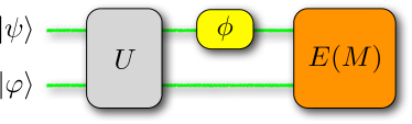
Figure 1: (Color online) The upper panel shows the general scheme of an interferometric setup. A factorized pure state $\left|{\psi}\right\rangle\left|{\varphi}\right\rangle$ of the two modes is injected in the device. The two modes are then coupled by the unitary operator $U$ and a unknown phase shift $V(\phi)$ is applied to one of the beams. At the of output the interferometer, an observable described by the POVM $E$ is measured. The lower left panel shows a schematic diagram of the passive measurement stage. Before being measured, the two beams go through a beam splitter. The difference photocurrent $D_{-}$ is then measured. In the lower right panel: scheme of the active measurement stage. The beam splitter is here replaced by an OPA. The measured observable is the sum photocurrent $D_{+}$.

In this paper we are going to consider two different classes of interferometers. In the first class we have devices employing active components, such as optical parametric amplifiers (OPAs) agar:10 . The second one, instead, includes devices with passive components, e.g. beam splitters. Active components differ from passive ones since they increase the energy of the incoming light beams, while the passive ones keep it constant. The action of an OPA on a two-mode state is described by the unitary operator

$$U_{{\rm OPA}}(\zeta)=\mathrm{exp}\{\zeta\,a^{\dagger}b^{\dagger}-\zeta^{\ast}\,a\,b\},$$

where $a$ and $b$ are the two field operators describing modes, and $\zeta\in\mathbb{C}$ is a coupling constant, linked to the gain of the amplifier. A beam splitter is instead described by the unitary

$$U_{{\rm BS}}(\nu)=\mathrm{exp}\{\nu\,a^{\dagger}b-\nu^{\ast}\,a\,b^{\dagger}\},$$

where $\nu\in\mathbb{C}$ is a coupling constant which determines the transmissivity of the beam splitter.

The performances of both classes of interferometers may be assessed using quantum estimation theory , which provides tools to find the optimal working regimes, i.e. the optimal input signals and the optimal detection stage (see Sect. IV)CS:JOSAB . However, the realization of the optimal detection stage is usually challenging with current technology and thus it becomes relevant to assess the precision achievable by feasible schemes. In this paper we consider two specific measurement schemes, characterized by their passive/active nature, optimizing their performances over the input signals in different configurations.

In the passive detection scheme, the two radiation beams interferes at a beam splitter and then are detected by two photodetectors, which count the number of photons. In this case, the measured observable is the difference photocurrent

$$D_{-}=a^{\dagger}a-b^{\dagger}b$$

between the signals, i.e. the state just before the detectors

$$|\Psi_{\scriptscriptstyle OUT}\rangle\rangle=U_{{\rm BS}}^{\dagger}(\nu)V(\phi)U\,|\Psi_{\scriptscriptstyle IN}\rangle\rangle\,.$$ (16)

In the active configuration, the beams splitter is replaced by an OPA and the measured observable is now the sum photocurrent

$$D_{+}=a^{\dagger}a+b^{\dagger}b,$$

i.e. the total number of photon of the output signals, which, in this case, are described by the state

$$|\Psi_{\scriptscriptstyle OUT}\rangle\rangle=U_{{\rm OPA}}^{\dagger}(\zeta)V(\phi)U|\Psi_{\scriptscriptstyle IN}\rangle\rangle$$ (17)

The two possible detection stages are schematically depicted in the lower panel of Fig. 1.

IV QFI for passive and active interferometers

Here we briefly review the optimal performances achievable by passive and active interferometers CS:JOSAB with Gaussian input signals. Results will serve as a referece to assess the performances of the four concrete configurations analyzed in the following Section.

IV.1 Passive quantum interferometer

The scheme of a typical passive interferometer is described in Fig. 1, where the unitary operator $U$ represents a 50:50 beam splitter, and the input states $\left|{\psi}\right\rangle\left|{\phi}\right\rangle$ are assumed to be two displaced-squeezed states. The QFI is, by definition, optimized over all the possible measurements, and therefore we do not define any measurement stage. The two input states can be written as $\left|{\alpha,\xi}\right\rangle\left|{\gamma,\zeta}\right\rangle$, where $\alpha,\gamma\in\mathbb{R}$ are the coherent coefficients (no phase is considered), and $\xi\in\mathbb{R}^{+}$, $\zeta\in\mathbb{C}$ are the squeezing coefficients, where the complex phase is accounted only for the second one. The parameter $\zeta$ can be decomposed as $\zeta=re^{-i\theta}$, where $r\in\mathbb{R}^{+}$ is its modulus, while $\theta\in[0,2\pi)$ is the phase. The QFI $H_{\phi}$ may be evaluated using Eq. (11), starting from the first-moment vector and the covariance matrix after the beam splitter, we have

$$H_{\phi}= \frac{1}{4}\,\Big{\{}4\,e^{2\xi}\,(\alpha+\gamma)^{2}+\cosh 4\xi+2\cos\theta\sinh 2r$$

$$\times\left(2\,(\alpha+\gamma)^{2}+\sinh 2\xi\right)+4\,(\alpha+\gamma)^{2}\cosh 2r$$

$$+\cosh 2(r-\xi)+\cosh 2(\xi+r)+\cosh 4r-4\Big{\}}$$ (18)

which depends on the coherent amplitudes and the squeezing parameters, while it is independent on the phase-shift itself, being the problem covariant.

As a matter of fact, there are several parameters involved in the optimization and thus it is useful to introduce a suitable re-parameterization to emphasize the quantities that are physicaly relevant. In particular, we are interested in the behavior of the QFI $H_{\phi}$ as a function of the overall intensity (i.e., the total number of photons) of the input beams. The first parameter we introduce is the coherent trade-off coefficient $\delta=\alpha^{2}/(\alpha^{2}+\gamma^{2})$, $\delta\in[0,1]$ , assessing the fraction of coherent photons in each input beams. Then, we denote by $N_{\mathrm{tot}}$ the total average number of photons of the system, accounting for both coherent and squeezed photons, as $N_{\mathrm{tot}}=\alpha^{2}+\gamma^{2}+\sinh^{2}\xi+\sinh^{2}r$. To describe the squeezing properties of the beams, we use the parameters $\beta_{\mathrm{tot}}$ and $\beta$. The first one is the fraction of (total) squeezed photons, namely $\beta_{\mathrm{tot}}=(\sinh^{2}\xi+\sinh^{2}r)/N_{\mathrm{tot}}$, $\beta_{\mathrm{tot}}\in[0,1]$. The second one is the ratio between the average number of squeezed photons in one branch and the total average number of photons, namely, $\beta=\sinh^{2}\xi/N_{\mathrm{tot}}$, $\beta\in[0,\beta_{\mathrm{tot}}]$.

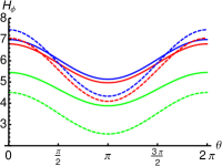
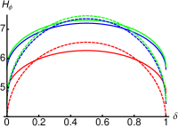
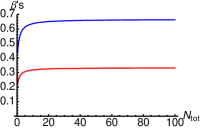
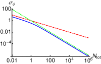
Figure 2: (Color online) (upper left) The $H_{\phi}$ as a function of $\theta$, where $N_{\mathrm{tot}}=1$, and $\delta=1/4$ (red lines), $\delta=1/2$ (blue lines), and $\delta=1$ (green lines). Solid lines for $\beta_{\mathrm{tot}}=3/4$ and $\beta=2/3$, and dashed lines for $\beta_{\mathrm{tot}}=1/3$ and $\beta=1/6$. (upper right) The $H_{\phi}$ as a function of $\delta$, where $N_{\mathrm{tot}}=1$, and $\theta=0$. Solid lines for $\beta_{\mathrm{tot}}=3/4$, dashed lines for $\beta_{\mathrm{tot}}=1/3$, and red lines for $\beta=0$, blue lines for $\beta=\beta_{\mathrm{tot}}/4$, and green lines for $\beta=\beta_{\mathrm{tot}}/2$. (lower left) The values of $\beta_{\mathrm{tot}}$ (blue line), and $\beta$ (red line) maximizing the Quantum Fisher Information $H_{\phi}$, as a function of $N_{\mathrm{tot}}$. (lower right) The standard deviation $\sigma_{\phi}$ (blue solid line), as a function of $N_{\mathrm{tot}}$. The shot-noise limit $1/\sqrt{N_{\mathrm{tot}}}$ is the red dashed line, and the Heisenberg limit $1/N_{\mathrm{tot}}$ is the green dotted line.

In Fig. 2 we illustrate the features of the QFI by showing its behavior as a function of a given parameter and by fixing the others. Looking at the upper left panel we see that $H_{\phi}$ is maximized by choosing the squeezing phase $\theta$ of equal to $0$ (or $2\pi$) independently on the value of the other parameters (while the actual value of the maximum depends on the other involved parameters). This means that optimal input signals should have the same squeezing phase, i.e. squeezing may be chosen real without loss of generality (or more generally, in phase with the coherent amplitudes). Concerning the dependence on $\delta$, the upper right panel of Fig. 2 shows that $H_{\phi}$ is maximized by $\delta=1/2$ independently on the other parameters, i.e in the optimal input signals the average number of the coherent photons in the two input states should be the same. Finally, in the lower left panel of Fig. 2, we show the optimal values of $\beta_{\mathrm{tot}}$ (blue line) and $\beta$ (red line) maximizing $H_{\phi}$. Interestingly, the optimal $\beta$ is equal to $\beta_{\mathrm{tot}}/2$ and, in the limit $N_{\mathrm{tot}}\gg 1$, $\beta_{\mathrm{tot}}\to 2/3$. Therefore, we conclude that in the optimal case the squeezing has to be balanced between the two input states, and we also need a given number of coherent photons.

Overall, the optimization reveals that the best input signals correspond to two identical displaced-squeezed states $\left|{\alpha,r}\right\rangle$. It is worth noting that the state of the system after the beam splitter is factorised, and is equal to $\left|{\sqrt{2}\alpha,r}\right\rangle\left|{0,r}\right\rangle$, where $\left|{\sqrt{2}\alpha,r}\right\rangle$ undergoes a phase shift, while $\left|{0,r}\right\rangle$ plays the role of a quantum-enhanced phase reference tra11 . The maximized QFI may be written as CS:JOSAB :

$$H_{\phi}^{\rm max}(N_{\mathrm{tot}})=\frac{4N_{\mathrm{tot}}}{9}\left[2\,\sqrt{N_{\mathrm{tot}}(N_{\mathrm{tot}}+3)}+4\,N_{\mathrm{tot}}+9\right],$$

which in the high-energy limit ($N_{\mathrm{tot}}\gg 1$) reduces to $H_{\phi}^{\rm max}(N_{\mathrm{tot}})\approx 8/3\,(N_{\mathrm{tot}}^{2}+2\,N_{\mathrm{tot}})$.

The minimum detectable fluctuation of the phase $\phi$ can now be obtained using the Cramér-Rao bound, Eq. (1). In the lower right panel of Fig. 2 we show the behaviour of $\sigma_{\phi}=1/H_{\phi}$, i.e. the minimum detectable fluctuation of $\phi$, as a function of the total energy. We have employed quantum states of light, and indeed the sensitivity is enhanced compared to the shot-noise limit, achieving the Heisenberg scaling. Moreover, having maximized the QFI in the most general case (for a passive device), we have found the actual ultimate limit for the precision of this kind of interferometer.

IV.2 Active quantum interferometer

We consider active interferometer that employs an OPA in place of the beam splitter. The scheme is shown in Fig. 1, where the unitary operator represents the action of the OPA. Since the quantumness needed to beat the shot-noise limit is now provided by the OPA, we are led to consider just coherent states as input signals. Besides, we assume that the two coherent amplitudes are real namely, $\left|{\alpha}\right\rangle\left|{\gamma}\right\rangle$, with $\alpha,\gamma\in\mathbb{R}$, i.e. the two signals have the same phase. As we will see in the following, this choice lead to Heisenberg scaling of sensitivity. The unitary operator describing the amplifier is $U_{\rm OPA}(\zeta)$, where $\zeta=r\,e^{-i\theta}$ is the squeezing coefficient, $r\in\mathbb{R}^{+}$ and $\theta\in[0,2\pi)$. Upon using again Eq. (11), starting from the first-moment vector and the covariance matrix after the OPA, we have

$$H_{\phi}= \alpha^{2}+\gamma^{2}+\left(\alpha^{2}+\gamma^{2}+\frac{1}{2}\right)\cosh 4r$$

$$+2\,\alpha\gamma\cos\theta\sinh 4r+2\,(\alpha^{2}-\gamma^{2})\cosh 2r-\frac{1}{2}$$ (19)

As in the case of passive interferometers, we want to write the QFI as a function of suitable parameters, related to the energetic properties of the light beams. To this aim, we still use the coherent trade-off coefficient $\delta\in[0,1]$, introduced above, and the total average number of photons (including those introduced with the OPA) $N_{\mathrm{tot}}=(\alpha^{2}+\gamma^{2}+1)\cosh 2r+4\,\alpha\gamma\cos\theta\sinh r\cosh r-1$, $N_{\mathrm{tot}}\in[0,\infty]$. The last parameter we define is the ratio between the number of squeezed photons and the total number of photons, namely, $\beta=2\,\sinh^{2}r/N_{\mathrm{tot}}$, $\beta\in[0,1]$.

In order to maximize the QFI $H_{\phi}$, we analyze its behavior as a function of $\theta$ and $\delta$ for fixed $\beta$ and $N_{\mathrm{tot}}$. The typical behaviour is shown in the upper left panel of Fig. 3. As a matter of fact, the maximum is achieved for $\theta=\pi$ independently on the other parameters, while the optimal value of $\delta$ depends on $\beta$ and $N_{\mathrm{tot}}$ (we found that $\delta>1/2$). Given $N_{\mathrm{tot}}$, in order to find the values of $\beta$ and $\delta$ maximizing the QFI we should use a numerical maximization. The results are shown in the upper right panel of Fig. 3, where the minimum detectable fluctuation of the phase $\phi$ is plotted. Remarkably, also with an active interferometer the Heisenberg limit can be achieved agar:10 ; CS:JOSAB . In the lower panel of Fig. 3, we show the values of $\delta_{\mathrm{max}}$ and $\beta_{\mathrm{max}}$ maximising $H_{\phi}$ as functions of $N_{\mathrm{tot}}$. In the high-energy case ($N_{\mathrm{tot}}\gg 1$) the parameter $\delta_{\mathrm{max}}$ is equal to $1/2$, while $\beta_{\mathrm{max}}$ is equal to $2/3$ leading to the following analytic expression for the QFI:

$$H^{\rm max}(N_{\mathrm{tot}})\approx\frac{4}{3}\,\left(N_{\mathrm{tot}}^{2}+2N_{\mathrm{tot}}\right)\qquad(N_{\rm tot}\gg 1).$$

It is worth noting that in order to achieve this value, two coherent states with the same number of photons have to be injected in the interferometer ($\delta_{\mathrm{max}}\simeq\frac{1}{2}$ for large $N_{\mathrm{tot}}\gg 1$), and the OPA has to introduce two third of the total number of photons in the system. Therefore, in the regime $N_{\mathrm{tot}}\gg 1$ the ultimate limit of the QFI for active interferometers is proportional to the square of the total number of photons in the system.

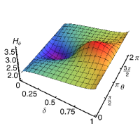
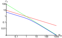
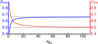
Figure 3: (Color Online) (Upper left) The QFI $H_{\phi}$ for an active interferometer as a function of $\theta$ and $\delta$, for fixed values of $\beta=0.7$ and $N_{\mathrm{tot}}=1$. (Upper right) The minimum detectable fluctuation $\sigma_{\phi}$ (blue solid line) as a function of $N_{\mathrm{tot}}$, with the shot-noise limit (red dashed line) and the Heisenberg limit (green dotted line). (Lower panel) The parameters $\beta_{\mathrm{max}}$ and $\delta_{\mathrm{max}}$, maximising $H_{\phi}$, as a function of $N_{\mathrm{tot}}$.

Summarizing, the precision achievable by active interferometers shows the same scaling of passive ones. However, passive devices offers a factor two enhacement over active ones and should thus be preferred, assuming that their implementations involve similar technological efforts. We notice that both schemes allows one to beat the classical precision limit, upon the introducti of squeezed light in the system.

V Sensitivity for passive and active interferometers

In the previous Section we evaluated the ultimate limits to precision for any phase-shift estimation scheme based on passive and active interferometers. The Cramer-Rao theorem ensures that the obtained bounds are achievable, i.e. there exists an observable which may be employed to estimate the phase-shift with optimal precision. This optimal observable, however, correspond to the spectral measure of the SLD hel76 ; par09 and it is not clear whether, and in which regimes, it may be implemented with current optical technology.

In order to assess the performances of feasible interferometers in this section we consider a realistic detection stage and analyze the sensitivity of different configurations, also taking into account possible imperfections of the detectors, such as losses leading to non unit quantum efficiency. In particular, we evaluate phase sensitivity using Eq. (14), with the observable $X$ replaced by either the difference photocurrent $D_{-}(\eta)$ in the passive measurement scheme, or by the sum photocurrent $D_{+}(\eta)$ in the active case, see Appendix A for the expression of the mean values and the variances. We optimize the input signals in all the four possible configurations (active/passive interferometers with active/passive detection stage) and compare performances in the ideal case, as well as for non unit quantum efficiency.

V.1 The passive/passive case

We now consider the passive interferometer introduced in Sec. IV.1, equipped with the passive measurement scheme described in the lower left panel of Fig. 1. This kind of device is the well-known Mach-Zehnder interferometer, also equivalent to the Michelson one employed in gravitational interferometers pez08 ; grav:11 ; raf14 ; lan13 ; lan14 . It possible to show oli:par:OptSp that in this case the best choice for the input states is $\left|{\alpha,\xi}\right\rangle\left|{0,\zeta}\right\rangle$, where $\alpha,\xi\in\mathbb{R}$ are, respectively, the coherent and squeezed coefficients of the first state and $\zeta=r\,e^{-i\theta}$ is the squeezing coefficient of the second state, $r\in\mathbb{R}^{+}$ and $\theta\in[0,2\,\pi)$. Furthermore, both the beam splitters used in the interferometer are balanced, and their phases differ by $\pi$, so that the output is equal to the input if there is no additional phase shift.

V.1.1 Ideal photodetection

We first address the ideal case, i.e. when the quantum efficiency $\eta$ is equal to one (we assume that the two detectors are equal and have the same quantum efficiency). Upon employing the parameterization introduced in Sect. IV.1 for the input signals and using Eq. (14), the sensitivity $S_{1}$ for the difference photocurrent may be evaluated analytically. We do not report its full expression since it is cumbersome and proceed with the numerical minimization. As a first step we minimize $S_{1}$ over the phase shift $\phi$ and the squeezing phase $\theta$: the typical behavior of $S_{1}$ as a function of these parameters is shown in the upper panels of Fig. 4 for different possible input configurations. As it is apparent from the plots $S_{1}$ is minimized by $\phi=\pi/2$ and $\theta=0$ independently on the other parameters. We confirmed this by scanning the full parameter range.

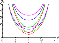
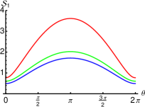
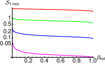
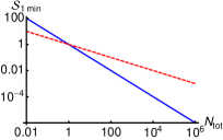
Figure 4: (Color Online) The passive/passive interferometer with ideal phodetection. In the upper left panel we show the sensitivity $S_{1}$ as a function of $\phi$, for $N_{\mathrm{tot}}=2$, $\xi=0.5$ and $r=0.7$ (solid line), or $\xi=0.7$ and $r=0.5$ (dashed line), and for $\theta=0$ (red lines), or $\pi/4$ (green), or $\pi/2$ (blue), or $3/4\,\pi$ (magenta). The upper right panel shows the sensitivity $S_{1}$ as a function of $\theta$, for $\phi=\pi/2$, $N_{\mathrm{tot}}=2$, and for $\xi=0.5$ and $r=0.7$ (red line), or $\xi=0.7$ and $r=0.5$ (blue), or $\xi=0.5$ and $r=0.5$ (green). The lower left panel shows the ideal sensitivity $S_{1\,\mathrm{min}}$, minimized with respect to $\beta$, as a function of $\beta_{\mathrm{tot}}$, for $N_{\mathrm{tot}}=10^{-1}$ (red line), or $N_{\mathrm{tot}}=1$ (green), or $N_{\mathrm{tot}}=10$ (blue), or $N_{\mathrm{tot}}=10^{2}$ (magenta). The lower right panel shows the optimized sensitivity $S_{1\,\mathrm{min}}$ as a function of $N_{\mathrm{tot}}$ (solid blue line). Also the shot-noise limit $1/\sqrt{N_{\rm tot}}$ (dashed red line) is shown.

Using this results we may write a simpler expression for $S_{1}$ in terms of the remaining parameters, which reads as follows

$$S_{1}= \,\bigg{\{}4\,(1-\beta)\beta\,N_{\mathrm{tot}}^{2}+4\,\sqrt{\beta N_{\mathrm{tot}}}\sqrt{\beta N_{\mathrm{tot}}+1}$$

$$\times\left((\beta_{\mathrm{tot}}-1)N_{\mathrm{tot}}-\sqrt{N_{\mathrm{tot}}(\beta_{\mathrm{tot}}-\beta)}\sqrt{N_{\mathrm{tot}}(\beta_{\mathrm{tot}}-\beta)+1}\right)$$

$$+2\,N_{\mathrm{tot}}\bigg{\}}^{\frac{1}{2}}/\left(\sqrt{2}\,\left|N_{\mathrm{tot}}-2\,N_{\mathrm{tot}}\beta\right|\right)$$ (20)

Results of the minimization of $S_{1}$ with respect to the squeezing fractions $\beta_{\mathrm{tot}}\in[0,1]$ and $\beta\in[0,\beta_{\mathrm{tot}}]$ are shown in the lower panels of Fig. 4. On the left we show $S_{1}$, numerically minimized with respect to $\beta$, as function of $\beta_{\mathrm{tot}}$. We find that $S_{1}$ achieves its minimum for $\beta_{\mathrm{tot}}=1$, that is, when all the energy is provided by the squeezing or, equivalently, no coherent (classical) radiation is needed. Thus, if we fix $\beta_{\mathrm{tot}}=1$, we can analytically evaluate the optimal value of $\beta$, which turns out to be $1/2$. Therefore, the optimal input system is described by two squeezed-vacuum states, which have the same phase and number of photons. Overall, the sensitivity $S_{1\,\mathrm{min}}=N_{\mathrm{tot}}^{-1}$, saturates the Heisenberg limit as a function of the total energy $N_{\mathrm{tot}}^{-1}$, see the lower right panel of Fig. 4.

V.1.2 Non unit quantum efficiency

In the realistic situation the detection efficiency is lower than one: the sensitivity $S_{\eta}(N_{\mathrm{tot}},\phi,\beta_{\mathrm{tot}},\beta,\theta)$ depends now on all the previous parameters and also on the quantum efficiency $\eta$ of the detectors (we assume the same for both). In order to minimize $S_{\eta}$ we proceed as in the ideal case. The behaviour of $S_{\eta}$ as a function of the phase shift $\phi$ and the squeezing phase $\theta$ is shown in the upper panels Fig. 5. As we found in the ideal case, the sensitivity is minimized for $\phi=\pi/2$ and $\theta=0$.

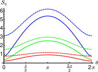
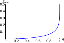
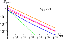
Figure 5: (Color Online) The passive/passive interferometer with realistic phodetection. In the upper left panel we show the sensitivity $S_{\eta}$ as a function of $\phi$, for $N_{\mathrm{tot}}=1$, $\beta_{\mathrm{tot}}=0.8$, and $\beta=0.6$. Solid lines for $\eta=0.9$, and $\theta=\pi/4$ (red) or $\theta=3/4\,\pi$ (blue). The dashed lines for $\eta=0.3$, with $\theta=\pi/2$ (green) or $\theta=\pi$ (magenta). The dotted lines for $\eta=0.1$, and $\theta=\pi/4$ (red) or $\theta=3/4\,\pi$ (blue). In the upper right panel: the sensitivity $S_{\eta}$ as a function of $\theta$, for $\phi=\pi/2$, $N_{\mathrm{tot}}=10$, and $\beta_{\mathrm{tot}}=0.9$. Solid lines for $\eta=0.8$, dashed lines $\eta=0.2$, and for $\beta=0.1$ (red), or $\beta=0.3$ (green), or $\beta=0.6$ (blue). In the lower right panel we show the fraction $\beta_{\mathrm{min}}$, minimizing the sensitivity $S_{\eta}$ for $N_{\rm tot}\ll 1$, as a function of $\eta$. In the lower right panel: the optimized sensitivity for $N_{\rm tot}\gg 1$ as a function of $N_{\mathrm{tot}}$, for $\eta=0.9$ (blue), or $\eta=0.4$ (magenta), $\eta=0.1$ (orange). The shot-noise (red dashed line) and the Heisenberg limit (green dotted line) are also shown.

In order to solve the optimization problem, we now consider the sensitivity $S_{\eta}$ in the low-energy regime ($N_{\mathrm{tot}}\ll 1$) and in the high-energy regime ($N_{\mathrm{tot}}\gg 1$). When $N_{\mathrm{tot}}\ll 1$, the sensitivity can be expanded to the leading term as follow

$$S_{\eta\,\mathrm{min}}(N_{\mathrm{tot}},\beta_{\mathrm{tot}},\beta)\approx\sqrt{\frac{1-2\eta\sqrt{\beta(\beta_{\mathrm{tot}}-\beta)}}{\eta(1-2\beta)^{2}}}\,\frac{1}{\sqrt{N_{\mathrm{tot}}}}.$$ (21)

The coefficient multiplying $1/\sqrt{N_{\mathrm{tot}}}$ is minimised when $\beta_{\mathrm{tot}}=1$, and $\beta$ depends on $\eta$ as shown in the lower left panel of Fig. 5. For $\eta<1$, we find that the optimal working regime is obtained when we introduce more squeezed photons in one arm than in the other. The optimized sensitivity is then given by

$$S_{\eta\,\mathrm{min}}(N_{\mathrm{tot}})=\sqrt{\frac{1}{2\eta}+\frac{1}{2}\,\sqrt{\frac{1-\eta^{2}}{\eta^{2}}}}\,\frac{1}{\sqrt{N_{\mathrm{tot}}}}.$$ (22)

Let us now focus to the high-energy regime ($N_{\mathrm{tot}}\gg 1$), in which the sensitivity can be expanded as

$$S_{\eta\,\mathrm{min}}(N_{\mathrm{tot}},\beta)\approx\sqrt{\frac{1-\eta}{\eta(1-2\beta)^{2}}}\,\frac{1}{\sqrt{N_{\mathrm{tot}}}},$$ (23)

where the coefficient $\beta_{\mathrm{tot}}$ does not explicitly appear, but affects the coefficients of higher orders. However, we can safety set $\beta_{\mathrm{tot}}\neq 1$ and consider only the first order. In order to minimise the sensitivity of Eq. (23), we can set $\beta=0$ (or $\beta=1$), that is, all the squeezing photons can be injected in one arm. Thus, the optimal sensitivity turns out to be

$$S_{\eta\,\mathrm{min}}(N_{\mathrm{tot}})=\sqrt{\frac{1-\eta}{\eta}}\,\frac{1}{\sqrt{N_{\mathrm{tot}}}}$$ (24)

and we show its behaviour, for different values of $\eta$, in the lower right panel of Fig. 5.

It is worth noting that the sensitivity in presence of noise scales as the shot noise limit, that is $1/\sqrt{N_{\mathrm{tot}}}$. Therefore, using quantum (squeezed) radiation inside an interferometer allows to improve the sole coefficient multiplying the shot-noise limit oli:par:OptSp .

V.2 The passive/active case

This interferometer is composed by a beam splitter, mixing the light beams before the phase shift, and by an active measurement scheme where an amplifier is used to recombine the modes, adding squeezing before the photodetection. The input states for this interferometers are $\left|{\alpha,\xi}\right\rangle\left|{\gamma}\right\rangle$, where $\alpha,\gamma\in\mathbb{R}$ are the coherent amplitudes and $\xi=r\,e^{-i\theta}$ is the squeezing coefficient of the first state, $r\in\mathbb{R}^{+}$ and $\theta\in[0,2\,\pi)$. Furthermore, the beam splitters is balanced and its phase is set equal to zero, while the OPA is parametrised by a squeezing coefficient $\zeta=r_{1}\,e^{-i\theta_{1}}\in\mathbb{C}$, where $r_{1}\in\mathbb{R}^{+}$, and $\theta_{1}\in[0,2\pi)$.

V.2.1 Ideal photodetection

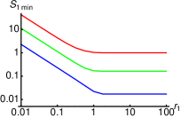
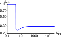
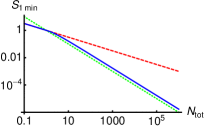
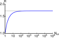
Figure 6: (Color online) The passive/active interferometer with ideal photodetection. The upper left panel shows the minimized sensitivity $S_{1\,\mathrm{min}}$ as a function of the parameter $r_{1}$, for $N_{\mathrm{tot}}=1$ (red line), $N_{\mathrm{tot}}=10$ (green line), and $N_{\mathrm{tot}}=100$ (blue line). The upper right panel shows the parameter $\beta$ minimizing the sensitivity as a function of $N_{\mathrm{tot}}$. The lower left panel shows the optimal sensitivity $S_{1\,\mathrm{min}}$ as a function of the total number of photons $N_{\mathrm{tot}}$, together with the shot-noise limit (red dashed line) and the Heisenberg limit (green dotted line). The lower right panel illustrate the behaviour of the ratio $R=S_{1\,\mathrm{min}}/S_{\mathrm{HL}}$, where $S_{\mathrm{HL}}=1/N_{\mathrm{tot}}$ is the Heisenberg scaling, as a function of $N_{\mathrm{tot}}$. The asymptotic value of $R$ is $1+1/\sqrt{2}$.

The ideal $S_{1}$ depends on the coherent amplitudes $\alpha$ and $\gamma$ and on the squeezing ones $\xi=re^{-i\theta}$, and $\zeta=r_{1}e^{-i\theta_{1}}$. In the following we will use the same parameterization introduced in sect. IV.1. The ideal sensitivity is a cumbersome function $S_{1}(N_{\mathrm{tot}},\delta,\phi,\beta,\theta,r_{1},\theta_{1})$, which we do not report here. However, from its analytic expression, one may observe that the phase of the OPA, $\theta_{1}$, can be set equal to zero without loss of generality. We now focus on the behavior of the sensitivity when the amplifier introduces squeezed photons in the system. As we have done in the previous cases, we have numerically minimized $S_{1}$ with respect to all the parameters except $N_{\rm tot}$ and $r_{1}$. The behaviour of sensitivity is shown in the upper left panel of Fig. 6: in the limit $r_{1}\gg 1$, the sensitivity reaches its minimum. Therefore, the optimal sensitivity is obtained when a large number of squeezed photons is introduced by the amplifier.

From the analysis of the numerical minimization, we find that the optimal value of the coherent trade-off coefficient $\delta$ is 1. In this case, the best configuration for the estimation of the phase is obtained when the input system is described by the state $|\Psi_{\scriptscriptstyle IN}\rangle\rangle=\left|{\alpha,\xi}\right\rangle\left|{0}\right\rangle$. Concerning the squeezing fraction $\beta$, we found that the optimal value $\beta_{\hbox{min}}$ minimising $S_{1}$ depends in a non-trivial way on the number of photons of the input state, as shown in the upper right panel of Fig. 6. Remarkably, in the limit of high energy the parameter is $\beta_{\mathrm{min}}\approx 0.3$. Thus, the optimal estimation of $\phi$ is obtained when both coherent and squeezed photons are used. In the low-energy range, the value of $\beta_{\mathrm{min}}$ is equal to 1, and thus the optimal state of the system is $\left|{0,\xi}\right\rangle\left|{0}\right\rangle$: only squeezed light is needed.

The optimized sensitivity $S_{1\,\mathrm{min}}$ is shown in the the lower left panel of Fig. 6. In the high-energy regime, the sensitivity is proportional to the Heisenberg limit, even if with coefficient larger than one. In the low-energy range, the sensitivity goes down to the shot-noise limit. In order to assess the sensitivity when $N_{\mathrm{tot}}\gg 1$, we consider the ratio $R=S_{1\,\mathrm{min}}/S_{\mathrm{HL}}$ between the numerically minimized $S_{1\,\mathrm{min}}$ and the Heisenberg scaling (Fig. 6, lower right panel): we find that, in the high-energy regime

$$R\stackrel{{\scriptstyle N_{\mathrm{tot}}\gg 1}}{{\longrightarrow}}\left(1+\frac{1}{\sqrt{2}}\right)\,.$$ (25)

V.2.2 Non unit quantum efficiency

For non unit quantum efficiency the sensitivity is expressed as a function $S_{\eta}(N_{\mathrm{tot}},\delta,\phi,\beta,\theta,r_{1},\theta_{1})$. We analyze its behaviour starting from its dependence on the parameter $r_{1}$, which corresponds to the energy (average number of squeezed photons) introduced by the parametric amplifier. In the ideal case, we have seen that the optimal sensitivity is obtained for $r_{1}\gg 1$. To analyze the behavior of $S_{1}$ in the presence of detection loss, we minimize it with respect to all the parameters, except for $N_{\mathrm{tot}}$, $\eta$, and $r_{1}$. The optimal value $S_{\eta}(N_{\mathrm{tot}},r_{1})$ is shown in Fig. 7, for different values of the total number of photons $N_{\mathrm{tot}}$ and quantum efficiency $\eta$. From the plot we can extract two main results. First of all, also for non unit quantum efficiency, the sensitivity is optimized for $r_{1}\gg 1$. Therefore, in the optimal configuration, we have to provide as many photons as possible through the amplifier. Moreover, if a large amount of energy is introduced inside the system with the amplifier, sensitivity approaches the ideal one, as it may be seen by taking the limit of $S_{\eta}$ for $r_{1}\rightarrow\infty$. Therefore, the active measurement stage allows us to balance the losses of the detectors, and to obtain the ideal sensitivity even in the presence of noise. Since the real sensitivity is minimized for $r_{1}\gg 1$, and we have shown that in that regime the real and ideal sensitivities coincide, we can use the same results from the ideal case. Thus, we find that the sensitivity is still proportional to the Heisenberg limit, even if the system is affected by noise.

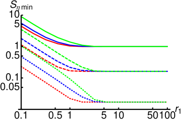
Figure 7: (Color online) The passive/active interferometer with realistic photodetection. The plot shows the optmized sensitivity $S_{\eta\,\mathrm{min}}$ as a function of $r_{1}$, for $N_{\mathrm{tot}}=1$ (solid line), $N_{\mathrm{tot}}=10$ (dashed line), and $N_{\mathrm{tot}}=100$ (dotted line), and for $\eta=1$ (red line), $\eta=0.6$ (blue line), and $\eta=0.2$ (green line).

V.3 The active/passive case

Now we turn our attention to the performances of the active interferometer of Sec. IV.2, when a passive measurement stage is employed. The input beams are described by two coherent states, $\left|{\alpha}\right\rangle$ and $\left|{\gamma}\right\rangle$, respectively, where we take $\alpha,\gamma\in{\mathbbm{R}}$. The first component of the interferometer is the OPA, described by the operator $U_{{\rm OPA}}(\xi)$, with $\xi=re^{-i\theta}$, where $r\in\mathbb{R}^{+}$, and $\theta\in[0,2\pi)$. Finally, the beam splitter inside the measurement stage is assumed to be balanced.

V.3.1 Ideal photodetection

In order to analyze the sensitivity $S_{1}$ in the ideal scenario, i.e. $\eta=1$, we consider the following parameters: First, the total number of photons, here given by $N_{\mathrm{tot}}=\left(\alpha^{2}+\gamma^{2}+1\right)\cosh 2r+4\,\alpha\gamma\cos\theta\sinh r\cosh r-1$, which accounts for both the photons in the input signals as well as those introduced by the amplifier. Then, we consider the ratio $\delta$ between the number of coherent photons in the two input states, as defined in Sec. IV.1, and the squeezing fraction $\beta=2\,\sinh^{2}r/N_{\mathrm{tot}}$, expressing the ratio between the number of squeezed photon injected by the amplifier and the total number of photons. In the following, we thus consider $S_{1}=S_{1}(N_{\mathrm{tot}},\delta,\phi,\beta,\theta)$.

As in the previous sections, we want to minimize $S_{1}$ to obtain a function of the sole average number of photons $N_{\mathrm{tot}}$. To this aim, we numerically minimize $S_{1}$ and find that the coherent trade-off coefficient $\delta$ should be $\delta=1/2$ (the procedure is similar to previous cases, we do not report the details), i.e. the number of coherent photons in the input signals should be balanced. Similarly, one finds that the optimal value $\phi=\pi/2$ is independent on the other parameters.

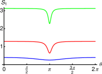
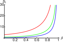
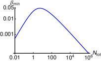
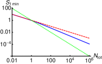
Figure 8: (Color online) The active/passive interferometer with ideal photodetection. In the upper left panel we show the sensitivity $S_{1}$ as a function of $\theta$, when $N_{\mathrm{tot}}=10$, $\delta=1/2$ and $\phi=\pi/2$. The blue line refers to $\beta=0.01$, the red line to $\beta=1/3$, and the green one to $\beta=2/3$. The upper right panel shows the sensitivity $S_{1}$ as a function of $\beta$, when $\delta=1/2$, $\phi=\pi/2$, and $\theta=\pi$. The red line is taken for $N_{\mathrm{tot}}=0.1$, the green one for $N_{\mathrm{tot}}=1$, and the blue one for $N_{\mathrm{tot}}=10$. The lower left panel shows the value of $\beta$ minimizing $S_{1\,\mathrm{min}}$, as a function of $N_{\mathrm{tot}}$. Finally, the lower right panel shows the optimized $S_{1}$ as a function of $N_{\mathrm{tot}}$ (blue line), with the shot-noise limit (red dashed line) and the Heisenberg limit (green dotted line).

We now consider the parameter $\theta$, that is the phase introduced by the amplifier. The value of $S_{1}$ as a function of $\theta$ is shown in the upper left panel of Fig. 8, for different values of the parameter $\beta$. The plot shows that the value of $\theta$ minimizing the sensitivity is $\pi$. It is worth noting, moreover, that $S_{1}$ grows with $\beta$. Therefore, it seems that the best estimation possible is achieved for small values of $\beta$. In the upper right panel of Fig. 8, we show the sensitivity as a function of the parameter $\beta$, showing that $S_{1}$ is indeed minimized for values of $\beta$ close to zero. However, a small fraction of squeezing is necessary, otherwise the sensitivity would be equal to the shot-noise limit $1/\sqrt{N_{\mathrm{tot}}}$. In the lower left panel of the same figure the value $\beta_{\mathrm{min}}$ minimizing $S_{1}$ is shown as a function of $N_{\mathrm{tot}}$. It grows with $N_{\mathrm{tot}}$ until it reaches a maximum for $N_{\mathrm{tot}}\approx 10$, close to the value $\beta_{\mathrm{min}}\simeq 0.05$, and then it decreases as the total number of photons increase.

After the minimization of $S_{1}$, it is interesting to analyze how it behaves as the total number $N_{\rm tot}$ of photons is changed. This is illustrated in the lower right panel of Fig. 8. In the low-energy regime ($N_{\mathrm{tot}}\ll 1$), the optimal sensitivity is equal to the shot noise limit, whereas in the high-energy regime, $N_{\mathrm{tot}}\gg 1$), we have that $S_{1\,\mathrm{min}}$ is below the the shot-noise limit, but above the Heisenberg limit. Actually, $S_{1\,\mathrm{min}}$ is proportional to $N_{\mathrm{tot}}^{-2/3}$ in the high-energy regime.

V.3.2 Non unit quantum efficiency

In a realistic situation, when $\eta<1$, the sensitivity is a function $S_{\eta}(N_{\mathrm{tot}},\delta,\beta,\phi,\theta)$. An analytic, though cumbersome, expression for $S_{\eta}$ may obtained: we are not reporting it here. We start by noting that, as it happens for the other configurations, the sensitivity $S_{\eta}$ is still minimized by $\delta=1/2$, $\phi=\pi/2$, i.e. also for the active/passive case a non unit quantum quantum efficiency does not influence the position of the minimum of the sensitivity, at least for what concerns the phases of the system.

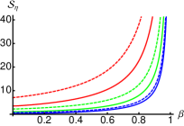
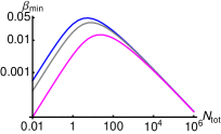
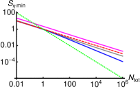
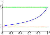
Figure 9: (Color online) The active/passive inteferometer with realistic photodetection. The upper left panel shows the sensitivity $S_{\eta}$ as a function of $\beta$, for $\delta=1/2$, $\phi=\pi/2$, and $\theta=\pi$. The solid lines are for $\eta=0.8$, and the dashed lines for $\eta=0.2$. The red lines are for $N_{\mathrm{tot}}=0.1$, green lines for $N_{\mathrm{tot}}=1$, and blue lines for $N_{\mathrm{tot}}=10$. In the upper right panel the value of $\beta$ minimizing $S_{\eta}$ is shown as a function of $N_{\mathrm{tot}}$. The blue line refers to $\eta=1$, the grey one to $\eta=0.6$, and magenta one to $\eta=0.2$. The lower left panel shows the optimized sensitivity $S_{\eta\,\mathrm{min}}$ as a function of $N_{\mathrm{tot}}$, for $\eta=1$ (blue line), $\eta=0.8$ (grey line) and $\eta=0.2$ (magenta line). The shot-noise limit (red dashed line) and the Heisenberg limit (green dotted line) are shown. The lower right panel shows the exponent $\epsilon(\eta)$ as a function of the quantum efficiency.

Using this result we may write the sensitivity as

$$S_{\eta}= \,\Bigg{\{}\Big{[}\eta(\beta-2)\beta^{2}N_{\mathrm{tot}}^{2}-\eta\beta+\beta N_{\mathrm{tot}}(\eta(\beta-3)-1)$$

$$+\sqrt{\beta N_{\mathrm{tot}}(\beta N_{\mathrm{tot}}+2)}(\eta(1-(\beta-2)\beta N_{\mathrm{tot}})+1)-1\Big{]}$$

$$/\Big{[}\eta(\beta-1)^{2}N_{\mathrm{tot}}\left(\sqrt{\beta N_{\mathrm{tot}}(\beta N_{\mathrm{tot}}+2)}-1-\beta N_{\mathrm{tot}}\right)\Big{]}\Bigg{\}}^{\frac{1}{2}}\,,$$ (26)

which now depends on the total number of photons, on the squeezing fraction and on the quantum efficiency $\eta$. We minimize the sensitivity with respect to the squeezing fraction $\beta$. In Fig. 9 (upper left panel), the sensitivity is shown as a function of $\beta$. The best sensitivity is achieved, again, for values of $\beta$ close to $0$. The actual value of $\beta$ minimizing the sensitivity is shown in the upper right panel of Fig. 9 for different values of $\eta$. The overall behavior is similar to the ideal case, even if we need less and less squeezing as the quantum efficiency decreases.

The optimum sensitivity is thus obtained when two identical coherent states are injected in the interferometer, and when the amplifier introduces only a small fraction of squeezed photons. In the lower left panel of Fig. 9, the optimized sensitivity, as a function of the total number of photons is plotted for different values of $\eta$. Notice that, in the high-energy regime, the sensitivity gradually approaches the shot-noise limit as the quantum efficiency decreases. In the limit $N_{\rm tot}\gg 1$ the sensitivity depends on the total number as a power-law $N_{\rm tot}^{-\epsilon(\eta)}$, where the function $\epsilon(\eta)$ is shown in the lower right panel of Fig. 9. The coefficient $\epsilon$ decreases from the value $2/3$ to $1/2$ (the shot-noise limit) as the quantum efficiency decreases. Compared to the Mach-Zehnder interferometer studied in sect. V.1, the active interferometer we have analyzed here has a sensitivity which approaches the shot-noise limit only for $\eta\rightarrow 0$. Thus, despite this interferometer does not allow us to reach the Heisenberg limit, its sensitivity improves over that of a Mach-Zender interferometer, at least for $\eta$ not to far from unit.

V.4 The active/active case

We now study the sensitivity of the active interferometer of Sect. IV.2, with an active measurement stage. The sensitivity of this interferometer was studied in Ref. agar:10 , though only in the ideal case.

The input signals here are two coherent states, $\left|{\alpha}\right\rangle$ in the first mode, and $\left|{\gamma}\right\rangle$ in the second one. We can take, without loss of generality, both $\alpha$ and $\gamma$ real. The interferometer involves two amplifiers, described by the same unitary operator $U(\xi_{j})$, with $j=1,2$. The coefficient $\xi_{1}$ is complex, while $\xi_{2}$ can takes real values without loss of generality. We rewrite $\xi_{1}=r_{1}e^{-i\theta_{1}}$, and $\xi_{2}=r_{2}$, where $r_{1},r_{2}\in\mathbb{R}^{+}$, and $\theta_{1}\in[0,2\pi)$.

V.4.1 Ideal photodetection

Te sensitivity is a function $S_{1}(\alpha,\gamma,\phi,r_{1},\theta_{1},r_{2})$. As we have done for other configurations, we introduce a convenient parametrization to better capture the energy lanscape of the system. The first parameter is the total number of photons, $N_{\mathrm{tot}}$, resulting from the input signals and the first amplifier. This parameter can be expressed as $N_{\mathrm{tot}}=\left(\alpha^{2}+\gamma^{2}+1\right)\cosh 2r_{1}+4\,\alpha\gamma\cos\theta\sinh r_{1}\cosh r_{1}-1$. The second parameter is the coherent trade-off coefficient $\delta$, introduced in sect. IV.1. The last parameter we consider is the squeezing fraction of photons introduced by the first amplifier, namely, $\beta=2\,\sinh^{2}r_{1}/N_{\mathrm{tot}}$, taking values between $0$ and $1$. The ideal sensitivity turns out to be a function $S_{1}(N_{\mathrm{tot}},\delta,\phi,\beta,\theta_{1},r_{2})$.

In Sect. V.2, we have seen that the sensitivity of a passive interferometer is minimised when the amplifier in the active measurement stage injects a large number of photons. We study the sensitivity of the active interferometer in the same limit, since the state arriving at the detection stage lies in the same Gaussian sector. In order to validate this choice, the sensitivity $S_{1}$ is numerically minimised with respect to all the parameters, except for $N_{\mathrm{tot}}$ and $r_{2}$. Results are shown in the upper left panel of Fig. 10, confirming that the sensitivity is minimized when the OPA introduces a large number of photons before the measurement. Thus, we study the sensitivity in the limit of $r_{2}\rightarrow\infty$.

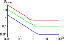
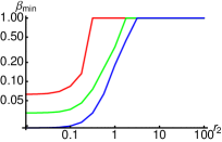
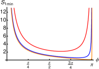
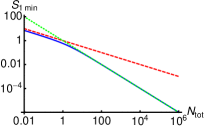
Figure 10: (Color Online) The active/active interferometer with ideal photodetection. The upper left panel shows the minimum ideal sensitivity $S_{1\,\mathrm{min}}$ as a function of $r_{2}$, for $N_{\mathrm{tot}}$ equal to $1$ (red line), $10$ (green line), and $100$ (blue line). In the upper right panel we show the value of $\beta$ minimizing $S_{1}$ as a function of $r_{2}$, for the same values of $N_{\mathrm{tot}}$ of the left plot. In the lower left panel we show the sensitivity $S_{1\,\mathrm{min}}$ as a function of $\phi$, for $N_{\mathrm{tot}}$ equal to $0.1$ (red line), $1$ (blue line), and $10$ (orange one). The lower right panel shows the sensitivity $S_{1\,\mathrm{min}}$ as a function of $N_{\mathrm{tot}}$. The shot noise (red dashed) and the Heisenberg limit (green dotted) are also shown for comparison.

It is interesting to notice that, when $r_{2}\gg 1$, the sensitivity $S_{1}$ is minimised for $\beta=1$. This is shown in the upper right panel of Fig. 10 where the value of $\beta$ minimizing the sensitivity is shown as a function of $r_{2}$ for different values of $N_{\mathrm{tot}}$. In other words, as far as $r_{2}\gg 1$, the optimal sensitivity is obtained when all the photons are introduced inside the interferometer with the first amplifier. No coherent radiation is needed and the input signal is just the vacuum in both modes. Since the input state is vacuum, the coherent trade-off coefficient $\delta$ loses its meaning, and in fact we find that the sensitivity does not longer depend on it. Moreover, it is possible to show that the analytic expression of $S_{1}$, after setting $\beta=1$ is given by

$$S_{1\,\mathrm{min}}= \Bigg{\{}\Big{[}\csc^{2}(\theta_{1}-\phi)\Big{(}N_{\mathrm{tot}}(N_{\mathrm{tot}}+2)\cos 2(\theta_{1}-\phi)$$

$$+4\,(N_{\mathrm{tot}}+1)\sqrt{N_{\mathrm{tot}}(N_{\mathrm{tot}}+2)}\cos(\theta_{1}-\phi)$$

$$+3\,N_{\mathrm{tot}}(N_{\mathrm{tot}}+2)+2\Big{)}\Big{]}/\Big{[}2\,N_{\mathrm{tot}}(N_{\mathrm{tot}}+2)\Big{]}\Bigg{\}}^{\frac{1}{2}}\,.$$ (27)

The sensitivity depends only on the difference between $\theta_{1}$ and $\phi$ and we can thus neglect one of them, e.g. $\theta_{1}$. The last parameter to consider in order to optimize the sensitivity is the phase $\phi$. In the lower left panel of Fig. 10, we show $S_{1}$ as a function of $\phi$. It is possible to see that the minimum is achieved for values of $\phi$ close to $\pi$, though the exact value changes with $N_{\mathrm{tot}}$. Eventually, the analytic form of the optimal sensitivity is given by

$$S_{1\,\mathrm{min}}(N_{\mathrm{tot}})=\frac{1}{\sqrt{N_{\mathrm{tot}}(N_{\mathrm{tot}}+2)}}$$ (28)

which approaches the Heisenberg limit $N_{\rm tot}^{-1}$ in the high-energy regime $N_{\mathrm{tot}}\gg 1$. The behaviour of the sensitivity as a function of the total number of photons is shown in the lower right panel of Fig. 10.

We have seen that this interferometer, like the two passive interferometers analyzed before, has an optimized sensitivity which approaches the Heisenberg limit. In order to achieve the minimum sensitivity, the input should be prepared in the vacuum state, and the whole energy has to be provided by the first amplifier. During the measurement stage, the second amplifier has to pump as many photons as possible to increase minimise the sensitivity.

V.4.2 Non unit quantum efficiency

When the quantum efficiency of the detectors is lower than unit, $S_{\eta}(N_{\mathrm{tot}},\delta,\phi,\beta,\theta_{1},r_{2})$ depends on all the parameters we have introduced before, as well as on $\eta$. First of all, we investigate the behavior of $S_{\eta}$ as a function of the squeezing parameter $r_{2}$ of the second amplifier. To study this behavior, we perform a numerical minimization with respect to all the parameters, except for $N_{\mathrm{tot}}$, $\eta$ and $r_{2}$. In Fig. 11, the minimized sensitivity $S_{\eta\,\mathrm{min}}$ is shown as a function of $r_{2}$, for different values of $\eta$ and $N_{\mathrm{tot}}$.

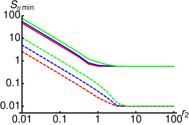
Figure 11: (Color online) The active/active interferometer with realistic photodetection. The plot shows the sensitivity $S_{\eta\,\mathrm{min}}$ as a function of $r_{2}$, for values of $N_{\mathrm{tot}}$ equal to $1$ (solid lines), and $100$ (dashed lines), and values of $\eta$ equal to $1$ (red lines), $0.6$ (blue line) and $0.2$ (green ones).

From the plot we obtain that the sensitivity $S_{\eta}$ is minimized when $r_{2}\gg 1$, independently of the value of $N_{\mathrm{tot}}$ and $\eta$. In particular, we find that the sensitivity is equal to the ideal sensitivity for $r_{2}\gg 1$. Therefore, if we pump into the system a large amount of energy with the second amplifier, we balance the losses of detectors, and are back to the ideal case. This result is analogue to that obtained in sect. V.2 for the passive interferometer with active measurement stage.

Since the sensitivity becomes equal to the ideal one for $r_{2}\gg 1$, the results of the previous section still hold. In particular, we have Heisenberg scaling in the high-energy regime, even if the detectors are affected by a non-unit quantum efficiency.

VI Features of the active measurement stage

The interferometers with active measurement stage shows a particular feature: the sensitivity $S_{\eta}$ in the presence of non unit quantum efficiency can be made equal to the ideal value $S_{1}$, by pumping a large number of squeezed photons inside the system with the OPA. In the following we further investigate this effect.

We consider the active measurement scheme, where the detectors have the same quantum efficiency $\eta$. The state of the modes $a$ and $b$ just before the active measurement stage is described by a generic state $\rho_{\phi}$, where $\phi$ is the phase parameter we want to estimate. Using the Heisenberg picture, the operator $D_{+}(\eta)$ associated with the sum photocurrent (after the OPA) can be written as (we assume, without loss of generality, that the OPA squeezing parameter $\xi$ is real):

$$D_{+}(\eta)=\eta\big{[}(1 +N_{\rm OPA})\langle N_{\rm in}\rangle_{\rho_{\phi}}+N_{\rm OPA}$$

$$+\sqrt{N_{\rm OPA}(2+N_{\rm OPA})}\langle X_{ab}\rangle_{\rho_{\phi}}\big{]}$$ (29)

where $\langle\cdots\rangle_{\rho_{\phi}}={\rm Tr}[\cdots\,\rho_{\phi}]$, $N_{\rm in}=a^{\dagger}a+b^{\dagger}b$, $X_{ab}=a^{\dagger}b^{\dagger}+ab$ and $N_{\mathrm{OPA}}=2\sinh^{2}\xi$ is the number of squeezed photons introduced with the amplifier. It is easy to show that:

$$\Delta D_{+}^{2}(\eta)=\eta^{2}\,\Delta D_{+}^{2}+\eta(1-\eta)\,D_{+}$$ (30)

where $D_{+}\equiv D_{+}(1)$ and the corresponding variance reads:

$$\Delta D_{+}^{2}=\ \langle D_{+}^{2}\rangle_{\rho_{\phi}}-\langle D_{+}\rangle_{\rho_{\phi}}^{2}$$

$$=\ (1+N_{\rm OPA})^{2}\Delta N_{\rm in}^{2}+N_{\rm OPA}(2+N_{\rm OPA})\Delta X_{ab}^{2}$$

$$+2(1+N_{\rm OPA})\sqrt{N_{\rm OPA}(2+N_{\rm OPA})}$$

$$\times\left(\frac{\langle N_{\rm in}X_{ab}+X_{ab}N_{\rm in}\rangle_{\rho_{\phi}}}{2}-\langle N_{\rm in}\rangle_{\rho_{\phi}}\langle X_{ab}\rangle_{\rho_{\phi}}\right).$$ (31)

The sensitivity $S_{\eta}$ for this measurement stage can be evaluated with the Eq. (14), and it is equal to

$$S_{\eta}=\ \frac{\sqrt{\Delta D_{+}^{2}(\eta)}}{\left|\partial_{\phi}D_{+}(\eta)\right|},$$ (32)

$$=\ S_{1}\sqrt{1+\frac{1-\eta}{\eta}\,\frac{D_{+}}{\Delta D_{+}^{2}}}\,.$$ (33)

Since $D_{+}/\Delta D_{+}^{2}\propto N_{\rm OPA}^{-1}$, it is now evident that, in the limit $\eta N_{\mathrm{OPA}}\gg 1$, one has $S_{\eta}\approx S_{1}$. We stress that this is a completely general result, since we are not making any assumption on the nature of the state $\rho_{\phi}$.

VII Concluding remarks

In this paper we have investigated the performances of optical interferometers involving Gaussian input signals and passive or active devices in the mixing stage as well as in the detection stage. For all the configurations we found the optimal working point of the interferometer by optimizing over all the involved parameters, either characterizing the interferometer or its input signals.

Upon analyzing the behaviour of the QFI, we have shown that both passive and active interferometers may achieve the Heisenberg scaling $\propto N_{\rm tot}^{-1}$ for a suitably optimized input signals in the high-energy regime, with the passive ones performing slightly better (by a multiplicative factor). In fact, the passive interferometer can fully exploit the squeezing resource whereas, in the case of the active one, part of the squeezing is lost to create entanglement between the two outgoing beams leading to a loss of local phase sensitivity. Our results also show that in order to achieve the ultimate limit allowed by quantum mechanics one should require that one of the two beams plays the role of a phase reference which is indeed enhanced by the use of squeezing.

We then moved to the realistic scenario in which we have a measurement stage based on passive or active elements and photon number detectors, taking also into account the presence of losses leading to a non-unit quantum efficiency. Our analytical and numerical results have shown that in the presence of unit quantum efficiency the symmetric configuration should be preferred: a passive (active) interferometer should use a passive (active) detection scheme. As one may expect, when losses affect the detection, the Heisenberg scaling is lost. However, we found that for both the passive and active interferometers the presence of an OPA at the measurement stage pumping a large number of squeezed photons allows to compensate the detrimental effect of losses and to achieve the same sensitivity as in the ideal casey, thus restoring again the Heisenberg scaling.

Our results show the robustness of Gaussian interferometers against loss, suggesting that their performances in realistic conditions may overcome those of the corresponding schemes involving finite superposition of photonic states raf1 ; raf2 , at least when synchronization is allowed between the sender and the receiver.

Appendix A Sum and difference photocurrent for non unit quantum efficiency

Here we address the first statistical moments of the sum- and the difference-photocurrent observables when the photodetectors have a non-unit quantum efficiency $\eta$. We model each realistic photodetector as an ideal one preceded by a beam splitter of transmissivity $\eta$, with the ancillary mode placed in the vacuum, see Fig. (12).

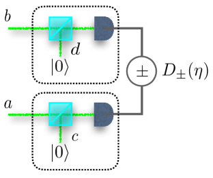
Figure 12: Sum and difference photocurrents $D_{+}(\eta)$ and $D_{-}(\eta)$ with realistic photodetectors. Here, we use a beam splitter with transmission coefficient $\eta$ to model quantum efficiency of detectors. Since a beam splitter has two input modes, one is filled with the radiation signal (the modes $``a"$ and $``b"$, in the scheme), while in the other (that is, the modes $``c"$ and $``d"$) we put a vacuum state $\left|{0}\right\rangle$.

The first operator we consider is the sum photocurrent. After straightforward calculation, both the mean value and the variance of this observable can be evaluated. The mean value is given by the equation

$$\langle D_{+}(\eta)\rangle=\eta\,\langle a^{\dagger}a+b^{\dagger}b\rangle$$ (34)

In other words, the mean value of the sum photocurrent is equal to the total number of photons inside the signal, scaled by the quantum efficiency of the detectors. Instead, the variance of this observable is given by

$$\langle\Delta D^{2}_{+}(\eta)\rangle= \>\eta^{2}\,\Big{(}\langle\Delta(a^{\dagger}a)^{2}\rangle+\langle\Delta(b^{\dagger}b)^{2}\rangle$$

$$+2\;\langle a^{\dagger}a\otimes b^{\dagger}b\rangle-2\;\langle a^{\dagger}a\rangle\langle b^{\dagger}b\rangle\Big{)}$$

$$+\eta(1-\eta)\,\langle a^{\dagger}a+b^{\dagger}b\rangle$$ (35)

The other observable we consider is the difference photocurrent $D_{-}(\eta)$. Its mean value is given by

$$\langle D_{-}(\eta)\rangle=\eta\,\langle a^{\dagger}a-b^{\dagger}b\rangle$$ (36)

In this case, the mean value of $D_{-}(\eta)$ is the difference between the number of photons collected by the two photodetectors. Again, the whole expression is scaled by $\eta$. In conclusion, the variance of the difference photocurrent can be evaluated

$$\langle\Delta D^{2}_{-}(\eta)\rangle= \>\eta^{2}\,\Big{(}\langle\Delta(a^{\dagger}a)^{2}\rangle+\langle\Delta(b^{\dagger}b)^{2}\rangle$$

$$-2\;\langle a^{\dagger}a\otimes b^{\dagger}b\rangle+2\;\langle a^{\dagger}a\rangle\langle b^{\dagger}b\rangle\Big{)}$$

$$+\eta(1-\eta)\,\langle a^{\dagger}a+b^{\dagger}b\rangle$$ (37)

In the equations from Eq. (34) to Eq. (A), the brackets $\langle\ldots\rangle$ represent the mean value on the state $\rho$ coming from the interferometer, that is to say, $\langle\ldots\rangle=\mathrm{Tr}\left[{\rho\,\ldots}\right]$.

References

- (1) R. Demkowicz-Dobrzański, M. Jarzyna, and J. Kołodyński, “Quantum Limits in Optical Interferometry”, Progress in Optics 60, 345 (2015).
- (2) H. Lee, P. Kok, J. P. Dowling, “A quantum Rosetta stone for interferometry”, J. Mod. Opt. 49, 2325 (2002).
- (3) J. Abadie, et al. (the LIGO Scientific Collaboration), “A gravitational wave observatory operating beyond the quantum shot-noise limit”, Nat. Phys. 7, 962 (2011).
- (4) R. Demkowicz-Dobrzański, K. Banaszek, and R. Schnabel, “Fundamental quantum interferometry bound for the squeezed-light-enhanced gravitational wave detector GEO 600”, Phys. Rev. A 88, 041802(R) (2013).
- (5) A. A. Berni, T. Gehring, B. M. Nielsen, V. Handchen, M. G. A. Paris, and U.L. Andersen, “Ab-initio Quantum Enhanced Optical Phase Estimation Using Real-time Feedback Control”, Nature Phot. 9, 577 (2015).
- (6) M. Hillery, L. Mlodinow, “Interferometers and minimum-uncertainty states”, Phys. Rev. A 48, 1548 (1993).
- (7) G. M. D’Ariano, M. G. A. Paris, “Lower bounds on phase sensitivity in ideal and feasible detection schemes”, Phys. Rev. A 49, 3022, (1994).
- (8) M. G. A. Paris, “Small amount of squeezing in high-sensitive realistic interferometry”, Phys. Lett A 201, 132 (1995).
- (9) T. Kim, Y. Ha, J. Shin, H. Kim, G. Park, K. Kim, T.-G. Noh, and C. K. Hong, “Effect of the detector efficiency on the phase sensitivity in a Mach-Zehnder interferometer”, Phys. Rev. A 60, 708 (1999).
- (10) S. Olivares, and M. G. A. Paris, “Optimized Interferometry with Gaussian States”, Optics Spectr. 103, 231 (2007).
- (11) L. Pezzé, and A. Smerzi,, “Mach-Zehnder interferometry at the heisenberg limit with coherent and squeezed-vacuum light”, phys. rev. lett. 100, 073601 (2008).
- (12) B. Yurke, S. L. McCall, and J. R. Klauder, “SU(2) and SU(1,1) interferometers”, Phys Rev. A 33, 4033 (1986).
- (13) A. M. Marino, N. V. Corzo Trejo, and P. D. Lett, “Effect of losses on the performance of an SU(1,1) interferometer”, Phys. Rev. A 86, 023844 (2012).
- (14) Sh. Barzanjeh, D. P. DiVincenzo, and B. M. Terhal “Dispersive qubit measurement by interferometry with parametric amplifiers”, Phys. Rev. B 90, 134515 (2014).
- (15) T. Kim, H. Kim, “Phase sensitivity of a quantum Mach-Zehnder interferometer for a coherent state input”,J. Opt. Soc. Am. B 26, 671 (2009).
- (16) W. N. Plick, J. P. Dowling, and G. S. Agarwal, “Coherent-light-boosted, sub-shot noise, quantum interferometry”, New J. Phys. 12, 083014 (2010).
- (17) J. Jing, C. Liu, Z. Zhou, F. Hudelist, C. Yuan, L. Chen, X, Li, J. Qian, K. Zhang, L. Zhou, Lu, H. Ma, G. Dong, Z. Ou, W. Zhang, “Squeezing bandwidth controllable twin beam light and phase sensitive nonlinear interferometer based on atomic ensembles”, Chin. Phys. Bull. 57, 1925 (2012).
- (18) F. Hudelist, J. Kong, C. Liu, J. Jing, Z.Y. Ou, W. Zhang, “Quantum metrology with parametric amplifier-based photon correlation interferometers”, Nat. Comm. 5, 3049 (2014)
- (19) S. Sparaciari, S. Olivares, and M. G. A. Paris, “Bounds to precision for quantum interferometry with Gaussian states and operations”, J. Opt. Soc. Am. B 32, 1354 (2015).
- (20) M. G. A. Paris, “Quantum estimation for quantum technology”, Int. J. Quant. Inf. 7, 125 (2009).
- (21) U. Leonhardt, H. Paul, “Realistic optical homodyne measurements and quasiprobability distributions” Phys. Rev. A 48, 4598 (1993).
- (22) C. Vitelli, N. Spagnolo, L. Toffoli, F. Sciarrino, F. De Martini, “Enhanced resolution of lossy interferometry by coherent amplification of single photons”, Phys. Rev. Lett. 105, 113602 (2010)
- (23) C. W. Helstrom, Quantum Detection and Estimation Theory (Academic Press, New York, 1976).
- (24) D. C. Brody, and L. P. Hughston, “Statistical geometry in quantum mechanics”, Proc. Roy. Soc. Lond. A 454, 2445 (1998); “Geometrization of statistical mechanics”, Proc. Roy. Soc. Lond. A 455, 1683 (1999).
- (25) S. L. Braunstein, and C. M. Caves, “Statistical distance and the geometry of quantum states”, Phys. Rev. Lett. 72, 3439 (1994).
- (26) S. L. Braunstein, C. M. Caves, and G. J. Milburn, “Generalized uncertainty relations: Theory, examples, and Lorentz invariance”, Ann. Phys. 247, 135 (1996).
- (27) Z. Jiang, “Quantum Fisher information for states in exponential form”, Phys. Rev. A 89, 032128 (2014).
- (28) A. Monras, “Phase space formalism for quantum estimation of Gaussian states”, arXiv:1303.3682 [quant-ph].
- (29) O. Pinel, P. Jian, N. Treps, C. Fabre, and D. Braun, “Quantum parameter estimation using general single-mode Gaussian states”, Phys. Rev. A 88, 040102(R) (2013).
- (30) D. D. de Souza, M. G. Genoni, and M.S. Kim, “Continuous-variable phase estimation with unitary and random linear disturbance”, Phys. Rev. A 90, 042119 (2014).
- (31) L. Banchi, S. L. Braunstein, S. Pirandola, “Quantum fidelity for arbitrary Gaussian states”, preprint arXiv:1507.01941
- (32) S. Olivares, “Quantum optics in the phase space”, Eur. Phys. J. ST 203, 3 (2012).
- (33) S. Olivares, and M. G. A. Paris, “Fidelity Matters: The Birth of Entanglement in the Mixing of Gaussian States”, Phys. Rev. Lett 107, 170505 (2011).
- (34) M. D. Lang, and C. M. Caves, “Optimal Quantum-Enhanced Interferometry Using a Laser Power Source” Phys. Rev. Lett. 111, 173601 (2013).
- (35) M. D. Lang, and C. M. Caves, “Optimal quantum-enhanced interferometry”, Phys. Rev. A 90, 025802 (2014).
- (36) R. Demkowicz-Dobrzanski, U. Dorner, B. J. Smith, J. S. Lundeen, W. Wasilewski, K. Banaszek, I. A. Walmsley, “Quantum phase estimation with lossy interferometers”, Phys. Rev. A 80, 013825 (2009).
- (37) M. Kacprowicz, R. Demkowicz-Dobrzanski, W. Wasilewski, K. Banaszek and I. A. Walmsley, “Experimental quantum-enhanced estimation of a lossy phase shift”, Nature Phot. 4, 357 (2010).