Hydrogen-Water Mixtures in Giant Planet Interiors Studied with Ab Initio Simulations

Abstract

We study water-hydrogen mixtures under planetary interior conditions using ab initio molecular dynamics simulations. We determine the thermodynamic properties of various water-hydrogen mixing ratios at temperatures of 2000 and 6000 K for pressures of a few tens of GPa. These conditions are relevant for ice giant planets and for the outer envelope of the gas giants. We find that at 2000 K the mixture is in a molecular regime, while at 6000 K the dissociation of hydrogen and water is important and affects the thermodynamic properties. We study the structure of the liquid and analyze the radial distribution function. We provide estimates for the transport properties, diffusion and viscosity, based on autocorrelation functions. We obtained viscosity estimates of the order of a few tenths of mPa s for the conditions under consideration. These results are relevant for dynamo simulations of ice giant planets.

Keywords:

hydrogen, water, planetary interior, transport properties.

1 Introduction

The extraordinary discovery of more than one thousand confirmed exoplanets in the past decade [1] underlines the necessity for a better description of their structure, formation, and evolution. The discovery of an unexpectedly rich population of Neptune and Sub-Neptune exoplanets [2] stressed the need for a better understanding of these kinds of planets. Based on the gravitational moments measured by Voyager II and orbital observations of their satellites [3, 4], different models have been proposed for the two ice giants of our solar system, Uranus and Neptune [5, 6]. Still, considerable uncertainties about their internal composition remain, and a more accurate equations of state (EOS) is needed to improve the models.

Furthermore, magnetic field observations provide additional information and add some constraints on interior models. Dynamo simulations [7, 8, 9] predicted that water in different phases is important for the magnetic field generation. So far, such dynamo simulations rely on ice giant interior models that assume water to be fully phase separated from other compounds including hydrogen. Recent ab initio computer simulations predicted that water and metallic hydrogen readily mix at pressure-temperature conditions in the cores of giant planets. Experimental data obtained at lower pressures [10] predicted the true picture to be more complex and suggested partial mixing of water and hydrogen. These results may also become relevant for the interiors of gaseous giant planets like Saturn and Jupiter because the presence of a small amount of water would affect the physical properties of their envelopes. The properties of hydrogen-water mixtures in different concentrations are thus of significant interest in planetary science.

Here we performed computer simulations of fluid water-hydrogen mixtures at different concentrations under the pressure-temperature conditions found in Neptune’s and Uranus’ upper mantle and the outer envelope of Jupiter and Saturn. We explored the effects of the concentration, temperature, and pressure on both the thermodynamic properties and the structure of the fluid. The most significant changes are introduced when the hydrogen and water dissociate at high temperature and pressure. We also computed the transport properties, such as particle diffusion and viscosity in order to better constrain the dynamo simulations.

2 Simulation method

We performed molecular dynamics simulations based on finite temperature density functional theory (DFT) using the Vienna Ab initio Simulation Package (VASP) [11]. We studied four different mixtures from H₂O:H₂=16:64, 24:48, 32:32, and 40:16 molecules in simulation cell. We define the water concentration as $x=N_{\textrm{H}_{2}\textrm{O}}/(N_{\textrm{H}_{2}\textrm{O}}+N_{\textrm{H}_{2}})$.

Simulation results for pure water and hydrogen can be found in Refs. [12, 13, 14] and [15, 16, 17, 18, 19]. Our simulations were at least 3 ps long for a time-step of 0.2 fs, short enough to accurately describe the H-H and O-H bonds vibrations. The temperature was kept constant using a Nosé thermostat [20, 21].

The electronic structure was computed at each time step using Mermin’s finite temperature approach [22] of the Kohn-Sham scheme [23], with a Fermi-Dirac occupation distribution. We used projector augmented wave (PAW) pseudopotentials [24] with a cut-off radius of $r_{\textrm{cut}}=0.8~{}a_{0}$ for hydrogen and $r_{\textrm{cut}}=1.1~{}a_{0}$ for oxygen. For the plane-wave basis, an energy cut-off of $1100$ eV was needed to reach a convergence with less than 1% inaccuracy on both the energy and the pressure. We used the generalized gradient approximation (GGA) with the Perdew, Burke, and Ernzerhof (PBE) [25] exchange-correlation functional that gave reasonable results in similar systems [26, 12]. All simulations were performed using periodic boundary conditions. We chose to use the Baldereschi k-point [27] for sampling the Brillouin zone because it gave similar thermodynamic functions (within 1%) to a 2$\times$2$\times$2 Monkhorst-Pack grid [28].

In this article we will present results at two temperatures: 2000 and 6000 K with pressures ranging from 10$-$35 GPa and 10$-$70 GPa for the lower and higher temperatures, respectively. These conditions are close to what we find in Neptune’s or Uranus’ upper mantle [29, 30, 6] or in the outer envelop of Jupiter and Saturn [31, 32].

3 Results and discussion

3.1 Thermodynamic properties

We extracted the pressure and the internal energy time-averages from the different molecular dynamics simulations. The error bars presented in the figures were computed using the block averaging method [33]. In Fig. 1, we report the evolution of the molecular density as a function of the pressure at 2000 K. The trend is quite similar for each mixing ratio. Molecular densities are much higher for hydrogen-rich mixtures, which simply reflects the fact the hydrogen molecules are smaller than the water molecules.

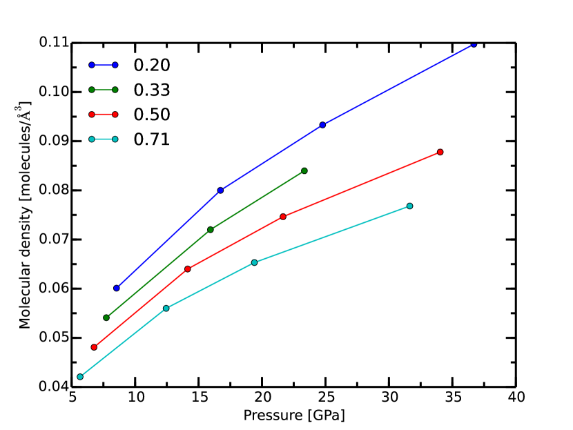
Figure 1: (color online) Molecular density as a function of the pressure at 2000 K. The four colors are for the four different H₂O concentrations, $x$, given in the caption.

In Fig. 2, we plotted the internal energy per molecule as function of pressure for two temperatures. The curves for each concentration have been shifted in order to superpose them for each isotherm and compare their evolution as a function of the pressure.

At 2000 K, the linear behavior of the energy is very similar for all concentrations, indicating that the thermal excitations of H₂ and H₂O molecules make similar contributions to both the internal energy and the pressure. In contrast, we find significant deviations from the linear relationship at 6000 K. More importantly, there is a dependence on the concentration, indicating a change of structure of the liquid, which we discuss in section 3.2.

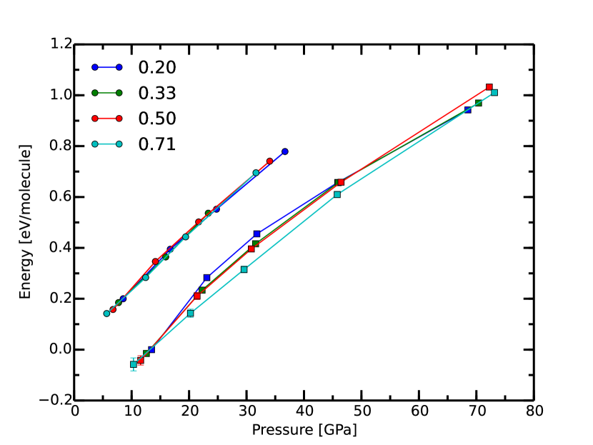
Figure 2: (color online) Internal energy per molecule as a function of the pressure at 2000 K ($\bullet$) and 6000 K ($\blacksquare$). The energies have been manually shifted for each concentration and temperature to better compare them as function of pressure. At 2000 K, the energy origins for each concentration have been chosen so that at 8.6 GPa, the energy is 0.2 eV/mol. For the 6000 K isotherm, the energy at 13.5 GPa is 0.0 eV/mol. The four colors are for the four different H₂O concentrations, $x$, given in the caption.

3.2 Structure and composition

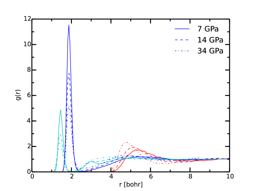
Figure 3: (color online) Radial distribution function of a $x=0.5$ mixture at 2000 K and different pressures. The O-O structure is plotted in red, O-H in blue and H-H in cyan.

The molecular dynamics simulations provide information about the microscopic structure of the fluid. Radial distribution functions (RDF) are an established tool [34, 35] to analyze the structure. A first example is shown in Fig. 3, where we plotted the RDF of an equimolar mixture, $x=0.5$, at three different pressures and a 2000 K temperature. The large peaks in the O-H and H-H correlations underline the molecular character of the fluid, which is fully molecular up to at least 35 GPa. There appear to be no other strong correlations in the fluid besides the molecular structure except at highest pressure where the correlation among the oxygen nuclei increases. Under these conditions, the fluid is close to phase transition to a superionic regime at 40-50 GPa at 2000 K in pure water [12].

In Fig. 4, we plotted the RDF for a $x=0.5$ mixture at 6000 K. The size of the H-H and H-O peaks is significantly reduced compared to 2000 K indicating a partial dissociation of the molecules. This dissociation is consistent with the behavior observed in pure hydrogen [26] and water [12]. We infer that the dissociation is the cause of the concentration dependence of the internal energy-pressure relationship in Fig. 2. We did not identify any other correlations besides the molecular peaks but it should be noted that the O-O correlation increases at 70 GPa.

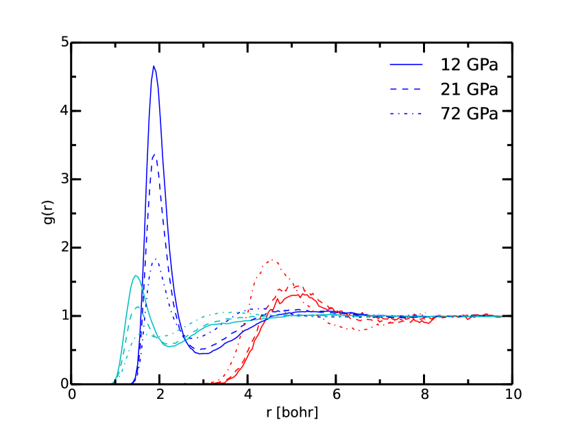
Figure 4: (color online) Radial distribution function of a $x=0.5$ mixture at 6000 K and different pressures. The O-O structure is plotted in red, O-H in blue and H-H in cyan.

3.3 Transport properties

3.3.1 Autocorrelation functions

We derived the viscosity and diffusion coefficients of the hydrogen and oxygen species in each mixture in order to provide some dynamic information about the mixture and ultimately to improve models for planetary interiors. We used the autocorrelation functions for the diffusion and viscosity calculations. The diffusion coefficient of species is given by the Green-Kubo formula [36, 34]:

$$D_{\alpha}=\frac{1}{3N_{\alpha}}\sum_{\alpha}\int_{0}^{+\infty}\langle\textbf{v}_{\alpha}(\tau)\cdot\textbf{v}_{\alpha}(0)\rangle\;\textrm{d}\tau,$$ (1)

where we sum over all $N_{\alpha}$ nuclei of type $\alpha$. $\textbf{v}_{\alpha}(\tau)$ is the particle’s velocity vector at time $\tau$. The brackets mean that we average over many possible time origins assuming the fluid has reached an equilibrium in our simulations[37]. To reduce the fluctuations further, we averaged the result from different maximum integration times ranging from 75 to 100% of our time-window. The error bars in Figures 5-6 and Tables 1-2 represent one standard deviation from the mean.

We computed the viscosity, $\eta$, from the autocorrelation function of the stress-tensor $\sigma_{\alpha\beta}$,

$$\eta=\frac{V}{3k_{\textrm{B}}T}\sum_{\{\alpha\beta\}}\int_{0}^{+\infty}\langle\sigma_{\alpha\beta}(\tau)\sigma_{\alpha\beta}(0)\rangle\;\textrm{d}\tau,$$ (2)

where the sum $\{\alpha\beta\}$ includes all the deviatoric stress tensor components, $\{xy,xz,yz\}$. $V$ is the volume of the simulation cell and $T$ the temperature of the system. There are still strong fluctuations in the stress tensor autocorrelation function even when we use multiple origins because the stress-tensor is a bulk property and it is not possible to average over the multiple particles. In order to reduce the spreads in the results we fitted the autocorrelation function by a simple exponential function. This method provides more stable estimates of the viscosity. Nevertheless, we do not provide error bars in the figures because our viscosity values have to be considered to be order-of-magnitude estimates only because it is too difficult to obtain an accurate determination of the viscosity and its error bar.

3.3.2 Diffusion

We analyze the diffusion of individual nuclei rather than tracking the motion of molecules because the latter method becomes difficult as soon as dissociation and recombination effects occur at elevated temperature.

Figure 5: (color online) Oxygen diffusion coefficient as a function of the pressure at 2000 K ($\bullet$) and 6000 K ($\blacksquare$).The four colors are for the four different H₂O concentrations, $x$, given in the caption.

In Fig. 5, we plotted the diffusion coefficient of oxygen nuclei as function of pressure for 2000 and 6000 K. For both temperatures, we find that diffusion slows down with increasing pressure because the particle interact more strongly. At 6000 K, the diffusion is faster because the additional kinetic energy allows particles to hop over potential barriers more rapidly. The oxygen diffusion rate decreases with increasing water concentration presumably because water molecules interact more strongly with each other than they do with hydrogen molecules at the same pressure.

The diffusion coefficient of the hydrogen nuclei are plotted in Fig. 6. For the dissociated fluids at 6000 K, the hydrogen atoms diffuse approximately twice as fast as the oxygen atoms that are heavier and larger. In the molecular regime, the hydrogen and oxygen diffusion rates are more similar because some hydrogen nuclei are bound to oxygen. Again we find that when the water concentration rises, the diffusion slows down. There is at least two reasons for that. First, an increasing fraction of hydrogen nuclei is bound in water molecules, which greatly restricts their mobility. Second the mobility of the hydrogen molecules is reduced by the interaction with water molecules.

It is interesting to note that the diffusion rates at 6000 K are almost independent of pressure. This is most likely due to two counter-acting effects. With increase pressure, particles interact more strongly, which reduces diffusion rates. A pressure increase also introduces a rise in the dissociation fraction, which increases the mobility of different nuclei.

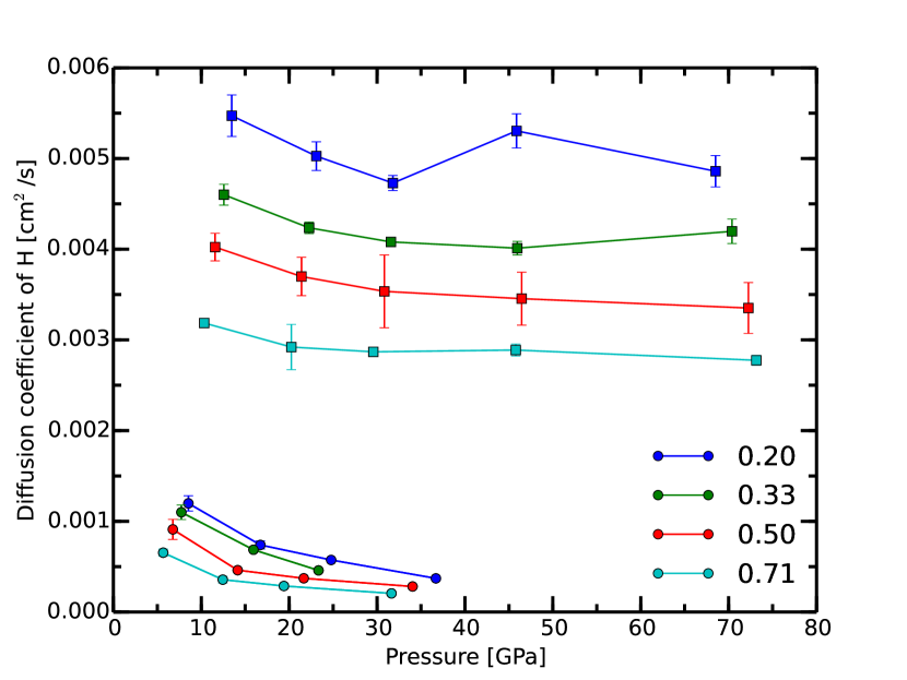
Figure 6: (color online) Hydrogen diffusion coefficient as a function of the pressure at 2000 K ($\bullet$) and 6000 K ($\blacksquare$). The four colors are for the four different H₂O concentrations, $x$, given in the caption.

3.3.3 Viscosity

In Fig. 7, we plotted our viscosity estimates for the H₂-H₂O mixtures. Values vary from 0.1 to 1 mPa s over the range of parameters that we explored here. The viscosity rises with increasing water concentration because water molecules interact more strongly than hydrogen molecules at the same pressure. The viscosity rises with increasing pressure and decreasing temperature, as expected. Viscosity estimates are of importance for the numerical simulations of planetary interiors, especially for Neptune-like planets where the water content is presumably high. Moreover, the viscosity plays a prominent role in the dynamics of the dynamo [7, 8, 9] and reliable estimates are therefore needed.

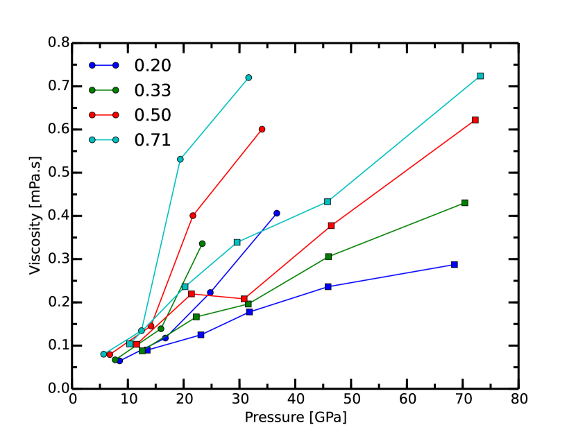
Figure 7: (color online) Viscosity as a function of the pressure at 2000 K ($\bullet$) and 6000 K ($\blacksquare$). The four colors are for the four different H₂O concentrations, $x$, given in the caption.

Table 1: Hydrogen and oxygen diffusion coefficients and pressure table for different molecular densities and water concentrations $x_{{\textrm{H}_{2}\textrm{O}}}$ at 2000 K.

$x_{{\textrm{H}_{2}\textrm{O}}}$	Mol. dens.	Pressure	H diffusion	O diffusion
	($\times 10^{-2}$Å$\!{}^{-3}$)	(GPa)	($\times 10^{-3}\!$ cm2/s)	($\times 10^{-3}\!$ cm2/s)
0.20	6.0105	8.534(36)	1.197(84)	0.876(30)
0.20	8.0000	16.73(11)	0.739(45)	0.441(80)
0.20	9.3308	24.776(45)	0.573(10)	0.377(22)
0.20	10.974	36.694(75)	0.371(23)	0.219(59)
0.33	5.4095	7.731(46)	1.099(80)	0.683(90)
0.33	7.2000	15.936(56)	0.686(14)	0.427(52)
0.33	8.3977	23.339(90)	0.459(16)	0.266(49)
0.50	4.8084	6.763(30)	0.91(11)	0.622(85)
0.50	6.4000	14.139(64)	0.461(19)	0.346(43)
0.50	7.4646	21.66(13)	0.371(15)	0.252(7)
0.50	8.7792	34.04(14)	0.281(12)	0.157(17)
0.71	4.2074	5.667(51)	0.654(39)	0.560(14)
0.71	5.6000	12.45(11)	0.357(38)	0.296(61)
0.71	6.5316	19.40(14)	0.287(32)	0.060(18)
0.71	7.6818	31.64(10)	0.205(23)	0.090(13)

Table 2: Same as Table 1 but at 6000 K.

$x_{{\textrm{H}_{2}\textrm{O}}}$	Mol. dens.	Pressure	H diffusion	O diffusion
	($\times 10^{-2}$Å$\!{}^{-3}$)	(GPa)	($\times 10^{-3}\!$ cm2/s)	($\times 10^{-3}\!$ cm2/s)
0.20	6.0105	13.47(11)	5.47(23)	2.54(12)
0.20	8.0000	23.09(11)	5.03(16)	1.67(46)
0.20	9.3308	31.80(12)	4.729(83)	1.834(72)
0.20	10.974	45.87(11)	5.30(19)	1.245(75)
0.20	13.027	68.514(96)	4.86(17)	1.190(64)
0.33	5.4095	12.57(12)	4.60(11)	2.11(18)
0.33	7.2000	22.26(11)	4.236(63)	1.39(13)
0.33	8.3977	31.581(93)	4.080(34)	1.12(24)
0.33	9.8765	45.95(16)	4.011(75)	1.01(13)
0.33	11.724	70.38(16)	4.20(13)	0.878(64)
0.50	4.8084	11.570(81)	4.02(15)	1.95(26)
0.50	6.4000	21.40(18)	3.70(21)	1.388(56)
0.50	7.4646	30.83(15)	3.54(40)	1.05(11)
0.50	8.7792	46.45(16)	3.46(29)	0.931(85)
0.50	10.421	72.25(16)	3.35(28)	0.616(51)
0.71	4.2074	10.32(11)	3.186(32)	1.76(10)
0.71	5.6000	20.24(17)	2.92(25)	1.132(48)
0.71	6.5316	29.57(16)	2.869(50)	0.87(17)
0.71	7.6818	45.78(19)	2.888(67)	0.568(72)
0.71	9.1187	73.14(23)	2.775(54)	0.491(38)

4 Conclusion

We performed ab initio computer simulations of H₂-H₂O mixtures at 2000 K and 6000 K in order to provide information about the physics of such systems under conditions in the interior of icy or gaseous giant planets. We showed for instance that at 2000 K and a few tens of GPa, the mixture is purely molecular and its thermodynamic behavior depends only weakly on the water concentration. In contrast, at 6000 K we observe partial dissociation of both H₂ and H₂O molecules, which changes in the thermodynamic behavior. Because dissociation is often associated with a reduction in the electronic band gap, we can infer that the dissociated fluids [38] have a significantly higher electronic conductivity. This has potential implications for the magnetic field generation in water-rich gas giants planets.

The autocorrelation function analysis provided robust results for the diffusion of oxygen and hydrogen nuclei in the mixtures. The diffusion of hydrogen is almost constant at 6000 K from 10 to 70 GPa range due to the dissociation process that add to the mobility of the protons. The diffusion coefficients are important for the planetary models because the diffusion influences the convective behavior in the semi-convective regime as shown by Leconte and Chabrier [31]. We also computed the viscosity which is of the order of a few tenths of mPa s at the conditions under consideration. This is not a very viscous fluid indicating a turbulent behavior in planetary interiors.

5 Acknoledgements

This work has been supported by NSF and NASA. The simulations were performed on the NASA supercomputing facilities.

References

References

- nas [????] Exoplanet Archive, URL http://exoplanetarchive.ipac.caltech.edu, ????
- Petigura et al. [2013] E. A. Petigura, G. W. Marcy, A. W. Howard, A Plateau in the Planet Population below Twice the Size of Earth, Astrophys. J. 770 69.
- Jacobson [2007] R. A. Jacobson, The gravity field of the Uranian system and the orbits of the Uranian satellites and rings, Bulletin of the American Astronomical Society 39 (2007) 453.
- Jacobson [2009] R. A. Jacobson, The orbits of the Neptunian satellites and the orientation of the pole of Neptune, Astrophys. J. 137 (2009) 4322.
- Helled et al. [2011] R. Helled, J. D. Anderson, M. Podolak, G. Schubert, Interiors Models of Uranus and Neptune, Astrophys. J. 726 (2011) 15.
- Nettelmann et al. [2013] N. Nettelmann, R. Helled, J. Fortney, R. Redmer, New indication for a dichotomy in the interior structure of Uranus and Neptune from the application of modified shape and rotation data, Planetary and Space Science 77 (0) (2013) 143 – 151.
- Stanley and Bloxham [2004] S. Stanley, J. Bloxham, Convective-region geometry as teh cause of Uranus’ and Neptune’s magnetic fields, Nature 428 (2004) 151.
- Stanley and Bloxham [2006] S. Stanley, J. Bloxham, Numerical dynamo models of Uranus’ and Neptune’s unusual magnetic fields, Icarus 184 (2006) 556.
- Bloxham et al. [2013] J. M. Bloxham, M. H. Heimpel, E. M. King, J. M. Aumou, Turfields models of ice giant internal dynamics: Dynamos, heat transfer, and zonal flows, Icarus 224 (2013) 97.
- Bali et al. [2013] E. Bali, A. Audétat, H. Keppler, Waplanet hydrogen are immiscible in Earth’s mantle, Nature 495 (2013) 220.
- vas [????] Vienna Ab initio Simulation Package, URL http://www.vasp.at, ????
- French et al. [2009] M. French, T. R. Mattsson, N. Nettelmann, R. Redmer, Equation of state and phase diagram of water at ultrahigh pressures as in planetary interiors, Phys. Rev. B 79 (2009) 054107, URL http://link.aps.org/doi/10.1103/PhysRevB.79.054107.
- Wilson et al. [2013] H. F. Wilson, M. L. Wong, B. Militzer, Phys. Rev. Lett. 110 (2013) 151102.
- P21 [????] B. Militzer, S. Zhang, ”Ab initio Simulations of Superionic H2O, H2O2, and H9O4 Compounds”, submitted to Phys. Rev. B (2014), ????
- Militzer and Ceperley [2000] B. Militzer, D. M. Ceperley, Phys. Rev. Lett. 85 (2000) 1890.
- Militzer and Ceperley [2001] B. Militzer, D. M. Ceperley, Phys. Rev. E 63 (2001) 066404.
- Vorberger et al. [2007] J. Vorberger, I. Tamblyn, B. Militzer, S. Bonev, Phys. Rev. B 75 (2007) 024206.
- Militzer [2013] B. Militzer, Phys. Rev. B 87 (2013) 014202.
- Militzer and Hubbard [2013] B. Militzer, W. B. Hubbard, Astrophys. J. 774 (2013) 148.
- Nosé [1984] S. Nosé, J. Chem. Phys 81 (1984) 511.
- Nosé [1991] Nosé, Prog. Theor. Phys. Suppl. 103 (1991) 1.
- Mermin [1965] N. D. Mermin, Thermal Properties of the Inhomogeneous Electron Gas, Phys. Rev. 137 (5A) (1965) A1441–A1443.
- Kohn and Sham [1965] W. Kohn, L. J. Sham, Self-Consistent Equations Including Exchange and Correlation Effects, Physical Review 140 (1965) 1133.
- Blöchl [1994] P. E. Blöchl, Projector augmented-wave method, Phys. Rev. B 50 (24) (1994) 17953–17979.
- Perdew et al. [1996] J. P. Perdew, K. Burke, M. Ernzerhof, Generalized Gradient Approximation Made Simple, Phys. Rev. Lett. 77 (18) (1996) 3865–3868.
- Caillabet et al. [2011] L. Caillabet, S. Mazevet, P. Loubeyre, Multiphase equation of state of hydrogen from ab initio calculations in the range 0.2 to 5 g/cc up to 10 eV, Phys. Rev. B 83 (2011) 094101, URL http://link.aps.org/doi/10.1103/PhysRevB.83.094101.
- Baldereschi [1973] A. Baldereschi, Mean-Value Point in the Brillouin Zone, Phys. Rev. B 7 (1973) 5212–5215, URL http://link.aps.org/doi/10.1103/PhysRevB.7.5212.
- Monkhorst and Pack [1976] H. J. Monkhorst, J. D. Pack, Special points for Brillouin-zone integrations, Phys. Rev. B 13 (12) (1976) 5188.
- Hubbard et al. [1991] W. B. Hubbard, W. J. Nellis, A. C. Mitchell, N. C. Holmes, P. C. McCandless, S. S. Limaye, Interior structure of Neptune - Comparison with Uranus, Science 253 (1991) 648–651.
- Podolak et al. [1995] M. Podolak, A. Weizman, M. Marley, Comparative models of Uranus and Neptune, Planet. Space Sci. 43 (1995) 1517–1522.
- Leconte and Chabrier [2012] J. Leconte, G. Chabrier, A new vision of giant planet interiors: Impact of double diffusive convection, A&A 540 A20.
- Militzer et al. [2008] B. Militzer, W. H. Hubbard, J. Vorberger, I. Tamblyn, S. A. Bonev, Astrophys. J. Lett. 688 (2008) L45.
- Rapaport [2004] D. C. Rapaport, The Art of Molecular Dynamics Simulation, Cambridge University Press, 2004.
- Frenkel and Smit [2002] D. Frenkel, B. Smit, Understanding molecular simulation: from algorithms to applications, Academic Press, 2002.
- Hansen and McDonald [1986] J.-P. Hansen, I. McDonald, Theory of simple liquids, Academic Press, second edn., 1986.
- Danel et al. [2012] J.-F. Danel, L. Kazandjian, G. Zérah, Numerical convergence of the self-diffusion coefficient and viscosity obtained with Thomas-Fermi-Dirac molecular dynamics, Phys. Rev. E 85 (2012) 066701.
- Haile [1997] J. M. Haile, Molecular Dynamics Simulation, Wiley-Interscience, 1997.
- Collins et al. [2001] L. A. Collins, S. R. Bickham, J. D. Kress, S. Mazevet, T. J. Lenosky, N. J. Troullier, W. Windl, Dynamical and optical properties of warm dense hydrogen, Phys. Rev. B 63 (2001) 184110.