Entanglement Entropy and Topological Order in Resonating Valence-Bond Quantum Spin Liquids

Abstract

On the triangular and kagome lattices, short-ranged resonating valence bond (RVB) wave functions can be sampled without the sign problem using a recently-developed Pfaffian Monte Carlo scheme. In this paper, we study the Renyi entanglement entropy in these wave functions using a replica-trick method. Using various spatial bipartitions, including the Levin-Wen construction, our finite-size scaled Renyi entropy gives a topological contribution consistent with $\gamma=\text{ln}(2)$, as expected for a gapped $\mathbb{Z}_{2}$ quantum spin liquid. We prove that the mutual statistics are consistent with the toric code anyon model and rule out any other quasiparticle statistics such as the double semion model.

Introduction. – Two-dimensional frustrated quantum antiferromagnets can harbor a phase of matter called a quantum spin liquid; a state with no conventional symmetry but emergent, topological order Wen (1990, 2013). These phases are unique in that they exhibit gapped fractionalized quasiparticle excitations with exotic quantum statistics and ground state degeneracies on topologically non-trivial surfaces Balents (2010). Although there is strong incentive to identify minimal theoretical models which possess topologically ordered phases, the fact that strong correlations are a crucial ingredient means that numerical methods necessarily play a large role. Numerical studies suffer several serious challenges. First, the vast majority of Hamiltonians and wave functions that may harbor candidate quantum spin liquid states are also afflicted with the “sign problem”, precluding study by large-scale quantum Monte Carlo (QMC) Kaul et al. (2013). Also, the absence of a local order parameter in a quantum spin liquid means that topological order must be characterized through more refined techniques, such as universal scaling terms in the entanglement entropy - the topological entanglement entropy (TEE) $-\gamma$ Levin and Wen (2006); Kitaev and Preskill (2006). Since $\gamma$ is sub-leading to the diverging “area-law”, it can be challenging to extract in numerical simulations Isakov et al. (2011); Zhang et al. (2011); Grover et al. (2013); Zhu et al. (2014). Finally, distinct topological phases defined by different emergent quasiparticles can have the same TEE. To distinguish, one must rely on the modular $\mathcal{U}$ and $\mathcal{S}$-matrices, which encode information on the quasiparticle statistics of the underlying topological phase Zhang et al. (2012); Cincio and Vidal (2013).

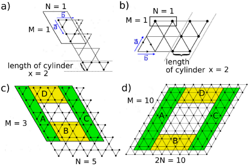
Figure 1: a) The 6-site unit cell of the kagome lattice and the phase convention for singlets living on the lattice links. The length of the cylindrical regions that the entanglement entropy $S_{2}$ is measured over is shown as $x$. b) The 2-site unit cell, the respective phase convention and the definition of $x$ for the triangular lattice. c) and d) show the Levin-Wen areas $A,B,C$ and $D$ for the kagome lattice of size $(M,N)=(3,5)$ amounting to $90$ sites, and the $10\times 10$-triangular lattice, respectively. The TEE $-\gamma$ is obtained by a superposition of the EE of four areas: $-2\gamma=S_{ABCD}-S_{ABC}-S_{ADC}+S_{AC}$.

In this Letter, we analyze the Renyi entanglement entropy of the short-ranged spin-$\frac{1}{2}$ resonating valence bond (RVB) wave function on the kagome and the triangular lattice. Recently Ref. Wildeboer and Seidel (2012) introduced a sign-problem free Pfaffian Monte Carlo scheme that can be used to produce unbiased samples of the singlet wave function, making it possible to evaluate local operators and their correlation functions. That work demonstrated that the RVB wave function on these two frustrated lattices has no local order parameter, and is gapped, consistent with expectations for an $SU(2)$-invariant quantum spin liquid. Here, we use the Pfaffian Monte Carlo technique to calculate the TEE, which explicitly shows $\gamma=\text{ln}(2)$, as expected for a $\mathbb{Z}_{2}$ topologically-ordered phase. Further, we prove that the mutual statistics are consistent with the toric code anyon model in both the triangular and kagome RVB states, ruling out any other underlying anyon models such as the double semion.

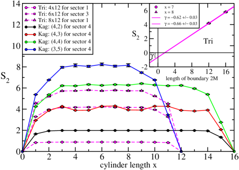
Figure 2: The Renyi entropy $S_{2}$ for triangular (Tri) lattices of size $M\times 2N=4,6,8\times 12$ and kagome (Kag) lattices for various sizes $(M,N)$ with total number of lattice sites $6MN$. There are four possible topological sectors for each wave function on a torus, each of which can be isolated independently in the Pfaffian MC. For the triangular lattice, the inset shows linear fits using $S_{2}$ from $M\times 2N=6,8\times 12$ for lengths $x=7,8$ in order to extract $\gamma^{\prime}$ for a single sector. In total, we average over values stemming from fits for $4\leq x\leq 8$, and obtain an average value of $-\gamma^{\prime}=-0.64\pm 0.07$.

RVB Wave Functions, Entanglement, and QMC. – The RVB wave functions were conceived by Anderson 40 years ago Anderson (1973) for their variational appeal in demonstrating spin liquid physics. The simplest, nearest-neighbor RVB state represents a stable phase only on non-bipartite lattices. Although not typically discussed as ground states of explicit local Hamiltonians, RVB wave functions do sometimes allow for the construction of a local parent Hamiltonian, as notable in particular on the kagome lattice Seidel (2009). The uniqueness of the RVB-ground states, modulo a topological degeneracy, (demonstrated in Refs. Schuch et al. (2010); Zhou et al. (2014)) establishes that the Hamiltonian in Ref. Seidel (2009) truly stabilizes the RVB state. In this work, we will directly consider the RVB wave function, defined via

$$|RVB\rangle=\sum_{D}|D\rangle\,.$$ (1)

Here, $D$ goes over all possible pairings of a given lattice into nearest neighbor pairs (“dimer coverings”). Each site of the lattice is equipped with a spin-$\frac{1}{2}$ degree of freedom. For each dimer covering $D$, $|D\rangle$ denotes a state where each pair of lattice sites of the covering forms a singlet, where a sign convention is used that corresponds to an orientation of nearest neighbor links (see Fig. 1a & b). We note that the wave function Eq. (1) has a fourfold topological degeneracy on the torus for the kagome and triangular lattices.

Like in any quantum wave function, the properties of an RVB state can be investigated through its bipartite entanglement entropy, where the lattice is divided into a region $A$ and its complement $B$. The Renyi entropy of order $n$ is defined as $S_{n}=\text{ln Tr}(\rho_{A}^{n})/(1-n)$, where $\rho_{A}=\text{Tr}_{B}|\Psi\rangle\langle\Psi|$ is the reduced density matrix of region $A$. Ground states of local Hamiltonians are known to exhibit a area law scaling in region size, which in two dimensions can generically be written as, $S_{n}(\rho_{A})=\alpha_{n}L_{A}-\gamma+\cdots$ Eisert et al. (2010). Here, the leading term is dependent on the “area” (or boundary) of region $A$. The second term, the topological entanglement entropy (TEE) $-\gamma$ Levin and Wen (2006); Kitaev and Preskill (2006), is characterized by the total quantum dimension $\mathcal{D}$, which is defined through the quantum dimensions of the individual quasiparticles $d_{i}$ of the underlying theory: $\mathcal{D}=\sqrt{\sum_{i}d_{i}^{2}}$ Levin and Wen (2006); Kitaev and Preskill (2006); Dong et al. (2008). Conventionally ordered phases have $\mathcal{D}=1$, while topologically ordered phases have $\mathcal{D}>1$ with the TEE given by $-\gamma=-\text{ln}(\mathcal{D})$.

Note that in the case where the area $A$ has at least one non-contractible boundary, such as a cylinder (see Fig. 1a & b), $\gamma$ becomes state-dependent. As shown in Ref. Zhang et al. (2012), if one expresses any state in the basis of the minimum entropy states (MES-states), $|\Psi_{\alpha}\rangle=\sum_{j}c_{j}|\Xi_{j}\rangle$, then the sub-leading constant to the area law from a two-cylinder cut is,

$$\gamma^{\prime}(\{p_{j}\})=2\gamma+\text{ln}\bigg{(}\sum_{j}\frac{p_{j}^{2}}{d_{j}^{2}}\bigg{)}\;.$$ (2)

for $S_{2}$, where $p_{j}=|c_{j}|^{2}$. We further discuss MES-states in the results to follow.

In contrast to bipartite lattices Sutherland (1988); Liang et al. (1988); Sandvik (2005); Albuquerque and Alet (2010); Tang et al. (2011); Ju et al. (2012); Stéphan et al. (2013); Punk et al. (2015), RVB states on non-bipartite lattices are not amenable to valence-bond QMC; they have been studied previously by PEPs representations Verstraete et al. (2006); Schuch et al. (2012); Iqbal et al. (2014), but should also be accessible to QMC if a sign-problem free sampling method can be constructed Becca et al. (2011); Yang and Yao (2012); Wildeboer and Seidel (2012). Here, we investigate entanglement properties of the spin-$\frac{1}{2}$ RVB wave functions using the variational Pfaffian MC scheme for lattices of up to $128$ sites. Note that the Pfaffian MC scheme allows one to project onto each topological sector, and every linear combination thereof. We will use this feature in the following results. To obtain the second Renyi entropy $S_{2}$ for contractible and noncontractible regions, we employ the standard QMC replica-trick Hastings et al. (2010); Kallin et al. (2011). We refer to Refs. SM ; Wildeboer and Seidel (2012) for more details on the method.

Measurements of TEE. – We begin by calculating the TEE using boundaries for region $A$ that are contractible around the toroidal lattice. To isolate $\gamma$, we perform a Levin-Wen bipartition Levin and Wen (2006), which was successfully used previously to detect a $\mathbb{Z}_{2}$ quantum spin liquid using QMC simulations on toroidal lattices of restricted finite-size Isakov et al. (2011). We obtain data for such bipartitions on both a triangular RVB of size $M\times 2N=10\times 10$ and two kagome RVBs with $(M,N)=(3,5),(3,6)$ amounting to $90$ and $108$ sites, respectively. The triangular lattice and the $(3,5)$-kagome geometries are shown in Fig. 1, which also shows the Levin-Wen regions $A,B,C,D$ used to obtain $\gamma$ Levin and Wen (2006). For the $(3,6)$-kagome, the $A(C)$ regions are the same as in $(3,5)$, whereas the regions $B(D)$ are one link longer in $N$-direction than in $(3,5)$. Using this procedure, the triangular lattice gives $-\gamma\approx-0.80\pm 0.2$, while for the kagome, we end up with $-\gamma=-0.89\pm 0.22,-0.74\pm 0.34$ for $(3,5)$ and $(3,6)$, respectively.

To improve accuracy, we now consider regions with non-contractible boundaries. We examine a triangular lattice RVB for fixed $2N=12$ and $M=4,6,8$, and a kagome lattice RVB of size $6MN$ with $M=4$ and $N=2,3,4$. We subsequently calculate the Renyi entropy $S_{2}$ for cylindrical bipartitions (see Fig. 1). As the cylinder length increases, $S_{2}$ quickly saturates (Fig. 2). This type of behavior is consistent with the system having a gap. We point out that, as expected, several curves in Fig. 2 exhibit finite size effects, manifest clearly in the different $S_{2}$ for different topological sectors. This can be seen in Fig. 3, 7 and 8 SM .

Figures 3 and 7 demonstrate that, for large enough system sizes, $S_{2}$ does not depend on the topological sector for these two wave functions. The four topological sectors $|\Psi_{i}\rangle$ of each wave function can be distinguished by their two quantum numbers, $i=\{ee,eo,oe,oo\}$, which are the even $(e)$ or odd $(o)$ number of dimers cut along the two directions $\vec{a}$ and $\vec{b}$. One can make use of special linear combinations of these topological sectors to devise another method of determining the TEE $-\gamma$. Here, we choose as a compatible ansatz for $\mathbb{Z}_{2}$ spin liquids the minimal-entangled states (MES) obtained for the toric code and the dimer model on kagome/triangular lattices Zhang et al. (2012); SM and examine its properties. These MES-states for cuts along $\vec{b}$ are, up to a phase $e^{i\Phi_{j}}$,

$$|\Xi_{1,2}\rangle=\frac{1}{\sqrt{2}}(|\Psi_{ee}\rangle\pm|\Psi_{eo}\rangle)\;,$$

$$|\Xi_{3,4}\rangle=\frac{1}{\sqrt{2}}(|\Psi_{oe}\rangle\pm|\Psi_{oo}\rangle)\;.$$ (3)

We apply this ansatz to our Pfaffian QMC data. First, consider slices (of constant cylinder length $x$) through the triangular lattice to obtain a plot of $S_{2}(L_{2M})=\alpha L_{2M}-\gamma^{\prime}$, as in the inset of Fig. 2. The intercept of this plot is $-\gamma^{\prime}$ which is now the state dependent TEE; we numerically extract $-\gamma^{\prime}=-0.64\pm 0.07$. We can thus obtain the TEE using Eq. (2). First note that, as seen in Fig. 7 of the SM, the entropy $S_{2}$ does not depend on which MES-state is used (within error bars), which implies that $d_{j}$ is also the same for all four MES-states. Since every theory, Abelian and non-Abelian, contains (at least) one quasiparticle with quantum dimension unity, we conclude that all quasiparticle dimensions are necessarily $d_{j}=1$. Since the $p_{j}$ are fixed to be $1/4$ by our ansatz Eq. (Entanglement Entropy and Topological Order in Resonating Valence-Bond Quantum Spin Liquids), then for the single sector plotted in Fig. 2, $\gamma^{\prime}=2\gamma+\text{ln}({1}/{4}+{1}/{4})$. Thus, we conclude that $\gamma=0.67\pm 0.04$ consistent with $\mathbb{Z}_{2}$ topological order.

Next we turn to the kagome lattice RVB. As seen in Fig. 3 (inset) and Fig. $8$ in the SM SM , it takes a system of size $(M,N)=(4,3)$ to eliminate finite-size effects and reach agreement of $S_{2}$ of all four topological sectors within error bars. Since larger system sizes can become computationally expensive, an extraction of $\gamma^{\prime}$ using the procedure of Fig. 2 becomes more difficult. Alternatively, as discussed in Ref. Zhang et al. (2012), linear superpositions of different MES states can be used to extract all information about the topological order from our measurement. Specifically, the linear combination of all four MES-states,

$$|\Sigma_{1,2}\rangle=\frac{1}{\sqrt{2}}(|\Psi_{ee}\rangle+|\Psi_{oe(oo)}\rangle)$$

$$=\frac{1}{2}\bigg{(}|\Xi_{1}\rangle+|\Xi_{2}\rangle+|\Xi_{3}\rangle\pm|\Xi_{4}\rangle\bigg{)},$$ (4)

will have $\gamma^{\prime}=0$ according to Eq. (2). Here, index $1$ ($2$) corresponds to $oe$ ($oo$), and $+$ ($-$) in the second line.

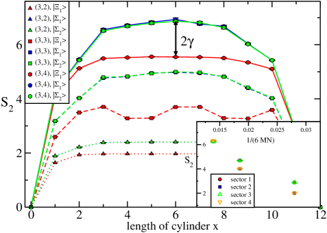
Figure 3: $S_{2}$ for kagome-lattice MES-state $(|\Xi_{1}\rangle)$ which is a specific superposition of two topological sectors for different lattice sizes and for two respective nonMES-states $(|\Sigma_{1,2}\rangle)$. The difference between $(M,N)=(3,4)$ for the two nonMES-states compared to the MES-state has to be $2\gamma=2\text{ln}(2)\approx 1.38$. If we average over differences obtained for lengths $x=5,6,7$, we get $-\gamma^{\prime}=-2\gamma=-1.36\pm 0.13$. The inset shows a comparison of $S_{2}$ for cylindrical regions between sectors $1,2,3,4$ on the kagome lattice. We observe that for large enough system sizes $(M,N)=(3,4)$ amounting to $72$ lattice sites, the EE $S_{2}$ is the same for all four sectors within errors.

We investigate the behavior of $S_{2}$ for the MES-state, Eq. (Entanglement Entropy and Topological Order in Resonating Valence-Bond Quantum Spin Liquids), and the nonMES-states, Eq. (Entanglement Entropy and Topological Order in Resonating Valence-Bond Quantum Spin Liquids), for the kagome lattice RVB. We first note that the numerical data of Fig. 3 (Figs. $7,8$ in the SM) suggests $S_{2}$ to be independent of MES-state (once finite-size effects are accounted for). Since $S_{2}$ is similarly the same across all four topological sectors, this implies that $\gamma^{\prime}$ is the same for all $|\Xi_{i}\rangle$ and for all $|\Psi_{i}\rangle$, respectively. The latter means that each of the four quasi-particles belonging to the four MES-states have the same quantum dimension. Since every phase, Abelian and non-Abelian, has (at least) one quasi-particle with quantum dimension $d=1$, this implies that all quasi-particles have $d_{i}=1$, indicating the Abelian nature of the phase. We calculate the difference in $S_{2}$ between MES (Entanglement Entropy and Topological Order in Resonating Valence-Bond Quantum Spin Liquids) and nonMES (Entanglement Entropy and Topological Order in Resonating Valence-Bond Quantum Spin Liquids) states by performing an average over cylinder lengths $x=4,\ldots,8$, and obtain $-\gamma^{\prime}=-1.36\pm 0.13$. This matches the expectation from Eq. (2) that this difference should be $-2\gamma\approx-1.38$, confirming that the MES ansatz is also correct for the kagome-lattice RVB.

Quasiparticle Statistics. – We point out that the numerical confirmation of the MES-states ansatz Eq. (Entanglement Entropy and Topological Order in Resonating Valence-Bond Quantum Spin Liquids) essentially determines the topological order of our system, and in particular distinguishes between toric code and double semion topological order as we now explain. We consider the matrices $\mathcal{S}$ and $\mathcal{U}$, which describe the quasiparticle statistics of the system and correspond to modular transformations of the same name at the level of the effective field theory. In a microscopic lattice model, the corresponding transformations cannot necessarily be realized as discrete symmetry operations. However, for both the kagome and the triangular lattice, the transformation corresponding to $\mathcal{U}\mathcal{S}^{-1}$ is realized as the symmetry under a $\pi/3$-rotation SM , as long as the lattice dimensions are chosen to be of the form $(M,N)=(M,2M)$ or $(M,2N)=(2N,2N)$ for the kagome or triangular, respectively. Up to a phase ambiguity Zhang et al. (2012), the matrix elements $V_{ij}=\langle\Xi_{i}|R_{\pi/3}|\Xi_{j}\rangle$ are thus equal to those of the matrix $\mathcal{US}^{-1}$, where $R_{\pi/3}$ represents the $\pi/3$-rotation. We therefore must have $V_{ij}=D^{\dagger}\mathcal{US}^{-1}D$, where $D$ is a diagonal matrix of phases $D_{jj}=e^{i\Phi_{j}}$ corresponding to the phase ambiguity. $V_{ij}$ is easily calculated from Eq. (Entanglement Entropy and Topological Order in Resonating Valence-Bond Quantum Spin Liquids) by working out the transformation properties of the states $|\Psi_{\alpha,\beta}\rangle$ under rotation Poilblanc and Misguich (2011); SM . It is manifestly real, as is $\mathcal{US}^{-1}$ for the toric code, and we find agreement for $D_{jj}=1$ for all $jj$’s. In contrast, for the double semion model, $\mathcal{US}^{-1}$, while having the same eigenvalues as in the toric code case, we note that $\mathcal{U}$ has some purely imaginary diagonal entries. Therefore, in the double semion case, $D^{\dagger}\mathcal{US}^{-1}D$ must have imaginary entries for any choice of $D$, and agreement with our MES-states cannot be achieved.

Thus, the MES-states we identified demonstrate the underlying quasiparticle statistics to be consistent with the toric code model, ruling out any other statistics, in particular double semion statistics.

Conclusion. – In this work, we have used a sign-problem free Pfaffian quantum Monte Carlo (QMC) to calculate the second Renyi entropy of the nearest-neighbor RVB wave function on the triangular and kagome lattices. Through a bipartition of each lattice into Levin-Wen Levin and Wen (2006) regions, and cylindrical regions, we confirm that the topological entanglement entropy (TEE) is consistent with $-\gamma=-\text{ln}(2)$, the value for a $\mathbb{Z}_{2}$ quantum spin liquid. Finite-size scaling of the two-cylinder Renyi entropy for the triangular lattice and comparisons between $S_{2}$ for different wave functions in MES-basis for the kagome, confirm the ansatz MES-states taken for a $\mathbb{Z}_{2}$ topological gauge structure. Further, we identify the nature of the anyonic quasiparticles to be of toric code type, by explicitly showing that our numerically confirmed MES-states ansatz leads to the modular $\mathcal{US}^{-1}$-matrix of the toric code statistics and rules out any other quasiparticle statistics including double semion statistics.

This work serves as an important example that all aspects of quantum spin liquid behavior, from the initial demonstration of the liquid nature Wildeboer and Seidel (2012) to the characterization of the emergent gauge structure through the TEE, to the full determination of the underlying statistics and braiding of fractional quasiparticle excitations, can be performed with un-biased QMC techniques. Thus, the $SU(2)$-invariant RVB states on triangular and kagome lattices add to the growing list of wave functions and Hamiltonians that have been demonstrated to exist, and can be simulated in practice, on non-bipartite lattices without being vexed by the sign-problem Kaul et al. (2013); Kaul (2015).

Finally, we emphasize that our results rely crucially on the numerical extraction of the second Renyi entropy of the quantum ground state. For RVB wave functions (and all other many-body systems), the replica-trick method used here Hastings et al. (2010) is the same as that employed in recent experiments on interacting ⁸⁷Rb atoms in a one-dimensional optical lattice Islam et al. (2015). Hence, the concepts and techniques used in this paper will be important for efforts to characterize topological order in synthetic quantum matter in the near future.

Supplemental material: Entanglement Entropy and Topological Order in Resonating Valence-Bond Quantum Spin Liquids

Julia Wildeboer

Alexander Seidel

Roger G. Melko

1) The Kasteleyn method for the triangular lattice. – The close-packed hard-core dimer model can be solved on any planar lattice by using Pfaffian techniques Kasteleyn (1963). The key ingredient for the Pfaffian technique is to place arrows on the links of the planar graph/lattice so that each plaquette is “clockwise odd”, that is to say that the product of the orientations of the arrows around any even-length elementary plaquette traversed clockwise is odd. Subsequently, an antisymmetric matrix $A$ is formed.

Kasteleyn’s theorem then states that for any planar graph, $A$ can be found, and that the partition function which is the number of dimer coverings NNo is given by the Pfaffian of the matrix $A$:

$$Z=\pm{\rm Pf}(A)\;.$$ (5)

However, (5) is only valid for a system with open boundary conditions (OBC). If we work on a toroidal system, we will see that we need a total of four Pfaffians.

Thus, we start by defining the four matrices $A_{i}$, $i=1,2,3,4$ in case of the toroidal triangular lattice. The adopted Kasteleyn edge orientation and the unit cell of the triangular lattice containing $2$ sites, numbered $1$ and $2$, respectively, are shown in Fig. 4. In the following, we consider a lattice of $M\times N$ unit cells having a total of $M\times 2N$ lattice sites, the case of $M=3,2N=4$ is shown in Fig. 4.

The Pfaffian method Kasteleyn (1963) concerns with the evaluation of the $2MN\times 2MN$ antisymmetric Kasteleyn matrices $A$ written down according to edge weights and orientations (under specific boundary conditions) which can be read off from Fig. 4, and by adopting the prescription

$$A_{ij}=\left\{\begin{array}[]{lr}+w_{ij}&{\rm orientation\ from\ }i{\rm\ to\ }j\\ -w_{ij}&{\rm orientation\ from\ }j{\rm\ to\ }i\end{array}\right.$$ (8)

where $w_{ij}$ is the weight of edge $ij$. In the following, we take all edge weights $w_{ij}=1$.

KasteleynKasteleyn (1963) has shown that under periodic boundary conditions (PBC) the partition function $Z_{torus}$ is a linear combination of four Pfaffians Pf$(A_{i}),i=1,\ldots,4$,

$$Z_{torus}=\frac{1}{2}\Big{[}-{\rm Pf}(A_{1})+{\rm Pf}(A_{2})+{\rm Pf}(A_{3})+{\rm Pf}(A_{4})\Big{]}.$$ (9)

The four Pfaffians are specified by the Kasteleyn orientation of lattice edges with, or without, the reversal of arrows on edges connecting two opposite boundaries. A perusal of Fig. 4 and the use of the prescription (8) lead to the four $2MN\times 2MN$ Kasteleyn matrices,

$$\begin{split}A_{1}=&a_{0,0}\otimes I_{M}\otimes I_{N}+a_{0,1}\otimes I_{M}\otimes T_{N}-a_{0,1}^{T}\otimes I_{M}\otimes T_{N}^{T}\\ &+a_{1,0}\otimes T_{M}\otimes I_{N}-a_{1,0}^{T}\otimes T_{M}^{T}\otimes I_{N}\\ &+a_{1,1}\otimes T_{M}\otimes T_{N}^{T}-a_{1,1}^{T}\otimes T_{M}^{T}\otimes T_{N}\\ A_{2}=&a_{0,0}\otimes I_{M}\otimes I_{N}+a_{0,1}\otimes I_{M}\otimes H_{N}-a_{0,1}^{T}\otimes I_{M}\otimes H_{N}^{T}\\ &+a_{1,0}\otimes T_{M}\otimes I_{N}-a_{1,0}^{T}\otimes T_{M}^{T}\otimes I_{N}\\ &+a_{1,1}\otimes T_{M}\otimes H_{N}^{T}-a_{1,1}^{T}\otimes T_{M}^{T}\otimes H_{N}\\ A_{3}=&a_{0,0}\otimes I_{M}\otimes I_{N}+a_{0,1}\otimes I_{M}\otimes T_{N}-a_{0,1}^{T}\otimes I_{M}\otimes T_{N}^{T}\\ &+a_{1,0}\otimes H_{M}\otimes I_{N}-a_{1,0}^{T}\otimes H_{M}^{T}\otimes I_{N}\\ &+a_{1,1}\otimes H_{M}\otimes T_{N}^{T}-a_{1,1}^{T}\otimes H_{M}^{T}\otimes T_{N}\\ A_{4}=&a_{0,0}\otimes I_{M}\otimes I_{N}+a_{0,1}\otimes I_{M}\otimes H_{N}-a_{0,1}^{T}\otimes I_{M}\otimes H_{N}^{T}\\ &+a_{1,0}\otimes H_{M}\otimes I_{N}-a_{1,0}^{T}\otimes H_{M}^{T}\otimes I_{N}\\ &+a_{1,1}\otimes H_{M}\otimes H_{N}^{T}-a_{1,1}^{T}\otimes H_{M}^{T}\otimes H_{N}.\end{split}$$ (10)

The superscripts $T$ denote transpose, $\otimes$ is the direct product, $I_{M}$ is the $M\times M$ identity matrix, and $H_{N}$, $T_{N}$ are the $N\times N$ matrices

$$H_{N}=\begin{pmatrix}0&1&0&\cdots&0\\ 0&0&1&\cdots&0\\ \vdots&\vdots&\vdots&\ddots&\vdots\\ 0&0&0&\cdots&1\\ -1&0&0&\cdots&0\end{pmatrix},\quad T_{N}=\begin{pmatrix}0&1&0&\cdots&0\\ 0&0&1&\cdots&0\\ \vdots&\vdots&\vdots&\ddots&\vdots\\ 0&0&0&\cdots&1\\ 1&0&0&\cdots&0\end{pmatrix}.$$ (11)

and

$$a_{0,0} = \begin{pmatrix}\;\;\;0&1\cr-1&0\cr\end{pmatrix},\quad a_{0,1}=\begin{pmatrix}0&0\cr 1&0\cr\end{pmatrix},$$

$$a_{1,0} = \begin{pmatrix}-1&0\cr\;\;\;1&1\cr\end{pmatrix},\quad a_{1,1}=\begin{pmatrix}0&-1\cr 0&\;\;\;0\cr\end{pmatrix},$$ (12)

$$a_{-1,0} = -a_{1,0}^{T},\quad a_{0,-1}=-a_{0,1}^{T},\quad a_{-1,-1}=-a_{1,1}^{T}.$$

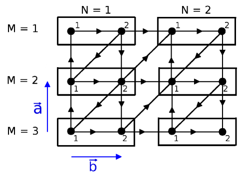
Figure 4: Shown is a triangular lattice with $M\times 2N=3\times 4=12$ sites with a Kasteleyn edge orientation. The unit cell consists of two lattice sites labeled 1 and 2, respectively.

The need for four matrices is explained in the following.

class of configurations	sign of terms in ${\rm Pf}(A_{i})$
	$\;\;A_{1}\;\;$	$\;\;A_{2}\;\;$	$\;\;A_{3}\;\;$	$\;\;A_{4}\;\;$
sector $1$: $(e,e)$	+	+	+	+
sector $2$: $(o,e)$	-	-	+	+
sector $3$: $(e,o)$	-	+	-	+
sector $4$: $(o,o)$	-	+	+	-

Table 1: The counting rules for the dimer coverings belonging to the four sectors $(ee)$, $(eo)$, $(oe)$, $(oo)$.

The single dimer coverings fall into four sectors that are distinguished by the even ($e$) or odd ($o$) number of dimer cuts of a loop along the two directions $\vec{a}$ and $\vec{b}$ of the torus. Each of the four Pfaffians only counts one or three types of the four sectors $(ee)$, $(eo)$, $(oe)$, $(oo)$, correctly (see Table  1). However, if we form the superposition (9), then all dimer coverings from all four sectors are counted with the correct sign. It is now also possible to project onto each sector:

$$Z_{1} = \frac{1}{4}({\rm Pf}(A_{1})-{\rm Pf}(A_{2})-{\rm Pf}(A_{3})-{\rm Pf}(A_{4}))$$

$$Z_{2} = \frac{1}{4}(-{\rm Pf}(A_{1})-{\rm Pf}(A_{2})+{\rm Pf}(A_{3})+{\rm Pf}(A_{4}))$$

$$Z_{3} = \frac{1}{4}(-{\rm Pf}(A_{1})+{\rm Pf}(A_{2})-{\rm Pf}(A_{3})+{\rm Pf}(A_{4}))$$

$$Z_{4} = \frac{1}{4}(-{\rm Pf}(A_{1})+{\rm Pf}(A_{2})+{\rm Pf}(A_{3})-{\rm Pf}(A_{4}))\;.$$

The partition sum for open boundary conditions can be obtained by taking any of the matrices $A_{i}$, $i=1,\ldots,4$, and setting the links in the $M(N)\times M(N)$ matrices that connect sites from opposite boundaries equal to zero.

$M$	$N$	$2MN$	$Z_{torus}$	$Z_{1}$	$Z_{2}$	$Z_{3}$	$Z_{4}$
3	2	12	344	92	80	92	80
4	2	16	1920	576	448	448	448
5	2	20	10608	2872	2432	2872	2432
6	2	24	59040	16720	12592	15696	14032
3	3	18	4480	1120	1120	1120	1120
4	3	24	59040	16720	15696	12592	14032
5	3	30	767776	191824	192064	191824	192064
3	4	24	58592	14576	14720	14576	14720
4	4	32	1826944	520256	512064	389184	405440
3	5	30	766528	191200	192064	191200	192064
3	6	36	10028288	2505344	2508800	2505344	2508800

Table 2: Number of dimer coverings, $Z_{torus}$, of triangular lattices of with $2MN$ sites, with periodic boundary conditions. $Z_{i}$ gives the number of coverings for each topological sector $i$ with $i=1,\ldots,4$. Only those sizes ($M\geq 3$ and $N\geq 2$) are given in which any pair of sites is linked by at most one bond.

To close this section, we remark that the analogous Pfaffian construction for the kagome lattice is available in Ref.Wu and Wang (2008) by Wu and Wang. Here, the unit cell consists of a total of $6$ lattice sites, the total number of sites is then $6MN$ (see Fig. $1$ in Letter). An analytic calculation reveals the full partition sum to be $Z_{torus}=2\times 4^{MN}$.

Eventually, we give Tables  2 and  3 that list the full partition sum $Z_{torus}$ and the sector-wise partition sums $Z_{i}$, ($i=1,\ldots,4$), for small lattice sizes for the triangular and the kagome lattice. For the kagome lattice, the single sectors have the feature that they exactly have the same number of dimer coverings, $Z_{i}=\frac{1}{2}\times 4^{MN}$, for all pairs $(M,N)$ for $i=1,\ldots,4$.

For the triangular lattice, we observe that in general different lattice sizes lead to different number of dimer coverings in the single sectors. However, it is possible to have $\frac{1}{4}Z_{torus}$ coverings in each sector for certain pairs $(M,N)$, one example being $(M,N)=(3,3)$ with $\frac{1}{4}Z_{torus}=1120$ dimer coverings per sector.

$M$	$N$	$6MN$	$Z_{torus}$	$Z_{i}(i=1,\ldots,4)$
1	2	12	32	8
2	2	24	512	128
2	3	36	8192	2048
2	4	48	131072	32768
2	5	60	2097152	524288
3	2	36	8192	2048
3	3	54	524888	131072
3	4	72	33554432	8388608
3	5	90	2147483648	536870912
3	6	108	137438953472	34359738368
4	2	48	131072	32768
4	3	72	33554432	8388608
4	4	96	8589934592	2147483648
4	5	120	2199023255552	549755813888

Table 3: Number of dimer coverings, $Z_{torus}$, of kagome lattices of with $6MN$ sites, with periodic boundary conditions. $Z_{i}$ gives the number of coverings for each topological sector $i$ with $i=1,\ldots,4$.

2) Entanglement and SWAP-operator for the RVB wave function. – We start by briefly reviewing the variational Pfaffian Monte Carlo scheme introduced in Ref.Wildeboer and Seidel (2012). The scheme was introduced to overcome a sign problem that prevents the application of the valence bond Monte Carlo (VBMC) technique to the short-ranged RVB wave function on the non-bipartite kagome and triangular lattices. Only for bipartite lattices it is possible to endow each link of the lattice with a sign/phase convention that renders all overlaps between different singlet coverings positive. This has to be so, since the overlaps serve as weights in the VBMC. For non-bipartite lattices, such as the kagome and the triangular lattice, there exists no such sign convention.

The idea is now the re-express the RVB wave function in a orthogonal basis, which does not suffer from a sign problem, rather than the non-orthogonal valence bond basis of Eq. (1).

First, we re-cast the RVB wave function (1) in terms of the Ising basis of local $S^{z}$ eigenstates. For a system consisting of an even number $N$ of spins/sites, we thus re-express Eq. (1) as:

$$|\text{RVB}\rangle=\sum_{I}a_{I}|I\rangle,$$ (14)

where $|I\rangle=|m_{1}^{z}\rangle\otimes|m_{2}^{z}\rangle\otimes\ldots\otimes|m_{N}^{z}\rangle$ runs over the Ising basis. The newly appearing non-trivial amplitude $a_{I}$ can easily be calculated as the Pfaffian of an $N\times N$ matrix. This Pfaffian can be re-expressed as a $N/2\times N/2$-determinant which can be evaluated in polynomial time.

We point out that our state $|\Psi\rangle$ given as in (14) is actually the sum over all four topological sectors: $|\Psi\rangle=\sum_{i=1}^{4}|\Psi_{i}\rangle$. We stress that we are able to restrict the sum in the state $|\Psi\rangle$ to any sector through a calculation of four specific Pfaffians (see Section $1)$). Subsequently, we are able to project onto any topological sector and onto any linear combinations of sectors when sampling the RVB wave function. More details on this issue are given in Kasteleyn (1963); Wildeboer and Seidel (2012) and in Section $1)$.

Next, we adapt the standard QMC replica trick, the so-called SWAP-trick, and apply it to (14) in order to calculate the Renyi entropy.

The Renyi entropy of order $n$ is defined as

$$S_{n}=\frac{1}{1-n}\text{ln}\,\text{Tr}(\rho_{A}^{n})\;.$$ (15)

In the limit $n\rightarrow 1$, the von Neumann entropy is recovered. The TEE $-\gamma$ does not depend on $n$.

Since it is computationally expensive to calculate the von Neumann entropy, we proceed by calculating the second Renyi entropy. Here, the well-known QMC replica trick allows us to avoid the costly calculation of the reduced density matrix $\rho_{A}$ which is needed for the von Neumann entropy and to alternatively efficiently calculate the second Renyi entropy by obtaining the expectation value of the so-called SWAP-operator Hastings et al. (2010); Kallin et al. (2011).

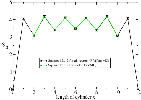
Figure 5: SQUARE: The EE $S_{2}$ over a cylindrical area $A$ is shown for the $12\times 12$-square lattice. We do not observe any differences within error bars between $S_{2}$ for a specific sector and when calculated with the sum over all sectors. The “all-sector”-data was obtained by Pfaffian Monte Carlo, while the “single-sector”-data stems from a VBMC simulation.

Using the SWAP-operator, calculating the second Renyi entropy over an area $A$ requires us to make two independent copies of the system, the total state of the doubled system is then $|\Psi\otimes\Psi^{\prime}\rangle=\sum_{II^{\prime}}a_{I}a_{I^{\prime}}|I\otimes I^{\prime}\rangle$ The SWAP-operator now exchanges the degrees of freedom in area $A$ between the two copies while leaving the degrees of freedom in the remaining area $B$ untouched:

$$\text{SWAP}|I_{A}I_{B}\otimes I_{A}^{\prime}I_{B}^{\prime}\rangle=|I_{A}^{\prime}I_{B}\otimes I_{A}I_{B}^{\prime}\rangle\;.$$ (16)

It can be shown that $\langle\text{SWAP}\rangle=\text{Tr}(\rho_{A}^{2})$ Hastings et al. (2010) and consequently

$$S_{2}=-\text{ln}(\langle\text{SWAP}\rangle)\;.$$ (17)

Using the RVB wave function (14) for calculating the expectation value $\langle\text{SWAP}\rangle$, we arrive at the following:

$$\langle\text{SWAP}\rangle=\frac{\sum_{II^{\prime}}|a_{I}|^{2}|a_{I^{\prime}}|^{2}\;\times\;R}{\sum_{II^{\prime}}|a_{I}|^{2}|a_{I^{\prime}}|^{2}}$$ (18)

with the measurement/estimator

$$R=\frac{a_{I^{s}}a_{I^{\prime,s}}}{a_{I}a_{I^{\prime}}}\;,$$ (19)

where $I^{s}$ and $I^{\prime,s}$ refer to the Ising configurations of system and its copy after the SWAP-operation.

It is clear from (18) and (19) that the measurement depends on the state of the two systems after the exchange of the degree of freedoms.

Since the number of Ising configurations grows exponentially with the size of the subsystem $A$, we have exponentially large fluctuations in the estimator $R$ and as it is implied by the area law, the convergence of the entanglement entropy becomes exponentially slow. Only an exponentially small part of the original Ising configuration will lead to a non-zero measurement of $R$. Most measurements will be zero. Thus, in order to combat the exponentially growing variance of the simple estimator $R$ in (19), we employ a more refined re-weighting scheme from Ref.Pei et al. (2014). The new re-weighting scheme splits the expectation value $\langle\text{SWAP}\rangle$ into two parts

$$\langle\text{SWAP}\rangle=\langle\text{SWAP}_{sign}\rangle\times\prod_{i}^{m}\langle\text{SWAP}_{amp}\rangle_{i}\;.$$ (20)

The first part is the sign-dependent part of the SWAP-operator, the second part is itself a product over all contributions to the amplitude of SWAP. We find for the sign-dependent part:

$$\langle\text{SWAP}_{sign}\rangle = \frac{\sum_{II^{\prime}}|A(I,I^{\prime},I^{s},I^{\prime,s})|e^{i\Phi(I,I^{\prime})}}{\sum_{I,I{\prime}}|A(I,I^{\prime},I^{s},I^{\prime,s})|}$$

where we defined the weight

$$W(I,I^{\prime})=|A(I,I^{\prime},I^{s},I^{\prime,s})| = |a_{I}a_{I^{\prime}}a_{I^{s}}a_{I^{\prime,s}}|$$

and $\Phi(I,I^{\prime})$ is the phase of $R$. The RVB wave function is real, thus, we have $e^{i\Phi(I,I^{\prime})}=\pm 1$.

The amplitude-dependent part itself is a product. This allows us to express the quantity $\langle\text{SWAP}_{amp}\rangle$ to be evaluated as the product of a series of ratios so that the evaluation of each ratio only suffers from a much smaller fluctuation. This can practically be done be introducing $r_{i}\in[0,1]$ as a series of powers satisfying $r_{i}<r_{i+1}$, $r_{1}=0$ and $r_{m+1}=1$. Defining the weight

$$\tilde{W}_{i}(I,I^{\prime}) = |A(I,I^{\prime},I^{s},I^{\prime,s})|^{1-r_{i+1}}\times\Big{(}|a_{I}|^{2}|a_{I^{\prime}}|^{2}\Big{)}^{r_{i+1}}\;,$$

we have

$$\langle\text{SWAP}_{amp}\rangle=\prod_{i}^{m}\frac{\sum_{I,I^{\prime}}\tilde{W}_{i}(I,I^{\prime})\times|R|^{r_{i+1}-r_{i}}}{\sum_{I,I^{\prime}}\tilde{W}_{i}(I,I^{\prime})}\;.$$ (24)

If $r_{i+1}-r_{i}$ are chosen to be sufficiently small, each term in the above product can be evaluated easily and will not suffer from a relatively large error bar. It is easy to see that the crucial feature of the re-weighting scheme is that now the weights contain the amplitudes of the wave functions after the SWAP-operation. Consequently, all measurements are now non-zero.

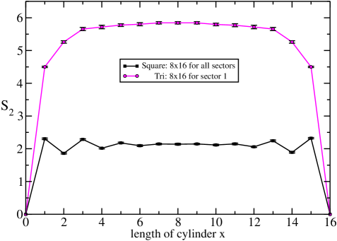
Figure 6: SQUARE-TRIANGULAR: $S_{2}$ for the RVB wave function on the square and triangular (Tri) lattice is shown. The RVB wave function is sampled over all topological sectors for the square lattice, whereas in the triangular case, we fix the topological sector. The different behavior of the EE $S_{2}$ reflects the critical and gapped nature of the RVB state on the respective lattice.

We point out that if we calculate the EE $S_{2}$ over a cylindrical area, using (18) is sufficient. However, for a Levin-Wen construction the re-weighting scheme must be used in order to obtain sufficiently small error bars. For all Levin-Wen calculations in the Letter, a step width of $r_{i+1}-r_{i}=0.2$ was used. Subsequently, the amplitude-dependent part of the SWAP-operator is a product (24) consisting of $5$ factors. Adding a single calculation for the sign-dependent part of SWAP, we find that each Levin-Wen region $A$ requires six different calculations, the product of six partial expectation values corresponds to the “full” expectation value $\langle\text{SWAP}\rangle$.

In the case of the RVB states on the triangular and kagome lattice, we remark that the error bars of all expectation values of the amplitude-part of the SWAP-operator converge relatively fast and are of order $10^{-4(5)}$. However, the error stemming from the sign-part $\langle\text{SWAP}_{sign}\rangle$ is significantly larger with values of $~{}0.2$ and $~{}0.3$ for the two lattices.

As an example for an entanglement calculation without re-weighting scheme, we show the EE $S_{2}$ for a $12\times 12$-square lattice for cylindrical regions in Fig. 5. For bipartite lattices such as the square lattice, it is generally possible to sample over valence bond configurations, or perform a “loop gas” mapping Sutherland (1988), without encountering a sign problem. Here, Marshall’s sign rule provides a unique way of orientating all links, so that all statistical weights, which are given by valence bond state overlaps, are positive. For the bipartite square lattice, instead of four topological sectors, one has an extensive number of sectors. When using Valence Bond Monte Carlo (VBMC), it is possible to sample within a fixed sector, since here we start from a certain valence bond configuration and only perform local updates that can never lead into another sector.

Contrarily, the Pfaffian MC cannot project onto a single sector on the square lattice, instead we sum over all topological sectors. However, we find that the behavior of the entanglement entropy $S_{2}$ does not depend on a specific sector or even the sum over all sectors (see Fig. 5).

3) Comparison between the EE $S_{2}$ for the triangular and the square lattice and finite size effects. –

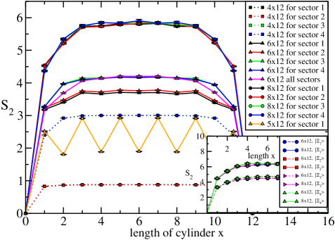
Figure 7: TRIANGULAR: A comparison for $S_{2}$ for cylindrical regions between sectors $1,2,3$ and $4$ is shown. We observe that for large enough system size, the EE $S_{2}$ is the same for all four sectors. The inset shows $S_{2}$ for cylindrical regions for all four MES-states $|\Xi_{i}\rangle$, $i=1,\ldots,4$. It is evident that the four states $|\Xi_{i}\rangle$ become indistinguishable by their EE $S_{2}$ within errors for sufficiently large system sizes.

We do a comparison of the EE $S_{2}$ for cylindrical regions $A$, via Pfaffian Monte Carlo on square and triangular lattices of the same size ($M\times 2N=8\times 16$). As discussed in the previous Section $2)$, the Pfaffian MC cannot project onto a single topological sector in the case of the square lattice. Hence, we sum over all sectors for the square lattice, and fix the topological sector for the triangular case. Fig. 6 shows fundamentally different behavior in the EE $S_{2}$ for these two lattices. For the square lattice, we observe an “even/odd” or zig-zag effect that was investigated previously in Refs.Ju et al. (2012) and Stéphan et al. (2013). Fig. 6 shows a weak oscillating behavior for growing cylinder length, which becomes much more pronounced in larger system sizes, and lattices that have a $M/2N$-ratio higher than $1/2$ Ju et al. (2012); Stéphan et al. (2013). The specific shape dependence of the even and odd branches is a reflection of the critical theory related to the square-lattice RVB wave function, which is conjectured to be related to a $2D$ quantum Lifshitz critical point Stéphan et al. (2013).

In contrast, $S_{2}$ obtained from the triangular lattice does not display critical behavior, including the absence of the even/odd effect.

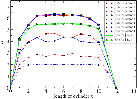
Figure 8: KAGOME: A comparison of $S_{2}$ for cylindrical regions between sectors $1,2,3$ and $4$ on the kagome lattice. We observe that for large enough system sizes $(M,N)=(3,4)$ amounting to $72$ lattice sites, the EE $S_{2}$ is the same for all four sectors within error bars. Further, we present the EE $S_{2}$ for the MES-states by showing two examples corresponding to $|\Xi_{1}\rangle$ and $|\Xi_{3}\rangle$ for $(M,N)=(3,4)$. The other two MES-states not shown here, $|\Xi_{2,4}\rangle$, exhibit the analogous behavior. Since $S_{2}$ is the same for all topological sectors, we expect and confirm that $S_{2}$ is the same for all MES-states within errors according to the MES-states ansatz in Eq.(3) in the Letter.

Rather, $S_{2}$ saturates quickly away from cylinder lengths $x=0$ and $x=2N$, becoming independent of the system size $A$ (to within error bars). This “flat” behavior in the EE $S_{2}$ reflects the fact that the triangular lattice RVB wave function is the ground state of a gapped local Hamiltonian, in contrast with the square lattice case which is critical.

Fig. 7 shows more data on the triangular lattice. Shown is $S_{2}$ obtained for all four wave functions $|\Psi_{i}\rangle$, $i=1,\ldots,4$, and for the equal amplitude superposition of all four wave functions, $|\Psi_{\text{all sec}}\rangle=\sum_{i=1}^{4}|\Psi_{i}\rangle$, for lattices of sizes $M\times 2N=4,5,6,8\times 12$.

We note that we see a certain “even/odd” effect in $x$ for odd $M=5$. This can be shown to be a finite size effect present for odd $M$ when $M\ll 2N$. It stems from the fact that for odd cylinder length $x$, there are less dimerizations corresponding to the Ising state that the sysem is in than there are for even length $x$. Thus, the values of $S_{2}$ at odd $x$ are larger than the ones at even $x$. The “up/down”-pattern becomes less pronounced when we increase odd $M$ and finally vanishes. We stress that still the $S_{2}$ for odd (even) $x$ saturates and does not depend on odd (even) $x$ once a minimal size of region $A$ is reached.

Furthermore, we notice differences in the respective $S_{2}$ belonging to a certain sector for sizes $4,6\times 12$. Again, this is a finite size effect, and for a large enough system, e.g. $8\times 12$, we do not observe differences in $S_{2}$ within error bars for different sectors.

We also note that the equal amplitude superposition of all four sectors, $|\Psi_{\text{all sec}}\rangle$, should deliver the same EE $S_{2}$ as a single sector. The reason for that is that all states $|\Psi_{i}\rangle$, $i=1,\ldots,4$, and $|\Psi_{\text{all sec}}\rangle$ have the same TEE $-\gamma^{\prime}$ (see Section 4$)$).

In Fig. 7, we observe that for a system of size $6\times 12$, sectors $3$ and $4$ have the same EE $S_{2}$ within error bars as $|\Psi_{\text{all sec}}\rangle$. We conclude that in this case only the other two sectors, $1$ and $2$, suffer from finite size effects.

The same effects can be found in the kagome lattice in Fig. $3$ in the Letter and in Fig. 8. Fig. 8 shows that for the kagome lattice, we need a system size of $(M,N)=(3,4)$, amounting to $72$ sites, in order to achieve equality within error bars for the EE $S_{2}$ for all four sectors. Further, Fig. 8 shows that for $N\leq 4$ with fixed $M=3$, we still see differences between the single sectors, including a zig-zag effect similar to the triangular lattice. Again, as in the triangular case, we see that $S_{2}$ also quickly experiences saturation once a minimum cylinder length $x$ is reached which strongly indicates that the Hamiltonian derived in Ref.Seidel (2009), which has the RVB state as its unique groundstate modulo topological degeneracy, is gapped.

4) Ground-state dependence of the TEE $-\gamma$. – The TEE $-\gamma$ is independent of the state used to calculate the Renyi entropy $S_{n}$ as long as the region $A$ is contractible. In the case that the area $A$ has at least one non-contractible boundary such as a cylindrical cut, $\gamma$ becomes state-dependent. If we now express any state in the basis of the so-called minimum entropy states (MES-states) Zhang et al. (2012), $|\Psi_{\alpha}\rangle=\sum_{j}c_{j}|\Xi_{j}\rangle$, and take the area $A$ to be a torus with two non-contractible boundaries, then we have

$$\gamma_{n}^{\prime}(\{p_{j}\})=2\gamma+\frac{1}{n-1}\text{ln}\bigg{(}\sum_{j}p_{j}^{n}d_{j}^{2(1-n)}\bigg{)}\;.$$ (25)

In the expression above, the sum over $j$ runs over all quasiparticles of the theory. The states $|\Xi_{j}\rangle$, $j=1,\ldots,4$, can be obtained by inserting a quasiparticle into the system. The $d_{j}\geq 1$ are the quantum dimensions of each quasiparticle and the $p_{j}$ in (25) are $p_{j}=|c_{j}|^{2}$.

As stated previously, in this Letter we focus on the second Renyi entropy and set $n=2$. Consequently, (25) simplifies to

$$\gamma^{\prime}(\{p_{j}\})=2\gamma+\text{ln}\bigg{(}\sum_{j}\frac{p_{j}^{2}}{d_{j}^{2}}\bigg{)}\;.$$ (26)

The numerical data shows the entanglement entropy to be independent of the wave functions $|\Psi_{i}\rangle$ used to calculate it for large enough systems for the kagome and the triangular lattice. Consequently, $\gamma^{\prime}$ has to be the same for all four states $|\Psi_{i}\rangle$, $i=1,\ldots,4$. We determined the value of $\gamma^{\prime}$ for both the triangular and the kagome to be close to $\text{ln}(2)$ if a single topological sector $|\Psi_{i}\rangle$, $i=1,\ldots,4$, is used to calculate it. In the Letter, we argued that the underlying quantum field theory must be an Abelian theory. Thus, all quasiparticles have the same quantum dimension $d=1$. This implies that each wave function $|\Psi_{i}\rangle$ is a superposition of two MES-states:

$$|\Psi_{i}\rangle=\frac{1}{\sqrt{2}}\big{(}|\Xi_{a}\rangle\pm|\Xi_{b}\rangle\big{)}\;,$$ (27)

with $(a,b)=(1,2),(3,4)$. For later purposes, we also give $\gamma^{\prime}$ belonging to a single MES-state $|\Xi_{i}\rangle$, $i=1,\ldots,4$:

$$|\Psi_{i}\rangle:\;\;\;\;\gamma^{\prime} = 2\;\text{ln}(2)+\text{ln}\bigg{(}\frac{1}{4}+\frac{1}{4}\bigg{)}=\text{ln}(2)\approx 0.69$$

$$|\Xi_{i}\rangle:\;\;\;\;\gamma^{\prime} = 2\;\text{ln}(2)+\text{ln}\big{(}1\big{)}=2\;\text{ln}(2)\approx 1.38\;.$$

5) MES-states for a dimer model on the triangular/kagome lattice. – The short-ranged dimer model on the kagome and the triangular lattice is known to be a $\mathbb{Z}_{2}$ liquid with toric code anyonic excitations. We will now derive the MES-states for this system. Note that we closely follow a similar derivation for the toric code model Zhang et al. (2012).

We recall that the $\mathbb{Z}_{2}$ dimer model has four topological sectors that are distinguished by the number of dimer cuts of a loop along each of the two directions of the lattice. For convenience, we temporarily use the subscripts ’$0$’ for an even of dimer cuts and ’$1$’ for an odd number, instead of ’$e$’ and ’$o$’, respectively. We only distinguish between even ($0$) and odd ($1$) number of cuts, thus, the four sectors are labeled: $(ab)=(00),(01),(10)$, and $(11)$. We denote a single sector by

$$|\Psi_{ab}\rangle=\sum_{D\in(ab)}|D\rangle\;.$$ (29)

Thus, in general, we can write a superposition of all four sectors as:

$$|\Psi\rangle=\sum_{(ab)}c_{ab}|\Psi_{ab}\rangle\;.$$ (30)

We proceed by doing a Schmidt decomposition of the states (29). For this sake, we define a virtual cut $\Delta$ along the $\vec{a}$-direction (see Fig. $1$ in Letter) and define $|\Psi_{\{q_{l}\}b}^{A(B)}\rangle$ as the normalized equal superposition of all possible dimer coverings in subsystem $A(B)$. The boundaries defining the subsystems $A,B$ are along the $\vec{b}$-direction.

The boundary condition connecting the two subsystems $A$ and $B$ is specified by $\{q_{l}=0,1\}$, $l=1,2,\ldots,L$ ($L$ = total length of boundaries) and the number of dimer crossings of the virtual cut $\Delta$ modulo $2$ equals $b=0,1$. Consequently, the Schmidt-decomposed state is

$$|\Psi_{ab}\rangle = \frac{1}{\sqrt{2N_{q}}}\sum_{\{q_{l}\}\in a}\bigg{(}|\Psi_{\{q_{l}\}0}^{A}\rangle|\Psi_{\{q_{l}\}b}^{B}\rangle$$

$$\hskip 56.9055pt+|\Psi_{\{q_{l}\}1}^{A}\rangle|\Psi_{\{q_{l}\}b+1}^{B}\rangle\bigg{)}\;.$$

In the above, $\{q_{l}\in a=0(1)\}$ denotes that only an even (odd) number of dimer crossings is allowed at the boundary $L_{1}$. The second boundary $L_{2}$ must have the same type, even or odd, of dimer cuts. The total length $L$ of the boundary is the combined length of $L_{1}$ and $L_{2}$. Subsequently, the total number of valid boundary conditions $\{q_{l}\}\in a$ in each parity sector is $N_{q}=2^{L-2}$. We now replace all four terms in (30) with the corresponding Schmidt-decomposed state, form the outer product $|\Psi\rangle\langle\Psi|$ and execute the trace over the subspace $B$. This will give the reduced density matrix $\rho_{A}$:

$$\rho_{A} = \frac{1}{\sqrt{2N_{q}}}\sum_{\{q_{l}\;even\}}\bigg{[}(|c_{00}|^{2}+|c_{01}|^{2})\bigg{(}|\Psi_{\{q_{l}\}0}^{A}\rangle\langle\Psi_{\{q_{l}\}0}^{A}|$$ (32)

$$\hskip 136.5733pt+\;|\Psi_{\{q_{l}\}1}^{A}\rangle\langle\Psi_{\{q_{l}\}1}^{A}|\bigg{)}$$

$$+ 2\text{Real}(c_{00}^{\ast}c_{01})\bigg{(}|\Psi_{\{q_{l}\}0}^{A}\rangle\langle\Psi_{\{q_{l}\}1}^{A}|+|\Psi_{\{q_{l}\}1}^{A}\rangle\langle\Psi_{\{q_{l}\}0}^{A}|\bigg{)}\bigg{]}$$

$$+ \frac{1}{\sqrt{2N_{q}}}\sum_{\{q_{l}\;odd\}}\bigg{[}(|c_{10}|^{2}+|c_{11}|^{2})\bigg{(}|\Psi_{\{q_{l}\}0}^{A}\rangle\langle\Psi_{\{q_{l}\}0}^{A}|$$

$$\hskip 136.5733pt+\;|\Psi_{\{q_{l}\}1}^{A}\rangle\langle\Psi_{\{q_{l}\}1}^{A}|\bigg{)}$$

$$+ 2\text{Real}(c_{10}^{\ast}c_{11})\bigg{(}|\Psi_{\{q_{l}\}0}^{A}\rangle\langle\Psi_{\{q_{l}\}1}^{A}|+|\Psi_{\{q_{l}\}1}^{A}\rangle\langle\Psi_{\{q_{l}\}0}^{A}|\bigg{)}\bigg{]}$$

$$= \frac{1}{2N_{q}}\sum_{\{q_{l}\;even\}}\bigg{[}|c_{00}+c_{01}|^{2}|\Psi_{\{q_{l}\}+}^{A}\rangle\langle\Psi_{\{q_{l}\}+}^{A}|$$

$$\hskip 54.06006pt+|c_{00}-c_{01}|^{2}|\Psi_{\{q_{l}\}-}^{A}\rangle\langle\Psi_{\{q_{l}\}-}^{A}|\bigg{]}$$

$$+ \frac{1}{2N_{q}}\sum_{\{q_{l}\;odd\}}\bigg{[}|c_{10}+c_{11}|^{2}|\Psi_{\{q_{l}\}+}^{A}\rangle\langle\Psi_{\{q_{l}\}+}^{A}|$$

$$\hskip 54.06006pt+|c_{10}-c_{11}|^{2}|\Psi_{\{q_{l}\}-}^{A}\rangle\langle\Psi_{\{q_{l}\}-}^{A}|\bigg{]}$$

with

$$|\Psi_{\{q_{l}\}\pm}^{A}\rangle=\frac{1}{\sqrt{2}}(|\Psi_{\{q_{l}\}0}^{A}\rangle\pm|\Psi_{\{q_{l}\}1}^{A}\rangle).$$ (33)

The two states (33) are orthogonal to each other, as are the different dimer states that were summed over when the trace was taken in order to obtain $\rho_{A}$.

Armed with this, we now calculate the $n$-th Renyi entropy $S_{n}$:

$$S_{n} = \frac{1}{1-n}\text{ln}(\text{Tr}\rho_{A}^{n})$$ (34)

$$= \frac{1}{n-1}\text{ln}\bigg{[}\bigg{(}\frac{1}{2N_{q}}\bigg{)}^{2}N_{q}\bigg{(}(|c_{00}+c_{01}|^{2})^{n}$$

$$\hskip 91.04872pt+(|c_{00}-c_{01}|^{2})^{n}$$

$$\hskip 91.04872pt+(|c_{10}+c_{11}|^{2})^{n}$$

$$\hskip 91.04872pt+(|c_{10}-c_{11}|^{2})^{n}\bigg{)}\bigg{]}$$

$$= \text{ln}(N_{q})+\frac{1}{1-n}\text{ln}\bigg{(}\sum_{j=1}^{4}p_{j}^{n}\bigg{)}$$

$$= L\text{ln}(2)-\bigg{[}2\text{ln}(2)+\frac{1}{n-1}\text{ln}\bigg{(}\sum_{j}p_{j}^{n}\bigg{)}\bigg{]}$$

with

$$p_{1}=\frac{|c_{00}+c_{01}|^{2}}{2}\;\;\;\;\;\;\;\;\;p_{2}=\frac{|c_{00}-c_{01}|^{2}}{2}$$

$$p_{3}=\frac{|c_{10}+c_{11}|^{2}}{2}\;\;\;\;\;\;\;\;\;p_{4}=\frac{|c_{10}-c_{11}|^{2}}{2}\;.$$ (35)

Thus, up to an overall phase $e^{i\Phi_{j}}$, $j=1,\ldots,4$, the MES-states (that are orthogonal to each other) along $\vec{b}$ are each a superposition of two specific topological sectors:

$$|\Xi_{1}\rangle=\frac{e^{i\Phi_{1}}}{\sqrt{2}}(|\Psi_{ee}\rangle+|\Psi_{eo}\rangle)\;,$$

$$|\Xi_{2}\rangle=\frac{e^{i\Phi_{2}}}{\sqrt{2}}(|\Psi_{ee}\rangle-|\Psi_{eo}\rangle)\;,$$

$$|\Xi_{3}\rangle=\frac{e^{i\Phi_{3}}}{\sqrt{2}}(|\Psi_{oo}\rangle+|\Psi_{oe}\rangle)\;,$$

$$|\Xi_{4}\rangle=\frac{e^{i\Phi_{4}}}{\sqrt{2}}(|\Psi_{oo}\rangle-|\Psi_{oe}\rangle)\;.$$ (36)

We note that the analogous MES-states were previously found in Ref.Zhang et al. (2012) for the toric code model. In the case of the toric code, $|\Psi_{\{q_{l}\}b}^{A(B)}\rangle$ is defined to be the normalized equal superposition of all possible configurations of closed-loop strings $C$ in subsystem $A(B)$. Obviously, the degrees of freedom for the toric code model are the closed-loop strings $C$. For a dimer model, the above derivation of the MES-states is extremely similar to the toric code calculation once the degrees of freedom, the closed-loop strings, have been replaced by dimer degrees of freedom.

There is an obvious correspondence between certain topological sectors of exactly solvable $\mathbb{Z}_{2}$ model systems, such as the toric code, the dimer model on the kagome and the triangular lattices, etc. $\ldots$, leading to a generic relation between these sectors and the MES-states, described by a matrix $T$ (see Section $6)$). To clarify this issue and especially to make clear that MES-states for double semion statistics have to be different, we will now investigate the transformation behavior of MES-states under modular transformations.

6) Modular $\mathcal{U}$- and $\mathcal{S}$-matrices and MES-states for the RVB spin liquid on the triangular/kagome lattice. – We will now determine the $\mathcal{U}$- and $\mathcal{S}$-matrices describing the quasiparticle statistics of the RVB system on the kagome and the triangular lattice by using the transformation behavior of the four (numerically confirmed) MES-states $|\Xi_{i}\rangle$, $i=1,\ldots,4$, under a certain modular transformation of the primitive lattice vectors $\vec{a}$ and $\vec{b}$.

To start, we state that the $\mathcal{S}$- and $\mathcal{U}$-matrices describe the action of modular transformations on the degenerate ground-state manifold of the underlying topological quantum field theory on a torus. These two transformations generate the so-called modular group $SL(2,\mathbb{Z})$. All elements of this group can be generated by successive application of the following two generators $\mathfrak{s}$ and $\mathfrak{u}$, represented by the following matrix action on lattice vectors $\vec{a},\vec{b}$: $S=\begin{pmatrix}\;\;\;0&1\cr-1&0\cr\end{pmatrix}$ and $U=\begin{pmatrix}1&1\cr 0&1\cr\end{pmatrix}$.

Here, we refer the reader for more details to Ref.Zhang et al. (2012) and proceed by transforming the two primitive vectors $\vec{a}$ and $\vec{b}$ by applying $\mathfrak{us}^{-1}$ to them. This transformation, referred to as $R_{\pi/3}$ in the following, corresponds to: $\vec{a}\rightarrow\vec{a}-\vec{b}$ and $\vec{b}\rightarrow\vec{a}$. In this section, we consider kagome lattices of dimensions $(M,N)=(M,2M)$ and triangular lattices of size $(M,2N)=(2N,2N)$. For this choice of $(M,N)$ and $(M,2N)$ for the respective lattice, we have as many links in $\vec{a}$-direction as in $\vec{b}$-direction and transforming the primitive vectors as described above corresponds to a rotation of the system by $\pi/3$. Hence, the name $R_{\pi/3}$.

According to Ref.Zhang et al. (2012), the overlaps $V_{ij}=\langle\Xi_{i}|R_{\pi/3}|\Xi_{j}\rangle$ between the bases $\{|\Xi_{i}\rangle\}$ and $\{R_{\pi/3}|\Xi_{j}\rangle\}$ form the unitary transformation $V=D^{\dagger}US^{-1}D$, where $D$ is a diagonal matrix of phases $D_{jj}=e^{i\Phi_{j}}$ corresponding to the phase freedom of choosing $|\Xi_{j}\rangle$.

We now explicitly construct the $\mathcal{US}^{-1}$-matrices for toric code and for double semion quasiparticle statistics. The $\mathcal{U}$-matrix is a diagonal matrix with its $ii$th entry corresponding to the phase the $i$th quasiparticle acquires when it is exchanged with an identical one. Note that for the toric code anyon model, the quasiparticles consist of three bosons and one fermion. Thus, the self statistics yield phases of $1$ (bosons) and $-1$ (fermion). Contrarily, the double semion anyon model consists of two bosons, one semion and one anti-semion. In this case, the self statistics yield phases of $1$ (bosons), $i$ (semion) and $-i$ (anti-semion).

For Abelian phases, the $ij$th entry of the $\mathcal{S}$-matrix corresponds to the phase the $i$th quasiparticle acquires when it encircles the $j$th quasiparticle.

For the toric code, we have

$$\mathcal{U}=\begin{pmatrix}1&0&0&\;\;\;0\\ 0&1&0&\;\;\;0\\ 0&0&1&\;\;\;0\\ 0&0&0&-1\end{pmatrix},\quad\mathcal{S}=\frac{1}{2}\begin{pmatrix}1&\;\;\;1&\;\;\;1&\;\;\;1\\ 1&\;\;\;1&-1&-1\\ 1&-1&\;\;\;1&-1\\ 1&-1&-1&\;\;\;1\end{pmatrix},$$ (37)

while for the double semion phase, we have

$$\mathcal{U}=\begin{pmatrix}1&0&0&\;\;\;0\\ 0&1&0&\;\;\;0\\ 0&0&i&\;\;\;0\\ 0&0&0&-i\end{pmatrix},\quad\mathcal{S}=\frac{1}{2}\begin{pmatrix}1&\;\;\;1&\;\;\;1&\;\;\;1\\ 1&\;\;\;1&-1&-1\\ 1&-1&-1&\;\;\;1\\ 1&-1&\;\;\;1&-1\end{pmatrix}.$$ (38)

We now construct the $\mathcal{US}^{-1}$-matrices. In the case of toric code statistics, we have

$$\mathcal{US}^{-1}=\frac{1}{2}\begin{pmatrix}\;\;\;1&\;\;\;1&\;\;\;1&\;\;\;1\\ \;\;\;1&\;\;\;1&-1&-1\\ \;\;\;1&-1&\;\;\;1&-1\\ -1&\;\;\;1&\;\;\;1&-1\end{pmatrix}.$$ (39)

In the case of double semion statistics, the $\mathcal{US}^{-1}$-matrix is given by

$$\mathcal{US}^{-1}=\frac{1}{2}\begin{pmatrix}\;\;\;1&\;\;\;1&\;\;\;1&\;\;\;1\\ \;\;\;1&\;\;\;1&-1&-1\\ \;\;\;i&-i&-i&\;\;\;i\\ -i&\;\;\;i&-i&\;\;\;i\end{pmatrix}.$$ (40)

The crucial difference lies therein that the $\mathcal{US}^{-1}$-matrix for the toric code quasiparticle statistics is a real matrix, contrarily the $\mathcal{US}^{-1}$-matrix for double semion statistics has real and complex entries. Thus, we conclude that $D$, the diagonal matrix of phases $D_{jj}=e^{i\Phi_{j}}$ corresponding to the phase freedom of choosing $|\Xi_{j}\rangle$, can be choosen to be real in the case of toric code statistics. This leads to a real matrix $V_{ij}$ in the basis of the MES-states.

However, for double semion quasiparticle statistics, there exists no such choice of phases $D_{jj}$ that renders all overlap matrix elements $V_{ij}$ real in the MES-states basis. Thus, we showed that the MES-states (Entanglement Entropy and Topological Order in Resonating Valence-Bond Quantum Spin Liquids) are uniquely connected/bound to toric code statistics.

To close this section, we derive the behavior of the four states $|\Psi_{\alpha\beta}\rangle$, $(\alpha\beta)=(ee),(eo),(oe),(oo)$ under $\pi/3$-rotation and then construct the matrix $T(T^{\dagger})$ which governs the change of basis from $|\Psi_{\alpha\beta}\rangle$-states to $|\Xi_{i}\rangle$-states (and vice versa). We recall that the lattices in this section are of sizes $(M,N)=(M,2M)$ for the kagome and $(M,2N)=(2N,2N)$ for the triangular lattice, and now distinguish between an even and odd choice of $M$ for the kagome, and, respectively, between an even and odd choice of $N$ for the triangular lattice Poilblanc and Misguich (2011). We observe that if we choose $M(N)$ to be even for the kagome (triangular) lattice, the four topological sectors transform as

$$R_{\pi/3}|\Psi_{ee}\rangle=|\Psi_{ee}\rangle\,,\;\; R_{\pi/3}|\Psi_{eo}\rangle=|\Psi_{oe}\rangle$$

$$R_{\pi/3}|\Psi_{oe}\rangle=|\Psi_{oo}\rangle\,,\;\; R_{\pi/3}|\Psi_{oo}\rangle=|\Psi_{eo}\rangle\;.$$ (41)

We now assume all phases $e^{i\Phi_{j}}$ in (Entanglement Entropy and Topological Order in Resonating Valence-Bond Quantum Spin Liquids) to be one. This will give the following basis transformation matrix $T$:

$$T=\frac{1}{\sqrt{2}}\begin{pmatrix}1&\;\;\;1&\;\;\;0&\;\;\;0\\ 1&-1&\;\;\;0&\;\;\;0\\ 0&\;\;\;0&\;\;\;1&\;\;\;1\\ 0&\;\;\;0&\;\;\;1&-1\end{pmatrix}.$$ (42)

We note that $T^{\dagger}=T$ and proceed by constructing $T^{\dagger}R_{\pi/3}T$:

$$T^{\dagger}R_{\pi/3}T=$$

$$\frac{1}{\sqrt{2}}\begin{pmatrix}1&\;\;\;1&0&\;\;\;0\\ 1&-1&0&\;\;\;0\\ 0&\;\;\;0&1&\;\;\;1\\ 0&\;\;\;0&1&-1\end{pmatrix}\begin{pmatrix}1&0&0&0\\ 0&0&1&0\\ 0&0&0&1\\ 0&1&0&0\end{pmatrix}\frac{1}{\sqrt{2}}\begin{pmatrix}1&\;\;\;1&0&\;\;\;0\\ 1&-1&0&\;\;\;0\\ 0&\;\;\;0&1&\;\;\;1\\ 0&\;\;\;0&1&-1\end{pmatrix}$$

$$=\frac{1}{2}\begin{pmatrix}\;\;\;1&\;\;\;1&\;\;\;1&\;\;\;1\\ \;\;\;1&\;\;\;1&-1&-1\\ \;\;\;1&-1&\;\;\;1&-1\\ -1&\;\;\;1&\;\;\;1&-1\end{pmatrix}.$$ (43)

The matrix (43) is indeed the same as matrix (39). Thus, our choice of phases $D_{jj}=e^{i\Phi_{j}}=1$ for all four MES-states $|\Xi_{j}\rangle$, $j=1,\ldots,4$, listed in (Entanglement Entropy and Topological Order in Resonating Valence-Bond Quantum Spin Liquids) reproduces the $\mathcal{US}^{-1}$-matrix for toric code quasiparticle statistics (39).

Subsequently, we give the transformation behavior of the four topological sectors for odd $M(N)$ for the kagome (triangular) lattice:

$$R_{\pi/3}|\Psi_{ee}\rangle=|\Psi_{oe}\rangle\,,\;\; R_{\pi/3}|\Psi_{eo}\rangle=|\Psi_{ee}\rangle$$

$$R_{\pi/3}|\Psi_{oe}\rangle=|\Psi_{eo}\rangle\,,\;\; R_{\pi/3}|\Psi_{oo}\rangle=|\Psi_{oo}\rangle\;.$$ (44)

One can now repeat the contruction of $T^{\dagger}R_{\pi/3}T$ in order to obtain the $\mathcal{US}^{-1}$-matrix in MES-basis again. In the case of odd $M(N)$ for the kagome (triangular) lattice, one can show that the appropriate phases, $D_{jj}=e^{i\Phi_{j}}$, are $D_{jj}=\{1,-1,1,-1\}$ for the MES-states $|\Xi_{j}\rangle$, $j=1,\ldots,4$, in (Entanglement Entropy and Topological Order in Resonating Valence-Bond Quantum Spin Liquids).

To summarize, these considerations show that our numerically confirmed MES-states for the kagome and triangular systems indeed imply the statistics of the $\mathbb{Z}$ phase, ruling out in particular double semion statistics. Thus, we have unambiguously identified the underlying quasiparticle statistics to be toric code statistics, taking into account that we already identified the topological entanglement entropy (TEE) $-\gamma$ to be $-\gamma=-\text{ln}(2)$ as expected for a topological $\mathbb{Z}_{2}$ spin liquid.

After identifying the MES-states for the RVB state on the kagome and the triangular lattice, we note that all wave functions $|\Psi_{\alpha\beta}\rangle$, $(\alpha\beta)=(ee),(eo),(oe),(oo)$, are superpositions of the form

$$|\Psi_{\alpha\beta}\rangle=\frac{1}{\sqrt{2}}\big{(}|\Xi_{a}\rangle\pm|\Xi_{b}\rangle\big{)}\;,$$ (45)

with $(a,b)=(1,2),(3,4)$.

The numerical data shows the entanglement entropy $S_{2}$ to be independent of the sector and to be independent of the MES-state $|\Xi_{i}\rangle$, $i=1,\ldots,4$, used to calculate it, respectively. Again, this implies that $\gamma^{\prime}$ is the same for all $|\Psi_{\alpha\beta}\rangle$, $(\alpha,\beta)=(ee),(eo),(oe),(oo)$, and for all $|\Xi_{i}\rangle$, $i=1,\ldots,4$, respectively. A direct consequence of the latter is that all four quasiparticles belonging to the four MES-states must have the same quantum dimension $d_{i}$. Since every phase, Abelian and non-Abelian, has (at least) one quasiparticle with quantum dimension $d=1$, we conclude that all quasiparticles have $d_{i}=1$, $i=1,\ldots,4$. While this does not identify the topological phase, it again numerically confirms that the phase has to be Abelian.

For reasons of completeness, we now give the other set of MES-states $\{|\Xi_{i}^{\prime}\rangle\}$ obtained for cuts along $\vec{a}$. For cuts along the other direction, $\vec{a}$, we obtain the corresponding MES-states from the action of the modular $\mathcal{S}$-matrix on the MES-states for cuts along the $\vec{b}$-direction:

$$|\Xi_{1}\rangle\longrightarrow\frac{1}{2}(|\Xi_{1}\rangle+|\Xi_{2}\rangle+|\Xi_{3}\rangle+|\Xi_{4}\rangle)\;,$$

$$|\Xi_{2}\rangle\longrightarrow\frac{1}{2}(|\Xi_{1}\rangle+|\Xi_{2}\rangle-|\Xi_{3}\rangle-|\Xi_{4}\rangle)\;,$$

$$|\Xi_{3}\rangle\longrightarrow\frac{1}{2}(|\Xi_{1}\rangle-|\Xi_{2}\rangle+|\Xi_{3}\rangle-|\Xi_{4}\rangle)\;,$$

$$|\Xi_{4}\rangle\longrightarrow\frac{1}{2}(|\Xi_{1}\rangle-|\Xi_{2}\rangle-|\Xi_{3}\rangle+|\Xi_{4}\rangle)\;.$$ (46)

leading to

$$|\Xi_{1}^{\prime}\rangle=\frac{1}{\sqrt{2}}(|\Psi_{oo}\rangle+|\Psi_{ee}\rangle)\;,$$

$$|\Xi_{2}^{\prime}\rangle=\frac{1}{\sqrt{2}}(|\Psi_{oo}\rangle-|\Psi_{ee}\rangle)\;,$$

$$|\Xi_{3}^{\prime}\rangle=\frac{1}{\sqrt{2}}(|\Psi_{eo}\rangle+|\Psi_{oe}\rangle)\;,$$

$$|\Xi_{4}^{\prime}\rangle=\frac{1}{\sqrt{2}}(|\Psi_{eo}\rangle-|\Psi_{oe}\rangle)\;.$$ (47)

Here, we fixed the phases in (Entanglement Entropy and Topological Order in Resonating Valence-Bond Quantum Spin Liquids) as seen/explained in Ref.Zhang et al. (2012).

In order to extract the TEE $-\gamma^{\prime}$ from cylindrical bipartitions of the respective lattice, we checked the behavior of the EE $S_{2}$ for the MES-states and the respective so-called nonMES-states. A nonMES-states is any linear combination of more than one MES-state. Here, we restrict ourselves to nonMES-states, referred to as $|\Sigma_{i}\rangle$ in the following, which are certain superpositions of exactly two topological sectors that are not leading to a single MES-state from (Entanglement Entropy and Topological Order in Resonating Valence-Bond Quantum Spin Liquids), e.g.

$$|\Sigma_{1}^{\prime}\rangle=\frac{1}{\sqrt{2}}(|\Psi_{ee}\rangle+|\Psi_{\alpha}\rangle)\;,$$

$$|\Sigma_{2}^{\prime}\rangle=\frac{1}{\sqrt{2}}(|\Psi_{ee}\rangle-|\Psi_{\alpha}\rangle)\;,$$

$$|\Sigma_{3}^{\prime}\rangle=\frac{1}{\sqrt{2}}(|\Psi_{eo}\rangle+|\Psi_{\beta}\rangle)\;,$$

$$|\Sigma_{4}^{\prime}\rangle=\frac{1}{\sqrt{2}}(|\Psi_{eo}\rangle-|\Psi_{\beta}\rangle)\;.$$ (48)

with $\alpha=(eo),(oe)$ and $\beta=(oo),(ee)$. One can easily show that they are equal weight superpositions of all four MES-states (Entanglement Entropy and Topological Order in Resonating Valence-Bond Quantum Spin Liquids). The state-dependent TEE vanishes in this case: $\gamma^{\prime}=0$.

The corresponding plots are shown in Fig. $3$ in the Letter, $S_{2}$ is the same for the two nonMES-states and it is larger than $S_{2}$ for the respective MES-state. Since we previously pointed out that $\gamma^{\prime}$ reaches its maximum $2\gamma$ (and $S_{2}$ its minimum) when calculating it with a MES-state, we can conclude that the difference for sufficiently long cylinder lengths $x$ between the MES-state and the nonMES-states of type (Entanglement Entropy and Topological Order in Resonating Valence-Bond Quantum Spin Liquids) is also $2\gamma$. This is confirmed by Fig. $3$ in the Letter.

References

- Wen (1990) X. G. Wen, Int. J. Mod. Phys. B4, 239 (1990).
- Wen (2013) X.-G. Wen, ISRN Condensed Matter Physics 2013, 198710 (2013).
- Balents (2010) L. Balents, Nature 464, 199 (2010).
- Kaul et al. (2013) R. K. Kaul, R. G. Melko, and A. W. Sandvik, Annual Review of Condensed Matter Physics 4, 179 (2013).
- Levin and Wen (2006) M. Levin and X.-G. Wen, Physical Review Letters 96, 110405 (2006).
- Kitaev and Preskill (2006) A. Kitaev and J. Preskill, Phys. Rev. Lett. 96, 110404 (2006).
- Isakov et al. (2011) S. V. Isakov, M. B. Hastings, and R. G. Melko, Nature Physics 7, 772 (2011).
- Zhang et al. (2011) Y. Zhang, T. Grover, and A. Vishwanath, Physical Review B 84, 075128 (2011).
- Grover et al. (2013) T. Grover, Y. Zhang, and A. Vishwanath, New Journal of Physics 15, 025002 (2013).
- Zhu et al. (2014) W. Zhu, S. Gong, and D. Sheng, Journal of Statistical Mechanics: Theory and Experiment 2014, P08012 (2014).
- Zhang et al. (2012) Y. Zhang, T. Grover, A. Turner, M. Oshikawa, and A. Vishwanath, Physical Review B 85, 235151 (2012).
- Cincio and Vidal (2013) L. Cincio and G. Vidal, Physical Review Letters 110, 067208 (2013).
- Wildeboer and Seidel (2012) J. Wildeboer and A. Seidel, Physical Review Letters 109, 147208 (2012).
- Anderson (1973) P. W. Anderson, Mater. Res. Bull 8, 153 (1973).
- Seidel (2009) A. Seidel, Physical Review B 80, 165131 (2009).
- Schuch et al. (2010) N. Schuch, I. Cirac, and D. Pérez-García, Annals of Physics 325, 2153 (2010).
- Zhou et al. (2014) Z. Zhou, J. Wildeboer, and A. Seidel, Physical Review B 89, 035123 (2014).
- Eisert et al. (2010) J. Eisert, M. Cramer, and M. B. Plenio, Rev. Mod. Phys. 82, 277 (2010).
- Dong et al. (2008) S. Dong, E. Fradkin, R. G. Leigh, and S. Nowling, Journal of High Energy Physics 2008, 016 (2008).
- Sutherland (1988) B. Sutherland, Physical Review B 37, 3786 (1988).
- Liang et al. (1988) S. Liang, B. Doucot, and P. Anderson, Physical Review Letters 61, 365 (1988).
- Sandvik (2005) A. W. Sandvik, Phys. Rev. Lett. 95, 207203 (2005).
- Albuquerque and Alet (2010) A. F. Albuquerque and F. Alet, Physical Review B 82, 180408 (2010).
- Tang et al. (2011) Y. Tang, A. W. Sandvik, and C. L. Henley, Physical Review B 84, 174427 (2011).
- Ju et al. (2012) H. Ju, A. B. Kallin, P. Fendley, M. B. Hastings, and R. G. Melko, Physical Review B 85, 165121 (2012).
- Stéphan et al. (2013) J.-M. Stéphan, H. Ju, P. Fendley, and R. G. Melko, New Journal of Physics 15, 015004 (2013).
- Punk et al. (2015) M. Punk, A. Allais, and S. Sachdev, arXiv preprint arXiv:1501.00978 (2015).
- Verstraete et al. (2006) F. Verstraete, M. M. Wolf, D. Perez-Garcia, and J. I. Cirac, Phys. Rev. Lett. 96, 220601 (2006).
- Schuch et al. (2012) N. Schuch, D. Poilblanc, J. I. Cirac, and D. Pérez-García, Phys. Rev. B 86, 115108 (2012).
- Iqbal et al. (2014) M. Iqbal, D. Poilblanc, and N. Schuch, Phys. Rev. B 90, 115129 (2014).
- Becca et al. (2011) F. Becca, L. Capriotti, A. Parola, and S. Sorella, in Introduction to Frustrated Magnetism (Springer, 2011), pp. 379–406.
- Yang and Yao (2012) F. Yang and H. Yao, Phys. Rev. Lett. 109, 147209 (2012).
- Hastings et al. (2010) M. B. Hastings, I. González, A. B. Kallin, and R. G. Melko, Physical Review Letters 104, 157201 (2010).
- Kallin et al. (2011) A. B. Kallin, M. B. Hastings, R. G. Melko, and R. R. P. Singh, Phys. Rev. B 84, 165134 (2011).
- (35) See the Supplemental Material.
- Poilblanc and Misguich (2011) D. Poilblanc and G. Misguich, Physical Review B 84, 214401 (2011).
- Kaul (2015) R. K. Kaul, Phys. Rev. Lett. 115, 157202 (2015).
- Islam et al. (2015) R. Islam, R. Ma, P. M. Preiss, M. E. Tai, A. Lukin, M. Rispoli, and M. Greiner, arXiv preprint arXiv:1509.01160 (2015).
- Troyer et al. (1998) M. Troyer, B. Ammon, and E. Heeb, Parallel Object Oriented Monte Carlo Simulations (Springer, 1998).
- Albuquerque et al. (2007) A. Albuquerque, F. Alet, P. Corboz, P. Dayal, A. Feiguin, S. Fuchs, L. Gamper, E. Gull, S. Gürtler, A. Honecker, et al., Journal of Magnetism and Magnetic Materials 310, 1187 (2007).
- Kasteleyn (1963) P. Kasteleyn, J. Math. Phys.(NY) 4, 287 (1963).
- (42) Since there is a one-to-one correspondence between dimer coverings and singlet coverings, the dimer partition function is equivalent to the singlet (RVB) partition function.
- Wu and Wang (2008) F. Wu and F. Wang, Physica A: Statistical Mechanics and its Applications 387, 4148 (2008).
- Pei et al. (2014) J. Pei, S. Han, H. Liao, and T. Li, Journal of Physics. Condensed matter: Institute of Physics journal 26, 035601 (2014).