A Deep Search for Prompt Radio Emission from Thermonuclear Supernovae with the Very Large Array

Abstract

Searches for circumstellar material around Type Ia supernovae (SNe Ia) are one of the most powerful tests of the nature of SN Ia progenitors, and radio observations provide a particularly sensitive probe of this material. Here we report radio observations for SNe Ia and their lower-luminosity thermonuclear cousins. We present the largest, most sensitive, and spectroscopically diverse study of prompt ($\Delta t\lesssim 1$ yr) radio observations of 85 thermonuclear SNe, including 25 obtained by our team with the unprecedented depth of the Karl G. Jansky Very Large Array. With these observations, SN 2012cg joins SN 2011fe and SN 2014J as a SN Ia with remarkably deep radio limits and excellent temporal coverage (six epochs, spanning 5–216 days after explosion, yielding $\dot{M}/v_{w}\lesssim 5\times 10^{-9}~{}{{{\rm M}_{\odot}\ {\rm yr}^{-1}}\over{{\rm 100\ km\ s}^{-1}}}$, assuming $\epsilon_{B}=0.1$ and $\epsilon_{e}=0.1$).

All observations yield non-detections, placing strong constraints on the presence of circumstellar material. We present analytical models for the temporal and spectral evolution of prompt radio emission from thermonuclear SNe as expected from interaction with either wind-stratified or uniform density media. These models allow us to constrain the progenitor mass loss rates, with limits ranging from $\dot{M}\lesssim 10^{-9}-10^{-4}$ M_⊙ yr^-1, assuming a wind velocity $v_{w}=100$ km s^-1. We compare our radio constraints with measurements of Galactic symbiotic binaries to conclude that $\lesssim$10% of thermonuclear SNe have red giant companions.

1. Introduction

The nature of the progenitors of Type Ia supernovae (SNe Ia) and other thermonuclear SNe (SNe Iax, Ca-rich SNe; SN 2002es-like explosions; Perets et al. 2010; Ganeshalingam et al. 2012; Foley et al. 2013) remains an important gap in our understanding of astrophysics, with important implications for cosmology, stellar phenomenology, and chemical evolution. There is general agreement that thermonuclear SNe involve a white dwarf in a binary system, but it remains unknown if the white dwarf is destabilized by reaching the Chandrasekhar mass, or if significantly sub-Chandrasekhar white dwarfs can explode as thermonuclear SNe. In addition, the nature of the binary companion remains a puzzle: it could be a red (super)giant, a subgiant, a main sequence star, or another white dwarf (Iben & Tutukov, 1984; Webbink, 1984). A wealth of review articles summarize these outstanding mysteries; see Branch et al. (1995); Livio (2001); Howell (2011); Wang & Han (2012); Maoz et al. (2014).

1.1. Techniques for testing progenitor scenarios

Unlike H-rich core-collapse supernovae, which have luminous massive star progenitors (Smartt, 2009, 2015), the direct detection of the themonuclear SN progenitor system in pre-explosion images is not usually a viable technique. The expected white dwarf and any likely companion are simply too faint for pre-explosion measurements to be constraining (e.g., Maoz & Mannucci, 2008). Noteable exceptions are the two nearest SNe Ia of recent times, SN 2011fe and SN 2014J (these also yielded non-detections; Li et al. 2011; Kelly et al. 2014) and SNe Iax (see below).

Therefore, indirect techniques are needed for constraining the progenitors of thermonuclear SNe. Such tests include:
(a) the impact of the companion on the early SN light curve (Kasen, 2010; Hayden et al., 2010; Bianco et al., 2011; Ganeshalingam et al., 2011; Brown et al., 2012; Foley et al., 2012c; Zheng et al., 2013; Olling et al., 2015; Marion et al., 2015);
(b) searches for the companion star in nearby SN Ia remnants (Ruiz-Lapuente et al., 2004; Kerzendorf et al., 2009, 2012, 2013, 2014; Schaefer & Pagnotta, 2012);
(c) late-time nebular spectroscopy to search for companion material entrained in the SN ejecta (Leonard, 2007; Shappee et al., 2013; Lundqvist et al., 2013, 2015);
(d) estimates of white dwarf mass and ejecta mass from light curves and nucleosynthesis (Howell et al., 2006; Stritzinger et al., 2006; Seitenzahl et al., 2013; Scalzo et al., 2014; Yamaguchi et al., 2015); and
(e) characterization of the circumstellar environment at the SN site Panagia et al. (2006); Russell & Immler (2012); Margutti et al. (2012); Chomiuk et al. (2012b); Margutti et al. (2014). The latter strategy, carried out using radio continuum emission, is the subject of this paper.

1.2. Studies of circumstellar material

1.2.1 Theoretical expectations

The various progenitor channels associated with thermonuclear SNe are each associated with a signature circumbinary environment (see Chomiuk et al. 2012b and Margutti et al. 2014 for more discussion). The composition, density, and radial profile are shaped by the late time evolution of the progenitor system. For example, the densest circumstellar medium (CSM) should be expelled by a red giant companion; the SN would then explode in a wind-stratified medium, with the density declining with radius from the giant. White dwarfs with main-sequence or sub-giant companions would be surrounded by a much less dense wind, but may host dense narrow shells of material at some radii: the remnants of nova explosions (Chomiuk et al., 2012b). Theory predicts a diversity of circumbinary environments for double degenerate systems (where the companion is a He or CO white dwarf), including wind-stratified material (Guillochon et al., 2010; Dan et al., 2011; Ji et al., 2013), nova shells (Shen et al., 2013), tidal tails of shredded white dwarf material (Raskin & Kasen, 2013), or low densities indistinguishable from the local interstellar medium. Therefore, the overarching goal of the radio survey presented here is the search for material in the local explosion environment, with important implications for binary evolution and mass transfer in thermonuclear SN progenitor systems.

A wide range of multi-wavelength observations have, to date, placed important constraints on the environments of SNe Ia. Authors typically constrain the circumbinary environment assuming a wind profile centered at the SN site. Density then scales as the progenitor mass loss rate ($\dot{M}$) and the inverse of the wind velocity ($v_{w}$) as $\rho_{\rm CSM}=\dot{M}/(4\pi r^{2}v_{w})$; both $\dot{M}$ and $v_{w}$ are assumed to be constant in the years leading up to explosion. Spherical symmetry of both the explosion and CSM are typically assumed.

1.2.2 Prompt H$\alpha$ observations

One of the most straight-forward methods for detecting CSM is the search for optical emission lines from the wind that has been ionized and heated by the shock radiation. Limits from relatively early H$\alpha$ non-detections for several individual “normal” SNe Ia imply $\dot{M}/v_{w}\lesssim 10^{-4}~{}{{{\rm M}_{\odot}\ {\rm yr}^{-1}}\over{{\rm 100\ km\ s}^{-1}}}$ (Cumming et al., 1996; Mattila et al., 2005) (later-time nebular constraints on H$\alpha$ provide a parallel test of thermonuclear SN progenitors, constraining the amount of H-rich material entrained in the SN ejecta, presumably from the blast wave sweeping over a companion star; Leonard 2007; Shappee et al. 2013; Lundqvist et al. 2013, 2015).

1.2.3 Radio observations

Observations of non-thermal radio emission trace electrons accelerated to relativistic speeds via diffusive shock acceleration, emitting synchrotron radiation. Radio observations with the Very Large Array over a period of two decades set upper limits on the emission from 27 SNe Ia (Panagia et al. 2006, and references therein). The most constraining luminosity limits are $\lesssim 10^{25}$ erg s^-1 Hz^-1 over timescales of 10–1000 days after explosion. In order to predict the expected radio luminosity, Panagia et al. (2006) assume a model in which the radio-emitting SN blast wave is expanding at 10,000 km s^-1, the synchrotron emission is absorbed by free-free processes in an external wind of temperature of $2\times 10^{4}$ K, and the synchrotron luminosity is scaled to observations of the Type Ib/c supernova SN 1983N. Typical limits on the mass loss rate are then $\dot{M}/v_{w}\lesssim 10^{-5}~{}{{{\rm M}_{\odot}\ {\rm yr}^{-1}}\over{{\rm 100\ km\ s}^{-1}}}$, but extend down to $\dot{M}/v_{w}\lesssim 3\times 10^{-7}~{}{{{\rm M}_{\odot}\ {\rm yr}^{-1}}\over{{\rm 100\ km\ s}^{-1}}}$ in the most sensitive cases.

The radio observations from Panagia et al. (2006) were stacked by Hancock et al. (2011) to achieve maximal sensitivity. The stacked radio observation still yielded a non-detection, but the “typical” limit on the progenitor mass loss rate is an order of magnitude more constraining, $\dot{M}/v_{w}\lesssim 10^{-6}~{}{{{\rm M}_{\odot}\ {\rm yr}^{-1}}\over{{\rm 100\ km\ s}^{-1}}}$ (using the formalism of Panagia et al. 2006, which assume a fixed blast wave velocity and free-free absorption).

More recently, very deep radio limits have been placed on the nearby SNe Ia 2011fe and 2014J using the synchrotron self-absorption formalism described in detail in this paper (Horesh et al., 2012; Chomiuk et al., 2012b; Pérez-Torres et al., 2014). This reconsideration of synchrotron opacity was driven by the work of Chevalier (1998), which showed that for the fast blast wave velocities and relatively low-density environments of Type I SNe, synchrotron self-absorption dominates over free-free absorption. Due to the proximity of SN 2011fe and SN 2014J and intensive observing campaigns, mass loss rates in these two explosions are strongly constrained, $\dot{M}/v_{w}\lesssim 7\times 10^{-10}~{}{{{\rm M}_{\odot}\ {\rm yr}^{-1}}\over{{\rm 100\ km\ s}^{-1}}}$.

1.2.4 X-ray observations

Upper limits on the X-ray emission from thermonuclear SNe also constrain the density of CSM, although two different X-ray emission mechanisms have been assumed in the literature, affecting the translation from X-ray luminosity to circumstellar density. While Hughes et al. (2007) and Russell & Immler (2012) assume the X-ray emission is thermal bremsstrahlung from the hot SN-shocked material, Chevalier & Fransson (2006) argue that Inverse Compton radiation should dominate the X-ray luminosity in Type I supernovae, produced when shock-accelerated relativistic electrons interact with the SN photospheric emission.

X-ray limits presented for 53 thermonuclear SNe by Russell & Immler (2012) imply $\dot{M}/v_{w}\lesssim 10^{-5}~{}{{{\rm M}_{\odot}\ {\rm yr}^{-1}}\over{{\rm 100\ km\ s}^{-1}}}$, assuming thermal radiation. However, Inverse Compton radiation is expected to be significantly brighter than thermal emission in thermonuclear SNe, at the expected low circumstellar densities and within the first $\sim$40 days following explosion, so the limits presented by Russell & Immler (2012) would be more constraining if an Inverse Compton model was assumed. Margutti et al. (2012, 2014) obtained deep X-ray observations of the nearby SNe Ia 2011fe and 2014J and obtained limits on the mass loss rates comparable to those from the radio, $\dot{M}/v_{w}\lesssim 10^{-9}~{}{{{\rm M}_{\odot}\ {\rm yr}^{-1}}\over{{\rm 100\ km\ s}^{-1}}}$.

1.2.5 Late-time observations of SN remnants

Radio and X-ray signatures probe the circumstellar material at the present location of the blast wave, so observations in the first year (as presented in the current study) trace the properties of the CSM at radii $\sim 10^{14}-10^{17}$ cm. Observations of SN remnants (observed hundreds to thousands of years after explosion) are complementary, constraining the CSM on $\sim$pc scales. Studies of SN remnants show that their dynamical properties are compatible with an interaction with a uniform ambient medium, with densities typical of the warm phase of the ISM (Badenes et al., 2007; Yamaguchi et al., 2014). These observations rule out large energy-driven cavities around SNe Ia (with the single exception being SN remnant RCW 86, which appears to be expanding into a cavity; Badenes et al. 2007; Williams et al. 2011; Broersen et al. 2014; Yamaguchi et al. 2014). Such cavities are predicted products of fast outflows from the progenitor system ($>$few $\times 100$ km s^-1), because above a certain critical outflow velocity, radiative losses do not affect the shocked material, and the wind will excavate a low-density energy-driven cavity (Koo & McKee, 1992a, b). Therefore, the large-scale structure of the CSM around a SN Ia progenitor will depend on the properties of the outflow, specifically whether it was faster or slower than the critical velocity, and whether it was active at the time of the explosion (see Badenes et al. 2007).

1.2.6 Na I D absorption features

Another observational tracer of CSM—Na I D optical absorption features observed against the SN continuum—probes the presence of smaller structures (e.g., shells, clumps) around thermonuclear SNe. Na I D absorption is sensitive to CSM at a range of distances from the SN site, as long as the material is positioned along our line of sight. This tracer is returning more than the simple non-detections repeatedly observed at radio, X-ray, and H$\alpha$ wavelengths. Na I D absorption profiles that temporally vary after explosion indicate material local to the SN site ($\sim 10^{16}-10^{18}$ cm away), and such variations have been observed in a handful of normal SNe Ia (Patat et al., 2007; Blondin et al., 2009; Simon et al., 2009). In addition, statistical studies using single-epoch Na I D profiles for larger samples of SNe Ia find that blue-shifted absorption is over-represented in SNe Ia, implying that SNe Ia host outflowing CSM along our line of sight in approximately a quarter of cases (Sternberg et al., 2011; Foley et al., 2012a; Maguire et al., 2013; Phillips et al., 2013).

In the few SNe where time-variable Na I D is observed, the absorbing material appears consistent with nova shells which have plowed into and swept up a red giant wind (Wood-Vasey & Sokoloski, 2006; Patat et al., 2011), or an old nova shell expanding into the interstellar medium and decelerating (Moore & Bildsten, 2012; Shen et al., 2013). In the case of SN 2006X, the first SN Ia to show time-variable absorption, deep radio limits were observed with the pre-upgrade VLA in the months following explosion, which should further constrain the radial distribution of material around the SN (Patat et al., 2007; Chugai, 2008). However, to date, it remains unclear if the radio non-detections in SN 2006X are consistent with the locations of shells inferred from the Na I D absorption.

1.3. A diversity of progenitors?

The detection of time-variable or blue-shifted Na I D absorption around some, but not all, SNe Ia, and an observed correlation with explosion properties (Foley et al., 2012a), has led to widespread speculation that there is likely more than one progenitor channel to SN Ia explosions. Further stoking this speculation, there is now an established class of Type Ia-CSM SNe, which show strong H$\alpha$ emission implying dense surroundings (Hamuy et al., 2003; Dilday et al., 2012; Silverman et al., 2013). The circumstellar interaction in these systems is so strong that it contributes to the optical luminosity itself; continuum light curve modeling implies a very high mass loss rate of $\dot{M}/v_{w}\approx 10^{-1}~{}{{{\rm M}_{\odot}\ {\rm yr}^{-1}}\over{{\rm 100\ km\ s}^{-1}}}$. SNe Ia-CSM are rare and have therefore only been observed at large distances ($\gtrsim 100$ Mpc).

In addition, there have been some recent successes at identifying progenitors of low-luminosity thermonuclear SNe (which we consider here in three distinct sub-types; Ca-rich SNe, SNe Iax, and SN 2002cs-like explosions; Perets et al. 2010; Ganeshalingam et al. 2012; Foley et al. 2013; White et al. 2015). These sub-types may each have a distinct progenitor channel; for example, Foley et al. (2013) claim that SNe Iax marking the deflagration of a CO white dwarf after it accretes from a He star companion. This claim is further supported by a detection of the progenitor system of SN 2012Z in pre-explosion HST images (McCully et al. 2014. The blue color and luminosity of the progenitor system are consistent with the Galactic binary V445 Pup, which hosted a He nova and is likely composed of a He star and white dwarf (e.g., Ashok & Banerjee 2003; Goranskij et al. 2010). There is also a possible post-explosion detection of the companion or bound remnant of SN Iax 2008ha (Foley et al., 2014a); the red color of this detection is strikingly different than observed in SN 2012Z, implying that even within the sub-type of SNe Iax, the progenitor systems may be diverse (see also Foley et al. 2015). Further evidence that at least some lower-luminosity thermonuclear SNe have non-degenerate companions comes from an early-time blue excess in the ultraviolet/optical light curve of the SN 2002es-like iPTF14atg, consistent with models of SN ejecta interacting with a companion star (Cao et al., 2015).

1.4. This paper

Today, radio observations remain one of the most sensitive and efficient tracers of the environments of thermonuclear SNe. While X-ray observations can obtain similar sensitivities in some cases, X-ray observations are much more expensive than radio observations, as they require longer exposure times. While radio observations require a fair amount of modeling to interpret, such models can be tested with well-studied radio bright Type Ib/c SNe (Chevalier & Fransson, 2006). Once a model formalism is developed, radio observations with upgraded facilities place strong constraints on CSM around nearby thermonuclear SNe. In addition, and in contrast to Na I D measurements, radio observations constrain the CSM at a well-known radius, enabling studies of the radial profile of material around thermonuclear SNe.

In §2, we discuss our sample of 85 thermonuclear SNe and divide them into nine spectroscopically-determined sub-types. In §3, we present new radio observations of 25 nearby thermonuclear SNe, observed within the first year following explosion using the expanded bandwidth and factor of $\sim$5 improvement in sensitivity of the Karl G. Jansky Very Large Array (VLA). We combine them with published and archival radio observations obtained during the first year after explosion. We then describe our self-consistent model for the synchrotron emission from exploding white dwarfs in §4. In §5, we apply this model to our dataset to constrain the density of the circumstellar environments on scales $r\lesssim 10^{17}$ cm. We discuss specific sources of note and conclusions for individual sub-types in §6, and we conclude in §7.

2. Supernova sample

2.1. Sample selection

We observed 25 thermonuclear SNe with the Karl G. Jansky VLA during its first five years of operation, with a goal of observing as soon as possible after SN spectroscopic identification to obtain the most sensitive limits on wind-stratified CSM (Figure 1). These VLA-observed SNe were selected to be nearby ($d\lesssim 30$ Mpc), discovered before optical maximum, and accessible to the VLA (declination $\gtrsim-35^{\circ}$; Table 1). One clear exception to these criteria is PTF 10guz at a distance of $\sim$740 Mpc, which was observed as part of a program following up unusual transients (program ID AS1020), as PTF 10guz was deemed a likely super-Chandrasekhar SN Ia (Nugent et al., 2010b). Here we present radio observations acquired in the first year following explosion (Table 2); later-time VLA observations for many thermonuclear SNe will be presented in a forthcoming paper (Chomiuk et al. 2016, in preparation).

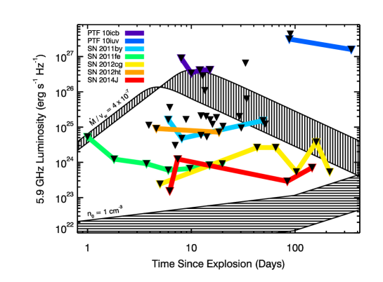
Figure 1.— 5.9 GHz upper limits from the Jansky VLA (downward facing black triangles), compared with models for a thermonuclear SN interacting with CSM (black hatched regions). SNe that are observed at multiple epochs are connected with colored solid lines (see Tables 2 and 4). Observations that were carried out at frequencies differing from 5.9 GHz were normalized to 5.9 GHz assuming an optically-thin synchrotron spectral index, $\alpha=-1$. The model light curve that is vertically hatched and peaks around Day 10 is for a wind-stratified CSM with $\dot{M}/v_{w}=4\times 10^{-7}~{}{{{\rm M}_{\odot}\ {\rm yr}^{-1}}\over{{\rm 100\ km\ s}^{-1}}}$ assuming $\epsilon_{e}=0.1$, $M_{\rm ej,Ch}=1$, and $E_{\rm K,51}=1$; its finite width shows the effect of varying $\epsilon_{B}$ between 0.01–0.1. The horizontally hatched light curve model that monotonically increases is for a uniform density CSM with $n_{0}=1$ cm^-3, $\epsilon_{e}=0.1$, $M_{\rm ej,Ch}=1$, and $E_{\rm K,51}=1$—again, its width is set to span $\epsilon_{B}=0.01-0.1$.

We further present archival observations of a sample of 31 older, mostly unpublished thermonuclear SNe observed with the historical VLA, obtained between 1998–2009 (Table 3). The VLA archive was searched for observations of nearby, bright, or particularly interesting thermonuclear SNe obtained within one year of explosion and providing more than 5 minutes on source. In particular, we searched the VLA archive for observations of (i) all SNe Ia listed on the Rochester Astronomy Supernova page as discovered between 1995–2009 and $\lesssim$15 mag at optical maximum; (ii) all SNe Iax catalogued by Foley et al. (2013); (iii) all Ca-rich SNe identified in Perets et al. (2010); (iv) SNe Ia potentially exceeding the Chandrasekhar mass as listed in Taubenberger et al. (2011); and (v) “non-PTF” SNe Ia-CSM as catalogued by Silverman et al. (2013).

Finally, we re-consider 29 SNe Ia with radio limits observed with the VLA in the first year following explosion, published in the refereed literature (Table 4). 26 of these are from Panagia et al. (2006), which tend to be bright ($\leq$ 14 mag at maximum) events that occurred over the period 1980–2003. Limits on three additional events of particular interest were published in Kasliwal et al. (2012); Dilday et al. (2012), and Cao et al. (2015); these limits are also plotted in Figure 1, as they were obtained with the upgraded Jansky VLA.

The complete sample of 85 thermonuclear SNe observed with the VLA is presented in Table 1. The SN positions listed in Table 1 originate from the “List of Supernovae” published by the IAU Central Bureau for Astronomical Telegrams. Host galaxy distances and morphological types are from the NASA Extragalactic Database (NED). We used the average “redshift-independent distance” measurement in NED if available as of June 2015; otherwise, we used the Galactocentric GSR distance from NED, which assumes $H_{0}=73$ km s^-1 Mpc^-1. For three particularly nearby SNe Ia, high-quality distance estimates originating from specific publications were used—SN 2011fe in M 101 (Shappee & Stanek, 2011), SN 2014J in M 82 (Dalcanton et al., 2009), and SN 1986G in NGC 5128 (Harris et al., 2010). The dates of optical $B$-band maximum for SNe were estimated from published data, as referenced in Table 1. Where public light curves are not available, we estimate the time of explosion from spectral information (occasionally from classification circulars).

2.2. Categorization of supernovae

The spectroscopic diversity of thermonuclear SNe is well established and extensively studied (e.g., Branch et al., 2006; Perets et al., 2010; Foley et al., 2013; Parrent et al., 2014; White et al., 2015). Recently, there has arisen evidence for a diversity of progenitors, and the nature of SN progenitors is likely aligned with spectroscopic categorization (e.g., Perets et al., 2010; Foley et al., 2012a, 2013; Maguire et al., 2013). Therefore, we divide the thermonuclear SNe observed with the VLA into nine categories, to provide limits on the radio emission from particular sub-types:

1. “Iax” low-luminosity explosions that resemble SN 2002cx (Foley et al., 2013);

2. Low-luminosity events of which SN 2002es is the prototype (Ganeshalingam et al., 2012);

3. “Ca-rich” low-luminosity events of which SN 2005E is the prototype (Perets et al., 2010; Kasliwal et al., 2012);

4. “Cool”/faint SNe Ia that resemble SN 1991bg (Benetti et al., 2005; Branch et al., 2006);

5. “Broad-line”/high velocity SNe Ia, which display a high temporal velocity gradient as defined by Benetti et al. (2005). SN 1984A is a classic example (Branch et al., 2006);

6. “Core-normal” events with a low temporal velocity gradient, of which SN 1994D is the prototype (Benetti et al., 2005; Branch et al., 2006);

7. “Shallow-Silicon” SN 1999aa-like SNe Ia, which also show low temporal velocity gradients (Benetti et al., 2005; Branch et al., 2006);

8. Luminous SNe Ia which are candidate super-Chandrasekhar-mass explosions (e.g., SN 2003fg; Howell et al. 2006);

9. “Ia-CSM”, which are SNe Ia that develop hydrogen emission lines, signalling circumstellar interaction (e.g., SN 2005gj; Silverman et al. 2013).

We assigned each VLA-observed thermonuclear SN one of these categories, based upon published spectra and circulars. The thermonuclear SNe are listed under their respective categories in Table 1.

In some cases (e.g., when spectroscopy was only obtained after maximum light), it was difficult to differentiate between core-normal and broad-line classifications. In these cases, we categorized the SNe as core-normal and marked them with a superscript in Table 1. In addition, several of the SNe in our sample are hybrid cool/normal SNe Ia; these are also distinguished in Table 1 with a superscript.

While the time of optical maximum light is usually well measured, it is the time since explosion that defines the properties of the radio evolution. To this end, we estimate the explosion time with respect to maximum light (i.e. the rise time of the $B-$band light curve) separately for the different classes as:

• Iax: $t_{\rm rise}\approx$15 days (Foley et al., 2013; Stritzinger et al., 2014);

• 02es-like: we only consider one member of this class—iPTF 14atg—and its rise time was measured to be 18.8 days (Cao et al., 2015);

• Ca-rich: $t_{\rm rise}\approx$12 days (Kasliwal et al., 2012);

• Cool: $t_{\rm rise}\approx 13$ days (Ganeshalingam et al., 2011);

• Broad-line: $t_{\rm rise}\approx 16.6$ days (Ganeshalingam et al., 2011);

• Core-normal: $t_{\rm rise}\approx 18.0$ days (Ganeshalingam et al., 2011);

• Shallow-silicon: $t_{\rm rise}\approx 18.1$ days (Ganeshalingam et al., 2011);

• Super-Chandrasekhar: $t_{\rm rise}\approx 24$ days (Scalzo et al., 2010; Silverman et al., 2011);

• Ia-CSM: $t_{\rm rise}\approx 30$ days (Silverman et al., 2013).

To calculate the time elapsed between explosion and VLA observation (as listed in Tables 2–4), we utilize the estimates of $B$-band optical maximum from Table 1, and these type-dependent rise times.

3. Observations

Observations with the upgraded VLA (2010 and after) were obtained in the standard continuum observing mode. During the early VLA commissioning phase, this provided a bandwidth of $2\times 128$ MHz, and later $2\times 1024$ MHz of bandwidth (programs AS1015, AS1058, 11B-177, 11B-217, 12A-482, 13B-454, and TOBS0008). The details of the observations are presented in Table 2. Most observations were obtained at C band (4–8 GHz). We utilized the maximum bandwidth available at the time of each observation (see Table 2) and recorded four polarization products. The observations were typically 1 hr in total duration resulting in $\sim 35-40$ min on source. For phase calibration, we used a complex gain calibrator source within $\sim 10$ degrees of each SN. For flux and bandpass calibration, one of 3C48, 3C147, or 3C286 was observed in each block.

The data were edited, calibrated, and imaged using standard routines in the Astronomical Image Processing System (AIPS; Greisen 2003). Each sideband was imaged individually. Individual sidebands were checked for a detection at the SN position, and when none was found, maximal sensitivity was achieved by smoothing the higher-frequency image to the resolution of the lower-frequency image, and then averaging the images from the two sidebands together. For those SNe observed in more compact configurations and located near regions of detectable diffuse host galaxy emission, we used a limited uv range in imaging the SN field to reduce contamination on short baselines. In some cases where there was significant contaminating flux from a nearby source, we chose to only use the higher-frequency sideband; these are marked in Table 2 as observations with diminished bandwidth (i.e., PTF 10icb, SN 2011iv, SN 2011iy, SN 2014J). Our reduced images typically reach expectations for the theoretical noise limit, except in cases where there are bright continuum sources nearby.

Observations with the pre-upgrade (pre-2010) VLA span frequencies 1.4–22.5 GHz, but were mostly commonly obtained at 4.8 or 8.4 GHz to maximize sensitivity (Tables 3 and 4). They were acquired in standard continuum mode ($2\times 43$ MHz bandwidth). These observations are typically $\sim$5 times less sensitive than the post-upgrade observations, and often tackle thermonuclear SNe at greater distances, so they are significantly less constraining than the post-upgrade VLA observations in terms of radio luminosity.

We did not detect positionally coincident radio emission from any of the thermonuclear SNe in our sample. To determine upper limits on the radio flux density, we measured the image rms noise ($\sigma_{\nu}$) and the flux density ($S_{\nu}$) at the optical SN position. Upper limits considered in this study are of 3$\sigma$ significance. In cases where the flux density measured at the SN position is a positive value, we calculate the flux density upper limit as $S_{\nu}+3\sigma_{\nu}$; where the flux density at the SN position is negative, we set the flux density upper limit to $3\sigma_{\nu}$. Limits taken from the literature, as listed it Table 4, are simply $3\sigma_{\nu}$, as these publications do not provide flux densities at the positions of the SNe. Luminosity upper limits presented in Tables 2, 3, and 4 assume the distances listed in Table 1. These luminosity constraints are translated into upper limits on the density of CSM (also listed in Tables 2–4) as described in Section 5.

4. Synchrotron emission from thermonuclear supernovae

While optical observations of young freely-expanding SNe probe the expanding ejecta, radio observations trace the dynamical interaction of the fastest ejecta with the circumstellar environment. This interaction accelerates particles to relativistic speeds and amplifies the magnetic field in the shocked region, producing radio synchrotron emission (Chevalier, 1982b). We make the common assumption that the energy densities in both relativistic particles and magnetic field scale with the post-shock energy density, $\sim\rho_{\rm CSM}\,v_{s}^{2}$, where $\rho_{\rm CSM}$ is the mass density of the CSM being impacted by the shock at time of observation, and $v_{s}$ is the blast wave velocity (Chevalier, 1996). Therefore, a SN will be more radio luminous if it has a fast shock velocity or expands into CSM of high density.

This interaction between SN blast and the surrounding medium leads to a double shock system in which the forward shock plows through the CSM while the reverse shock travels into and decelerates the ejecta (Chevalier, 1982b). A contact discontinuity at radius, $R_{c}$, divides the forward-shocked CSM from the reverse-shocked ejecta, and the total shocked region at any time is bounded by the locations of the forward and reverse shocks. The temporal evolution of $R_{c}$ is described by a self-similar solution determined by the density profile of the SN ejecta, $\rho_{\rm SN}$, and that of the local CSM, $\rho_{\rm CSM}$ (Chevalier, 1982a).

The radio properties of thermonuclear SNe may be reasonably predicted from radio observations and detailed modeling of well-observed SNe Ib/c. These explosions are produced through the gravitational collapse of massive stars that have ejected their hydrogen envelopes prior to explosion (Chevalier & Fransson, 2006). Since both white dwarfs and Type Ib/c progenitors lack a massive stellar envelope, the blast waves of both thermonuclear SNe and Ib/c are unencumbered and reach similar high velocities of $\overline{v}_{s}\approx 0.1c-0.3c$. As described below, making the reasonable assumption that the properties of accelerated electrons and amplified magnetic field are similar for thermonuclear SNe and Ib/c explosions, we construct models for the radio emission from SNe Ia and other white dwarf SNe.

4.1. A model for the ejecta profile

The unshocked SN ejecta expand freely and homologously, such that the expansion velocity ($v$) at some radius ($r$) in the ejecta observed at a time ($t$) after explosion is $v=r/t$. The early photospheric emission from SNe Ia points to an exponential density distribution for the inner, denser ejecta layers of exploded white dwarfs, $\rho_{\rm SN}({\rm inner})\propto{\rm e}^{-v}$ (i.e., the W7 model; Nomoto et al. 1984). This profile is supported by observations of the reverse shock-heated ejecta in Type I Galactic SN remnants (e.g., Hamilton & Fesen 1988; Itoh et al. 1988; Dwarkadas & Chevalier 1998). Meanwhile, a steep power-law density profile has been suggested for the outer ejecta layers, $\rho_{\rm SN}({\rm outer})\propto v^{-n}$, based on theoretical expectations for the explosion of a polytrope (Colgate & McKee, 1969; Chevalier, 1982b; Matzner & McKee, 1999; Nakar & Sari, 2010). Combining these two profiles, we construct a radial density profile for thermonuclear SN ejecta characterized by a relatively flat, exponential density profile at low velocities (inner ejecta) and a steep power-law density profile at high velocities (outer ejecta). A break velocity, $v_{b}$, divides the two regimes. Our analytic model for the ejecta density profile matches the results of SN Ia simulations well (Figure 2).

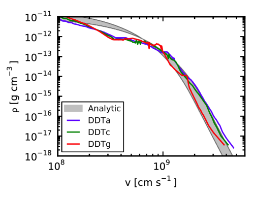
Figure 2.— Our analytic form of the radial density profile for SN Ia ejecta (grey band), compared with ejecta profiles from SN Ia simulations (colored lines). The width of the grey band spans $E_{\rm K,51}=0.8-1.5$ and assumes $M_{\rm ej,Ch}=1$. The red, green, and blue lines represent one-dimensional hydrodynamic+nucleosythesis simulations of SNe Ia from Badenes et al. (2003, 2005, 2008). They correspond to delayed detonations with energies, $E_{\rm K,51}=0.8$ (DDTg; red), $E_{\rm K,51}=1.2$ (DDTc; green), and $E_{\rm K,51}=1.4$ (DDTa; blue); all simulations assume $M_{\rm ej,Ch}=1$. These profiles all correspond to $10^{6}$ s after explosion, assuming free expansion and no CSM interaction.

We adopt the formalism of Dwarkadas & Chevalier (1998) for the inner ejecta profile,

$$\rho_{\rm SN}({\rm inner})=\rho_{0,{\rm in}}\ e^{-v/{v_{e}}}\ t^{-3}$$ (1)

where

$$\rho_{0,{\rm in}}\approx\left(7.67\times 10^{6}~{}\rm g~{}cm^{-3}\right)M_{\rm ej,Ch}^{5/2}~{}E_{\rm K,51}^{-3/2}$$ (2)

$$v_{e}\approx\left(2.44\times 10^{8}~{}\rm cm~{}s^{-1}\right)~{}M_{\rm ej,Ch}^{-1/2}~{}E_{\rm K,51}^{1/2}.$$ (3)

Here, $E_{\rm K,51}$ is the kinetic energy of the SN in units of $10^{51}$ erg, and $M_{\rm ej,Ch}$ is the ejecta mass in units of the Chandrasekhar mass, 1.4 M_⊙.

We characterize the outer layers of the ejecta with a power-law profile appropriate for a compact progenitor star derived from the harmonic mean models of Matzner & McKee (1999, Equation 46 and Table 5). The case of interest here is a $\gamma=4/3$ polytrope, which is appropriate to a relativistic white dwarf approaching the Chandrasekhar mass. In this framework,

$$\rho_{\rm SN}({\rm outer})=\rho_{0,{\rm out}}~{}v^{-10.18}~{}t^{-3}$$ (4)

where

$$\rho_{0,{\rm out}}\propto M_{\rm ej}^{-2.59}~{}E_{\rm K,51}^{3.59}$$ (5)

as shown by Berger et al. (2002) and Chevalier & Fransson (2006) for Wolf-Rayet star explosions.

Equating the slopes and normalization of the profiles for the inner and outer ejecta regions we find the location of the break velocity:

$${\rm v}_{b}\approx(2.48\times 10^{9}~{}{\rm cm~{}s^{-1}})~{}M_{\rm ej,Ch}^{-1/2}~{}E_{\rm K,51}^{1/2}$$ (6)

and the density normalization of the outer ejecta (in cgs units):

$$\rho_{0,{\rm out}}\approx(1.3\times 10^{98}~{}{\rm g~{}cm^{-3}})~{}M_{\rm ej,Ch}^{-2.59}~{}E_{\rm K,51}^{3.59}.$$ (7)

Our default assumption in this paper are the often-assumed parameters for SNe Ia, $M_{\rm ej,Ch}=1$, $E_{\rm K,51}=1$. We also apply our model to the ejecta of sub-luminous SN Iax and Ca-rich explosions, but note that in these cases, $E_{\rm K,51}$ and $M_{\rm ej,Ch}$ are both $<1$ (Perets et al., 2010; Foley et al., 2013); implications are discussed further in §4.5 and §6.

4.2. Self-similar solutions for blast wave dynamics

The initial interaction between the SN ejecta and the surrounding medium occurs at the outermost reaches of the ejecta which expand at the highest velocities, reaching great speeds because they were accelerated by the SN shock traveling down the steep density gradient at the outer edge of the white dwarf (Sakurai, 1960). This interaction is self-similar, as described in Chevalier (1982a). We parameterize the radial density profile of the outer SN ejecta as $\rho_{\rm SN}\propto r^{-n}$, and that of the CSM as $\rho_{\rm CSM}\propto r^{-s}$. The CSM is characterized as $\rho_{\rm CSM}=A~{}r^{-s}$ where $A$ is a normalization constant. Here $s=0$ in the case of a constant density medium and $s=2$ for a stellar-wind stratified environment.

At a particular time $t$, the shock contact discontinuity is located at:

$$R_{c}=\left[\frac{C~{}\rho_{0,{\rm out}}}{A}\right]^{1/(n-s)}t^{(n-3)/(n-s)}$$ (8)

where $C$ is a constant that depends on the properties of the interaction region (Chevalier, 1982a). Self-similarity therefore imposes a strict relation between $n$, $s$ and the temporal evolution of the contact discontinuity radius, $R_{c}\propto t^{m}$, with $m=(n-3)/(n-s)$ (Chevalier, 1998).

We consider two specific self-similar solutions associated with uniform-density and wind-stratified CSM environments, respectively. In the case of a constant density medium, $s=0$, $C\approx 0.32$, and the ratio of the forward shock radius, $R_{FS}$, to that of the contact discontinuity is $R_{FS}/R_{c}\approx 1.13$ (see Table 1 of Chevalier 1982a). For a wind-stratified CSM, $s=2$, $C\approx 0.064$, and $R_{FS}/R_{c}\approx 1.24$.

For $n=10.18$ (Equation 4), we find $m\approx 0.71$ for $s=0$, and $m\approx 0.88$ for $s=2$. The radial evolution of the forward shock is thus given by

$$R_{FS}(s=0)\approx(14\times 10^{15}~{}{\rm cm})~{}M_{\rm ej,Ch}^{-0.25}~{}E_{\rm K,51}^{0.35}~{}n_{0}^{-0.10}~{}t_{10}^{0.71}$$ (9)

$$R_{FS}(s=2)\approx(5.0\times 10^{15}~{}{\rm cm})~{}M_{\rm ej,Ch}^{-0.32}~{}E_{\rm K,51}^{0.44}~{}A_{\star}^{-0.12}~{}t_{10}^{0.88}$$ (10)

where $t_{10}$ is the time since explosion normalized to 10 days, $n_{0}$ is the CSM particle number density normalized to 1 cm^-3 in the uniform density case ($s=0$), and $A_{\star}=A/5\times 10^{11}~{}\rm g~{}cm^{-1}$. $A_{\star}=1$ corresponds to $\dot{M}/v_{w}=10^{-6}~{}{{{\rm M}_{\odot}\ {\rm yr}^{-1}}\over{{\rm 100\ km\ s}^{-1}}}$ (Chevalier & Fransson, 2006). Here and throughout this paper we assume a solar abundance for the CSM with mean molecular weight, $\mu=1.4$.

The velocity of the forward shock directly follows as $v_{s}\approx 0.71~{}R_{FS}/t$ for $s=0$, and $v_{s}\approx 0.88~{}R_{FS}/t$ in the case of $s=2$. For $M_{\rm ej,Ch}=1$, $E_{\rm K,51}=1$, and fiducial CSM densities ($n_{0}=1$, $A_{\star}=1$), the forward shock velocity is $0.38\,c$ and $0.17\,c$, respectively, at $t=10$ days since explosion.

We note that this self-similar solution only applies while the reverse shock is interacting with the outer layers of the ejecta distribution characterized by $v\gtrsim v_{b}$. The location of the reverse shock during this time trails just behind the contact discontinuity radius, with $R_{RS}/R_{c}\approx 0.97$ for $s=0$, and $R_{RS}/R_{c}\approx 0.98$ ($s=2$; Chevalier 1982a). For the fiducial CSM densities and explosion parameters adopted above, the reverse shock begins to probe the inner, exponentially-distributed material on a timescale of $\sim 5$ years after explosion, and the subsequent evolution of the interaction is modified (see Dwarkadas & Chevalier 1998 for further discussion). Thus the self-similar model is appropriate during the timescale of our radio observations (i.e. days to one year after explosion, see Tables 2–4).

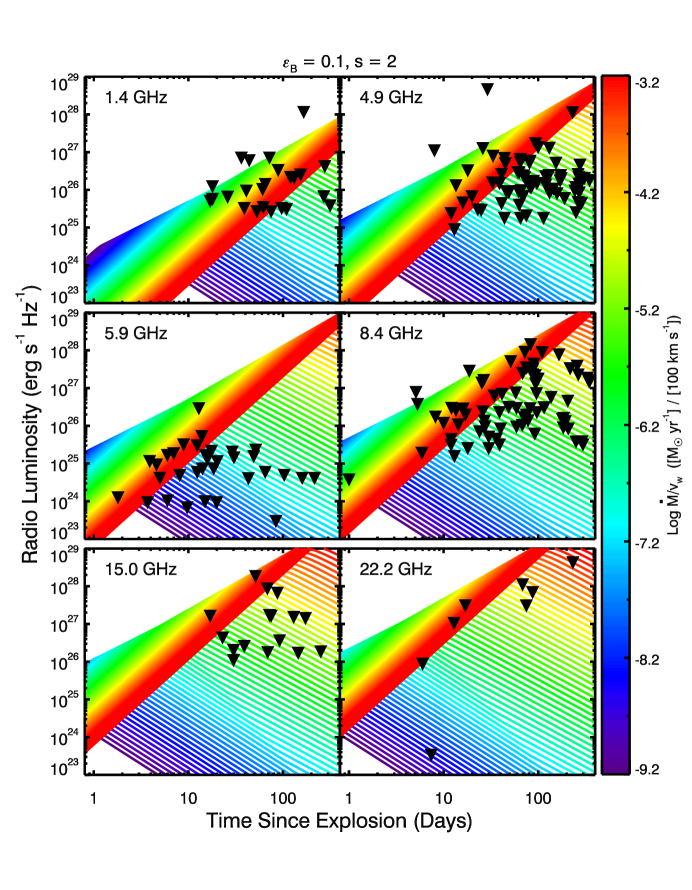
Figure 3.— Each panel shows a grid of radio light curve models at a distinct frequency (marked top left), assuming $\epsilon_{B}=0.1$, $\epsilon_{e}=0.1$, $M_{\rm ej,Ch}=1$, $E_{\rm K,51}=1$, and $s=2$. The model grids span a range of $\dot{M}/v_{w}$ values ($\dot{M}/v_{w}=6\times 10^{-10}-6\times 10^{-4}~{}{{{\rm M}_{\odot}\ {\rm yr}^{-1}}\over{{\rm 100\ km\ s}^{-1}}}$) with spacing of 0.1 dex, as described in Section 5, with purple-blue models corresponding to low $\dot{M}/v_{w}$ values and red models to high $\dot{M}/v_{w}$. Observed 3$\sigma$ upper limits at each frequency are overplotted as black triangles.

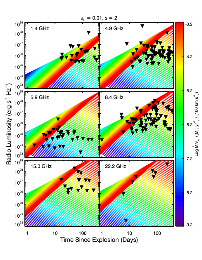
Figure 4.— Each panel shows a grids of radio light curve models at a distinct frequency (marked top left), assuming a more conservative $\epsilon_{B}=0.01$ (compared to $\epsilon_{B}=0.1$ in Figure 3) and retaining $\epsilon_{e}=0.1$, $M_{\rm ej,Ch}=1$, $E_{\rm K,51}=1$, and $s=2$. The model grid and color scheme represent the same range of $\dot{M}/v_{w}$ values as in Figure 3. Observed 3$\sigma$ upper limits at each frequency are overplotted as black triangles.

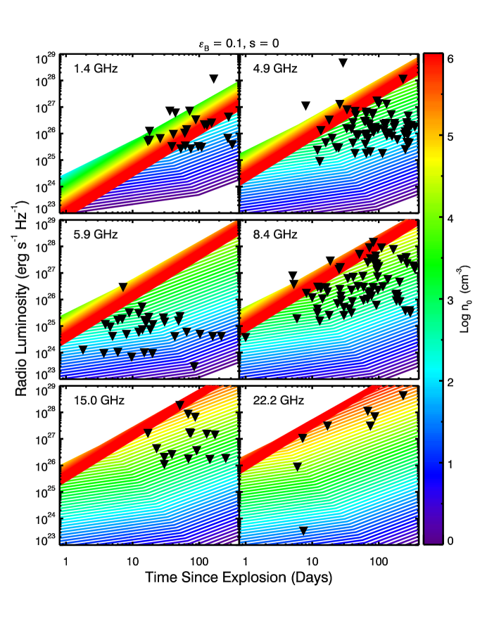
Figure 5.— Each panel shows a grids of radio light curve models at a distinct frequency (marked top left), assuming $\epsilon_{B}=0.1$, $\epsilon_{e}=0.1$, $M_{\rm ej,Ch}=1$, $E_{\rm K,51}=1$, and $s=0$. The model grids span a range of $n_{0}$ values ($n_{0}=1-10^{6}$ cm^-3) with resolution of 0.1 dex, with purple-blue models corresponding to low $n_{0}$ values and red models to high $n_{0}$. Observed 3$\sigma$ upper limits at each frequency are overplotted as black triangles.

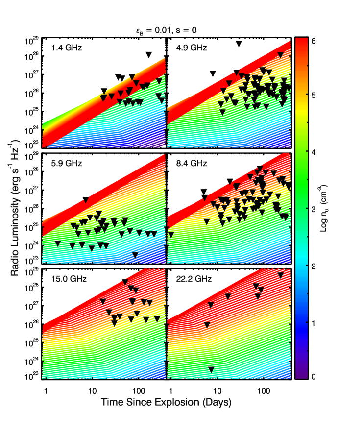
Figure 6.— Each panel shows a grids of radio light curve models at a distinct frequency (marked top left), assuming a more conservative $\epsilon_{B}=0.01$ (compared to $\epsilon_{B}=0.1$ in Figure 5) and retaining $\epsilon_{e}=0.1$, $M_{\rm ej,Ch}=1$, $E_{\rm K,51}=1$, and $s=0$. The model grid and color scheme represent the same range of $n_{0}$ values as in Figure 5. Observed 3$\sigma$ upper limits at each frequency are overplotted as black triangles.

4.3. Magnetic field amplification and acceleration of relativistic particles

As the forward shock barrels outward into the CSM, electrons are shock-accelerated to relativistic velocities and magnetic fields are amplified through turbulence (Chevalier, 1982b). We assume that constant fractions of the post-shock energy density ($\rho_{\rm CSM}~{}v_{s}^{2}$) are shared by the relativistic electrons ($\epsilon_{e}$), protons ($\epsilon_{p}$), and amplified magnetic fields ($\epsilon_{B}$; Chevalier 1998; Chevalier & Fransson 2006).

The strength of the amplified magnetic field in the post-shock region is

$$B=\sqrt{8\pi\,\epsilon_{B}\,\rho_{\rm CSM}\,v_{s}^{2}}$$ (11)

in cgs units ($B$ in units of G). The magnetic field strength decreases with time and shock radius, because $v_{s}$ is decreasing—and in the case of wind-stratified CSM, $\rho_{\rm CSM}$ is also decreasing. Combining Equation 11 with Equations 9 and 10, we find

$$B(s=0)\approx(0.028\ {\rm G})~{}\epsilon_{B,-1}^{0.5}~{}n_{0}^{0.40}~{}M_{\rm ej,Ch}^{-0.25}~{}E_{\rm K,51}^{0.35}~{}t_{10}^{-0.29}$$ (12)

$$B(s=2)\approx(1.3\ \rm G)~{}\epsilon_{B,-1}^{0.5}~{}A_{\star}^{0.5}~{}t_{10}^{-1}.$$ (13)

where $\epsilon_{B,-1}$ is normalized to a fiducial value, $\epsilon_{B}=0.1$.

The accelerated electrons populate a high velocity tail that extends beyond the thermal distribution. Above a minimum energy, $E_{m}\equiv\gamma_{m}\,m_{e}\,c^{2}$ (where $\gamma_{m}$ is the minimum Lorentz factor of the electrons), the shocked electrons are characterized by a power-law distribution of energies, $N(E>E_{m})=N_{0}\,E^{-p}$. Observations of other stripped envelope supernovae of Type Ib/c have measured $p=3$ from the optically-thin synchrotron spectral index (e.g., Weiler et al., 1986; Berger et al., 2002; Soderberg et al., 2005, 2006).

In this framework (Chevalier, 1998), the normalization of the electron distribution is:

$$N_{0}=(p-2)~{}\epsilon_{e}~{}\rho_{\rm CSM}~{}v_{s}^{2}~{}E_{m}^{p-2}.$$ (14)

The minimum electron energy is coupled to the shock velocity as (Chevalier & Fransson, 2006):

$$E_{m}=1.2\,\frac{(p-2)~{}\epsilon_{e}~{}m_{p}~{}v_{s}^{2}}{(p-1)~{}\eta}.$$ (15)

where $\eta$ is the compression factor of material in the post-shock region. This equation holds when $E_{m}>m_{e}c^{2}$; otherwise we set $E_{m}$ to the electron rest mass energy ($\gamma_{m}=1$).

Combining Equations 9, 10 and 15, we derive expressions for the electron minimum Lorentz factor for white dwarf explosions within constant or wind-stratified CSM environments:

$$\gamma_{m}(s=0)\approx 32.9~{}\frac{\epsilon_{e,-1}}{\eta}~{}\frac{(p-2)}{(p-1)}~{}M_{\rm ej,Ch}^{-0.50}~{}E_{\rm K,51}^{0.70}~{}n_{0}^{-0.20}~{}t_{10}^{-0.58}$$ (16)

$$\gamma_{m}(s=2)\approx 6.3~{}\frac{\epsilon_{e,-1}}{\eta}~{}\frac{(p-2)}{(p-1)}~{}M_{\rm ej,Ch}^{-0.64}~{}E_{\rm K,51}^{0.88}~{}A_{\star}^{-0.24}~{}t_{10}^{-0.24}$$ (17)

where $\epsilon_{e.-1}$ is normalized to a fiducial value, $\epsilon_{e}=0.1$. For the fiducial values considered here, $\gamma_{m}$ is larger than unity on timescales of days to weeks after explosion. Henceforth, we assume $\eta=4$, as for a non-relativistic strong shock.

The relativistic electrons accelerated to $\gamma_{m}$ and beyond gyrate in the amplified magnetic field and produce synchrotron emission at a characteristic frequency, $\nu_{m}=\gamma_{m}^{2}(eB/2\pi m_{e}c)$. We find characteristic synchrotron frequency, $\nu_{m}\sim 10^{6}$ Hz at $t=10$ days for both the constant density and wind stratified scenarios, and this frequency decays as $\nu_{m}\propto t^{-1.5}$. Thus $\nu_{m}$ is well below the observed radio band on the timescale of our observations. The resultant non-thermal radio emission from the relativistic electron population results in a simple power-law synchrotron spectrum when optically thin, $F_{\nu}\propto\nu^{\beta}$ with $\beta=-(p-1)/2$.

4.4. Radio luminosity evolution

Synchrotron self-absorption by emitting electrons within the shock interaction region gives rise to a low-frequency turnover that yields a spectral peak, $\nu_{p}$, observed in Type Ib/c supernovae (Chevalier, 1998). In Type I supernovae, $\nu_{p}$ is equivalent to the synchrotron self-absorption frequency, since external free-free absorption does not contribute significantly (Chevalier, 1998; Chevalier & Fransson, 2006). We note that Panagia et al. (2006) assume that free-free absorption is the dominant source of opacity in the radio light curves of SNe Ia, justified by their assumed shock velocity of 10,000 km s^-1, which is significantly lower than the thermonuclear SN blast wave velocity derived here. For the fast SN blast waves described by Equations 9 and 10, the importance of free-free absorption is negligible compared to synchrotron self absorption.

Above $\nu_{p}$, synchrotron emission is optically thin and the flux density scales as $F_{\nu}\propto\nu^{-1}$ (for $p=3$). Below $\nu_{p}$, the emission is optically thick to synchrotron self-absorption, and the spectrum scales as $F_{\nu}\propto\nu^{5/2}$. As the blast wave expands, the optical depth to synchrotron self-absorption decreases and $\nu_{p}$ cascades to lower frequencies. The temporal and spectral evolution of the radio signal is therefore fully determined by the blast wave velocity and the density of the local environment.

Drawing from Equation 1 of Chevalier (1998), we find for $p=3$, the synchrotron flux density at observed frequency $\nu$, is:

$$F_{\nu}\approx 5.31\times 10^{-31}~{}R_{FS}^{2}~{}D^{-2}~{}B^{-1/2}~{}\nu^{5/2}\left[1-e^{-\left(\frac{\nu}{\nu_{1}}\right)^{-7/2}}\right]$$ (18)

in cgs units. Here, $D$ is the distance to the supernova and $\nu_{1}$ is the asymptotic peak frequency joining the optically thick and thin regimes. As the supernova expands and ages, $\nu_{1}$ decreases as:

$$\nu_{1}\approx(4.76\times 10^{7}~{}{\rm Hz})~{}R_{FS}^{2/7}~{}f^{2/7}~{}N_{0}^{2/7}~{}B^{5/7}.$$ (19)

defining the frequency at which the optical depth to synchrotron self-absorption is unity. Here, $f$ is the fraction of the spherical volume of the supernova blast which is emitting synchrotron radiation (i.e., $f=1-[R_{RS}/R_{FS}]^{3}$, assuming the radio emission fills the region between the forward shock and the reverse shock). For $s=0$, the solutions of Chevalier (1982a) yield $f=0.38$, while for $s=2$, $f=0.50$. We note that the observed peak frequency ($\nu_{p}$) is slightly displaced from $\nu_{1}$ due to exponential smoothing of the two regimes; for $p=3$ this shift is $\nu_{p}\approx 1.14~{}\nu_{1}$. As described in Chevalier (1998), the expressions for $F_{\nu}$ and $\nu_{1}$ make use of the synchrotron constants applicable for the case of $p=3$ from Pacholczyk (1970), specifically $c_{1}=6.27\times 10^{18}$, $c_{5}=7.52\times 10^{-24}$, and $c_{6}=7.97\times 10^{-41}$.

For low density environments ($n_{0}\lesssim 1$, $A_{\star}\lesssim 1$), the effects of synchrotron self-absorption in the centimeter band are minimized such that the optically thin regime is applicable at most times. In this scenario, the synchrotron emission may be simplified as:

$$F_{\nu}\approx 3.95\times 10^{-4}~{}R_{FS}^{3}~{}f~{}D^{-2}~{}N_{0}~{}B^{2}~{}\nu^{-1}~{}\rm erg~{}cm^{-2}~{}s^{-1}~{}Hz^{-1}.$$ (20)

Sample light curves are shown in Figure 1 for $A_{\star}=0.4$ and $n_{0}=1$ cm^-3, assuming $\epsilon_{e}=0.1$, $\epsilon_{B}=0.1$, $M_{\rm ej,Ch}=1$, and $E_{\rm K,51}=1$.

The properties of the CSM density profile and the forward shock evolution together determine the temporal behavior of the optically thin radio flux density. For $s=0$ and $\gamma_{m}>1$, the flux density rises with time as $F_{\nu}\propto t^{0.39}$; once $\gamma_{m}=1$, the flux density evolution steepens to $F_{\nu}\propto t^{0.97}$ (visible as a kink in the model light curve of Figure 1 with $n_{0}=1$ cm^-3 around 100 days after explosion). Meanwhile for $s=2$, the optically-thin scaling is $F_{\nu}\propto t^{-1.60}$ when $\gamma_{m}>1$; later, when $\gamma_{m}$ bottoms out at unity, then $F_{\nu}\propto t^{-1.36}$. Therefore, the temporal evolution of the optically-thin flux density can be used to estimate the density profile of the CSM.

4.5. Caveats and Complexities

As discussed by Horesh et al. (2012, 2013), the most significant uncertainty in converting radio luminosity to a density of the CSM is the efficiency of magnetic field acceleration, $\epsilon_{B}$. In the case of uniform density CSM and optically-thin synchrotron emission, the density derived from a given flux density will depend on $\epsilon_{B}$ as $n_{0}\propto\epsilon_{B}^{-0.91}$ when $\gamma_{m}>1$, and $n_{0}\propto\epsilon_{B}^{-0.77}$ when $\gamma_{m}=1$. For $s=2$ and $\gamma_{m}>1$, we find $A_{\star}\propto\epsilon_{B}^{-0.71}$, and when $\gamma_{m}$ converges to unity then $A_{\star}\propto\epsilon_{B}^{-0.61}$. In addition, as seen by comparing Figure 3 with Figure 4, and Figure 5 with 6, the synchrotron emission becomes optically thin faster for lower values of $\epsilon_{B}$.

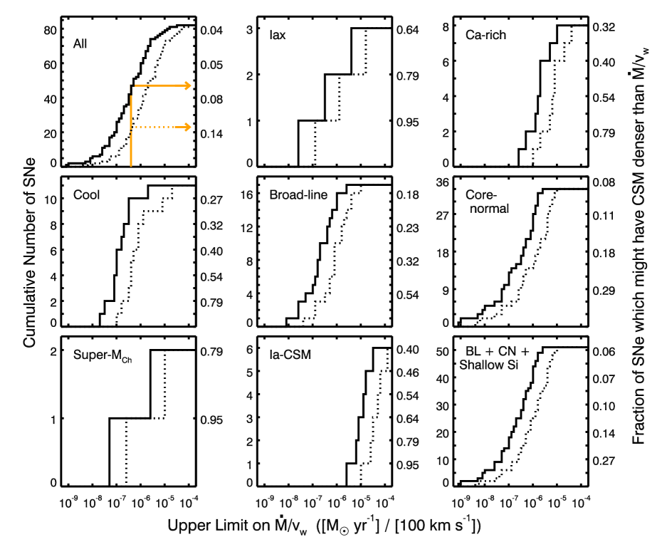
Figure 7.— Cumulative histograms of $\dot{M}/v_{w}$, normalized assuming $v_{w}$ = 100 km s^-1. Solid histograms assume $\epsilon_{B}=0.1$, while the dotted histograms assume $\epsilon_{B}=0.01$; all assume $s=2$, $M_{\rm ej,Ch}=1$, and $E_{\rm K,51}=1$. The top left panel includes all 82 thermonuclear SNe with $\dot{M}/v_{w}$ constraints, while the other eight panels divide these thermonuclear SNe into the sub-types described in Section 2.2. 02es-like and shallow-silicon supernovae are not shown in individual panels, as there is only one object in our sample of each of these sub-types. The bottom-right panel combines the sub-types of SNe Ia that are cosmologically useful (broad-line, core-normal, and shallow-silicon). The labels on the right side of the plot show what fraction of SNe in the sample might have surroundings denser than $\dot{M}/v_{w}$, based off simple binomial statistics at 2$\sigma$ significance. The orange lines in the top left panel illustrate that we constrain 47 thermonuclear SNe ($>$94% of all thermonuclear SNe) to have $\dot{M}/v_{w}<4\times 10^{-7}~{}{{{\rm M}_{\odot}\ {\rm yr}^{-1}}\over{{\rm 100\ km\ s}^{-1}}}$ assuming $\epsilon_{B}=0.1$ (orange solid line), and 23 thermonuclear SNe ($>$87% of all thermonuclear SNe) to meet this criterion if $\epsilon_{B}=0.01$ (orange dotted line).

Figure 8.— Cumulative histograms of $n_{0}$, assuming the CSM is uniform in density. Solid histograms assume $\epsilon_{B}=0.1$, while the dotted histograms assume $\epsilon_{B}=0.01$; all assume $s=0$, $M_{\rm ej,Ch}=1$, and $E_{\rm K,51}=1$. The top left panel includes all 82 thermonuclear SNe with $n_{0}$ constraints, while the other eight panels divide these thermonuclear SNe into the sub-types described in Section 2.2. 02es-like and shallow-silicon supernovae are not shown in individual panels, as there is only one object in our sample of each of these sub-types. The bottom-right panel combines the sub-types of SNe Ia that are cosmologically useful (broad-line, core-normal, and shallow-silicon). The labels on the right side of the plot show what fraction of SNe in the sample might have surroundings denser than $n_{0}$, based off simple binomial statistics at 2$\sigma$ significance.

Radio light curve models are also affected by the assumed values of SN ejecta mass and explosion energy. If we take conservatively low values of $M_{\rm ej,Ch}=0.1$ and $E_{\rm K,51}=0.1$, we find forward shock velocities of $0.13\,c$ and $0.29\,c$ at $t=10$ days since explosion for $A_{\star}=1$ and $n_{0}=1$ respectively. These blast wave velocities are high enough that synchrotron self absorption still dominates over free-free absorption. In the case of uniform density CSM and optically-thin synchrotron emission, the density derived from a given flux density will depend on ejecta mass and kinetic energy as $n_{0}\propto M_{\rm ej,Ch}^{2.05}\ E_{\rm K,51}^{-2.86}$ when $\gamma_{m}>1$, and $n_{0}\propto M_{\rm ej,Ch}^{1.35}\ E_{\rm K,51}^{-1.88}$ when $\gamma_{m}=1$. For $s=2$ and $\gamma_{m}>1$, we find $A_{\star}\propto M_{\rm ej,Ch}^{1.14}\ E_{\rm K,51}^{-1.57}$, and when $\gamma_{m}$ converges to unity then $A_{\star}\propto M_{\rm ej,Ch}^{0.59}\ E_{\rm K,51}^{-0.80}$. While these dependencies are quite strong, uncertainties in $M_{\rm ej,Ch}$ and $E_{\rm K,51}$ do not affect our constraints on $n_{0}$ and $A_{\star}$ as dramatically as they may first appear, because e.g., in low-luminosity thermonuclear explosions, both $M_{\rm ej,Ch}$ and $E_{\rm K,51}$ are suppressed (compared to fiducial SN Ia values). While decreasing the assumed $E_{\rm K,51}$ yields a less stringent constraint on $\rho_{\rm CSM}$, decreasing the assumed $M_{\rm ej,Ch}$ implies a stronger constraint, and therefore co-varying changes to $M_{\rm ej,Ch}$ and $E_{\rm K,51}$ largely counteract one another. The effects of assumed $M_{\rm ej,Ch}$ and $E_{\rm K,51}$ will be explored in more detail in §6.

The predicted radio emission is modified if cooling of the electrons steepens the spectrum, thus decreasing the emission as considered by Chevalier & Fransson (2006) for the case of SNe Ib/c. The case of synchrotron losses is analogous for the two supernova types and Equation 11 of Chevalier & Fransson (2006) shows that synchrotron losses are unimportant in both cases. For Inverse Compton losses, thermonuclear SNe have a higher peak optical luminosity, $\sim 10^{43}$ erg s^-1, than typical SNe Ib/c, but the lower ejecta mass leads to a larger distance of the relativistic electrons from the photosphere, so Inverse Compton losses are only of marginal importance, if any, at the time of optical maximum light.

5. Comparing Observations with Radio Light Curve Models

5.1. Upper Limits on CSM Density

The goal of the modelling described above is to translate our limits on the radio luminosity of thermonuclear SNe to constraints on the density of the CSM around thermonuclear SNe. We therefore calculated grids of radio light curves at all observed frequencies using these models, for comparison with observations.

For a wind CSM ($s=2$), we sample $\dot{M}/v_{w}$ space logarithmically with a resolution of 0.1 dex. The model grid spans mass loss rates $\dot{M}/v_{w}=6\times 10^{-10}-6\times 10^{-4}~{}{{{\rm M}_{\odot}\ {\rm yr}^{-1}}\over{{\rm 100\ km\ s}^{-1}}}$, assuming $M_{\rm ej}=M_{\rm ej,Ch}$, $E_{\rm K,51}=1$, and $\epsilon_{e}=0.1$.

The grid of wind CSM models at the most commonly observed frequencies is shown in Figures 3 and 4, with radio limits overplotted. The two figures are for different values of $\epsilon_{B}$. In Tables 2–4, we also list the upper limits on $\dot{M}/v_{w}$, normalized to $v_{w}=100$ km s^-1 and $\epsilon_{B}=0.1$. In the few cases where radio limits lie above the optically-thick locus of the model grid, they do not constrain the density of the CSM at all, and in these cases “N/A” is listed for the limit on $\dot{M}/v_{w}$.

At first glance, our constraints on $\dot{M}/v_{w}$ appear similar to those listed by Panagia et al. (2006) in their Table 3. However, they assume $v_{w}$ = 10 km s^-1, while our values of $\dot{M}/v_{w}$ are normalized to 100 km s^-1. Therefore, the constraints on $\dot{M}/v_{w}$ from the Panagia et al. model are a factor of $11.1\pm 6.2$ less constraining than the limits derived from our model. In addition, Panagia et al. (2006) quote 2$\sigma$ constraints on $\dot{M}/v_{w}$, while those presented here are 3$\sigma$, so the discrepancy in $\dot{M}/v_{w}$ is in fact somewhat larger than a factor of 11. Most of this discrepancy is attributable to Panagia et al.’s assumption of a slower blast wave ($v_{s}$ = 10,000 km s^-1); different assumptions about synchrotron opacity also affect the calculation. We note that Panagia et al. (2006) do not model their radio limits with uniform CSM.

Using our model of uniform-density CSM ($s=0$), we sample $n_{0}$ space logarithmically with a resolution of 0.1 dex, from $n_{0}=1$ cm^-3 to $n_{0}=10^{6}$ cm^-3. As for $s=2$, we assume $M_{\rm ej,Ch}=1$, $E_{\rm K,51}=1$, and $\epsilon_{e}=0.1$. These models are compared with our upper limits in Figures 5 and 6, for $\epsilon_{B}$ = 0.1 and 0.01, respectively. Upper limits on $n_{0}$ are also listed in Tables 2–4, assuming $\epsilon_{B}=0.1$ (again, “N/A” is listed if a limit sits above the optically-thick model locus).

It is clear that later observations, several years after explosion, will be significantly more constraining upon uniform density surroundings. Such later observations will be presented and discussed in a forthcoming publication. On the other hand, early observations are most constraining for a wind CSM.

It should also be noted that the assumption made in this paper, that the inner SN ejecta remain unshocked, is only valid out to time scales of one year if $n_{0}\lesssim$ 100 cm^-3 or $\dot{M}/v_{w}=10^{-5}~{}{{{\rm M}_{\odot}\ {\rm yr}^{-1}}\over{{\rm 100\ km\ s}^{-1}}}$. Our treatment of the highest CSM densities considered here is only valid at earlier times (out to Day 40 for $\dot{M}/v_{w}=10^{-4}~{}{{{\rm M}_{\odot}\ {\rm yr}^{-1}}\over{{\rm 100\ km\ s}^{-1}}}$, or Day 162 for $n_{0}=10^{3}$ cm^-3). SNe expanding into such dense CSM will also likely suffer free-free absorption. We mark observations that can not be completely described by the model of outer ejecta presented here—because the luminosity limit is not terribly deep or because the observation was taken at a relatively late time—with a superscript in Tables 3 and 4 (this situation does not apply to any of the observations in Table 2). Proper modeling of these highest CSM densities are outside the scope of this publication, but should be addressed in the future.

Cumulative histograms of $\dot{M}/v_{w}$ are shown in Figure 7 (normalized to $v_{w}=100$ km s^-1), for both our entire sample and broken up by thermonuclear SN sub-type. On the right side of each panel, we estimate the fraction of thermonuclear SNe that could have CSM denser than the plotted equivalent $\dot{M}/v_{w}$, and still be consistent with our measured limits at 2$\sigma$ significance. For example, take the case where we have a sample of 47 thermonuclear SNe which have all been constrained to have $\dot{M}/v_{w}<4\times 10^{-7}~{}{{{\rm M}_{\odot}\ {\rm yr}^{-1}}\over{{\rm 100\ km\ s}^{-1}}}$ (the average $\dot{M}/v_{w}$ for Galactic symbiotic binaries; see §5.2; Figure 7). There is a 95.5% (2$\sigma$) binomial probability of this occurrence if the probability of success on a single trial is 0.064. In other words, we estimate that $<$6.4% of thermonuclear SNe have $\dot{M}/v_{w}>4\times 10^{-7}~{}{{{\rm M}_{\odot}\ {\rm yr}^{-1}}\over{{\rm 100\ km\ s}^{-1}}}$. This simple analysis assumes that our observed thermonuclear SNe are representative of thermonuclear SNe as a whole (or of the sub-types, for the histograms broken down by type).

Similar cumulative histograms are shown in Figure 8 for uniform-density CSM. These limits are less constraining on progenitor models; we find that 13 SNe ($>$79% of all thermonuclear SNe at 2$\sigma$ significance) constrain $n_{0}<100$ cm^-3 for $\epsilon_{B}=0.1$. As previously discussed, future work presenting later radio observations of SNe Ia (1–100 years after explosion) will be more constraining on $n_{0}$.

5.2. Implications for Symbiotic Progenitors

The early-time limits on the radio luminosity presented here place significant constraints on symbiotic progenitors for thermonuclear SNe. Specifically, our limits constrain progenitors with red giant companions undergoing steady mass loss immediately preceding the thermonuclear SN. If there is a significant delay between the giant mass loss and the SN (Justham, 2011; Di Stefano et al., 2011), or if a cavity is excavated in the circumbinary material by e.g., an accretion-powered wind (Hachisu et al., 1999), the CSM would not be expected to follow the simple $\rho\propto r^{-2}$ we consider here, and would be better constrained by observations longer after SN explosion.

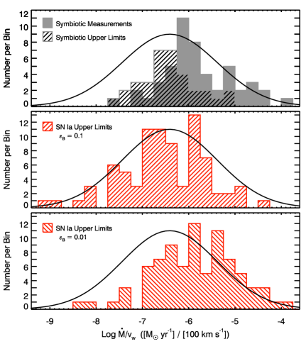
Figure 9.— Histograms comparing measurements and constraints on $\dot{M}/v_{w}$ for symbiotic binaries with upper limits for thermonuclear SNe, normalized to $v_{w}$ = 100 km s^-1. The top panel shows data for symbiotic binaries from Seaquist et al. (1993), with measurements as the gray shaded histogram and upper limits as the hatched histogram. The best-fit log-normal distribution to these data is shown as a black solid line. The middle panel shows the distribution of $\dot{M}/v_{w}$ upper limits for thermonuclear SNe as the red hatched histogram, assuming $M_{\rm ej,Ch}=1$, $E_{\rm K,51}=1$, and $\epsilon_{B}=0.1$; the fitted log-normal distribution for symbiotics is overplotted as a black solid line. The bottom panel is identical to the middle panel, except $\epsilon_{B}=0.01$ is assumed in the calculation of $\dot{M}/v_{w}$. We note that the amplitude of the log-normal fit to the Galactic symbiotics is arbitrary, and adjusted for diagnostic purposes.

Radio observations of Galactic symbiotic stars yield robust measurements of $\dot{M}/v_{w}$ in these systems, probing the ionized wind CSM via thermal free-free emission (Seaquist et al., 1984; Seaquist & Taylor, 1990; Seaquist et al., 1993). The distribution of $\dot{M}/v_{w}$ for symbiotic binaries is shown in Figure 9, presenting the catalog of Seaquist et al. (1993). Seaquist et al. note that their catalog contains “essentially every known symbiotic star observable with $\delta>-45^{\circ}$” as of 1993; the sample spans both S-type and D-type systems, and a range of IR and ultraviolet properties.

When a symbiotic system is detected at radio frequencies (filled gray histogram), its $\dot{M}/v_{w}$ was estimated by Seaquist et al. (1993) assuming a fully-ionized, spherically-symmetric wind CSM and the equations of Wright & Barlow (1975). In other cases, when a symbiotic binary is not detected, a 3$\sigma$ upper limit on its $\dot{M}/v_{w}$ was given by Seaquist et al. (1993), and is plotted in the top panel of Figure 9 as the hatched histogram. Note that the radio measurements of symbiotic stars constrain $\dot{M}/v_{w}$, as we also do for thermonuclear SNe here. While Seaquist et al. (1993) assume $v_{w}$ = 30 km s^-1 in their analysis, in our Figure 9 we have normalized their reported $\dot{M}/v_{w}$ to $v_{w}$ = 100 km s^-1, for consistency with the rest of our study. Seaquist et al. (1993) also note that their measurements of symbiotic $\dot{M}/v_{w}$ should be viewed as lower limits, because the red giant wind is only partially ionized in most systems. However, the total neutral + ionized $\dot{M}/v_{w}$ is probably within a factor of $\sim$2 of the estimates presented by Seaquist et al. (1993) and plotted in Figure 9.

We used these measurements to estimate the distribution of $\dot{M}/v_{w}$ for the known symbiotic systems. To do this, we used a Bayesian Markov Chain Monte Carlo technique to fit a log-normal distribution to both the measured $\dot{M}/v_{w}$ values and the censored data (upper limits on $\dot{M}/v_{w}$), assuming common uncertainties of 0.3 dex and flat priors. We find that the distribution of log($\dot{M}/v_{w}$) for Galactic symbiotic binaries has a best-fit model with a mean, $\mu=-6.41^{+0.14}_{-0.13}$ and standard deviation, $\sigma=1.03^{+0.13}_{-0.11}$ (top panel of Figure 9).

Our next step was to compare the collection of upper limits for the themonuclear SNe to the best-fit distribution for symbiotic binaries (middle and lower panels of Figure 9). To do this, we make the simplifying assumption that there are two populations of thermonuclear SNe: those with symbiotic progenitors that behave like the known symbiotics, and a second population of unspecific origin that does not produce radio emission detectable with current facilities. We generate Monte Carlo samples with a varying fraction $f$ drawn from the symbiotic population, then censor these data with the observed thermonuclear SN limits. We take the test statistic as the fraction of trials in which no SNe Ia would be detected (as observed).

For $\epsilon_{B}=0.1$, at the level of $p=0.05$, the maximum fraction of symbiotic progenitors allowable by our radio limits is $f=0.07$. At a more conservative $p=0.01$, this fraction is $f=0.10$. The corresponding $p=0.05$ and $p=0.01$ values for $\epsilon_{B}=0.01$ are $f=0.10$ and 0.16, respectively. Thus we conclude that no more than $\sim$10–15% of thermonuclear SNe have symbiotic progenitors comparable to Galactic binaries. A relatively high rate of such progenitors ($\sim 25$%), as inferred from other studies (Sternberg et al., 2011; Maguire et al., 2013), is inconsistent with our observations to a high degree of confidence.

Since this analysis is based on the population properties of SNe Ia, and the distribution of symbiotic mass loss rates is relatively broad, these constraints can continue to be improved with additional radio continuum observations. Since symbiotic progenitors appear to be relatively uncommon, a larger set of observations of modest depth would improve the constraints more than a smaller number of more sensitive observations or a focus on the nearest SNe.

6. Notes on Some Individual Sub-types and Sources

6.1. SNe Iax

Our constraints on $\rho_{\rm CSM}$ for SNe Iax assuming $M_{\rm ej,Ch}=1$ and $E_{\rm K,51}=1$ can be found in Figures 7 and 8, along with Tables 2 and 3. However, these low-luminosity explosions likely have significantly lower ejecta mass and explosion kinetic energy. Reasonable assumptions for the class are $M_{\rm ej,Ch}\approx 0.4$ ($\sim$0.5 M_⊙) and $E_{\rm K,51}\approx 0.1$ (Foley et al., 2013); detailed calculations on SN 2008ha imply even lower ejecta masses and energies in some cases (Foley et al., 2009, 2010; Valenti et al., 2009). SNe Iax and appropriately-scaled light curve models are shown in Figure 10.

Based on the pre-explosion detection of SN Iax 2012Z and claims that its companion may be a He star (Foley et al., 2013; McCully et al., 2014), the CSM of He stars is worth considering. He stars have been observed to have winds with $\dot{M}=10^{-11}-10^{-7}$ M_⊙ yr^-1 and $v_{w}$ = few hundred – few thousand km s^-1 (Jeffery & Hamann, 2010). Our limits from the pre-upgrade VLA are far from constraining of He star companions; we find $\dot{M}\lesssim{\rm few}\times 10^{-6}-10^{-4}$ M_⊙ yr^-1 for $v_{w}$ = 400 km s^-1, $M_{\rm ej,Ch}=0.4$, and $E_{\rm K,51}=0.1$. However, our Jansky VLA limit on SN 2012Z approaches the He star parameter space ($\dot{M}<2\times 10^{-7}$ M_⊙ yr^-1 for $v_{w}$ = 400 km s^-1, $M_{\rm ej,Ch}=0.36$, and $E_{\rm K,51}=0.1$). Future nearby SNe Iax are ideal targets for deep radio observations.

Figure 10.— 5.9 GHz upper limits for the four SNe Iax in our sample (downward facing black triangles), compared with models for a thermonuclear SN interacting with CSM, assuming SN Iax-appropriate $M_{\rm ej,Ch}=0.4$ and $E_{\rm K,51}=0.1$. Observations that were carried out at frequencies differing from 5.9 GHz were normalized to 5.9 GHz assuming an optically-thin synchrotron spectral index, $\alpha=-1$. The red model light curve is for a wind-stratified CSM with $\dot{M}/v_{w}=4\times 10^{-7}~{}{{{\rm M}_{\odot}\ {\rm yr}^{-1}}\over{{\rm 100\ km\ s}^{-1}}}$ (the average value for Galactic symbiotics). The orange model light curve corresponds to $\dot{M}/v_{w}=2.5\times 10^{-8}~{}{{{\rm M}_{\odot}\ {\rm yr}^{-1}}\over{{\rm 100\ km\ s}^{-1}}}$ (as might be expected for a He star with a relatively strong wind; corresponding to $\dot{M}=1\times 10^{-7}~{}{{{\rm M}_{\odot}\ {\rm yr}^{-1}}}$ for $v_{w}=400$ km s^-1). The blue light curve is for uniform density surroundings with $n_{0}=1$ cm^-3. Each model light curve is actually a band of finite width, illustrating the spread in light curves produced by $\epsilon_{B}$ values ranging $0.01-0.1$; $\epsilon_{e}=0.1$ is always assumed.

6.2. Ca-rich SNe

Like SNe Iax, the low-luminosity Ca-rich SNe have lower ejecta masses and explosion kinetic energies that standard SNe Ia. Here we take the findings ofPerets et al. (2010): $M_{\rm ej,Ch}\approx 0.2$ ($\sim$0.3 M_⊙) and $E_{\rm K,51}\approx 0.4$. Limits on Ca-rich SNe and appropriate light curve models are plotted in Figure 11. Current data, mostly from the pre-upgrade VLA, constrains $\dot{M}/v_{w}\lesssim 2\times 10^{-7}~{}{{{\rm M}_{\odot}\ {\rm yr}^{-1}}\over{{\rm 100\ km\ s}^{-1}}}$ for SN 2003H and $\dot{M}/v_{w}\lesssim 10^{-5}~{}{{{\rm M}_{\odot}\ {\rm yr}^{-1}}\over{{\rm 100\ km\ s}^{-1}}}$ for most objects in the class, assuming ejecta mass and explosion energy appropriate to Ca-rich explosions.

Perets et al. (2010) hypothesize that Ca-rich transients are due to He detonations on white dwarfs, due to accretion of material from a He white dwarf. We can rule out the presence of tidal tails around Ca-rich SNe, in the case where stripping of the He white dwarf occurred a few years before SN explosion— Raskin & Kasen (2013) predict the CSM density would correspond to $\dot{M}=10^{-5}-10^{-2}$ M_⊙ yr^-1. We can also rule out the presence of strong accretion-powered outflows or winds, as might be expected if a disrupted white dwarf is accreted, if the winds were powered for several years preceding the Ca-rich explosion.

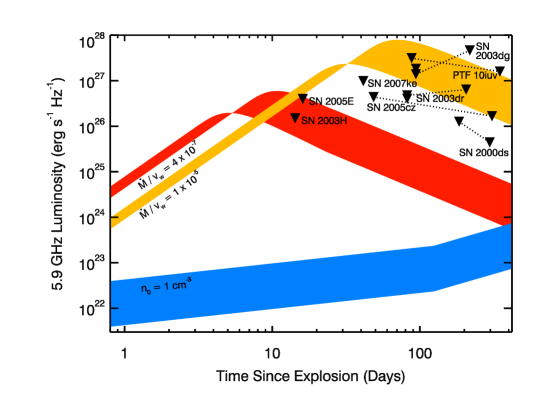
Figure 11.— 5.9 GHz upper limits for the eight Ca-rich SNe in our sample (downward facing black triangles), compared with models for a thermonuclear SN interacting with CSM, assuming explosion parameters appropriate to Ca-rich explosions ($M_{\rm ej,Ch}=0.2$ and $E_{\rm K,51}=0.4$). Observations that were carried out at frequencies differing from 5.9 GHz were normalized to 5.9 GHz assuming an optically-thin synchrotron spectral index, $\alpha=-1$. SNe with observations at more than one epoch have their limits connected by black dotted lines. The red model light curve is for a wind-stratified CSM with $\dot{M}/v_{w}=4\times 10^{-7}~{}{{{\rm M}_{\odot}\ {\rm yr}^{-1}}\over{{\rm 100\ km\ s}^{-1}}}$ (the average value for Galactic symbiotics). The orange model light curve corresponds to $\dot{M}/v_{w}=1\times 10^{-5}~{}{{{\rm M}_{\odot}\ {\rm yr}^{-1}}\over{{\rm 100\ km\ s}^{-1}}}$ (as might be expected for tidal tails from a disrupted white dwarf). The blue light curve is for uniform density surroundings with $n_{0}=1$ cm^-3. Each model light curve is actually a band of finite width, illustrating the spread in light curves produced by $\epsilon_{B}$ values ranging $0.01-0.1$; $\epsilon_{e}=0.1$ is always assumed.

6.3. Cosmologically useful SNe Ia: Broad-line, Core-normal, and Shallow-Silicon

It is the core-normal, broad-line, and shallow-silicon SNe Ia which are most often exploited as standardizeable candles, and which are well described by $M_{\rm ej,Ch}=1$ and $E_{\rm K,51}=1$. If we perform a similar statistical analysis as that described in §5.2 on the 51 SNe belonging to these sub-types, we find that, for $\epsilon_{B}=0.1$, the maximum fraction of symbiotic progenitors allowable by our radio limits is $f=0.10$ at significance $p=0.05$, or $f=0.15$ for $p=0.01$. The corresponding $p=0.05$ and $p=0.01$ values for $\epsilon_{B}=0.01$ are respectively $f=0.14$ and 0.21.

We therefore arrive at a similar conclusion as searches for early-time excesses in optical light curves of thermonuclear SNe, but using a completely independent technique. From limits on early-time excesses in $\sim$100 optical light curves, Bianco et al. (2011) find that Roche-lobe-filling red giants must comprise $<$20% of SN Ia companions, at 3$\sigma$ significance. We note that our radio limits apply to red giant + white dwarf binaries with much larger separations than the Roche-lobe-filling binary assumed in the models of Kasen (2010). Our constraints on symbiotic progenitors apply to wind-fed or wind-Roche-lobe-overflow systems (Mohamed & Podsiadlowski, 2007; Mikołajewska, 2012), being modeled on the observed Galactic population of symbiotic binaries.

There have been claims in the literature that there are differences in CSM between broad-line and core-normal SNe Ia, with broad-line SNe Ia more likely to display blueshifted Na I D absorption (Foley et al., 2012a; Maguire et al., 2013). Our radio non-detections of SNe Ia of both sub-types do not support, but can not disprove, this claim.

6.4. Super-Chandrasekhar SNe Ia

We note that an ejecta mass of $M_{\rm ej,Ch}\approx 1.4$ ($\sim$2 M_⊙) is likely more appropriate for super-Chandrasekhar explosions, while $E_{\rm K,51}\approx 1$ remains applicable (Scalzo et al., 2010, 2012; Taubenberger et al., 2011). This tweak to the model would serve to make the limits on CSM density less constraining by a factor of $1.2-2.0$ for SN 2009dc and SN 2012cu (compared with constraints listed in Tables 2 and 3).

6.5. SNe Ia-CSM

The strong H$\alpha$ emission lines displayed by SNe Ia-CSM are evidence of dense CSM, and yet no SN Ia-CSM has ever been detected at radio wavelengths (out of six observed; Table 1). Some of this apparent contradiction can be resolved by the fact that SNe Ia-CSM are rare, and therefore tend to be discovered at large distances; the nearest SN Ia-CSM in our sample is SN 2008J at 65 Mpc, and the other four are at 100–300 Mpc. Therefore, the limits on radio luminosity are less deep, compared to more normal SNe Ia.

Silverman et al. (2013) show that the optical light curve rise times of SNe Ia-CSM are longer than for normal SNe Ia, and attribute this to interaction with optically thick CSM. From the rise times, they estimate $\dot{M}/v_{w}\approx$ few $\times 10^{-1}~{}{{{\rm M}_{\odot}\ {\rm yr}^{-1}}\over{{\rm 100\ km\ s}^{-1}}}$ (see also Ofek et al. 2013). Such dense CSM would lead to the rapid deceleration of the SN ejecta; the models of outer ejecta presented in Section 4 would only apply during the first minutes following explosion, and the SN blast would enter the Sedov-Taylor phase in a matter of years. In addition, substantial free-free absorption would likely dampen the radio signature in the first year, as observed in SNe Type IIn (Chandra et al., 2012, 2015). A more complete treatment of the evolving blast wave in such dense CSM is required to assess whether radio limits constrain $\dot{M}/v_{w}\approx$ few $\times 10^{-1}~{}{{{\rm M}_{\odot}\ {\rm yr}^{-1}}\over{{\rm 100\ km\ s}^{-1}}}$, but it is outside the scope of this paper. For now, we simply note that the radio limits on SNe Ia-CSM presented here are similar to both measurements and upper limits for SNe Type IIn, which are estimated to have $\dot{M}/v_{w}\approx 10^{-3}-10^{-1}~{}{{{\rm M}_{\odot}\ {\rm yr}^{-1}}\over{{\rm 100\ km\ s}^{-1}}}$ (van Dyk et al., 1996; Williams et al., 2002; Pooley et al., 2002; Chandra et al., 2012, 2015; Fox et al., 2013).

6.6. iPTF 14atg

The SN 2002es-like event iPTF 14atg showed evidence for a non-degenerate companion star, based on observations of its early ultraviolet light curve (Cao et al., 2015). Cao et al. (2015) estimate that the companion star is located 60–90 R_⊙ from the explosion site, a separation most consistent with a massive main-sequence or sub-giant companion star. The mass loss rates from such systems would be expected to be significantly lower than for symbiotics, and it is therefore not surprising that iPTF 14atg went undetected in the radio.

We note that for this explosion, our default assumptions of $M_{\rm ej,Ch}\approx 1$ and $E_{\rm K,51}\approx 1$ are appropriate, given a measured rise time, $t_{\rm rise}=18.8$ days, expansion velocity of 10,000 km s^-1 (Cao et al., 2015), and Equations 2 and 3 of Ganeshalingam et al. (2012, see also ). Therefore the limits on $\dot{M}/v_{w}$ and $n_{0}$ given in Table 4 appropriately constrain the CSM in this system.

6.7. SN 2006X

SN 2006X was the first SN Ia observed to show time-variable Na I D absorption features (Patat et al., 2007), and remains one of a relatively small group in which this phenomenon has been detected ($\sim$3 SNe Ia; Sternberg et al. 2014). These absorption features have been interpreted as shells of CSM which are ionized by the SN radiation and then recombine. Estimates of the ionizing flux from SNe Ia imply the absorbing CSM shells are at radius, $\sim 10^{16}-10^{17}$ cm (Patat et al. 2007; see also Simon et al. 2009). The observed recombination time implies a large electron density in the shells, $\sim 10^{5}$ cm^-3

Two of the Na I D components in SN 2006X, labeled C and D by Patat et al. (2007), were observed to increase in depth between 15 days and 31 days after explosion, but had weakened again when next observed 78 days after explosion. The interpretation of these variations offered by Patat et al. is that the SN blast plowed over and ionized these components sometime between 31–78 days after explosion.

This scenario is consistent with our first two epochs of non-detections, observed 6 and 18 days after explosion, as long as the inter-shell material (at radii smaller than shells C and D) is $\lesssim$ few hundred cm^-3. However, it is outside the scope of the model presented in this paper to asses whether the third epoch, observed 287–290 days after explosion, is consistent with the SN interaction with a dense shell some $\sim$8 months previous. We look to future work to build off dynamical studies like Chevalier & Liang (1989) to predict the radio luminosity and duration from SN–shell interactions.

6.8. SN 2011fe

SN 2011fe is a remarkably nearby SN Ia and the subject of an impressive number of multi-wavelength tests to constrain the progenitor system. All came up empty handed (see Chomiuk 2013 for an early review, and further developments by Lundqvist et al. 2015, Graham et al. 2015a, and Taubenberger et al. 2015). More details on the implications of our radio limits for the progenitor system can be read in Chomiuk et al. (2012b).

6.9. SN 2012cg

SN 2012cg is a core-normal SN Ia at $\sim$15 Mpc, discovered promptly after explosion (Silverman et al., 2012; Munari et al., 2013). Marion et al. (2015) present early-time photometry that shows a blue early-time excess in the optical light curve, consistent with models for SN interaction with a non-degenerate companion (Kasen, 2010). They show that this excess is best fit with a $>$6 M_⊙ main sequence or red giant companion.

After SN 2011fe and SN 2014J, our deepest radio limits are for SN 2012cg, implying $\dot{M}/v_{w}<5\times 10^{-9}~{}{{{\rm M}_{\odot}\ {\rm yr}^{-1}}\over{{\rm 100\ km\ s}^{-1}}}$ for $\epsilon_{B}=0.1$, or $\dot{M}/v_{w}<3\times 10^{-8}~{}{{{\rm M}_{\odot}\ {\rm yr}^{-1}}\over{{\rm 100\ km\ s}^{-1}}}$ for $\epsilon_{B}=0.01$. Such low-density CSM is inconsistent with observations of symbiotics (Figure 9). Most but not all isolated red giants can also be excluded ($\dot{M}$ can extend down to $\sim$ few $\times 10^{-10}$ M_⊙ yr^-1 in relatively low-metallicity and unevolved giants; Dupree et al. 2009; Cranmer & Saar 2011). Models of main-sequence B stars with $\gtrsim$6 M_⊙ estimate $\dot{M}=10^{-11}-10^{-9}$ M_⊙ yr^-1 and $v_{w}$ = few thousand km s^-1 (Krtička, 2014), which would not be detected by our radio observations. If the mass transfer from the companion to the white dwarf is at all non-conservative (the Kasen models assume the companion is filling its Roche lobe), the CSM around the SN Ia could be significantly denser than predicted by the companion $\dot{M}/v_{w}$ alone (see discussion in Chomiuk et al. 2012b). Therefore, our radio observations of SN 2012cg can constrain but can not completely rule out the non-degenerate companion claimed by Marion et al. (2015).

6.10. SN 2014J

SN 2014J is the nearest SN Ia in decades, and our radio non-detections add to an impressive array of strong constraints on the progenitor system (Kelly et al., 2014; Margutti et al., 2014; Nielsen et al., 2014; Pérez-Torres et al., 2014; Lundqvist et al., 2015). SN 2014J is located in a region of high extinction and complex interstellar medium, and several studies do present evidence for material in the vicinity of the system, likely at $\sim 10^{19}$ cm (Foley et al., 2014b; Graham et al., 2015b; Crotts, 2015), but it remains unclear if such material is associated with the SN progenitor (Soker, 2015).

Our radio limits confirm and expand the radio non-detections of Pérez-Torres et al. (2014), who utilize the first epoch of VLA non-detections (2014 Jan 23.2) along with additional limits from eMERLIN and EVN obtained 2–5 weeks after outburst. As the earliest epoch is most constraining on a wind CSM profile, we reach very similar limits on $\dot{M}/v_{w}$ for SN 2014J. The later observations presented here (3–5 months after explosion) further constrain the presence of CSM at larger radius, $\sim$ several $\times 10^{16}$ cm.

As M82 is a starburst galaxy and SN 2014J is located at the edge of its inner CO molecular disk (Walter et al., 2002), our limits on a uniform density medium around SN 2014J, $\lesssim 3$ cm^-3, are plausibly sensitive to the interstellar medium itself. Later time observations will place even deeper constraints on a uniform interstellar medium-like component surrounding SN 2014J, and can test if the SN exploded in a wind-blown cavity (e.g., Badenes et al. 2007).

7. Conclusions

• We present observations of 85 thermonuclear SNe observed with the VLA in the first year following explosion; all yield radio non-detections.

• This is the most comprehensive study to date of radio emission from thermonuclear SNe. We worked to be complete in collecting VLA observations of thermonuclear SNe, within the parameters described in §2. These observations are a combination of new data from the Jansky VLA, unpublished archival data, and published limits.

• Our models for the radio emission from thermonuclear SNe extend lessons learned from SNe Ib/c to self-consistently predict synchrotron light curves for exploding white dwarf stars. We present models for thermonuclear SN evolution in both wind-stratified and uniform-density material.

• We present deep radio limits for SN 2012cg, with six epochs spanning 5–216 days after explosion, yielding $\dot{M}/v_{w}\lesssim 5\times 10^{-9}~{}{{{\rm M}_{\odot}\ {\rm yr}^{-1}}\over{{\rm 100\ km\ s}^{-1}}}$ for $\epsilon_{B}=0.1$. These radio observations are only rivaled by the nearby SN 2011fe and SN 2014J.

• Our sample of thermonuclear SNe spans a range of nine sub-types, including sub-luminous SNe Iax and over-luminous SNe Ia-CSM. In §6, we consider appropriate assumptions about ejecta mass and explosion energy for the various sub-types, and modify our model for radio light curves accordingly.

• The collective radio non-detections imply a scarcity of symbiotic progenitors (i.e., giant companions). We find that $<$10% of thermonuclear SNe have symbiotic progenitors if we assume $\epsilon_{B}=0.1$, or $<$16% for $\epsilon_{B}=0.01$.

In the future, this work can be improved by (a) further observations of Galactic symbiotic binaries, to further pin down their CSM properties; and (b) additional observations of a large number of SNe Ia with the VLA promptly after explosion, to significantly grow the sample of radio-observed thermonuclear SNe, allowing even stronger constraints on the fraction with red giant companion; and (c) additional radio observations of nearby thermonuclear SNe belonging to sub-types that still have relatively few radio observations (SNe Iax, SN 2002es-like, super-Chandrasekhar, and Ia-CSM explosions). Further constraints on the CSM and progenitors of SNe Ia can be provided by radio observations at longer times after explosion (1–100 years)—work that our team will present in an upcoming paper.

Table 1 Parameters for Thermonuclear SNe Observed by the VLA

SN Name	Date of Optical Max	SN Postion	Host Galaxy	Host Type	Distance	SN Ref.
		(J2000.0)			(Mpc)
Iax:
SN 2005hk	2005 Nov 11	00:27:50.87, $-$01:11:52.5	UGC 272	SAB(s)d	60	1
SN 2008A	2008 Jan 16	01:38:17.38, +35:22:13.7	NGC 634	Sa	68	2
SN 2008ha	2008 Nov 13	23:34:52.69, +18:13:35.4	UGC 12682	Irr	20	3
SN 2012Z	2012 Feb 10	03:22:05.35, $-$15:23:15.6	NGC 1309	SA(s)bc	29	4
02es-like:
iPTF 14atg	2014 May 22	12:52:44.8, +26:28:13	IC 831	E	88	5
Ca-Rich:
SN 2000ds	2000 May 10	09:11:36.24, +60:01:42.2	NGC 2768	S0	19	6
SN 2003H	2003 Jan 12	06:16:25.68, $-$21:22:23.8	NGC 2207	SAB(rs)bc pec	27	7
SN 2003dg	2003 Apr 10	11:57:31.97, $-$01:15:13.6	UGC 6934	SA(r)cd	84	7,8
SN 2003dr	2003 Apr 22	14:38:11.13, +46:38:03.4	NGC 5714	Sc	41	7,9
SN 2005E	2005 Jan 17	02:39:14.34, +01:05:55.0	NGC 1032	S0/a	37	10
SN 2005cz	2005 Jul 2	12:37:27.85, +74:11:24.5	NGC 4589	E2	29	11
SN 2007ke	2007 Sep 25	02:54:23.90, +41:34:16.3	NGC 1129	E	73	12
PTF 10iuv	2010 Jun 10	17:16:54.27, +31:33:51.7	CGCG 170-011	E0	98	12
Cool:
SN  1986G	1986 May 11	13:25:36.51, $-$43:01:54.2	NGC 5128	S0 pec	3.8	13
SN 1991bg	1991 Dec 13	12:25:03.71, +12:52:15.8	NGC 4374	E1	17	14
SN  1999by	1999 May 10	09:21:52.07, +51:00:06.6	NGC 2841	SA(r)b	18	15
SN 2002cv	2002 May 17	10 18 03.68 +21 50 06.0	NGC 3190	SA(s)a pec	25	15,16
SN 2003aa	2003 Feb 11	10:46:36.82, +13:45:32.2	NGC 3367	SB(rs)c	44	17
SN 2005ke	2005 Nov 23	03:35:04.35, $-$24:56:38.8	NGC 1371	SAB(rs)a	24	18
SN 2006bk	2006 Apr 1	15:04:33.61, +35:57:51.1	MCG +06-33-20	E	87	19
SN 2007on	2007 Nov 14	03:38:50.9, $-$35:34:30	NGC 1404	E1	19	20
SN 2011eh	2011 Jul 31	11:18:31.70, +57:58:37.2	NGC 3613	E6	29	21
SN 2011ek	2011 Aug 15	02:25:48.89, +18:32:00.0	NGC 918	SAB(rs)c	18	22
SN 2011iv	2011 Dec 11	03:38:51.35, $-$35:35:32.0	NGC 1404	E1	19	23
Broad-line:
SN 1980N	1980 Dec 12	03:22:59.8, $-$37:12:48	NGC 1316	SAB(s)0 pec	20	24
SN 1981B	1981 Mar 8	12:34:29:57, +02:11:59.3	NGC 4536	SAB(rs)bc	15	25
SN 1983G	1983 Apr 5	12:52:20.95, $-$01:12:12.3	NGC 4753	I0	18	26
SN 1984A	1984 Jan 16	12:26:55.75, +15:03:18.0	NGC 4419	SB(s)a	18	27
SN 1987N	1987 Dec 19	23:19:03.42, $-$08:28:37.7	NGC 7606	SA(s)b	33	28
SN 1989B	1989 Feb 7	11:20:13.93, +13:00:19.3	NGC 3627	SAB(s)b	10	29
SN 1992A	1992 Jan 19	03:36:27.43, $-$34:57:31.5	NGC 1380	SA0	18	30
SN 1995al	1995 Nov 8	09:50:55.97, +33:33:09.4	NGC 3021	SA(rs)bc	27	31
SN 1999cl	1999 Jun 12	12:31:56.01, +14:25:35.3	NGC 4501	SA(rs)b	19	32
SN 1999gh	1999 Dec 5	09:44:19.75, $-$21:16:25.0	NGC 2986	E2	33	33
SN 2002bo	2002 Mar 24	10 18 06.51 +21 49 41.7	NGC 3190	SA(s)a pec	25	34
SN 2005W	2005 Feb 11	01:50:45.75, +21:45:35.6	NGC 691	SA(rs)bc	37	17
SN 2006X	2006 Feb 20	12:22:53.99, +15:48:33.1	NGC 4321	SAB(s)bc	17	35
SN 2006bb	2006 Apr 1	08:33:31.09, +41:31:04.1	UGC 4468	S0	96	36
SN 2010ev	2010 Jul 7	10:25:28.99, $-$39:49:51.2	NGC 3244	SA(rs)cd	30	37
SN 2010ko	2010 Dec 12	05:32:49.44, $-$14:05:45.9	NGC 1954	SA(rs)bc	49	38
SN 2011iy	2011 Dec 3	13:08:58.39, $-$15:31:04.1	NGC 4984	(R)SAB(rs)0	21	39
SN 2012fr	2012 Nov 12	03:33:35.99, $-$36:07:37.7	NGC 1365	SB(s)b	18	40
Core-normal:
SN 1985A	1985 Jan 4	09:13:42.40, +76:28:23.9	NGC 2748	SAbc	21	41
SN 1985B	1985 Jan 6	12:02:44.08, +01:58:45.5	NGC 4045	SAB(r)a	31	41
SN  1986A	1986 Jan 30	10:46:36.60, +13:45:01.1	NGC 3367	SB(rs)c	44	42
SN  1986O	1986 Dec 20	06:25:58.0, $-$22:00:42	NGC 2227	SB(rs)c	32	43
SN 1987D	1987 Apr 18	12:19:41.11, +02:04:26.8	UGC 7370	SBbc pec	29	44
SN 1989M	1989 Jul 2	12:37:40.75, +11:49:26.1	M 58	SAB(rs)b	20	45
SN 1990M	1990 Jun 7	14:11:29.3, $-$05:02:36	NGC 5493	S0 pec	20	46
SN 1994D	1994 Mar 20	12:34:02.45, +07:42:04.7	NGC 4526	SAB(s)0	15	47
SN 1996X	1996 Apr 18	13:18:01.13, $-$26:50:45.3	NGC 5061	E0	25	31
SN 1998aq	1998 Apr 29	11:56:26.00, +55:07:38.8	NGC 3982	SAB(r)b	22	48
SN 1998bu	1998 May 19	10:46:46.03, +11:50:07.1	M 96	SAB(rs)ab	11	49
SN 2000E	2000 Feb 6	20:37:13.77, +66:05:50.2	NGC 6951	SAB(rs)bc	23	50
SN 2001bf	2001 May 16	18:01:33.99, +26:15:02.3	MCG +04-42-22	?	59	34
SN 2003cg	2003 Mar 31	10:14:15.97, +03:28:02.5	NGC 3169	SA(s)a pec	26	51
SN 2003du	2003 May 7	14:34:35.80, +59:20:03.8	UGC 9391	SBdm	35	34
SN  2003hv	2003 Sep 10	03:04:09.32, $-$26:05:07.5	NGC 1201	SA(r)0	19	34
SN  2003if	2003 Sep 1	03:19:52.61, $-$26:03:50.5	NGC 1302	(R)SB(r)0/a	20	52
SN 2007sr	2007 Dec 14	12:01:52.80, $-$18:58:21.7	NGC 4038	SB(s)m pec	21	34
PTF 10icb	2010 Jun 14	12:54:49.22, +58:52:54.8	PGC 43983	?	49	53
SN 2010fz	2010 Jul 21	09:42:04.77, +00:19:51.0	NGC 2967	SA(s)c	31	54
SN 2010ih	2010 Sep 12	07:02:43.63, $-$28:37:25.2	NGC 2325	E4	22	55
SN 2010lq	2011 Jan 6	08:32:40.98, $-$24:02:45.6	ESO 495-16	S0-a	106	56
SN 2011B	2011 Jan 10	08:55:48.50, +78:13:02.7	NGC 2655	SAB(s)0/a	24	57
SN 2011ae	2011 Feb 27	11:54:49.25, $-$16:51:43.6	PGC3̇7373	SAB(s)cd	28	58
SN 2011at	2011 Mar 15	09:28:57.56, $-$14:48:20.6	PGC 26905	SB(s)d	25	59
SN 2011by	2011 May 10	11:55:45.56, +55:19:33.8	NGC 3972	SA(s)bc	20	21
SN 2011dm	2011 Jun 27	21:56:41.59, +73:17:48.9	UGC 11861	SABdm	20	60
SN 2011fe	2011 Sep 11	14:03:05.81, +54:16:25.4	M 101	SAB(rs)cd	6.4	61
SN 2012cg	2012 Jun 2	12:27:12.83, +09:25:13.2	NGC 4424	SB(s)a	15	62
SN 2012ei	2012 Aug 27	14:24:05.71, +33:02:56.5	NGC 5611	S0	25	63
SN 2012ht	2013 Jan 4	10:53:22.75, +16:46:34.9	NGC 3447	Pec	20	64
SN 2013E	2013 Jan 14	10:00:05.52, $-$34:14:01.3	IC 2532	SB(rs)0/a	32	65
SN 2014J	2014 Feb 4	09:55:42.14, +69:40:26.0	M 82	Irr	3.4	66
Shallow-Silicon:
SN 19991T	1991 Apr 26	12:34:10.21, +02:39:56.6	NGC 4527	SAB(s)bc	14	67
Super-Mej,Ch:
SN 2009dc	2009 Apr 26	15:51:12.12, +25:42:28.0	UGC 10064	S0	89	68
PTF 10guz	2010 May 6	12:49:22.81, $-$06:23:51.3	Anonymous	?	740	69
SN 2012cu	2012 Jun 27	12:53:29.35, +02:09:39.0	NGC 4772	SA(s)a	29	70
Ia-CSM:
SN 1999E	1999 Jan 1	13:17:16.37, $-$18:33:13.4	GSC 6116 00964	Starburst	104	71
SN 2002ic	2002 Nov 27	01:30:02.55, +21:53:06.9	NEAT J013002.81+215306.9	?	273	72
SN 2005gj	2005 Oct 14	03:01:11.95, $-$00:33:13.9	SDSS J030111.99$-$003313.5	?	246	72
SN 2008J	2008 Feb 3	02:34:24.20, $-$10:50:38.5	MCG $-$02-7-33	SBbc	65	72
SN 2008cg	2008 Apr 29	15:54:15.15, +10:58:25.0	FGC 1965	Scd	121	72
PTF 11kx	2011 Jan 29	08:09:12.8, +46:18:48.8	SDSS J080913.18+461842.9	Scd	192	73

Table 2 Observations of Thermonuclear SNe with the Upgraded VLA

SN Name	Observation	VLA	Central	Band-	Flux	Time Since	Luminosity	$\dot{M}/v_{w}$	$n_{0}$
	Date	Config.	Freq.	width	Density	Explosion	Upper Limit	Upper Limit	Upper Limit
	(UT)		(GHz)	(MHz)	($\mu$Jy)	(Days)	($10^{25}$ erg s-1 Hz-1)	$\left({{{\rm M}_{\odot}\,{\rm yr}^{-1}}\over{100\ {\rm km\,s}^{-1}}}\right)$	(cm-3)
PTF 10guz	2010 May 11.1	D	4.9	256	$-16\pm 23$	29.1	4521.83	N/A	N/A
PTF 10icb	2010 Jun 4.0	D	4.9	256	$164\pm 71$	8.0	108.33	N/A	N/A
$\cdots$	2010 Jun 6.0	D	7.9	128	$7\pm 27$	10.0	25.29	$3.2\times 10^{-7}$	2500
$\cdots$	2010 Jun 8.1	D	8.4	256	$35\pm 22$	12.1	29.02	$4.0\times 10^{-7}$	2500
$\cdots$	2010 Jun 11.1	D	7.9	128	$32\pm 26$	15.1	31.60	$5.0\times 10^{-7}$	2500
SN 2010ev	2010 Jul 3.9	D	5.0	1024	$29\pm 30$	13.5	12.82	$1.6\times 10^{-7}$	1000
SN 2010fz	2010 Jul 11.9	D	6.0	2048	$-13\pm 9$	8.9	3.11	$5.0\times 10^{-8}$	400
SN 2010ih	2010 Oct 15.5	D	5.9	2048	$-18\pm 13$	51.5	2.26	$2.0\times 10^{-7}$	100
SN 2010ko	2010 Dec 9.3	C	5.9	2048	$-11\pm 6$	13.9	5.17	$1.0\times 10^{-7}$	500
SN 2010lq	2011 Jan 21.3	CnB	4.9	256	$7\pm 17$	33.3	77.99	$1.3\times 10^{-6}$	2000
SN 2011B	2011 Jan 21.1	CnB	5.9	2048	$2\pm 9$	29.1	1.99	$1.3\times 10^{-7}$	130
SN 2011ae	2011 Mar 11.3	B	5.9	2048	$-5\pm 5$	30.3	1.41	$1.0\times 10^{-7}$	100
SN 2011at	2011 Mar 17.2	B	5.9	2048	$-1\pm 5$	20.2	1.12	$5.0\times 10^{-8}$	100
SN 2011by	2011 Apr 28.0	B	5.9	2048	$16\pm 6$	6.0	1.63	$2.0\times 10^{-8}$	250
$\cdots$	2011 Apr 30.1	B	5.9	2048	$1\pm 3$	8.1	0.48	$1.0\times 10^{-8}$	63
$\cdots$	2011 Jun 10.1	A	5.9	2048	$11\pm 7$	49.1	1.53	$1.6\times 10^{-7}$	79
SN 2011dm	2011 Jun 23.1	A	5.9	2048	$-4\pm 5$	14.1	0.72	$2.5\times 10^{-8}$	79
SN 2011eh	2011 Aug 4.5	A	5.9	2048	$-3\pm 7$	17.5	2.11	$7.9\times 10^{-8}$	200
SN 2011ek	2011 Aug 9.4	A	5.9	2048	$0\pm 5$	7.4	0.58	$2.0\times 10^{-8}$	79
SN 2011fe	2011 Aug 25.8	A	5.9	2048	$8\pm 6$	1.8	0.12	$7.9\times 10^{-10}$	32
$\cdots$	2011 Aug 27.7	A	5.9	2048	$0\pm 6$	3.7	0.09	$1.3\times 10^{-9}$	20
$\cdots$	2011 Aug 30.0	A	5.9	2048	$-8\pm 7$	6.0	0.10	$2.5\times 10^{-9}$	20
$\cdots$	2011 Sept 2.7	A	5.9	2048	$1\pm 4$	9.7	0.07	$3.2\times 10^{-9}$	10
$\cdots$	2011 Sept 8.0	A	5.9	2048	$-3\pm 7$	15.0	0.10	$6.3\times 10^{-9}$	13
$\cdots$	2011 Sept 12.9	A	5.9	2048	$1\pm 6$	19.9	0.09	$1.0\times 10^{-8}$	13
SN 2011iv	2011 Dec 4.2	D	6.8	1024	$18\pm 18$	6.2	3.11	$3.2\times 10^{-8}$	500
SN 2011iy	2011 Dec 20.5	C	7.3	1024	$-39\pm 45$	34.1	7.12	$4.0\times 10^{-7}$	400
SN 2012Z	2012 Feb 2.0	C	5.9	2048	$-15\pm 6$	7.0	1.81	$2.5\times 10^{-8}$	250
SN 2012cg	2012 May 19.1	CnB	4.1	2048	$-14\pm 5$	5	0.40	$5.0\times 10^{-9}$	63
$\cdots$	2012 Jun 27.1	B	5.9	2048	$-5\pm 5$	43.1	0.40	$6.3\times 10^{-8}$	32
$\cdots$	2012 Jul 19.0	B	5.9	2048	$-12\pm 7$	65.0	0.58	$1.3\times 10^{-7}$	32
$\cdots$	2012 Aug 26.0	B	5.9	2048	$-16\pm 6$	103.0	0.48	$1.6\times 10^{-7}$	20
$\cdots$	2012 Oct 21.8	A	5.9	2048	$-1\pm 5$	159.8	0.40	$2.0\times 10^{-7}$	13
$\cdots$	2012 Dec 16.6	A	5.9	2048	$-13\pm 5$	215.6	0.40	$2.5\times 10^{-7}$	10
SN 2012cu	2012 Jun 18.2	B	5.9	2048	$1\pm 5$	15.2	1.61	$5.0\times 10^{-8}$	160
SN 2012ei	2012 Aug 25.0	B	5.9	2048	$-2\pm 6$	16.0	1.35	$5.0\times 10^{-8}$	130
SN 2012fr	2012 Oct 30.3	A	5.9	2048	$8\pm 7$	3.9	1.12	$7.9\times 10^{-9}$	200
SN 2012ht	2012 Dec 21.6	A	5.9	2048	$4\pm 5$	4.6	0.91	$7.9\times 10^{-9}$	160
$\cdots$	2013 Jan 4.5	A	5.9	2048	$0\pm 5$	18.5	0.72	$3.2\times 10^{-8}$	80
SN 2013E	2013 Jan 8.4	A$\rightarrow$D	5.9	2048	$-7\pm 8$	12.4	2.94	$6.3\times 10^{-8}$	320
SN 2014J	2014 Jan 23.2	B$\rightarrow$BnA	5.5	2048	$-12\pm 8$	6.2	0.03	$1.0\times 10^{-9}$	6.3
$\cdots$	2014 Apr 11.2	A	5.9	2048	$0\pm 7$	84.2	0.03	$2.0\times 10^{-8}$	2.5
$\cdots$	2014 Jun 12.0	A$\rightarrow$D	7.4	1024	$11\pm 10$	146.0	0.06	$6.3\times 10^{-8}$	3.2

Table 3 Archival Observations of Thermonuclear SNe with the Pre-Upgrade VLA

SN Name	Observation	VLA	Central	Program	Flux	Time Since	Luminosity	$\dot{M}$/vw	$n_{0}$
	Date	Config.	Freq.	ID	Density	Explosion	Upper Limit	Upper Limit	Upper Limit
	(UT)		(GHz)		($\mu$Jy)	(Days)	($10^{25}$ erg s-1 Hz-1)	$\left({{{\rm M}_{\odot}\,{\rm yr}^{-1}}\over{100\ {\rm km\,s}^{-1}}}\right)$	(cm-3)
SN 1998aq	1998 Jun 27.7	BnA	4.9	AL446	$56\pm 71$	77.7	15.58	$1.0\times 10^{-6}$	250
SN 1999E	1999 Jan 22.3	C	8.4	ACTST	$145\pm 80$	51.3	498.34	$7.9\times 10^{-6}$	10,000
$\cdots$	1999 Jan 22.3	C	14.9	ACTST	$439\pm 319$	51.3	1806.98	$3.2\times 10^{-5}$	40,000
$\cdots$	1999 Feb 8.4	DnC	8.4	AS568	$50\pm 46$	68.4	243.35	$6.3\times 10^{-6}$	4000
$\cdots$	1999 Feb 8.4	DnC	14.9	AS568	$140\pm 172$	68.4	849.13	$2.0\times 10^{-5}$	16,000
$\cdots$	1999 Feb 8.4	DnC	22.4	AS568	$-295\pm 281$	68.4	1091.18	$2.5\times 10^{-5}$	25,000
$\cdots$	1999 Feb 27.3	DnC	8.4	AS568	$23\pm 50$	87.3	223.93	$7.9\times 10^{-6}$	3200
$\cdots$	1999 Feb 27.3	DnC	14.9	AS568	$-226\pm 169$	87.3	656.26	$2.0\times 10^{-5}$	10,000
$\cdots$	1999 Feb 27.3	DnC	22.4	AS568	$-169\pm 175$	87.3	679.56	$2.5\times 10^{-5}$	16,000
$\cdots$	1999 Oct 28.8	BnA	8.4	AS568	$-36\pm 47$	330.8	182.51	$2.0\times 10^{-5}$	1000
SN 1999cl	1999 Oct 31.7	B	4.9	AU79	$-39\pm 61$	158.3	7.91	$1.0\times 10^{-6}$	100
SN 1999gh	2000 Mar 14.1	BnC	8.4	AJ275	$35\pm 65$	115.7	29.97	$2.5\times 10^{-6}$	500
SN 2000E	2000 Oct 8.0	D	4.9	AS568	$-21\pm 60$	263.0	11.40	$2.0\times 10^{-6}$	100
$\cdots$	2000 Oct 17.2	A	4.9	AS568	$-79\pm 44$	272.2	8.36	$1.6\times 10^{-6}$	63
SN 2000ds	2000 Oct 29.3	A	8.4	AK509	$42\pm 54$	184.3	8.81	$2.0\times 10^{-6}$	160
$\cdots$	2001 Feb 19.4	BnA	8.4	AF380	$-56\pm 24$	297.4	3.11	$1.6\times 10^{-6}$	50
SN 2001bf	2001 Jun 1.3	?	8.4	AK509	$-21\pm 49$	34.3	61.24	$1.6\times 10^{-6}$	2000
SN 2002ic	2003 Jun 16.6	A	4.9	AK550	$25\pm 33$	231.6	1105.98	$3.2\times 10^{-5}$	3200
$\cdots$	2003 Jun 17.8	A	22.4	AW608	$-202\pm 157$	232.8	4200.95	$1.5\times 10^{-4}$	32,000
SN 2003H	2003 Jan 14.3	DnC	8.4	AK509	$-27\pm 40$	14.3	10.47	$2.5\times 10^{-7}$	1000
SN 2003aa	2003 Feb 3.3	DnC	8.4	AK550	$29\pm 43$	5.3	36.61	$3.2\times 10^{-7}$	7900
$\cdots$	2003 Jun 15.0	A	8.4	AK509	$36\pm 69$	137.0	56.30	$5.0\times 10^{-6}$	790
SN 2003cg	2003 May 17–29	A	8.4	AA278	$88\pm 38$	65–77	16.34	$1.3\times 10^{-6}$	500
$\cdots$	2003 Sep 12–18	A	8.4	AA278	$-70\pm 65$	183–189	15.78	$2.5\times 10^{-6}$	250
$\cdots$	2003 Sep 21–25	BnA	8.4	AA278	$8\pm 50$	192–196	12.78	$2.5\times 10^{-6}$	200
SN 2003dg	2003 July 1.0	A	4.9	AK509	$-8\pm 66$	94.0	128.35	$5.0\times 10^{-6}$	2000
$\cdots$	2003 July 1.0	A	8.4	AK509	$8\pm 48$	94.0	167.20	$5.0\times 10^{-6}$	1600
$\cdots$	2003 Nov 1.7	B	8.4	AK573	$154\pm 77$	217.7	325.10	$2.0\times 10^{-5}$	2000
SN 2003dr	2003 July 1.0	A	4.9	AK509	$81\pm 68$	82.0	28.37	$2.0\times 10^{-6}$	630
$\cdots$	2003 July 1.0	A	8.4	AK509	$-111\pm 47$	82.0	57.33	$2.0\times 10^{-6}$	790
$\cdots$	2003 Nov 1.7	B	8.4	AK573	$28\pm 65$	205.7	44.86	$5.0\times 10^{-6}$	500
SN 2003du	2003 Oct 17.0	BnA	8.4	AS779	$-76\pm 33$	181.0	14.51	$2.5\times 10^{-6}$	200
SN 2005E	2005 Jan 21.1	BnA	8.4	AS796	$11\pm 53$	16.1	27.85	$5.0\times 10^{-7}$	2000
SN 2005W	2005 Feb 7.9	BnA	8.4	AW641	$-50\pm 52$	13.5	25.56	$4.0\times 10^{-7}$	2500
SN 2005cz	2005 Aug 7.6	C	8.4	AS846	$110\pm 65$	48.6	30.70	$1.3\times 10^{-6}$	1000
$\cdots$	2006 Apr 24.1	A	4.9	AC807	$16\pm 61$	308.1	20.03	$3.2\times 10^{-6}$	130
SN 2005gj	2005 Nov 25.4	D	8.4	AS869	$26\pm 32$	72.4	883.55	$1.6\times 10^{-5}$	10,000
$\cdots$	2005 Dec 6.1	D	8.4	AK583	$75\pm 40$	83.1	1412.23	$2.5\times 10^{-5}$	16,000
$\cdots$	2006 Jan 2.1	D	8.4	AK583	$45\pm 25$	110.1	869.07	$2.0\times 10^{-5}$	7900
$\cdots$	2006 Feb 26.9	A	1.4	AW675	$-29\pm 52$	165.9	1129.79	N/A	N/A
$\cdots$	2006 Feb 26.9	A	8.4	AW675	$-12\pm 35$	165.9	760.43	$2.5\times 10^{-5}$	5000
SN 2005hk	2006 Jan 31.0	A	8.4	AS846	$77\pm 29$	96.0	70.66	$4.0\times 10^{-6}$	1300
$\cdots$	2006 Feb 4.0	A	4.9	AS846	$19\pm 96$	100.0	132.26	$4.0\times 10^{-6}$	1300
$\cdots$	2006 Feb 4.0	A	8.4	AS846	$131\pm 90$	100.0	172.76	$6.3\times 10^{-6}$	2000
SN 2005ke	2005 Nov 18.2	D	8.4	AS846	$70\pm 59$	8.2	17.03	$2.0\times 10^{-7}$	2500
$\cdots$	2006 Jan 27.1	A	8.4	AS846	$21\pm 58$	78.1	13.44	$1.3\times 10^{-6}$	400
SN 2006X	2006 Feb 9.3	A	8.4	AS875	$-27\pm 18$	5.9	1.87	$2.5\times 10^{-8}$	400
$\cdots$	2006 Feb 9.4	A	22.4	AW682	$75\pm 58$	6.0	8.61	$1.6\times 10^{-7}$	3200
$\cdots$	2006 Feb 21.4	A	1.4	AW682	$-14\pm 54$	18.0	5.60	$6.3\times 10^{-8}$	160
$\cdots$	2006 Feb 21.4	A	8.4	AW682	$-26\pm 24$	18.0	2.49	$1.0\times 10^{-7}$	320
$\cdots$	2006 Nov 17.6	C	4.8	AC867	$-36\pm 42$	287.2	4.36	$1.3\times 10^{-6}$	40
$\cdots$	2006 Nov 20.6	C	8.4	AC867	$-19\pm 36$	290.2	3.74	$1.6\times 10^{-6}$	50
SN 2006bb	2006 Apr 3.1	A	8.4	AK583	$79\pm 58$	18.7	279.04	N/A	N/A
SN 2006bk	2006 Apr 13.4	A	8.4	AS877	$5\pm 48$	25.4	134.97	$2.0\times 10^{-6}$	5000
SN 2007ke	2007 Oct 24.4	BnA	8.4	AS887	$-32\pm 36$	41.4	68.88	$2.0\times 10^{-6}$	2000
SN 2007on	2007 Dec 7.3	B	1.4	AS935	$-95\pm 535$	36.3	69.34	N/A	N/A
$\cdots$	2007 Dec 7.2	B	8.4	AS935	$3\pm 33$	36.2	4.41	$3.2\times 10^{-7}$	250
SN 2007sr	2007 Dec 23.4	B	8.4	AS887	$33\pm 48$	27.4	9.34	$4.0\times 10^{-7}$	630
SN 2008A	2008 Jan 6.1	B	8.4	AS887	$-59\pm 46$	5.1	76.37	N/A	N/A
SN 2008J	2008 Mar 1.8	CnB	8.4	AS887	$-36\pm 49$	57.8	74.33	$2.5\times 10^{-6}$	1600
$\cdots$	2008 Sep 25.4	D	8.4	AC938	$119\pm 107$	265.4	222.47	$2.0\times 10^{-5}$	1300
$\cdots$	2008 Dec 16.2	A	8.4	AC938	$96\pm 62$	347.2	142.59	$1.6\times 10^{-5}$	790
SN 2008cg	2008 Jun 13.1	DnC	8.4	AC881	$30\pm 55$	75.1	341.67	$7.9\times 10^{-6}$	5000
$\cdots$	2008 Jul 1.2	D	8.4	AC881	$7\pm 38$	93.2	212.01	$7.9\times 10^{-6}$	2500
$\cdots$	2008 Dec 13.6	A	8.4	AC938	$60\pm 52$	258.6	378.47	$2.5\times 10^{-5}$	2000
SN 2008ha	2008 Nov 22.0	A	8.4	AS929	$-23\pm 48$	24.0	6.89	$3.2\times 10^{-7}$	500
SN 2009dc	2009 Apr 28.5	B	8.4	AS929	$24\pm 48$	26.5	159.25	$2.5\times 10^{-6}$	6300

Table 4 Published Observations of SNe Ia with the VLA

SN Name	Observation	VLA	Central	$\sigma_{\nu}$	Time Since	Luminosity	$\dot{M}$/vw	$n_{0}$
	Date	Config.	Freq.		Explosion	Upper Limit	Upper Limit	Upper Limit
	(UT)		(GHz)	(mJy)	(Days)	($10^{25}$ erg s-1 Hz-1)	$\left({{{\rm M}_{\odot}\,{\rm yr}^{-1}}\over{100\ {\rm km\,s}^{-1}}}\right)$	(cm-3)
SN 1980N	1981 Feb 3	A	4.8	0.20	70	23.37	$1.0\times 10^{-6}$	400
SN 1981B	1981 Mar 11	A	4.8	0.10	20	6.57	$1.6\times 10^{-7}$	400
$\cdots$	1981 Apr 9	A	4.8	0.13	49	8.54	$4.0\times 10^{-7}$	250
$\cdots$	1981 May 14	B	4.8	0.17	84	11.17	$7.9\times 10^{-7}$	200
$\cdots$	1981 Jun 19	B	4.8	0.20	120	13.14	$1.3\times 10^{-6}$	200
$\cdots$	1981 Aug 13	B	4.8	0.30	175	19.72	$2.0\times 10^{-6}$	200
$\cdots$	1981 Nov 11	C	4.8	0.07	265	4.60	$1.3\times 10^{-6}$	50
SN 1983G	1983 May 27	C	4.8	0.07	69	6.62	$5.0\times 10^{-7}$	160
SN 1984A	1984 Mar 5	BnC	4.8	0.10	66	9.46	$6.3\times 10^{-7}$	200
SN 1985A	1985 Feb 1	A	4.8	0.07	46	9.02	$4.0\times 10^{-7}$	250
$\cdots$	1985 Feb 8	A	1.4	0.07	53	2.63	$1.0\times 10^{-7}$	40
$\cdots$	1985 Feb 17	A	1.4	0.09	62	3.38	$1.3\times 10^{-7}$	40
$\cdots$	1985 Feb 17	A	4.8	0.07	62	9.02	$5.0\times 10^{-7}$	200
$\cdots$	1985 Mar 2	A	1.4	0.07	75	2.63	$1.3\times 10^{-7}$	32
$\cdots$	1985 Apr 5	A/B	1.4	0.08	109	3.00	$2.0\times 10^{-7}$	25
$\cdots$	1985 Oct 28	C/D	1.4	0.10	315	3.76	$6.3\times 10^{-7}$	13
SN 1985B	1985 Feb 22	A	1.4	0.17	65	13.92	$4.0\times 10^{-7}$	130
$\cdots$	1985 Feb 22	A	4.8	0.19	65	53.33	$1.6\times 10^{-6}$	790
$\cdots$	1985 Mar 18	A/B	1.4	0.40	89	32.75	$7.9\times 10^{-7}$	200
$\cdots$	1985 Mar 18	A/B	4.8	0.06	89	16.84	$1.0\times 10^{-6}$	250
$\cdots$	1985 Sep 15	C	1.4	0.08	270	6.55	$7.9\times 10^{-7}$	25
$\cdots$	1985 Sep 15	C	4.8	0.05	270	14.03	$2.5\times 10^{-6}$	100
SN 1986A	1986 Feb 7	D	4.8	0.22	26	124.41	$2.0\times 10^{-6}$	4000
$\cdots$	1986 Feb 25	A	1.4	0.36	44	59.38	N/A	N/A
$\cdots$	1986 Feb 25	A	4.8	0.12	44	67.86	$1.6\times 10^{-6}$	1300
$\cdots$	1986 Mar 16	A	4.8	0.05	63	28.27	$1.0\times 10^{-6}$	500
$\cdots$	1986 Apr 3	A	4.8	0.09	81	50.89	$2.0\times 10^{-6}$	630
$\cdots$	1986 Jun 15	A/B	1.4	0.15	154	24.74	$1.0\times 10^{-6}$	100
$\cdots$	1986 Jun 15	A/B	4.8	0.09	154	50.89	$3.2\times 10^{-6}$	400
$\cdots$	1986 Oct 16	B/C	1.4	0.25	277	41.23	$2.5\times 10^{-6}$	100
$\cdots$	1986 Oct 16	B/C	4.8	0.08	277	45.24	$5.0\times 10^{-6}$	250
SN 1986G	1986 May 14	A	4.8	1.06	16	4.47	$1.0\times 10^{-7}$	320
$\cdots$	1986 May 21	A	4.8	0.70	23	2.95	$1.0\times 10^{-7}$	200
$\cdots$	1986 May 21	A	15.0	3.21	23	42.31	$1.3\times 10^{-6}$	3200
$\cdots$	1986 Jun 8	A	4.8	1.02	41	4.30	$2.5\times 10^{-7}$	160
$\cdots$	1986 Jul 6	A/B	4.8	1.52	69	6.41	$5.0\times 10^{-7}$	160
$\cdots$	1986 Jul 6	A/B	15.0	1.32	69	17.40	$1.6\times 10^{-6}$	790
$\cdots$	1986 Sep 20	C	4.8	2.49	145	10.50	$1.3\times 10^{-6}$	130
$\cdots$	1986 Sep 20	C	15.0	1.27	145	16.74	$3.2\times 10^{-6}$	400
$\cdots$	1987 Jan 4	C	4.8	2.71	251	11.43	$2.0\times 10^{-6}$	100
$\cdots$	1987 Jan 4	C	15.0	1.38	251	18.19	$5.0\times 10^{-6}$	320
SN 1986O	1987 Feb 12	C/D	1.4	0.80	72	69.79	$1.6\times 10^{-6}$	500
$\cdots$	1987 Feb 12	C/D	4.8	0.07	72	20.94	$1.0\times 10^{-6}$	400
$\cdots$	1987 Feb 12	C/D	15.0	0.18	72	168.24	$7.9\times 10^{-6}$	4000
$\cdots$	1987 Apr 11	D	4.8	0.08	130	23.93	$2.0\times 10^{-6}$	250
$\cdots$	1987 Apr 11	D	15.0	0.16	130	149.55	$1.0\times 10^{-5}$	2500
$\cdots$	1987 May 24	D	4.8	0.08	173	23.93	$2.5\times 10^{-6}$	200
$\cdots$	1987 May 24	D	15.0	0.15	173	140.20	$1.3\times 10^{-5}$	2000
$\cdots$	1987 Aug 28	A	4.8	0.07	269	20.94	$3.2\times 10^{-6}$	160
SN 1987D	1987 May 15	D	4.8	0.20	45	49.13	$1.3\times 10^{-6}$	1000
$\cdots$	1987 Jun 4	D	4.8	0.26	65	63.87	$2.0\times 10^{-6}$	1000
$\cdots$	1987 Jun 21	A	4.8	0.06	82	14.74	$1.0\times 10^{-6}$	250
$\cdots$	1987 Sep 18	A	4.8	0.07	171	17.20	$2.0\times 10^{-6}$	160
SN 1987N	1987 Dec 20	B	1.4	0.13	18	12.06	N/A	N/A
$\cdots$	1987 Dec 20	B	4.8	0.10	18	31.81	$5.0\times 10^{-7}$	1600
$\cdots$	1988 Jan 12	B	1.4	0.10	41	9.28	$2.0\times 10^{-7}$	130
$\cdots$	1988 Jan 12	B	4.8	0.08	41	25.45	$7.9\times 10^{-7}$	630
$\cdots$	1988 Feb 1	B	1.4	0.11	61	10.21	$2.5\times 10^{-7}$	100
$\cdots$	1988 Feb 1	B	4.8	0.09	61	28.63	$1.0\times 10^{-6}$	500
$\cdots$	1988 Mar 31	C	1.4	0.23	120	21.34	$7.9\times 10^{-7}$	100
$\cdots$	1988 Mar 31	C	4.8	0.07	120	22.27	$1.6\times 10^{-6}$	250
$\cdots$	1988 Apr 11	C	1.4	0.22	131	20.41	$7.9\times 10^{-7}$	100
$\cdots$	1988 Apr 11	C	4.8	0.40	131	127.23	$5.0\times 10^{-6}$	1000
$\cdots$	1988 Aug 22	D	4.8	0.08	264	25.45	$3.2\times 10^{-6}$	160
SN 1989B	1989 Feb 2	A	4.8	0.08	12	2.34	$5.0\times 10^{-8}$	200
$\cdots$	1989 Feb 2	A	8.4	0.06	12	3.07	$7.9\times 10^{-8}$	400
$\cdots$	1989 Feb 3	A	4.8	0.03	13	0.88	$2.5\times 10^{-8}$	79
$\cdots$	1989 Feb 3	A	8.4	0.03	13	1.53	$5.0\times 10^{-8}$	250
$\cdots$	1989 Mar 6	A/B	4.8	0.06	44	1.75	$1.6\times 10^{-7}$	79
$\cdots$	1989 Mar 27	B	4.8	0.06	65	1.75	$2.0\times 10^{-7}$	63
$\cdots$	1989 Apr 6	B	4.8	0.07	75	2.04	$2.5\times 10^{-7}$	63
$\cdots$	1989 May 15	BnC	4.8	0.06	114	1.75	$3.2\times 10^{-7}$	40
SN 1989M	1989 Jul 17	C	4.8	0.13	33	15.19	$5.0\times 10^{-7}$	500
$\cdots$	1989 Sep 4	C	4.8	0.10	82	11.68	$7.9\times 10^{-7}$	200
$\cdots$	1989 Oct 24	C/C	4.8	0.07	132	8.18	$1.0\times 10^{-6}$	130
$\cdots$	1989 Dec 21	D	4.8	0.05	190	5.84	$1.0\times 10^{-6}$	63
$\cdots$	1990 Feb 13	D/A	4.8	0.08	244	9.35	$1.6\times 10^{-6}$	79
$\cdots$	1990 May 29	A	4.8	0.15	349	17.53	$3.2\times 10^{-6}$	100
SN 1990M	1990 Jun 29	A/B	8.4	0.04	40	8.18	$5.0\times 10^{-7}$	400
$\cdots$	1990 Dec 14	C	8.4	0.04	208	8.18	$2.0\times 10^{-6}$	130
SN 1991T	1991 May 8	D	8.4	0.05	30	5.01	$3.2\times 10^{-7}$	320
$\cdots$	1991 May 8	D	15.0	0.06	30	10.73	$6.3\times 10^{-7}$	1000
$\cdots$	1991 Jul 9	A	8.4	0.06	92	6.01	$7.9\times 10^{-7}$	200
$\cdots$	1991 Jul 9	A	15.0	0.20	92	35.78	$3.2\times 10^{-6}$	1000
SN 1991bg	1991 Dec 26	B	1.4	0.26	26	6.40	$1.0\times 10^{-7}$	130
$\cdots$	1991 Dec 26	B	8.4	0.16	26	23.64	$6.3\times 10^{-7}$	1300
SN 1992A	1992 Jan 27	B/C	4.8	0.03	25	2.84	$1.3\times 10^{-7}$	160
$\cdots$	1992 Oct 9	A	4.8	0.15	281	14.20	$2.5\times 10^{-6}$	100
SN 1994D	1994 May 4	A	4.8	0.06	63	3.94	$3.2\times 10^{-7}$	130
SN 1995al	1995 Nov 8	B	1.4	0.08	17	4.97	$5.0\times 10^{-8}$	130
SN 1996X	1996 May 29	DnC	8.4	0.09	59	28.75	$1.6\times 10^{-6}$	790
SN 1998bu	1998 May 13	A	8.4	0.07	12	4.33	$1.0\times 10^{-7}$	630
$\cdots$	1998 May 31	A	8.4	0.04	30	2.47	$2.0\times 10^{-7}$	200
$\cdots$	1998 May 31	A	15.0	0.18	30	19.88	$1.0\times 10^{-6}$	1600
$\cdots$	1998 Jun 9	BnA	8.4	0.05	39	3.09	$2.5\times 10^{-7}$	200
$\cdots$	1998 Jun 9	BnA	15.0	0.23	39	25.40	$1.3\times 10^{-6}$	1600
$\cdots$	1999 Jan 7	C	4.8	0.07	251	2.47	$7.9\times 10^{-7}$	32
$\cdots$	1999 Jan 7	C	8.4	0.06	251	3.71	$1.3\times 10^{-6}$	63
SN 1999by	1999 May 7	D	8.4	0.07	10	11.59	$1.6\times 10^{-7}$	1600
$\cdots$	1999 May 24	D	8.4	0.08	27	13.25	$5.0\times 10^{-7}$	790
SN 2002bo	2002 May 21	BnA	8.4	0.06	75	19.17	$1.3\times 10^{-6}$	500
$\cdots$	2002 May 21	BnA	15.0	0.28	75	159.74	$7.9\times 10^{-6}$	4000
$\cdots$	2002 May 21	BnA	22.0	0.36	75	301.21	$1.3\times 10^{-5}$	8000
$\cdots$	2002 May 21	BnA	43.0	0.62	75	1013.94	$4.0\times 10^{-5}$	40,000
$\cdots$	2002 Jun 12	B	1.4	0.06	97	3.19	$2.0\times 10^{-7}$	25
$\cdots$	2002 Jun 12	B	4.8	0.08	97	14.60	$1.0\times 10^{-6}$	250
$\cdots$	2002 Jun 12	B	8.4	0.07	97	22.36	$2.0\times 10^{-6}$	500
SN 2002cv	2002 May 21	BnA	8.4	0.06	17	19.17	$4.0\times 10^{-7}$	1600
$\cdots$	2002 May 21	BnA	15.0	0.28	17	159.74	$2.5\times 10^{-6}$	13,000
$\cdots$	2002 May 21	BnA	22.0	0.36	17	301.21	$4.0\times 10^{-6}$	25,000
$\cdots$	2002 May 21	BnA	43.0	0.62	17	1013.94	$1.3\times 10^{-5}$	100,000
$\cdots$	2002 Jun 12	B	1.4	0.06	39	3.19	$7.9\times 10^{-8}$	50
$\cdots$	2002 Jun 12	B	4.8	0.08	39	14.60	$5.0\times 10^{-7}$	400
$\cdots$	2002 Jun 12	B	8.4	0.07	39	22.36	$1.0\times 10^{-6}$	1000
SN 2003hv	2003 Oct 21	B	8.4	0.05	59	9.23	$7.9\times 10^{-7}$	320
SN 2003if	2003 Oct 21	B	8.4	0.05	68	10.22	$7.9\times 10^{-7}$	320
PTF 10iuv	2010 Aug 25.1	D	8.5	0.063	88	312.96	$1.0\times 10^{-5}$	4000
$\cdots$	2011 May 12.2	BnA	8.5	0.032	348	158.96	$2.0\times 10^{-5}$	790
PTF 11kx	2011 Mar 30.2	B	8.4	0.023	90	433.39	$1.3\times 10^{-5}$	5000
SN 2011fe	2011 Aug 25.0	A	8.5	0.025	1	0.37	$1.0\times 10^{-9}$	158
SN 2014J	2014 Jan 24.4	B$\rightarrow$BnA	22.0	0.008	7	0.03	$4.0\times 10^{-9}$	20
iPTF 14atg	2014 May 16.2	A	6.1	0.010	13	28.27	$4.0\times 10^{-7}$	2000
$\cdots$	2014 May 16.2	A	22.0	0.010	13	103.67	$1.6\times 10^{-6}$	13,000

References

- Amanullah et al. (2015) Amanullah, R., Johansson, J., Goobar, A., et al. 2015, MNRAS, 453, 3300
- Arnett (1982) Arnett, W. D. 1982, ApJ, 253, 785
- Arsenault & D’Odorico (1988) Arsenault, R., & D’Odorico, S. 1988, A&A, 202, 55
- Ashok & Banerjee (2003) Ashok, N. M., & Banerjee, D. P. K. 2003, A&A, 409, 1007
- Badenes et al. (2005) Badenes, C., Borkowski, K. J., & Bravo, E. 2005, ApJ, 624, 198
- Badenes et al. (2003) Badenes, C., Bravo, E., Borkowski, K. J., & Domínguez, I. 2003, ApJ, 593, 358
- Badenes et al. (2007) Badenes, C., Hughes, J. P., Bravo, E., & Langer, N. 2007, ApJ, 662, 472
- Badenes et al. (2008) Badenes, C., Hughes, J. P., Cassam-Chenaï, G., & Bravo, E. 2008, ApJ, 680, 1149
- Benetti et al. (2005) Benetti, S., Cappellaro, E., Mazzali, P. A., et al. 2005, ApJ, 623, 1011
- Berger et al. (2002) Berger, E., Kulkarni, S. R., & Chevalier, R. A. 2002, ApJ, 577, L5
- Berger et al. (2003) Berger, E., Soderberg, A. M., & Frail, D. A. 2003, IAU Circ., 8157, 2
- Bianco et al. (2011) Bianco, F. B., Howell, D. A., Sullivan, M., et al. 2011, ApJ, 741, 20
- Blondin et al. (2006) Blondin, S., Modjaz, M., Kirshner, R., Challis, P., & Peters, W. 2006, CBET, 488, 1
- Blondin et al. (2009) Blondin, S., Prieto, J. L., Patat, F., et al. 2009, ApJ, 693, 207
- Branch et al. (1995) Branch, D., Livio, M., Yungelson, L. R., Boffi, F. R., & Baron, E. 1995, PASP, 107, 1019
- Branch et al. (2006) Branch, D., Dang, L. C., Hall, N., et al. 2006, PASP, 118, 560
- Broersen et al. (2014) Broersen, S., Chiotellis, A., Vink, J., & Bamba, A. 2014, MNRAS, 441, 3040
- Brown et al. (2012) Brown, P. J., Dawson, K. S., Harris, D. W., et al. 2012, ApJ, 749, 18
- Buta et al. (1985) Buta, R. J., Corwin, Jr., H. G., & Opal, C. B. 1985, PASP, 97, 229
- Cao et al. (2015) Cao, Y., Kulkarni, S. R., Howell, D. A., et al. 2015, Nature, 521, 328
- Challis et al. (2010) Challis, P., Marion, G. H., Kirshner, R., et al. 2010, CBET, 2575, 1
- Chandler & Marvil (2014) Chandler, C. J., & Marvil, J. 2014, ATel, 5812, 1
- Chandra et al. (2006) Chandra, P., Chevalier, R., & Patat, F. 2006, ATel, 954, 1
- Chandra et al. (2012) Chandra, P., Chevalier, R. A., Chugai, N., et al. 2012, ApJ, 755, 110
- Chandra et al. (2015) Chandra, P., Chevalier, R. A., Chugai, N., Fransson, C., & Soderberg, A. M. 2015, ApJ, 810, 32
- Chandra & Soderberg (2008) Chandra, P., & Soderberg, A. 2008, ATel, 1594, 1
- Chevalier (1982a) Chevalier, R. A. 1982a, ApJ, 258, 790
- Chevalier (1982b) —. 1982b, ApJ, 259, 302
- Chevalier (1996) Chevalier, R. A. 1996, in ASP Conf. Ser., Vol. 93, Radio Emission from the Stars and the Sun, ed. A. R. Taylor & J. M. Paredes, 125
- Chevalier (1998) —. 1998, ApJ, 499, 810
- Chevalier & Fransson (2006) Chevalier, R. A., & Fransson, C. 2006, ApJ, 651, 381
- Chevalier & Liang (1989) Chevalier, R. A., & Liang, E. P. 1989, ApJ, 344, 332
- Childress et al. (2013) Childress, M. J., Scalzo, R. A., Sim, S. A., et al. 2013, ApJ, 770, 29
- Chomiuk (2013) Chomiuk, L. 2013, PASA, 30, 46
- Chomiuk & Soderberg (2010a) Chomiuk, L., & Soderberg, A. 2010a, ATel, 2659, 1
- Chomiuk & Soderberg (2010b) —. 2010b, ATel, 2762, 1
- Chomiuk et al. (2012a) Chomiuk, L., Soderberg, A., Simon, J., & Foley, R. 2012a, ATel, 4453, 1
- Chomiuk et al. (2014) Chomiuk, L., Zauderer, B. A., Margutti, R., & Soderberg, A. 2014, ATel, 5800, 1
- Chomiuk et al. (2012b) Chomiuk, L., Soderberg, A. M., Moe, M., et al. 2012b, ApJ, 750, 164
- Chugai (2008) Chugai, N. N. 2008, Astronomy Letters, 34, 389
- Colgate & McKee (1969) Colgate, S. A., & McKee, C. 1969, ApJ, 157, 623
- Cranmer & Saar (2011) Cranmer, S. R., & Saar, S. H. 2011, ApJ, 741, 54
- Crotts (2015) Crotts, A. P. S. 2015, ApJ, 804, L37
- Cumming et al. (1996) Cumming, R. J., Lundqvist, P., Smith, L. J., Pettini, M., & King, D. L. 1996, MNRAS, 283, 1355
- Dalcanton et al. (2009) Dalcanton, J. J., Williams, B. F., Seth, A. C., et al. 2009, ApJS, 183, 67
- Dan et al. (2011) Dan, M., Rosswog, S., Guillochon, J., & Ramirez-Ruiz, E. 2011, ApJ, 737, 89
- della Valle et al. (1996) della Valle, M., Benetti, S., & Panagia, N. 1996, ApJ, 459, L23
- Di Stefano et al. (2011) Di Stefano, R., Voss, R., & Claeys, J. S. W. 2011, ApJ, 738, L1
- Dilday et al. (2012) Dilday, B., Howell, D. A., Cenko, S. B., et al. 2012, Science, 337, 942
- Dupree et al. (2009) Dupree, A. K., Smith, G. H., & Strader, J. 2009, AJ, 138, 1485
- Dwarkadas & Chevalier (1998) Dwarkadas, V. V., & Chevalier, R. A. 1998, ApJ, 497, 807
- Elias-Rosa et al. (2006) Elias-Rosa, N., Benetti, S., Cappellaro, E., et al. 2006, MNRAS, 369, 1880
- Elias-Rosa et al. (2008) Elias-Rosa, N., Benetti, S., Turatto, M., et al. 2008, MNRAS, 384, 107
- Filippenko & Chornock (2000) Filippenko, A. V., & Chornock, R. 2000, IAU Circ., 7511, 2
- Filippenko & Chornock (2003) —. 2003, IAU Circ., 8084, 4
- Filippenko et al. (2003) Filippenko, A. V., Chornock, R., Swift, B., et al. 2003, IAU Circ., 8159, 2
- Filippenko et al. (1992) Filippenko, A. V., Richmond, M. W., Matheson, T., et al. 1992, ApJ, 384, L15
- Folatelli et al. (2010) Folatelli, G., Phillips, M. M., Burns, C. R., et al. 2010, AJ, 139, 120
- Foley et al. (2010) Foley, R. J., Brown, P. J., Rest, A., et al. 2010, ApJ, 708, L61
- Foley et al. (2014a) Foley, R. J., McCully, C., Jha, S. W., et al. 2014a, ApJ, 792, 29
- Foley et al. (2015) Foley, R. J., Van Dyk, S. D., Jha, S. W., et al. 2015, ApJ, 798, L37
- Foley et al. (2009) Foley, R. J., Chornock, R., Filippenko, A. V., et al. 2009, AJ, 138, 376
- Foley et al. (2012a) Foley, R. J., Simon, J. D., Burns, C. R., et al. 2012a, ApJ, 752, 101
- Foley et al. (2012b) Foley, R. J., Kromer, M., Howie Marion, G., et al. 2012b, ApJ, 753, L5
- Foley et al. (2012c) Foley, R. J., Challis, P. J., Filippenko, A. V., et al. 2012c, ApJ, 744, 38
- Foley et al. (2013) Foley, R. J., Challis, P. J., Chornock, R., et al. 2013, ApJ, 767, 57
- Foley et al. (2014b) Foley, R. J., Fox, O. D., McCully, C., et al. 2014b, MNRAS, 443, 2887
- Fox et al. (2013) Fox, O. D., Filippenko, A. V., Skrutskie, M. F., et al. 2013, AJ, 146, 2
- Ganeshalingam et al. (2011) Ganeshalingam, M., Li, W., & Filippenko, A. V. 2011, MNRAS, 416, 2607
- Ganeshalingam et al. (2010) Ganeshalingam, M., Li, W., Filippenko, A. V., et al. 2010, ApJS, 190, 418
- Ganeshalingam et al. (2012) —. 2012, ApJ, 751, 142
- Garnavich et al. (2004) Garnavich, P. M., Bonanos, A. Z., Krisciunas, K., et al. 2004, ApJ, 613, 1120
- Goranskij et al. (2010) Goranskij, V., Shugarov, S., Zharova, A., Kroll, P., & Barsukova, E. A. 2010, Peremennye Zvezdy, 30, 4
- Graham (1988) Graham, J. R. 1988, ApJ, 326, L51
- Graham et al. (2015a) Graham, M. L., Nugent, P. E., Sullivan, M., et al. 2015a, MNRAS, 454, 1948
- Graham et al. (2015b) Graham, M. L., Valenti, S., Fulton, B. J., et al. 2015b, ApJ, 801, 136
- Greisen (2003) Greisen, E. W. 2003, in Astrophysics and Space Science Library, Vol. 285, Information Handling in Astronomy—Historical Vistas, ed. A. Heck, 109
- Guillochon et al. (2010) Guillochon, J., Dan, M., Ramirez-Ruiz, E., & Rosswog, S. 2010, ApJ, 709, L64
- Gutiérrez et al. (2011) Gutiérrez, C., Folatelli, G., Pignata, G., Hamuy, M., & Taubenberger, S. 2011, Boletin de la Asociacion Argentina de Astronomia La Plata Argentina, 54, 109
- Hachisu et al. (1999) Hachisu, I., Kato, M., & Nomoto, K. 1999, ApJ, 522, 487
- Hamilton & Fesen (1988) Hamilton, A. J. S., & Fesen, R. A. 1988, ApJ, 327, 178
- Hamuy et al. (1991) Hamuy, M., Phillips, M. M., Maza, J., et al. 1991, AJ, 102, 208
- Hamuy et al. (2003) Hamuy, M., Phillips, M. M., Suntzeff, N. B., et al. 2003, Nature, 424, 651
- Hancock et al. (2011) Hancock, P. P., Gaensler, B. M., & Murphy, T. 2011, ApJ, 735, L35
- Harris et al. (2010) Harris, G. L. H., Rejkuba, M., & Harris, W. E. 2010, PASA, 27, 457
- Hayden et al. (2010) Hayden, B. T., Garnavich, P. M., Kasen, D., et al. 2010, ApJ, 722, 1691
- Höflich (1995) Höflich, P. 1995, ApJ, 443, 89
- Horesh et al. (2012) Horesh, A., Kulkarni, S. R., Fox, D. B., et al. 2012, ApJ, 746, 21
- Horesh et al. (2013) Horesh, A., Stockdale, C., Fox, D. B., et al. 2013, MNRAS, 436, 1258
- Howell (2011) Howell, D. A. 2011, Nature Communications, 2, 350
- Howell et al. (2006) Howell, D. A., Sullivan, M., Nugent, P. E., et al. 2006, Nature, 443, 308
- Hughes et al. (2007) Hughes, J. P., Chugai, N., Chevalier, R., Lundqvist, P., & Schlegel, E. 2007, ApJ, 670, 1260
- Iben & Tutukov (1984) Iben, Jr., I., & Tutukov, A. V. 1984, ApJS, 54, 335
- Itoh et al. (1988) Itoh, H., Masai, K., & Nomoto, K. 1988, ApJ, 334, 279
- Jeffery & Hamann (2010) Jeffery, C. S., & Hamann, W.-R. 2010, MNRAS, 404, 1698
- Jha et al. (1999) Jha, S., Garnavich, P. M., Kirshner, R. P., et al. 1999, ApJS, 125, 73
- Ji et al. (2013) Ji, S., Fisher, R. T., García-Berro, E., et al. 2013, ApJ, 773, 136
- Justham (2011) Justham, S. 2011, ApJ, 730, L34+
- Kandrashoff et al. (2011) Kandrashoff, M., Kelly, J., Cenko, S. B., et al. 2011, CBET, 2745, 1
- Kasen (2010) Kasen, D. 2010, ApJ, 708, 1025
- Kasliwal et al. (2012) Kasliwal, M. M., Kulkarni, S. R., Gal-Yam, A., et al. 2012, ApJ, 755, 161
- Kawabata et al. (2010) Kawabata, K. S., Maeda, K., Nomoto, K., et al. 2010, Nature, 465, 326
- Kelly et al. (2014) Kelly, P. L., Fox, O. D., Filippenko, A. V., et al. 2014, ApJ, 790, 3
- Kerzendorf et al. (2014) Kerzendorf, W. E., Childress, M., Scharwächter, J., Do, T., & Schmidt, B. P. 2014, ApJ, 782, 27
- Kerzendorf et al. (2009) Kerzendorf, W. E., Schmidt, B. P., Asplund, M., et al. 2009, ApJ, 701, 1665
- Kerzendorf et al. (2012) Kerzendorf, W. E., Schmidt, B. P., Laird, J. B., Podsiadlowski, P., & Bessell, M. S. 2012, ApJ, 759, 7
- Kerzendorf et al. (2013) Kerzendorf, W. E., Yong, D., Schmidt, B. P., et al. 2013, ApJ, 774, 99
- King et al. (1986) King, D. L., McNaught, R., Hawkins, M., et al. 1986, IAU Circ., 4177, 2
- Kinugasa & Yamaoka (2006) Kinugasa, K., & Yamaoka, H. 2006, CBET, 454, 1
- Kirshner et al. (1993) Kirshner, R. P., Jeffery, D. J., Leibundgut, B., et al. 1993, ApJ, 415, 589
- Kiyota et al. (2013) Kiyota, S., Brimacombe, J., Morrell, N., et al. 2013, CBET, 3378, 1
- Koo & McKee (1992a) Koo, B.-C., & McKee, C. F. 1992a, ApJ, 388, 93
- Koo & McKee (1992b) —. 1992b, ApJ, 388, 103
- Korth (1990) Korth, S. 1990, JAAVSO, 19, 37
- Krisciunas et al. (2006) Krisciunas, K., Prieto, J. L., Garnavich, P. M., et al. 2006, AJ, 131, 1639
- Krtička (2014) Krtička, J. 2014, A&A, 564, A70
- Leibundgut et al. (1993) Leibundgut, B., Kirshner, R. P., Phillips, M. M., et al. 1993, AJ, 105, 301
- Leonard (2007) Leonard, D. C. 2007, ApJ, 670, 1275
- Li et al. (2011) Li, W., Bloom, J. S., Podsiadlowski, P., et al. 2011, Nature, 480, 348
- Livio (2001) Livio, M. 2001, in Supernovae and Gamma-Ray Bursts: the Greatest Explosions since the Big Bang, ed. M. Livio, N. Panagia, & K. Sahu, 334
- Lundqvist et al. (2013) Lundqvist, P., Mattila, S., Sollerman, J., et al. 2013, MNRAS, 435, 329
- Lundqvist et al. (2015) Lundqvist, P., Nyholm, A., Taddia, F., et al. 2015, A&A, 577, A39
- Maguire et al. (2012) Maguire, K., Sullivan, M., Ellis, R. S., et al. 2012, MNRAS, 426, 2359
- Maguire et al. (2013) Maguire, K., Sullivan, M., Patat, F., et al. 2013, MNRAS, 436, 222
- Maoz & Mannucci (2008) Maoz, D., & Mannucci, F. 2008, MNRAS, 388, 421
- Maoz et al. (2014) Maoz, D., Mannucci, F., & Nelemans, G. 2014, ARA&A, 52, 107
- Margutti et al. (2014) Margutti, R., Parrent, J., Kamble, A., et al. 2014, ApJ, 790, 52
- Margutti et al. (2012) Margutti, R., Soderberg, A. M., Chomiuk, L., et al. 2012, ApJ, 751, 134
- Marion & Calkins (2011) Marion, G. H., & Calkins, M. 2011, CBET, 2676, 3
- Marion et al. (2015) Marion, G. H., Sand, D. J., Hsiao, E. Y., et al. 2015, ApJ, 798, 39
- Matheson et al. (2003) Matheson, T., Challis, P., Kirshner, R., & Berlind, P. 2003, IAU Circ., 8206, 2
- Mattila et al. (2005) Mattila, S., Lundqvist, P., Sollerman, J., et al. 2005, A&A, 443, 649
- Matzner & McKee (1999) Matzner, C. D., & McKee, C. F. 1999, ApJ, 510, 379
- McCully et al. (2014) McCully, C., Jha, S. W., Foley, R. J., et al. 2014, Nature, 512, 54
- Mikołajewska (2012) Mikołajewska, J. 2012, Baltic Astronomy, 21, 5
- Mohamed & Podsiadlowski (2007) Mohamed, S., & Podsiadlowski, P. 2007, in ASP Conf. Ser., Vol. 372, 15th European Workshop on White Dwarfs, ed. R. Napiwotzki & M. R. Burleigh, 397
- Moore & Bildsten (2012) Moore, K., & Bildsten, L. 2012, ApJ, 761, 182
- Morrell et al. (2010) Morrell, N., Botti, I., & Lopez, P. 2010, CBET, 2480, 2
- Morrell et al. (2007) Morrell, N., Folatelli, G., & Stritzinger, M. 2007, CBET, 1131, 1
- Munari et al. (2013) Munari, U., Henden, A., Belligoli, R., et al. 2013, NA, 20, 30
- Nakano et al. (1999) Nakano, S., Takamizawa, K., Kushida, Y., et al. 1999, IAU Circ., 7328, 1
- Nakano et al. (2012) Nakano, S., Noguchi, T., Ochner, P., et al. 2012, CBET, 3209, 1
- Nakar & Sari (2010) Nakar, E., & Sari, R. 2010, ApJ, 725, 904
- Nielsen et al. (2014) Nielsen, M. T. B., Gilfanov, M., Bogdán, Á., Woods, T. E., & Nelemans, G. 2014, MNRAS, 442, 3400
- Noguchi et al. (2011) Noguchi, T., Nakano, S., Chen, J., et al. 2011, CBET, 2943, 1
- Nomoto et al. (1984) Nomoto, K., Thielemann, F.-K., & Yokoi, K. 1984, ApJ, 286, 644
- Nugent et al. (2010a) Nugent, P., Sullivan, M., & Howell, D. A. 2010a, ATel, 2657, 1
- Nugent et al. (2010b) Nugent, P., Cenko, S. B., Miller, A. M., et al. 2010b, ATel, 2600, 1
- Ofek et al. (2013) Ofek, E. O., Sullivan, M., Cenko, S. B., et al. 2013, Nature, 494, 65
- Olling et al. (2015) Olling, R. P., Mushotzky, R., Shaya, E. J., et al. 2015, Nature, 521, 332
- Pacholczyk (1970) Pacholczyk, A. G. 1970, Radio astrophysics. Nonthermal processes in galactic and extragalactic sources (Series of Books in Astronomy and Astrophysics, San Francisco: Freeman)
- Panagia et al. (2006) Panagia, N., Van Dyk, S. D., Weiler, K. W., et al. 2006, ApJ, 646, 369
- Parrent et al. (2014) Parrent, J., Friesen, B., & Parthasarathy, M. 2014, Ap&SS, 351, 1
- Patat et al. (2011) Patat, F., Chugai, N. N., Podsiadlowski, P., et al. 2011, A&A, 530, A63+
- Patat et al. (2007) Patat, F., Chandra, P., Chevalier, R., et al. 2007, Science, 317, 924
- Perets et al. (2010) Perets, H. B., Gal-Yam, A., Mazzali, P. A., et al. 2010, Nature, 465, 322
- Perez et al. (1999) Perez, I., Maza, J., Antezana, R., & Gonzalez, L. E. 1999, IAU Circ., 7089, 1
- Pérez-Torres et al. (2014) Pérez-Torres, M. A., Lundqvist, P., Beswick, R. J., et al. 2014, ApJ, 792, 38
- Phillips et al. (1987) Phillips, M. M., Phillips, A. C., Heathcote, S. R., et al. 1987, PASP, 99, 592
- Phillips et al. (2007) Phillips, M. M., Li, W., Frieman, J. A., et al. 2007, PASP, 119, 360
- Phillips et al. (2013) Phillips, M. M., Simon, J. D., Morrell, N., et al. 2013, ApJ, 779, 38
- Pinto & Eastman (2000a) Pinto, P. A., & Eastman, R. G. 2000a, ApJ, 530, 744
- Pinto & Eastman (2000b) —. 2000b, ApJ, 530, 757
- Pooley et al. (2002) Pooley, D., Lewin, W. H. G., Fox, D. W., et al. 2002, ApJ, 572, 932
- Prieto & Morrell (2011) Prieto, J. L., & Morrell, N. 2011, CBET, 2613, 1
- Prieto et al. (2010) Prieto, J. L., Morrell, N., Duhalde, O., & Monard, L. A. G. 2010, CBET, 2364, 1
- Puckett et al. (2003) Puckett, T., Toth, D., Schwartz, M., et al. 2003, IAU Circ., 8117, 1
- Pugh & Li (2003) Pugh, H., & Li, W. 2003, IAU Circ., 8113, 2
- Raskin & Kasen (2013) Raskin, C., & Kasen, D. 2013, ApJ, 772, 1
- Richmond & Smith (2012) Richmond, M. W., & Smith, H. A. 2012, JAAVSO, 40, 872
- Riess et al. (1999) Riess, A. G., Kirshner, R. P., Schmidt, B. P., et al. 1999, AJ, 117, 707
- Ruiz-Lapuente et al. (1989) Ruiz-Lapuente, P., Lopez, R., & Dominguez, I. 1989, Ap&SS, 157, 65
- Ruiz-Lapuente et al. (2004) Ruiz-Lapuente, P., Comeron, F., Méndez, J., et al. 2004, Nature, 431, 1069
- Russell & Immler (2012) Russell, B. R., & Immler, S. 2012, ApJ, 748, L29
- Sahu et al. (2011) Sahu, D. K., Arora, S., & Anto, P. 2011, CBET, 2658, 2
- Sakurai (1960) Sakurai, A. 1960, CPAM, 13, 353
- Scalzo et al. (2012) Scalzo, R., Aldering, G., Antilogus, P., et al. 2012, ApJ, 757, 12
- Scalzo et al. (2014) Scalzo, R. A., Ruiter, A. J., & Sim, S. A. 2014, MNRAS, 445, 2535
- Scalzo et al. (2010) Scalzo, R. A., Aldering, G., Antilogus, P., et al. 2010, ApJ, 713, 1073
- Schaefer (1995) Schaefer, B. E. 1995, ApJ, 449, L9
- Schaefer & Pagnotta (2012) Schaefer, B. E., & Pagnotta, A. 2012, Nature, 481, 164
- Schneider et al. (1987) Schneider, D. P., Mould, J. R., Porter, A. C., et al. 1987, PASP, 99, 1167
- Seaquist et al. (1993) Seaquist, E. R., Krogulec, M., & Taylor, A. R. 1993, ApJ, 410, 260
- Seaquist & Taylor (1990) Seaquist, E. R., & Taylor, A. R. 1990, ApJ, 349, 313
- Seaquist et al. (1984) Seaquist, E. R., Taylor, A. R., & Button, S. 1984, ApJ, 284, 202
- Seitenzahl et al. (2013) Seitenzahl, I. R., Cescutti, G., Röpke, F. K., Ruiter, A. J., & Pakmor, R. 2013, A&A, 559, L5
- Shappee & Stanek (2011) Shappee, B. J., & Stanek, K. Z. 2011, ApJ, 733, 124
- Shappee et al. (2013) Shappee, B. J., Stanek, K. Z., Pogge, R. W., & Garnavich, P. M. 2013, ApJ, 762, L5
- Shen et al. (2013) Shen, K. J., Guillochon, J., & Foley, R. J. 2013, ApJ, 770, L35
- Silverman et al. (2011) Silverman, J. M., Ganeshalingam, M., Li, W., et al. 2011, MNRAS, 410, 585
- Silverman et al. (2012) Silverman, J. M., Ganeshalingam, M., Cenko, S. B., et al. 2012, ApJ, 756, L7
- Silverman et al. (2013) Silverman, J. M., Nugent, P. E., Gal-Yam, A., et al. 2013, ApJS, 207, 3
- Simon et al. (2009) Simon, J. D., Gal-Yam, A., Gnat, O., et al. 2009, ApJ, 702, 1157
- Smartt (2009) Smartt, S. J. 2009, ARA&A, 47, 63
- Smartt (2015) —. 2015, PASA, 32, 16
- Soderberg (2006) Soderberg, A. 2006, ATel, 722, 1
- Soderberg (2009) —. 2009, ATel, 1948, 1
- Soderberg et al. (2008) Soderberg, A., Nelemans, G., Voss, R., & Roelofs, G. 2008, ATel, 1391, 1
- Soderberg et al. (2006) Soderberg, A. M., Chevalier, R. A., Kulkarni, S. R., & Frail, D. A. 2006, ApJ, 651, 1005
- Soderberg & Frail (2005) Soderberg, A. M., & Frail, D. A. 2005, ATel, 663
- Soderberg et al. (2005) Soderberg, A. M., Kulkarni, S. R., Berger, E., et al. 2005, ApJ, 621, 908
- Soker (2015) Soker, N. 2015, MNRAS, 450, 1333
- Steidel et al. (1990) Steidel, C. C., Rich, R. M., & McCarthy, J. K. 1990, AJ, 99, 1476
- Sternberg et al. (2011) Sternberg, A., Gal-Yam, A., Simon, J. D., et al. 2011, Science, 333, 856
- Sternberg et al. (2014) —. 2014, MNRAS, 443, 1849
- Stockdale et al. (2003) Stockdale, C. J., Sramek, R. A., Weiler, K. W., et al. 2003, IAU Circ., 8157, 3
- Stritzinger et al. (2006) Stritzinger, M., Leibundgut, B., Walch, S., & Contardo, G. 2006, A&A, 450, 241
- Stritzinger et al. (2014) Stritzinger, M. D., Hsiao, E., Valenti, S., et al. 2014, A&A, 561, A146
- Stritzinger et al. (2015) Stritzinger, M. D., Valenti, S., Hoeflich, P., et al. 2015, A&A, 573, A2
- Taubenberger et al. (2011) Taubenberger, S., Benetti, S., Childress, M., et al. 2011, MNRAS, 412, 2735
- Taubenberger et al. (2015) Taubenberger, S., Elias-Rosa, N., Kerzendorf, W. E., et al. 2015, MNRAS, 448, L48
- Valenti et al. (2009) Valenti, S., Pastorello, A., Cappellaro, E., et al. 2009, Nature, 459, 674
- Valentini et al. (2003) Valentini, G., Di Carlo, E., Massi, F., et al. 2003, ApJ, 595, 779
- van Dyk et al. (1996) van Dyk, S. D., Weiler, K. W., Sramek, R. A., et al. 1996, AJ, 111, 1271
- Vinkó et al. (1999) Vinkó, J., Kiss, L. L., Thomson, J., et al. 1999, A&A, 345, 592
- Walter et al. (2002) Walter, F., Weiss, A., & Scoville, N. 2002, ApJ, 580, L21
- Wang & Han (2012) Wang, B., & Han, Z. 2012, New Ast Rev, 56, 122
- Wang et al. (2008) Wang, X., Li, W., Filippenko, A. V., et al. 2008, ApJ, 675, 626
- Webbink (1984) Webbink, R. F. 1984, ApJ, 277, 355
- Wegner & McMahan (1987) Wegner, G., & McMahan, R. K. 1987, AJ, 93, 287
- Weiler et al. (1986) Weiler, K. W., Sramek, R. A., Panagia, N., van der Hulst, J. M., & Salvati, M. 1986, ApJ, 301, 790
- White et al. (2015) White, C. J., Kasliwal, M. M., Nugent, P. E., et al. 2015, ApJ, 799, 52
- Williams et al. (2011) Williams, B. J., Blair, W. P., Blondin, J. M., et al. 2011, ApJ, 741, 96
- Williams et al. (2002) Williams, C. L., Panagia, N., Van Dyk, S. D., et al. 2002, ApJ, 581, 396
- Wood-Vasey & Sokoloski (2006) Wood-Vasey, W. M., & Sokoloski, J. L. 2006, ApJ, 645, L53
- Wright & Barlow (1975) Wright, A. E., & Barlow, M. J. 1975, MNRAS, 170, 41
- Yamaguchi et al. (2014) Yamaguchi, H., Badenes, C., Petre, R., et al. 2014, ApJ, 785, L27
- Yamaguchi et al. (2015) Yamaguchi, H., Badenes, C., Foster, A. R., et al. 2015, ApJ, 801, L31
- Yamanaka et al. (2014) Yamanaka, M., Maeda, K., Kawabata, M., et al. 2014, ApJ, 782, L35
- Yamaoka et al. (2011) Yamaoka, H., Koishikawa, M., Nakano, S., et al. 2011, CBET, 2625, 1
- Yusa et al. (2011) Yusa, T., Yamanaka, M., Itoh, R., & Nakano, S. 2011, CBET, 2776, 2
- Zheng et al. (2013) Zheng, W., Silverman, J. M., Filippenko, A. V., et al. 2013, ApJ, 778, L15