Black hole accretion disc impacts

Abstract

We present an analytic model for computing the luminosity and spectral evolution of flares caused by a supermassive black hole impacting the accretion disc of another supermassive black hole. Our model includes photon diffusion, emission from optically thin regions and relativistic corrections to the observed spectrum and time-scales. We test the observability of the impact scenario with a simulated population of quasars hosting supermassive black hole binaries. The results indicate that for a moderate binary mass ratio of $0.3$, and impact distances of $100$ primary Schwarzschild radii, the accretion disc impacts can be expected to equal or exceed the host quasar in brightness at observed wavelength $\lambda=510\,$\mathrm{n}\mathrm{m}$$ up to $z=0.6$. We conclude that accretion disc impacts may function as an independent probe for supermassive black hole binaries. We release the code used for computing the model light curves to the community.

1 Introduction

Several studies have investigated the effect of an object travelling through or impacting an accretion disc. Most of these studies have focused on the interaction of stars or black holes with the accretion disc of a supermassive black hole (SMBH) in the centre of a galaxy. Two main lines of study can be identified in this context. One is the effect of the impactors on the disc dynamics, such as angular momentum transport (Ostriker, 1983), mass deposition (Armitage et al., 1996; Miralda-Escudé & Kollmeier, 2005), disc heating (Perry & Williams, 1993; McKernan et al., 2011), disturbances or truncations of the disc (Lin et al., 1990; MacFadyen & Milosavljević, 2008) and modulations of the disc-SMBH accretion rate (McKernan et al., 2011). A second main focus has been the effect of the existing disc or disc formation on the stellar population near the central SMBH (e.g. Vokrouhlicky & Karas, 1998a, b; Alig et al., 2011) or a binary SMBH embedded in the disc (e.g. Shi et al., 2012; Aly et al., 2015).

The observable characteristics of these impact events have been studied to a lesser extent. On smaller spatial scales, Landry & Pineault (1998) presented an analytic calculation of cometary impacts on neutron star accretion discs, and found that explosively expanding outflows of radiation dominated gas should result, as well as bursts of high-energy radiation. Zentsova (1983) considered a star impacting the accretion disc of a SMBH, and found that the event should leave a radiating hotspot on the surface of the disc, but did not consider gas flowing out from the impact site. In a seminal paper, Lehto & Valtonen (1996) (LV96, from here on) built on this result to investigate the impact of a SMBH on the accretion disc of another SMBH. LV96 used this mechanism to explain the recurrent optical outbursts of the blazar OJ287, a candidate host for a supermassive binary black hole (Sillanpää et al., 1988; Valtonen et al., 2008; Valtonen et al., 2011). They found that the shocked gas should form a radiation pressure dominated outflow, which would radiate prodigiously after turning optically thin, but did not give specific estimates of the resulting light curves or spectral evolution apart from simple scaling laws. Ivanov et al. (1998) (I98 hereafter) investigated the same scenario as LV96, presenting analytic hydrodynamical results as well as a simple 2-dimensional hydrodynamical simulation. Their results mostly agree with LV96 apart from the predicted luminosity, which was based on analytic estimates for type II supernova light curves by Arnett (1980) (A80 hereafter). We will review both estimates and show that the slight differences in the obtained luminosity and its evolution can be explained by differing assumptions of the outburst mechanism, and the particular interpretation of the A80 results in I98. Nayakshin et al. (2004) predicted X-ray bursts from the impact of stars on the accretion disc of the SMBH in the centre of our Milky Way galaxy. The analytic estimates for the gas shocked by the impact are broadly in line with LV96 and I98, but no explicitly time-dependent light curves are provided. Finally, Karas & Vokrouhlicky (1994) and Dai et al. (2010) studied the relativistic complications of calculating light curves for impacts of stars with the accretion disc of a SMBH. Specifically, both studies investigated the gravitational lensing, Doppler boosting and relativistic time lag effects on the light curve. These were calculated by combining relativistic models of the orbits with a ray-tracing approach. However, in both approaches the model of the impact light curve used was simplistic, and no absolute flux estimates were given. As such, the models are mostly useful for analyzing the relative timing of recurrent impact outbursts.

In this work, we will extend this previous analytic work on accretion disc impacts, with a focus on SMBH impacts on SMBH accretion discs with mildly relativistic relative velocities. Specifically, we will review the estimates of in LV96 and I98 and elaborate on some of the more opaque results in LV96. For our model, we use these results in combination with the analytic approach presented in A80 to estimate the spectral evolution of the outburst. Our primary result is the estimate of the outburst spectral flux and its time evolution. This result can in principle be combined with the results of e.g. Karas & Vokrouhlicky (1994) and Dai et al. (2010) to obtain realistic long term light curves of repeated accretion disc impacts.

The results of our model indicate that accretion disc impacts from SMBH binaries in active galactic nuclei (AGN) are readily observable in IR-UV wavelengths at cosmological distances. The disc impact outbursts present a characteristic spectral evolution, which can be used to identify these events. If found, recurrent outbursts could be used to probe the parameters of the central supermassive black hole, as in the case of OJ287 (Sillanpää et al., 1988, LV96). As such, these events would provide a valuable and independent tool in estimating the masses and spins of supermassive black holes in nearby AGN. Accretion disc impacts might even be used to identify new SMBH binaries both by the spectral evolution and the fact that the outbursts will have an identifiable pseudoperiodicity (Karas & Vokrouhlicky, 1994).

Our paper is organized in the following manner. In Section 2, we will present basic analytic results of the impact shock and its subsequent evolution. In Section 3, we extend the analytic approach used in A80 to construct a new outburst model. In Section 4, we test the observability of the impacts at cosmological distance using simulated data constructed from observed quasar mass and luminosity distributions. Finally, in Section 5 we discuss the disc impact problem, the various assumptions used to make it analytically tractable, and the validity of these assumptions. We finish in Section 6 with our conclusions.

2 Disk impact and subsequent evolution

We will now briefly review some elementary analytic results for a collision between a black hole and an accretion disc. We will study and compare the different estimates in LV96, I98 and Nayakshin et al. (2004). All these papers consider impacts on the accretion disc of a SMBH, but with important differences: LV96 study a SMBH impacting the inner region of a thin disc, which is radiation dominated. I98 consider similar impacts, but in the gas pressure dominated region. Nayakshin et al. (2004) focus on impacts of stars on the cool outer regions of the disc. After the brief review, we will revisit the calculations of LV96 in detail for two principal reasons. Firstly, they focus on the case most interesting to us. Secondly, the original paper is somewhat opaque, since only the final results are given.

Our focus is impacts happening at mildly relativistic velocities, i.e. $[1-(v/c)^{2}]^{-1/2}\lesssim 2$, near the inner parts of the accretion disc of a supermassive black hole, around $10\text{--}100$ Schwarzschild radii from the centre of the hole. Of primary interest are impactors that orbit the central black hole, since in this case the impacts and outbursts will be recurrent, although pseudoperiodic (Karas & Vokrouhlicky, 1994). As such, while the analysis works for single transits as well, we will refer to the impactor as the secondary, and the accretion disc host as the primary. Furthermore, while we consider the case of a black hole as the impactor, the analysis does extend to stars and other compact objects as well.

To normalize our results, we use $M_{10}=M_{1}/(10^{10}M_{\odot})$ and $M_{8}=M_{2}/(10^{8}M_{\odot})$ to parametrize the primary and secondary black hole masses, respectively, and $r_{10}=r/(10r_{S,1})$ for the impact distance, where $r_{S,1}=2.95\times 10^{15}M_{10}\,$\mathrm{c}\mathrm{m}$$ is the primary black hole Schwarzschild radius. In addition, we use $n_{14}=n/(10^{14}\,$\mathrm{c}\mathrm{m}$)$ and $h_{15}=h/(10^{15}\,$\mathrm{c}\mathrm{m}$)$ to parametrize the accretion disc number density and semiheight at the impact site, while otherwise leaving the accretion disc model unspecified. The luminosity distance is parametrized by $D_{L,1500}=D_{L}/1500\,$\mathrm{M}\mathrm{p}\mathrm{c}$$, where $D_{L}$ is the luminosity distance in megaparsecs. The value $D_{L,1500}=1$ corresponds to $z=0.281$ assuming a cosmology with $H_{0}=67.11\,\text{km/s}/\text{Mpc}$, $\Omega_{M}=0.3175$ and $\Omega_{\Lambda}=0.6825$ (Planck Collaboration et al., 2013). Later, we will use the term nominal values to mean setting all normalized quantities equal to one. The normalization constants were chosen for easy comparison with the original work in LV96, and reflect typical values for a Sakimoto-Coroniti $\beta$-disc (Sakimoto & Coroniti, 1981) with a central mass of $M_{10}\sim 1$ and an accretion rate of $0.1\dot{M}_{\text{Edd}}$, where $\dot{M}_{\text{Edd}}$ is the Eddington accretion rate. For most disc models, the parameters $h_{15}$ and $n_{14}$ will depend on the impact distance $r_{10}$, primary mass $M_{10}$ and the primary accretion rate $\dot{M}$.

For convenience, most of the symbols have been listed with explanations in Appendix A.

2.1 Impact shock

Broadly speaking, the impact of the black hole with the accretion disc of the primary happens in the following manner. In the first stage, the secondary black hole approaches the disc and the disc midplane is pulled towards the secondary by the gravitational interaction. The secondary then plunges into the disc with a velocity $v_{\text{r}}$ relative to the disc gas. Here, we assume an orbiting impactor with a circular Keplerian orbit, which makes an angle $\theta_{\text{i}}$ with the normal to the disc plane. The impact geometry is illustrated in Figure 1.

Figure 1: A sketch of the accretion disc impact. The local Keplerian velocities of the disc matter ($v_{\text{K,disc}}$) and the secondary black hole ($v_{\text{K,BH}}$) are shown, along with the relative impact velocity $v_{\text{r}}$ and the angle $\theta_{\text{i}}$.

The local Keplerian velocity is $v_{\text{K}}=c(2\sqrt{5})^{-1}r_{10}^{-1/2}$, and the relative velocity between the impactor and the disc is $v_{\text{r}}=\sqrt{2}\delta v_{\text{K}}$, where $\delta=\sqrt{1-\sin{\theta_{\text{i}}}}$. We are mostly interested in cases where $\theta_{\text{i}}\sim 0$ and $\delta\sim 1$, since an orbiting black hole rotating close to the plane of the disc will not be a source of impacts. Instead, it will evacuate an annulus in the disc, or cause the disc to be truncated into a circumbinary disc (see e.g. Artymowicz & Lubow, 1996; MacFadyen & Milosavljević, 2008; Farris et al., 2014). When $\delta\sim 1$, we have for thin $\alpha$-discs (Shakura & Sunyaev, 1973) that $v_{\text{r}}/c_{s}\sim\sqrt{2}\delta\alpha^{-1}\gg 1$, where $c_{s}$ is the sound speed in the disc. As such, the impact can be expected to be highly supersonic, and the disc gas will be strongly shocked.

The dynamical time, $t_{\text{dyn}}$, of the impact event can be estimated from the disc crossing time

$$t_{\text{dyn}}=\frac{2h}{v_{\text{K}}\cos\theta_{\text{i}}}\sim 3.0\times 10^{5}h_{15}r_{10}^{1/2}[1+2(\delta-1)^{2}]\,\,$\mathrm{s}$.$$ (1)

Since the impact velocity is high, the ratio of the initial to virialized energy of the disc matter is

$$\frac{3kT_{\text{disc}}}{m_{p}v_{\text{r}}^{2}}\sim 2.8\times 10^{-6}r_{10}\delta^{-2}\left(\frac{T_{\text{disc}}}{10^{6}\,$\mathrm{K}$}\right)\ll 1,$$ (2)

where $T_{\text{disc}}$ is the accretion disc temperature. We see that the internal energy of the disc gas can be ignored. If we assume complete thermalization of the disc matter at the shock, the temperature of the protons in the postshock region is then close to the virial temperature

$$T_{\text{vir}}\sim\frac{m_{p}v_{\text{r}}^{2}}{3k}\sim 3.6\times 10^{11}r_{10}^{-1}\delta^{2}\,$\mathrm{K}$,$$ (3)

where $m_{p}$ is the mass of the proton. The initial temperature of electrons is smaller by a factor of $m_{p}/m_{e}\sim 1836$, but Coulomb interactions thermalize the electron population with the ions essentially immediately (Weaver, 1976). The temperature $T_{\text{vir}}$ is very high, and the postshock region will be dominated by radiation pressure, up to impact distances of $r_{10}\sim 1\times 10^{7}n_{14}^{-1/3}\delta^{2}$. The postshock number density $n_{2}$ is then given in terms of the number density of the disc matter, $n$, by

$$n_{2}=\frac{\gamma_{a}+1}{\gamma_{a}-1}n=7n,$$ (4)

where $\gamma_{a}=4/3$ is the adiabatic constant for a radiation dominated mixture and the shock compression ratio is equal to $7$.

The shocked matter can cool via several mechanisms. The bremsstrahlung cooling time-scale $t_{\text{ff}}=u/\epsilon^{\text{ff}}$, or in other words, the ratio of the plasma energy density $u$ to the (relativistic) hydrogen bremsstrahlung emissivity $\epsilon^{\text{ff}}$ is (e.g. Bethe & Heitler, 1934; Longair, 1997)

$$t_{\text{ff}}=\left\{4\alpha cr_{e}^{2}Z^{2}n_{2}\left[\log\left(\frac{183}{Z^{1/3}}\right)+\frac{1}{18}\right]\right\}^{-1}\sim 34.9\,n_{14}^{-1}\,$\mathrm{s}$,$$ (5)

where $\alpha$ is the fine structure constant, $r_{e}\approx$2.82\text{\times}{10}^{-13}\text{\,}\mathrm{c}\mathrm{m}$$ is the classical electron radius, and we take $Z=1$ for hydrogen. The inverse Compton cooling time-scale is determined by the radiation field already in place, which we take to originate from the disc. We get

$$t_{\text{IC}}=\frac{u}{\epsilon_{\text{IC}}}=\frac{n_{2}m_{p}v_{\text{r}}^{2}/2}{\frac{4}{3}c\sigma_{T}aT_{\text{disc}}^{4}\gamma^{2}\beta^{2}}\sim 2\times 10^{-3}\left(\frac{T_{\text{disc}}}{10^{6}\,$\mathrm{K}$}\right)^{-4}\,$\mathrm{s}$$$ (6)

where $\sigma_{T}\approx 6.65\times 10^{-25}\,$\mathrm{c}\mathrm{m}^{2}$$ is the Thomson electron scattering cross section, $\gamma=1+3kT_{\text{vir}}/(2m_{e}c^{2})\sim 1+92r_{10}^{-1}\delta^{2}$ is the electron Lorentz factor, $\beta=1-\gamma^{-2}\sim 1$ is the electron beta, and $a=4\sigma_{T}/c$ is the radiation constant. The high energy photons produced by the cooling matter pair produce and lose energy with a time-scale of (Longair, 1997)

$$\begin{split}t_{\text{pp}}&\sim\left\{0.37\alpha cr_{e}^{2}Z^{2}n_{2}\left[\frac{28}{9}\log\left(\frac{2E_{\gamma}}{m_{e}c^{2}}\right)-\frac{218}{27}\right]\right\}^{-1}\\ &\sim 220\left[3.1\left(4.8-\log r_{10}+2\log\delta\right)-8.1\right]^{-1}\,n_{14}^{-1}\,$\mathrm{s}$,\end{split}$$ (7)

where we have taken the photon energy to be $E_{\gamma}\sim kT_{\text{vir}}\sim 31r_{10}^{-1}\delta^{2}\,$\mathrm{M}\mathrm{e}\mathrm{V}$$, and the factor $0.37$ is from assuming a thermal distribution of photons at $T_{\text{vir}}$. Pair production from photon-photon interactions is negligible. Typically all cooling timescales are much less than $t_{\text{dyn}}$ and the shocked matter-radiation mixture is thermalized when the impact event ends (i.e. after $\sim t_{\text{dyn}}$).

The radiation is impeded from escaping the impact site due to the high optical thicknesses involved. The electron scattering optical depth orthogonal to the disc plane is $\tau\sim hn_{2}\sigma_{T}\sim 4.7\times 10^{5}h_{15}n_{14}$, which depends on the accretion disc model, but for the inner parts of a thin $\alpha$-disc of a SMBH, $\tau$ is typically much greater than one. A small fraction of the initial radiation at energies $\gtrsim kT_{\text{vir}}$ is in the decreasing Klein–Nishina tail of the scattering cross section and may escape. By geometry, a fraction $\sim\tau^{-1}$ of the radiation can also escape, originating from the the outer layers of the impact site. The escaping photons may produce a brief high energy transient with a time-scale of $\sim\tau^{-1}t_{\text{dyn}}$, but since we are interested in the long time-scale brightness evolution, we will not further investigate this transient in the paper. Most of the radiation cannot escape the optically thick postshock region, and the matter and trapped radiation are brought into equilibrium. The equilibrium temperature $T_{\text{eq}}$ of the mixture can be obtained from the solution to a strong radiative shock (Pai & Luo, 1997),

$$\begin{split}T_{\text{eq}}&=\left[1+\frac{8}{7}\left(\mathcal{M}_{e,1}^{2}-1\right)\right]^{1/4}T_{\text{disc}}\sim\left(\frac{8}{7}\right)^{1/4}\mathcal{M}_{e,1}^{1/2}T_{\text{disc}}\\ &=\left(\frac{18nm_{p}v_{\text{r}}^{2}}{7a}\right)^{1/4}\sim 1.50\times 10^{6}n_{14}^{1/4}r_{10}^{-1/4}\delta^{1/2}\,$\mathrm{K}$,\end{split}$$ (8)

where $\mathcal{M}_{e,1}=\sqrt{3\gamma_{a}\mathcal{M}_{1}^{2}/(4R_{P})}$ is the effective Mach number before the shock, $\mathcal{M}_{1}=v_{\text{r}}/c_{s,1}$ is the Mach number and $R_{P}=P_{\text{r}}/P_{\text{g}}$ is the ratio of radiation and gas pressures. From equation (8) we see that the impact process leaves the mixture of gas and radiation in a a temperature that depends only weakly on impactor inclination, impact distance and initial density of the accretion disc at the impact site.

2.2 Outflow

In LV96, it is estimated that the shocked gas emerges from the disc after a delay of $t_{\text{delay}}=h/v_{g}$, where $v_{g}=(6/7)v_{\text{r}}$ is the velocity of the accretion disc gas perpendicular to the disc plane after the shock. However, the hydrodynamical simulations of I98 indicate instead that the gas outflow initiates approximately when the secondary contacts the disc. The reality is likely somewhere between these two extremes. The reasoning is that I98 models the disc with a top-hat density distribution, but in a more realistic thin disc most of the mass is close to the midplane and as such approximately one disc semiheight away from the fiducial surface.

For analytic purposes, both models estimate the emerging gas to form a spherical blob, with I98 estimating an initial radius of

$$R_{0}^{\text{I98}}=R_{\text{BH}}=\frac{2GM_{2}}{v_{\text{r}}^{2}}\sim 2.95\times 10^{14}M_{8}r_{10}\delta^{-2}\,$\mathrm{c}\mathrm{m}$,$$ (9)

given by the Bondi–Hoyle radius $R_{\text{BH}}$ (Bondi & Hoyle, 1944; Bondi, 1952). LV96 give an estimate for a spherical volume, $V_{0}\sim\pi R_{\text{BH}}^{2}h/7$, derived from a cylinder created by the Bondi–Hoyle radius and the disc semiheight, $h$, divided by the shock compression ratio. This gives

$$R_{0}^{\text{LV96}}=\left(\frac{3}{28}R_{\text{BH}}^{2}h\right)^{1/3}\sim 2.11\times 10^{14}h_{15}^{1/3}M_{8}^{2/3}r_{10}^{2/3}\delta^{4/3}\,$\mathrm{c}\mathrm{m}$.$$ (10)

The I98 simulations seem to indicate that a better estimate for the size of the initially shocked volume would be a cylinder formed by the disc semiheight $h$ and a radius $R\sim h/2$, which would give

$$R_{0}^{\text{sim}}=5.72\times 10^{14}h_{15}\,$\mathrm{c}\mathrm{m}$.$$ (11)

There is some uncertainty in this however, since the I98 simulation is based on a non-radiative, non-relativistic purely hydrodynamical code, with idealized initial conditions. Despite this, the three results are surprisingly close for the nominal case, mostly due to the fact that $R_{\text{BH}}\sim h$. The essential difference is in the dependence on the Bondi–Hoyle radius and the disc semiheight, i.e. $R_{0}^{\text{I98}}\propto R_{\text{BH}}$, $R_{0}^{\text{LV96}}\propto R_{\text{BH}}^{2/3}h^{1/3}$ and $R_{0}^{\text{sim}}\propto h$. This reflects the fact that the problem is sensitive to the ratio $\lambda=R_{\text{BH}}/h=0.30M_{8}r_{10}h_{15}^{-1}\delta^{-2}$. For $\lambda\ll 1$, the situation reduces to Bondi–Hoyle accretion. For $\lambda\gg 1$, the problem resembles a bullet-like impact on a thin gas film. In our case, $\lambda\sim 1$, and to find which analytic estimate describes the size of the shocked region well would likely require numerical simulations. It is clear however, that for cases where $h_{15}<R_{\text{BH}}$, the estimate $R_{0}=R_{\text{BH}}$ is unphysically large.

The simulations in I98 also show that the approximating the outflow as spherical is surprisingly accurate for the kind of impact considered here. There is a slight caveat here as well, as the I98 simulation uses a step function for the density profile of the accretion disc. It is well known (e.g. Sanders, 1976) that a pointlike energy injection within a slab of matter with a density gradient causes the outflow to be more jetlike. In contrast, for impacts in the cooler and less dense disc regions, as considered in Nayakshin et al. (2004), no outflow has time to form.

After the initial sphere of outflow gas is formed, the estimates in LV96 and I98 diverge. The I98 model uses a formula for supernova luminosity from A80, given by

$$L(t)=\frac{\pi^{2}}{9}L_{\text{Edd}}\exp\left[-\left(1+\frac{t}{2t_{\text{dyn}}}\right)\frac{t}{t_{\text{d}}}\right],$$ (12)

where $L_{\text{Edd}}$ is the Eddington luminosity of the secondary black hole, $t_{\text{d}}\sim R_{0}^{2}\kappa_{T}\rho_{0}/c$ is the initial photon diffusion time-scale for a homogenous sphere, and $\kappa_{T}$ is the Thomson electron scattering opacity. Arnett’s formula is based on a sphere that expands freely in a linear homologous manner, with $R(t)=R_{0}+v_{0}t$, where $v_{0}$ is a constant expansion velocity. The luminosity of the sphere is based on photon diffusion. In deriving the above result, I98 have set the hydrodynamical time-scale $t_{\text{h}}=R_{0}/v_{0}$ equal to the disc crossing time $t_{\text{dyn}}$. This implicitly sets the outflow expansion velocity to $v_{0}\sim(R_{\text{BH}}/h)v_{\text{r}}$. As will be shown in Section 3, the maximum luminosity $L\sim L_{\text{Edd}}$ of the outburst derived in I98 depends on the assumption that $R_{0}=R_{\text{BH}}$, which for thin discs can be an overestimate.

In the LV96 model, the sphere is taken to be homogenous, and to expand with the (time-dependent) speed of sound. This leads to an asymptotic behaviour $R(t)\propto t^{2/3}$, as will be shown in the following. The sphere is initially estimated to radiate very little, and cool via adiabatic expansion. For a photon gas, $VT^{3}$ is constant in an adiabatic process, where $V$ is the gas volume, so that $T\propto R^{-1}$. The assumption of no radiation escaping is maintained until the sphere turns optically thin, after expanding by a factor of $\tau^{4/7}$, at which point the luminosity is estimated by the volume times the bremsstrahlung emissivity $\epsilon^{\text{ff}}$. LV96 give the evolution of the total bremsstrahlung luminosity as $\epsilon^{\text{ff}}R^{3}\propto t^{-7/2}$. Using the assumptions in LV96, we find instead

$$L\propto\epsilon^{\text{ff}}R^{3}\propto n^{2}T^{1/2}R^{3}\propto R^{-7/2}\propto t^{-7/3}.$$ (13)

To gain more insight, we now revisit the calculations of LV96 in detail.

2.3 LV96 revisited

We now consider the derivations of the outflow evolution in LV96 in more detail. The principal result in LV96 are the scaling relations, equations (11)-(13), for the observed V-band flux $S_{V}$, outburst duration $t_{\text{outb}}$ and the delay from impact to the outburst $t_{0}$. We obtain the normalization constants of the equations and present the explicit derivation, which was omitted from LV96.

In LV96, the expansion speed of the bubble is set equal to the speed of sound, $c_{s}=\sqrt{\gamma_{a}P/\rho}$. For a radiation dominated gas, the adiabatic constant $\gamma_{a}=4/3$ and pressure $P=P_{r}=aT^{4}/3$ is given by radiation pressure. In the shock frame the postshock velocity of the gas is $u_{2}=u_{1}/x$, where $u_{1}=v_{\text{r}}$ is the gas infall velocity before the shock. In the frame of the disc gas, the postshock gas velocity is then $v_{2}=v_{\text{r}}-u_{2}=6v_{\text{r}}/7$. This leads to $c_{s,0}=2\sqrt{2/7}v_{\text{r}}\sim v_{\text{r}}$. This is of the same order as the results of the hydrodynamical simulations in I98, but the latter report maximal expansion velocities up to $3v_{\text{r}}$.

During the adiabatic expansion, $T\propto R^{-1}$ and $P\propto R^{-4}$ for a photon gas. Since for gas pressure $P_{\text{g}}\propto T\rho\propto R^{-4}$, during the expansion the ratio of radiation pressure to gas pressure is constant. The expanding sphere stays radiation dominated in this approximation. In reality, increasing amount of the trapped radiation escapes as the outer parts of the expanding sphere become optically thin. With these assumptions, we can find the size evolution of the sphere,

$$\dot{R}=c_{s}=\sqrt{\frac{4}{3}\frac{P_{0}}{\rho_{0}}\xi(t)^{-1}}=\sqrt{\frac{4}{9}\frac{aT_{\text{eq}}^{4}}{\mu m_{p}n_{2}}\xi(t)^{-1}}$$ (14)

where $\xi(t)=R(t)/R_{0}$ is the expansion factor, subscript zero indicates the initial value at $t=0$, and $\mu$ is the mean molecular weight. Here $R(t)$ must represent a fiducial photospheric surface, within which the radiation stays trapped. The solution to equation (14) is

$$R(t)=R_{0}\left(1+\frac{3}{2}\frac{c_{s,0}}{R_{0}}t\right)^{2/3}=R_{0}\left(1+\frac{3}{2}\frac{t}{t_{\text{h}}}\right)^{2/3},$$ (15)

where $t_{\text{h}}=R_{0}/c_{s,0}$ is the hydrodynamical (expansion) time-scale. The solution has the asymptotic behaviour $R\propto t^{2/3}$ reported in LV96.

LV96 next assume that the sphere will not radiate until it is optically thin. Main contribution to opacity is from Thomson opacity, $\kappa_{T}=\sigma_{T}/(\mu m_{p})$. From the results it is evident that an effective optical depth $\tau_{\text{e}}=\sqrt{\tau_{\text{a}}(\tau_{\text{a}}+\tau_{\sigma})}$ was used to determine when the radiation can escape, where $\tau_{\sigma}\sim R\rho\kappa_{T}$ is the optical depth due to the Thomson electron scattering, and $\tau_{\text{a}}\sim R\rho\kappa_{a}$ is the optical depth due to absorption processes such as free-free and free-bound absorption. An approximate form for these is given by Kramers’ law

$$\kappa_{a}=4\times 10^{25}(1+X)\rho T^{-7/2}\,$\mathrm{g}\mathrm{c}\mathrm{m}^{-2}$=K_{a}\rho T^{-7/2}.$$ (16)

As such, we have

$$\tau_{\text{e}}^{2}=K_{a}^{2}R_{0}^{2}\rho_{0}^{4}T_{0}^{-7}\xi^{-3}+K_{a}\kappa_{T}R_{0}^{2}\rho_{0}^{3}T_{0}^{-7/2}\xi^{-7/2}.$$ (17)

The LV96 results indicate that only the latter term was kept, since in this case we obtain from the condition $\tau_{\text{e}}\sim\sqrt{\tau_{\text{a}}\tau_{\sigma}}=1$ the published result for the bubble expansion ratio at the onset of optical thinness,

$$\begin{split}\xi_{\text{LV}}&=\frac{R}{R_{0}}=\tau_{e,0}^{4/7}=(\sqrt{\tau_{\text{a}}\tau_{\sigma}})^{4/7}\\ &\sim 44\,M_{8}^{8/21}h_{15}^{4/21}n_{14}^{17/28}r_{10}^{53/84}\delta^{-53/42}.\end{split}$$ (18)

If the first term is used, we find

$$\xi_{\text{ff}}=\tau_{e,0}^{2/3}=\tau_{\text{a}}^{2/3}\sim 3.1\,M_{8}^{4/9}h_{15}^{2/9}n_{14}^{3/4}r_{10}^{37/36}\delta^{-37/18}$$ (19)

instead. While the second term decays faster with increasing $R$, in this case it still dominates the optical thickness, and we will follow LV96 and use it in the following.

We can now reobtain the LV96 results for the delay between the impact and optical thinness $t_{0}$, the peak $V$-band flux $S_{V}$ and the fiducial outburst length $t_{\text{outb}}$. Recreating the results of LV96 indicates that these quantities were originally solved in the following manner. The delay $t_{0}$ between the impact and the outburst is solved from $R(t_{0})/R_{0}=\xi_{\text{LV}}$, giving

$$t_{0}=\frac{2}{3}t_{\text{h}}(\xi_{\text{LV}}^{3/2}-1)\sim\frac{2}{3}t_{\text{h}}\xi_{\text{LV}}^{3/2}.$$ (20)

The $V$-band flux density is estimated from

$$\begin{split}S_{V}&\sim\epsilon^{\text{ff}}_{(1+z)\nu_{V}}(t_{0})\frac{(4/3)\pi R(t_{0})^{3}(1+z)}{4\pi D_{L}^{2}}\\ &\sim\epsilon^{\text{ff}}_{(1+z)\nu_{V}}(0)R_{0}^{3}\frac{1+z}{3D_{L}^{2}}\xi_{\text{LV}}^{-5/2},\end{split}$$ (21)

where $z$ is the redshift, $\nu_{V}=c/$550\text{\,}\mathrm{n}\mathrm{m}$$ corresponds to the Johnson–Cousins $V$-band filter, $\epsilon^{\text{ff}}_{\nu}$ is the bremsstrahlung volume emissivity per unit frequency and $D_{L}$ is the luminosity distance. The outburst length $t_{\text{outb}}$ is given by the bremsstrahlung cooling time-scale at $t_{0}$,

$$t_{\text{outb}}=\frac{aT(t_{0})^{4}}{\epsilon^{\text{ff}}(t_{0})}=\frac{aT_{\text{eq}}^{4}}{\epsilon^{\text{ff}}(0)}\xi^{5/2}_{\text{LV}}.$$ (22)

Expressing all results with our normalization, we finally obtain

$$\frac{t_{0}}{1+z}=1.1\times 10^{7}\,h_{15}^{13/21}M_{8}^{26/21}n_{14}^{51/56}r_{10}^{355/168}\delta^{-355/84}\,$\mathrm{s}$$$ (23)

$$\frac{t_{\text{outb}}}{1+z}=5.7\times 10^{8}\,h_{15}^{10/21}M_{8}^{20/21}n_{14}^{11/28}r_{10}^{59/84}\delta^{-59/42}\,$\mathrm{s}$$$ (24)

$$\begin{split}\frac{S_{V}}{1+z}&=0.032\,$\mathrm{m}\mathrm{J}\mathrm{y}$\\ &\quad\times e^{-\psi_{\text{ff}}}h_{15}^{11/21}M_{8}^{22/21}n_{14}^{5/14}r_{10}^{23/42}\delta^{-23/21}D_{L,1500}^{-2}\end{split}$$ (25)

$$\frac{\psi_{\text{ff}}}{1+z}=0.76\,h_{15}^{4/21}M_{8}^{8/21}n_{14}^{5/14}r_{10}^{37/42}\delta^{-37/21},$$ (26)

where we have taken the bremsstrahlung gaunt factor to be $g(\nu,T)=1$. In addition we find the maximum bolometric luminosity,

$$L_{\text{max}}=\epsilon^{\text{ff}}(t_{0})V(t_{0})\sim 6.1\times 10^{43}\,h_{15}^{1/3}M_{8}^{2/3}r_{10}^{-1/3}\delta^{2/3}\,$\mathrm{e}\mathrm{r}\mathrm{g}\,\mathrm{s}^{-1}$.$$ (27)

We return to the issue of the use of effective optical thickness. It should be noted that the surface $\tau_{\text{e}}=1$ corresponds to the surface at which the emitted photons are produced, i.e. the surface of last absorption. However, when scattering dominates, or $\tau_{\sigma}\gg\tau_{a}$, the photons are seen to emanate from the surface of last scattering, $\tau_{\sigma}\sim 1$. As such, for luminosity estimates $\tau_{\sigma}$ should be used, not $\tau_{\text{e}}$. In our case, the initial ratio of optical thicknesses is $\tau_{a,0}/\tau_{\sigma,0}=\kappa_{a,0}/\kappa_{T}\sim 6\times 10^{-5}\,n_{14}^{1/8}r_{10}^{7/8}\delta^{-7/4}$. The ratio is proportional to $R^{1/2}$ so the opacities will be equal after an expansion by a factor of $\xi=(\kappa_{T}/\kappa_{a,0})^{2}\sim 3.1\times 10^{8}\,n_{14}^{-1/4}r_{10}^{-7/4}\delta^{7/2}$. This should be compared with the amount of expansion required to reach $\tau_{\sigma}=1$, which is $\xi_{\text{T}}=\tau_{\sigma,0}^{1/2}\sim 310\,h_{15}^{1/6}M_{8}^{1/3}n_{14}^{1/2}r_{10}^{1/3}\delta^{-2/3}$, and the expansion factor at which the outflow reaches a temperature where the most of the hydrogen is non-ionized. If $X$ is the limiting hydrogen ionization fraction, we can use the Saha equation to get an estimate

$$\xi=-14.1\,n_{14}^{1/4}r_{10}^{-1/4}\delta^{1/2}\,W_{-1}\left(-2.1\times 10^{-8}\,\omega^{2/3}n_{14}^{1/6}r_{10}^{1/2}\delta^{-1}\right),$$ (28)

where $\omega=X^{2}(X-1)^{-1}$ and $W_{-1}$ is the $-1$ branch of the Lambert $W$ function. For nominal parameter values and a limiting hydrogen ionization fraction of $X=0.5$, we have $\xi\sim 300$. Based on these estimates, it is clear that for estimating bolometric luminosity, Thomson opacity is the determining factor, and the outflow does not turn optically thin until $\xi\gtrsim 300$. Effective optical depth does in principle determine the initial spectrum of emitted photons, but the value of $\tau_{e}$ must be calculated by taking into account the bulk motion of the plasma (Shibata et al., 2014). This will be further discussed in the Section 3. The spectrum emitted at $\tau_{\text{e}}=1$ is modified by Compton scattering until the photons can escape near the surface $\tau_{\sigma}=1$. The magnitude of this effect can be estimated from the comptonization parameter,

$$\begin{split}y&=\int\frac{kT_{e}}{m_{e}c^{2}}n\sigma_{T}\mathrm{d}l\sim\frac{kT_{\text{eq}}}{m_{e}c^{2}}n_{2}\sigma_{T}R_{0}\xi_{LV}^{-3}\\ &\sim 3\times 10^{-4}\,h_{15}^{-5/21}M_{8}^{-10/21}n_{14}^{-4/7}r_{10}^{-31/21}\delta^{62/21},\end{split}$$ (29)

where $T_{e}=T_{\text{eq}}$ is the electron temperature. The small value indicates that in this approximation, the emerging continuum spectrum can be well approximated by a diluted blackbody spectrum. The effective black body temperature is then

$$\begin{split}T_{\text{eff}}&=T_{\text{eq}}\xi_{\text{LV}}^{-1}\\ &\sim 3.5\times 10^{4}\,h_{15}^{-4/21}M_{8}^{-8/21}n_{14}^{-5/14}r_{10}^{-37/42}\delta^{-37/21}\,$\mathrm{K}$,\end{split}$$ (30)

and the spectral flux is multiplied by a dilution factor

$$\epsilon=(\xi_{\text{LV}}/\xi_{\text{T}})^{2}\sim 0.019\,h_{15}^{1/21}M_{8}^{2/21}n_{14}^{3/14}r_{10}^{25/42}\delta^{-25/21}.$$ (31)

The dilution factor accounts for the fact that while the spectrum is formed earlier, in less expanded, hotter outflow, it can only escape later, when the outflow is optically thin to Thomson scattering.

2.4 Discussion

The previous work reviewed above gives a good overview of the impact shock. There is a clear consensus, at least for impacts with $\lambda\ll 1$, i.e. for fast impactors and thin discs. One serious uncertainty however, is the size $V_{0}$ of the shocked region, or equivalently, the magnitude of the effective cross-section $\sigma$ for the impactor-disc interaction. Since we assume that the post-shock radiation field is in thermal equilibrium, $V_{0}$ (or $\sigma$) directly scales the energy deposited into the gas by the impactor. Unfortunately, as discussed above, estimating $V_{0}$ is difficult analytically.

The details of the subsequent impact outflow, its evolution and its observational characteristics are much less well defined. For example, I98 and LV96 obtain different time dependences for the outflow photosphere radius, $R\propto t$ or $t^{2/3}$ respectively, assuming either linear expansion or adiabatic expansion with the speed of sound. We find the first scenario easier to motivate physically. Furthermore, the simulations in I98 indicate that the outflow bulk motion is ballistic, with a supersonic expansion velocity, at least after the initial stages of the outburst. We can compare these scenarios to results of the point explosion problem, which has been studied extensively since the original work by Sedov and Taylor (Sedov, 1946; Taylor, 1950). The justification is that for cases where $\lambda\ll 1$ the impact can be relatively quick compared to the gas dynamical time-scales. In this case, an amount of energy $E_{0}\sim V_{0}\rho v_{\text{r}}^{2}$ is deposited into the shocked volume $V_{0}$ in $t_{\text{dyn}}$, after which we expect the expansion of the shocked matter to be at least approximately described by point explosion theory. The situation is complicated by the fact that the impact event is not spherically symmetric; one part of the ambient medium is thick and in a plane (the accretion disc), and the rest is likely to be rarified and more isotropic, but with density gradients (the accretion disc corona).

In very general terms, the expansion behaviour of baryonic matter injected with a large amount of energy depends initially on the ratio $\eta=E_{r}/(mc^{2})$ of radiation energy to matter rest energy (Shemi & Piran, 1990; Piran et al., 1993; Kobayashi et al., 1999), and the density gradient of the surrounding matter during later times. For the disc impact case, $\eta=aT_{\text{eq}}^{4}/(n_{2}m_{p}c^{2})=0.04\,r_{10}^{-1}\delta^{2}<1$, and the shocked matter will not be accelerated to high Lorentz factors by radiative pressure. However, the hydrodynamical simulations in I98 do indicate that gravitational effects of the impactor do accelerate the outflow to mildly relativistic velocities of the order of $v_{\text{r}}$. The evolution of the outflow should then initially be ballistic, with $R\propto t$. Later it should turn over into the Sedov-Taylor expansion with $R\propto t^{2/(5-\omega)}$, where $\omega<5$ and $n_{c}(r)\propto r^{-\omega}$ is the number density gradient in the surrounding medium, which in this case would consist of the accretion disc corona, or accretion disc matter that has been blown off the disc by previous impacts. This turnover should happen at around $R\sim[E_{r}/(m_{p}n_{c}c^{2})]^{1/3}$, or when

$$\xi\sim 2\times 10^{4}\,n_{14}^{1/6}(n_{c}/1\,$\mathrm{c}\mathrm{m}^{-3}$)^{-1/6}r_{10}^{7/6}\delta^{-7/3}.$$ (32)

Thus, with reasonable values of $n_{c}$, the observable outburst is likely over by the time the turnover happens. We conclude that the outflow should not experience large accelerations during the observable outburst phase, and should expand approximately linearly.

The above descriptions omit some physical processes that may affect both the spectrum of the observable outburst and the its hydrodynamics, namely magnetic fields, strong gravity and radiation transfer. There is reason to expect the inner parts of an SMBH accretion disc to be at least weakly magnetized (see Section 5), which would allow the shocked matter to cool via synchrotron radiation. Strong gravity, obviously important near $r_{10}\sim 1$, would certainly influence the hydrodynamics of the outflow and break the (hemi)spherical symmetry of the outflow.

We will not attempt to address the first two of these complications in the following section, where we construct our outburst model. We note that synchrotron and inverse Compton radiation from a relativistically expanding shockwave has been studied in the literature before, e.g. in Blandford & McKee (1977). We will, however, partly address the problem of radiation transfer by taking photon diffusion and optically thin regions into account.

Now, while the initial outflow is expected to be optically thick, photon diffusion cannot be neglected, and the outburst should be observable from the very beginning, unlike the description in LV96. Furthermore, as discussed above, the outflow is optically thick to electron scattering until it has expanded by a factor of $\sim 300$. At this point the outflow has cooled and rarefied to the extent that the optically thin luminosity is a fraction of the initial diffusive luminosity. We can estimate the magnitude of this difference by considering the ratio of the optically thin bremsstrahlung emission when $\tau_{\sigma}=1$ compared to the initial diffusive luminosity at $t=0$. The former is given by $L_{\text{t}}=\epsilon^{\text{ff}}(0)\xi_{\text{T}}^{-13/2}$ and latter by $L_{\text{d}}=aT_{\text{eq}}^{4}V_{0}/t_{\text{d}}$, where $t_{\text{d}}=3R_{0}^{2}n_{2}\sigma_{T}/c$ is the diffusion time. Assuming the LV96 estimate $V_{0}=\pi R_{\text{BH}}^{2}h/7$, we get

$$\frac{L_{\text{t}}}{L_{\text{d}}}\sim 8\times 10^{-5}\,h_{15}^{1/12}M_{8}^{1/6}n_{14}^{3/8}r_{10}^{25/24}\delta^{-25/12}.$$ (33)

As such, the observed light curve is likely to be dominated by the diffusive period. In addition, since the outflow by above considerations can be expected to have a mildly relativistic bulk velocity, the observed spectrum will be affected by special relativistic effects. In the next section, we will construct a light curve model taking these effects into account.

3 Outburst light curve model

We can obtain the time evolution of the diffusive luminosity from the time-dependent photon diffusion equation. The result in A80, used in I98, was derived using this approach. The derivation assumes a radiating spherical cloud undergoing linear homologous expansion, with $R(t)=R_{0}+t\dot{R}_{0}$, where $R$ represents the radius of a photosphere, from which the photons are observed to emanate. In the following, we briefly summarize the derivation of the bolometric luminosity presented in A80 and Arnett (1982), without the assumption of linear expansion from the outset. The result is then complemented by taking into account optically thin radiation, and special relativistic corrections to geometry, time delays and optical thickness. Finally, we present plots demonstrating the time evolution of the luminosity and spectra, and derive analytic approximations for maximum luminosity, flux and spectral peak. The main difference to the LV96 model is the contribution to the luminosity from the photon diffusion, assumption of linear expansion and the explicit calculation of the time-dependent flux.

3.1 Bolometric luminosity

From the first law of thermodynamics and the diffusion approximation, a separable partial differential equation that describes the thermal evolution of a homologously expanding sphere is obtained (A80)

$$4T^{4}\left(\frac{\dot{T}}{T}+\frac{\dot{V}}{V}\right)=\frac{1}{r^{2}}\frac{\partial}{\partial r}\left(\frac{c}{3\kappa\rho}r^{2}\frac{\partial T^{4}}{\partial r}\right).$$ (34)

This can be solved by separation of variables. Set $x=r/R(t)$, and substitute

$$T(x,t)^{4}=\psi(x)\phi(t)T_{0}^{4}R_{0}^{4}/R(t)^{4}=\psi(x)\phi(t)T_{0}^{4}\xi(t)^{-4},$$ (35)

where $T_{0}=T(0,0)$, so that the adiabatic component of temperature evolution, $T\propto R(t)^{-1}$, is factored out. Similarly, density can be written as $\rho(r,t)=\rho_{0}\eta(x)\xi(t)^{-3}$, where $\eta(x)$ parametrizes the density profile. In general, the opacity $\kappa$ depends on position, temperature, and composition. To obtain separability, we are restricted to $\kappa=\kappa(x)$, which can be subsumed into $\eta(x)$. This is equivalent to assuming that the primary contribution to opacity is from Thomson scattering, which for the initial diffusion dominated part of the outburst is a valid assumption.

Subsituting $T$ and $\dot{V}/V=3\dot{R}/R$ we obtain a separated form

$$\frac{\alpha t_{\text{d}}R_{0}}{R(t)}\frac{\dot{\phi}(t)}{\phi(t)}=\frac{1}{x^{2}\psi(x)}\frac{\partial}{\partial x}\left(\frac{x^{2}}{\eta(x)}\frac{\partial\psi}{\partial x}\right)=-\alpha,$$ (36)

where $t_{\text{d}}=3R_{0}^{2}\kappa_{T}\rho_{0}/(c\alpha)$ is the diffusion time-scale and $\alpha$ is a dimensionless constant. This is an eigenvalue problem for both the spatial part $\psi$ and the temporal part $\phi$, with $\alpha$ as the eigenvalue. The spatial part, $\psi(x)$, can be explicitly solved when $\eta(x)$ is constant and boundary conditions are chosen suitably. The boundary conditions are $\partial_{x}\psi(0)=0$ in the centre, and $\psi(a)=-(2/3)\partial_{x}\psi(x)/(\kappa\rho(x)R(t))|_{x=a}$ from the Eddington approximation at the outer boundary $x=a$, corresponding to $\tau=0$. For the optically thick case, this reduces to $\psi(1)=0$. In this case, the solution for the spatial part is

$$\psi(x)=\frac{\sin\left(x\sqrt{\alpha}\right)}{x\sqrt{\alpha}},$$ (37)

where the normalization $\psi(1)=0$ has been used.

A solution for $\phi(t)$, with an arbitrary radial evolution $R(t)$, is

$$\begin{split}\phi(t)&=\exp\left(-\frac{c\alpha}{3R_{0}^{3}\kappa_{T}\rho_{0}}\int_{0}^{t}R(t^{\prime})\mathrm{d}t^{\prime}\right)\\ &=\exp\left(-\frac{1}{t_{\text{d}}R_{0}}\int_{0}^{t}R(t^{\prime})\mathrm{d}t^{\prime}\right).\end{split}$$ (38)

The total mass within $x$ is given by

$$M(x)=\int_{0}^{xR}\rho 4\pi r^{2}\mathrm{d}r=4\pi\rho_{0}R_{0}^{3}I_{M}(x),$$ (39)

where $I_{M}(x)=\int_{0}^{x}\eta(x^{\prime})x^{\prime 2}\mathrm{d}x^{\prime}$ is a dimensionless factor, which depends on the density distribution. For a constant density distribution $I_{M}(x)=x^{3}/3$. Similarly, the total thermal energy content within $x$ for a radiation dominated case is

$$E_{T}(x,t)=\int_{0}^{xR}4\pi r^{2}aT^{4}\mathrm{d}r=4\pi R_{0}^{3}aT_{0}^{4}\phi(t)\xi(t)^{-1}I_{T}(x),$$ (40)

where $I_{T}(x)=\int_{0}^{x}\psi(x^{\prime})x^{\prime 2}\mathrm{d}x^{\prime}$ is likewise dimensionless, and depends on the temperature distribution. Integrating the spatial part of equation (36) from 0 to $x$ gives

$$\psi^{\prime}(x)=-\alpha\eta(x)I_{T}(x).$$ (41)

Using these results, the luminosity directed outwards at a distance $x$ from the centre can be written in several equivalent forms,

$$\begin{split}L_{\text{d}}(x,t)&=4\pi r^{2}\frac{cl}{3}\left(-\frac{\partial aT^{4}}{\partial r}\right)=x^{2}\frac{E_{T}(x,t)}{t_{\text{d}}}\xi(t)\\ &=x^{2}\frac{E_{T}(x,0)}{t_{\text{d}}}\phi(t)\\ &=\frac{4\pi R_{0}c}{3\kappa}\frac{x^{2}E_{T}(x,0)}{M(x)}\alpha I_{M}(x)\phi(t),\end{split}$$ (42)

where $l=[\rho(x)\kappa]^{-1}$ is the photon mean free path. The surface luminosity is then just

$$L(1,t)=\frac{E_{T}(1,0)}{t_{\text{d}}}\phi(t)=\frac{4\pi}{3}\frac{R_{0}cE_{T}(1,0)}{\kappa M}\alpha I_{M}\phi(t).$$ (43)

Intuitively, the result shows that the luminosity is given by the initial diffusive luminosity $E_{T}/t_{\text{d}}$ modulated both by radiative and adiabatic cooling, given by $\phi(t)$. A80 showed that the luminosity is only weakly dependent on the density profile through $\alpha I_{M}$, and the initial diffusive luminosity is not affected much by strong density gradients in the outflow. However, a steep gradient will start becoming optically thin earlier. This will allow radiation to escape, and will increase the luminosity over the diffusive limit.

Before discussing the optically thin part of the luminosity, we have to assess some shortcomings in the model. The central problem, as noted in A80, is that equation (37), while producing a self-consistent model, is not entirely accurate. The actual temperature distribution after a strong radiative shock is more homogenous (see e.g. Elliott, 1960). This places more of the thermal energy near the surface and produces an initial transient increase in the luminosity. During later evolution the luminosity is suppressed by a constant factor of $\mathcal{O}(1)$, as presented in A80. We wish to provide a conservative estimate for the luminosity, so we will not include the transient. However, the unphysical temperature profile will affect the optical depth in the outer parts of the outflow envelope and also the spectral shape. To mitigate this, in the following we will assume $\psi(x)=1$, which is more physical, but also not strictly self-consistent. We further assume $\eta(x)=1$, which also implies $\alpha=\pi^{2}$. This is not an unduly bad approximation for the initial shocked volume. Furthermore, the initial density gradient does not affect the diffusive luminosity much, as shown in A80. At later times, homologous expansion will cause a gradient $\eta(x)\propto(x\xi)^{-3}$ to form, which would increase the optically thin luminosity, but in our case, most of the energy is radiated away during the early outburst. See Falk & Arnett (1977), A80 and Arnett (1982) for more discussion about the behaviour and effects of the temperature and density profiles during the expansion.

We can estimate the optically thin contribution by assuming that all radiation from regions with $\max(\tau_{\sigma},\tau_{\text{e}})\leq\tau_{p}$ escapes. Here $\tau_{p}$ is a limiting photospherical optical depth. We take $\tau_{p}=2/3$, even though this value is strictly valid only for plane parallel geometries. For pure scattering, this optical depth corresponds to a relative distance $x_{\sigma}$ implicitly defined by

$$\tau_{p}=\int_{r}^{R}\rho(r)\kappa_{T}\mathrm{d}r=\xi(t)^{-2}\tau_{\sigma,0}\int_{x_{\sigma}}^{1}\eta(x^{\prime})\mathrm{d}x^{\prime}.$$ (44)

With the assumptions made so far,

$$x_{\sigma}(t)=1-\frac{\tau_{p}}{\tau_{\sigma,0}}\xi(t)^{2}.$$ (45)

During later parts of the evolution, we may have $\tau_{\text{e}}>\tau_{\sigma}$, and as such $x_{\sigma}<x_{e}$, where $x_{e}$, defined in the next section, is the relative radial position of the photosphere as determined by effective optical depth. As such, we take the extent of the photosphere to be

$$x_{p}(t)=\max(x_{\sigma}(t),x_{e}(t)).$$ (46)

The bolometric luminosity $L_{\text{t}}$ of the escaping radiation can then be estimated as

$$\begin{split}L_{\text{t}}(t)&=4\pi R_{0}^{3}aT_{0}^{4}\phi(t)\xi^{-1}x_{p}^{2}\psi(x_{p})\left(-\dot{x}_{p}\right)\\ &=4\pi R_{0}^{3}aT_{0}^{4}\phi(t)x_{p}^{2}\psi(x_{p})\frac{2\tau_{p}}{\tau_{\sigma,0}}\dot{\xi}\end{split}$$ (47)

where the second equality is valid for the case $x_{\sigma}>x_{e}$. When the outflow cools, the effective optical depth will at some point start to increase, and a situation where $\dot{x}_{p}>0$ may result. From this point onwards, we take the optically thin luminosity to be zero. Compared to a purely diffusive case, the escaping radiation will result in $\psi(x)$ decreasing smoothly to $\sim$zero when $x>x_{p}$. We will use an approximation with $\psi(x)=0$ for $x\geq x_{p}$. As such, the diffusive luminosity must be calculated at $x=x_{p}(t)$ during the early part of the light curve, and at $x=\min_{t}x_{p}(t)$ during the late part, if $\dot{x}_{p}>0$. Otherwise an unphysical increase in the luminosity would result when the cooling outflow gets optically thicker. With these considerations, we arrive at the estimate for total luminosity,

$$L_{\text{tot}}(t)=L_{\text{d}}(x,t)+L_{\text{t}}(t).$$ (48)

Our final consideration is the rising part of the light curve for $t<0$. The radiative energy $E_{T}$ in the outflow is generated by the cooling matter, with some cooling time-scale $t_{c}$. As an upper bound, the bremsstrahlung cooling time-scale from equation (5) can be used. This is much less than the the impact time-scale $t_{\text{dyn}}$ or the two defining time-scales of the luminosity evolution, $t_{\text{d}}$ and $t_{\text{h}}$. As such, the initial radiative energy is produced at a nearly constant rate during the impact time $t_{\text{dyn}}$, and we could in principle set $E(x,t)=(1+t/t_{\text{h}})E(x,0)$ for $t<0$. However, since the maximum luminosity and flux are obtained at $t\geq 0$ and the A80 model is not constructed to model evolution before $t=0$, we set $E(x,t)=E(x,0)$ for $t<0$.

3.2 Emitted spectrum

We are mostly interested in the continuum radiation and its time evolution. This is natural, since a successful modelling of the line radiation is only feasible numerically. For both the diffusive, optically thick case and the optically thin case, the spectrum of the radiation is in given by a blackbody with an effective temperature corresponding to the radial depth given by $\tau_{\text{e}}=2/3$, or the surface of last emission. After the last emission, the photons are scattered by the electrons several times, but as noted in Section 2.3, the spectrum is not appreciably comptonized by this. For a careful analysis, as noted in Shibata et al. (2014), the effective optical depth $\tau_{\text{e}}$ needs to be modified for even mildly relativistic bulk velocities. The principal reason is that while the scattering events are isotropic in the flow rest frame, they are nonisotropic in the observer frame. In the optically thick scattering dominated case this is observable even for mildly relativistic flows, since the small effect is multiplied by the large number of scatterings. For completeness, we will first discuss a solution for a general $\psi(x)$. Shibata et al. (2014) obtain the following effective optical depth

$$\tau_{\text{e}}=\left[\frac{2}{3}\Gamma^{2}(\beta^{2}+3)+(\Gamma\beta)^{2}\frac{\tau_{\sigma}}{\tau_{\text{a}}}\right]^{-1/2}\frac{\sqrt{\tau_{\text{a}}(\tau_{\text{a}}+\tau_{\sigma})}}{\Gamma(1-\beta\cos\theta)},$$ (49)

where $\Gamma=(1-\beta^{2})^{-1/2}$, $\beta=v/c$, and $\theta$ is the angle between the bulk flow velocity $v$ and the line of observation. The optical depths $\tau_{\sigma}(x)$ and $\tau_{\text{a}}(x)$ are given by

$$\tau_{\sigma}(x)=\tau_{\sigma,0}\xi^{-2}\int_{x}^{1}\eta(x^{\prime})\mathrm{d}x^{\prime}$$ (50)

$$\tau_{\text{a}}(x)=\tau_{a,0}\xi^{-3/2}\phi^{-7/8}\int_{x}^{1}\eta(x^{\prime})\psi(x^{\prime})^{-7/8}\mathrm{d}x^{\prime},$$ (51)

where $\tau_{\sigma,0}=R_{0}\rho_{0}\kappa_{T}$ and $\tau_{a,0}=R_{0}K_{a}\rho_{0}^{2}T_{0}^{-7/2}$, from equation (16). For the thermal energy profile (37), the integral $\int_{x}^{1}\psi(x^{\prime})^{-7/8}\mathrm{d}x^{\prime}$ could be approximated by $8(1-x)^{1/8}$ which is accurate to $\sim 4$ per cent within $x\in[0,1]$. However, as discussed above, a steep thermal profile is not very physical, and the small temperatures in the region near $x=1$ lead to unphysically high opacities, so the approximation $\psi(x)=1$ is used instead. We can now solve $x_{e}$ from $\tau_{\text{e}}(x_{e})=\tau_{p}$. For arbitrary density and temperature profiles this has to be done numerically, but for constant temperature and density profiles we find

$$x_{e}(t)=1-\frac{\tau_{p}}{\tau_{\text{e}}(t)},$$ (52)

where $\tau_{\text{e}}(t)$ is calculated from equation (49) by evaluating $\tau_{\sigma}(x)$ and $\tau_{\text{a}}(x)$ at $x=0$.

In our assumption we are observing an optically thick photosphere with minimal comptonization. The spectrum for total luminosity is given by a blackbody with an effective temperature $T_{\text{eff}}$

$$T_{\text{eff}}=\left(\frac{L_{\text{tot}}(t)}{4\pi[x_{p}(t)R(t)]^{2}\sigma_{B}}\right)^{1/4},$$ (53)

where the evolution is modified from a simple optically thick model by the relative strength of the scattering and absorption processes through $x_{p}$.

3.3 Relativistic effects

For a spherical photosphere expanding at a sufficiently high velocity, the observed geometry and spectrum will be affected by special relativistic corrections. We will briefly introduce the most significant of these effects, which we include in the model. Discussions of special relativistic effects in expanding fireballs can be found in e.g. Ryde & Petrosian (2002) and Pe’er (2008). An important simplifying assumption we make is to take the expansion law $R(t)$ to be exactly linear,

$$R(t)=R_{0}\left(1+\frac{c\beta}{R_{0}}t\right)=R_{0}\left(1+\frac{t}{t_{\text{h}}}\right),$$ (54)

where the hydrodynamical time-scale is now $t_{\text{h}}=R_{0}/(c\beta)$. We also assume that the expansion velocity $x_{p}\beta c$ of the photosphere is nearly constant. This is reasonable in light of the discussion in Section 2.4, and the fact that the relative radius of the photosphere, $x_{p}$, does not vary rapidly.

The radiation from elements of the photosphere moving from the projected centre with different angles $\theta^{\prime}$ with respect to the observer at $\theta^{\prime}=0$ will be observed at different times due to geometrical and special relativistic effects. We define the zero point of the time of observation $t^{\prime}$ so that when $t^{\prime}=0$, the emission time $t_{e}$ in the frame of the photosphere element is $t_{e}=0$, for $R=R_{0}$ and $\theta^{\prime}=0$. With this definition,

$$t_{e}(t^{\prime},\theta^{\prime})=\frac{D(\theta^{\prime})}{1+z}\left[t^{\prime}-\frac{R_{0}}{c}(1-\cos\theta^{\prime})\right],$$ (55)

where $D(\theta)=\Gamma^{-1}(1-\beta\cos\theta)^{-1}$ is the Doppler boosting factor, and primes denote quantities defined in the rest frame of the observer. The second term in square brackets is the geometrical correction for light travel time from different latitudes. In addition, instead of a hemisphere, the observer will only see a conical segment of the photosphere, given by the maximum latitude $\theta^{\prime}_{\text{max}}$,

$$\theta^{\prime}_{\text{max}}\leq\arccos(\beta)$$ (56)

where $\theta^{\prime}=0$ corresponds to the direction towards the observer. The angles and the outflow geometry are illustrated in Figure 2.

Figure 2: A sketch of the outflow geometry within $\theta^{\prime}_{\text{max}}$. The outflow radius $R(t)$ and the radius of the photosphere $x_{p}R(t)$ are shown. Also shown are the times of emission in the outflow rest frame $t_{e}$ and the observer’s frame $t^{\prime}_{e}$, and the time of observation $t^{\prime}$ in the observer’s frame. The light grey shading indicates the optically thin region of the outflow, and the dark grey shading indicates the optically thick region.

Equation (56) is only approximate in the sense that it depends on $x_{p}(t)$ changing slowly with time, which is a good approximation in our case. The observed spectral flux of the element is

$$I^{\prime}_{\nu^{\prime}}(t^{\prime},\theta^{\prime})=D(\theta^{\prime})^{3}I_{\nu}(t(t^{\prime},\theta^{\prime})),\quad\nu=\frac{(1+z)\nu^{\prime}}{D(\theta^{\prime})},$$ (57)

where $z$ is the source redshift. The observed spectral irradiance is obtained by integrating over the visible section of the photosphere, and we find

$$F^{\prime}_{\nu^{\prime}}(t^{\prime})=\frac{\pi(1+z)}{D_{L}^{2}}\int_{0}^{\theta^{\prime}_{\text{max}}}I^{\prime}_{\nu^{\prime}}(t^{\prime},\theta)[x_{p}(t_{e})R(t_{e})]^{2}\sin(2\theta)\mathrm{d}\theta.$$ (58)

Equation (58) connects the model to observations.

3.4 Final model and analytic approximations

The model is now completely determined and specified by the following parameters: initial radius $R_{0}$, temperature $T_{0}$, density $\rho_{0}$ and expansion velocity $\beta$. Of these, $R_{0}$, $T_{0}$ and $\rho_{0}$ can be estimated with the results in Section 2. These parameters set the maximum diffusive luminosity. With $\rho_{0}$, the parameter $\beta$ sets the time-scale of the outburst and also affects the optically thin luminosity. Both are difficult to estimate from first principles, but for the expansion velocity a conservative estimate $\beta\sim v_{\text{r}}/c$ can be used. The total bolometric luminosity is given by equation (48), with the diffusive and optically thin components determined from (42) and (47). The spectrum is derived from (58), with the rest frame $I_{\nu}$ given by a blackbody spectrum with effective temperature specified by equation (53). We give a link to the computer code for performing the model computations in Appendix B.

The full model is somewhat complex, but we may make some crude estimates for the luminosity, optical flux and the spectral peak. The asymptotic behaviour of the bolometric luminosity is mainly determined by the function $\phi(t)$, which for an expansion law of the form of equation (54) is

$$\begin{split}\phi(t)&=\exp\left\{-\frac{1}{2}\frac{t_{\text{h}}}{t_{\text{d}}}\left[\left(1+\frac{t}{t_{\text{h}}}\right)^{2}-1\right]\right\}\\ &=\exp\left[-\frac{1}{2}\frac{t_{\text{h}}}{t_{\text{d}}}\left(\xi(t)^{2}-1\right)\right].\end{split}$$ (59)

For $t\sim 0$, $R\sim R_{0}$ we have

$$\phi(t)=1-\frac{t}{t_{\text{d}}}+\mathcal{O}(t^{2}),$$ (60)

and for $t\rightarrow\infty$, we have

$$\phi(t)\rightarrow\exp\left[-\frac{1}{2}\left(\frac{t}{\sqrt{t_{\text{d}}t_{\text{h}}}}\right)^{2}\right].$$ (61)

As a rough estimate, we can say that the luminosity will show an initial linear decline determined purely by diffusion through $t_{\text{d}}$. At later times, we would observe an exponential decrease characterised by a time-scale $\sqrt{t_{\text{d}}t_{\text{h}}}$. Relativistic effects increase the maximum observed luminosity and decrease the observed outburst duration by $1+\beta$ to first order. The intrinsic maximum luminosity, obtained at $t=0$, and given by equation (43), is

$$\begin{split}L_{\text{max}}&=\frac{E_{T}(1,0)}{t_{\text{d}}}\\ &=7.2\times 10^{45}M_{8}^{2/3}h_{15}^{1/3}r_{10}^{-1/3}\delta^{2/3}\,$\mathrm{e}\mathrm{r}\mathrm{g}\,\mathrm{s}^{-1}$,\end{split}$$ (62)

using the estimates and the normalization of Section 2.

If we assume optical thickness (i.e. pure diffusion, $x_{p}(t)=1$), $\beta\sim 0$, so that $R(t)$ and $T_{\text{eff}}(t)$ are nearly constant with respect to $\theta^{\prime}$, and that $R_{0}/c\sim 0$, we can explicitly solve for the observed flux in the Rayleigh–Jeans limit. Observed Rayleigh–Jeans flux is given by

$$\begin{split}F^{\prime}_{\nu^{\prime}}(t^{\prime})&=\frac{(1+z)^{3}\pi}{D_{L}^{2}}\frac{2\nu^{\prime 2}}{c^{2}}kT_{\text{eff}}(0)R_{0}^{2}\\ &\quad\times\int_{0}^{\theta^{\prime}_{\text{max}}}D(\theta)\xi(t_{e})^{3/2}\phi(t_{e})^{1/4}\sin(2\theta)\mathrm{d}\theta\\ &\sim F^{\prime}_{\nu^{\prime}}(0)\left(1+\frac{2\beta}{3}\right)\xi(t_{e})^{3/2}\phi(t_{e})^{1/4},\end{split}$$ (63)

where $t_{e}=t^{\prime}(1+\beta)/(1+z)$. The result is an increase in flux by a factor of $1+2\beta/3$ from the non-relativistic value, but with a corresponding decrease in outburst duration by a factor of $1+\beta$. The maximum flux is determined by the maximum of $\xi^{3/2}\phi^{1/4}$,

$$[\xi^{3/2}\phi^{1/4}](t_{\text{max}})=\left(\frac{6t_{\text{d}}}{t_{\text{h}}}\right)^{3/4}\exp\left(-\frac{3}{4}+\frac{t_{\text{h}}}{8t_{\text{d}}}\right),$$ (64)

$$t_{\text{max}}=\sqrt{6t_{\text{h}}t_{\text{d}}}-t_{\text{h}}.$$ (65)

Assuming $t_{\text{h}}\ll t_{\text{d}}$, we find

$$\begin{split}\frac{F^{\prime}_{\nu^{\prime},\text{max,RJ}}}{(1+z)^{3}}&\sim 30\beta^{3/4}\left(1+\frac{2\beta}{3}\right)\,$\mathrm{m}\mathrm{J}\mathrm{y}$\\ &\quad\times h_{15}^{5/6}M_{8}^{5/3}n_{14}^{3/4}r_{10}^{17/12}\delta^{-17/6}D_{L,1500}^{-2}\nu_{550},\end{split}$$ (66)

where $\nu_{550}=\nu^{\prime}(c/550\,$\mathrm{n}\mathrm{m}$)^{-1}$. The time it takes to reach the maximum flux is

$$t^{\prime}_{\text{max}}\sim 2.97\times 10^{6}h_{15}^{1/2}M_{8}n_{14}^{1/2}r_{10}\delta^{-2}\frac{1+z}{\sqrt{\beta}(1+\beta)}\,$\mathrm{s}$.$$ (67)

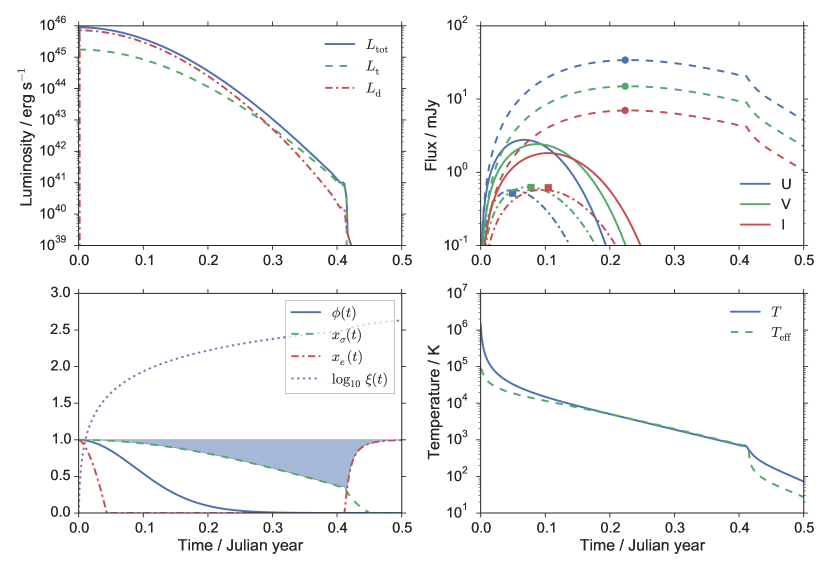
Figure 3: Simulated quantities for an outburst with nominal parameters (see Section 2) and $\beta=0.2$. Upper left panel displays total, diffusive and optically thin luminosities ($L_{\text{tot}}$, $L_{\text{d}}$ and $L_{\text{t}}$, respectively). Upper right panel shows optical fluxes in $U$, $V$ and $I$-bands (assuming the nominal luminosity distance of $D_{L}=1500\,$\mathrm{M}\mathrm{p}\mathrm{c}$$). Model output is indicated with solid lines, the estimates from equations (63), (66) and (67) with dashed lines and filled circles, and estimates from equations (70) and (71) with dash-dotted lines and filled squares. Bottom left panel shows the time evolution of $\xi$, $\phi$ and the relative photospheric radii $x_{\sigma}$ and $x_{e}$ corresponding to the electron scattering and effective optical thicknesses respectively. The shaded blue region indicates the optically thin extent at each time. Bottom right panel depicts time evolution of the model temperature $T$ as defined by equation (35) and the effective temperature $T_{\text{eff}}$ defined by (53).

Using the same assumptions, we can also make estimates for the spectral peak and the flux at the peak for a black body. The position of the spectral peak is proportional to the effective temperature, so

$$\begin{split}\nu^{\prime}_{\text{peak,BB}}&\sim 5.879\times 10^{10}\,\frac{1+\beta}{1+z}T_{\text{eff}}(0)\,\xi(t_{e})^{-1/2}\phi(t_{e})^{1/4}\,$\mathrm{H}\mathrm{z}$\\ &=7.2\times 10^{15}\,\frac{1+\beta}{1+z}\,$\mathrm{H}\mathrm{z}$\\ &\quad\times h_{15}^{-1/12}M_{8}^{-1/6}r_{10}^{-5/12}\delta^{5/6}\xi(t_{e})^{-1/2}\phi(t_{e})^{1/4}.\end{split}$$ (68)

Based on this we can say that (66) and (67) are usable only in the limit $\nu^{\prime}\ll\nu^{\prime}_{\text{peak,BB}}$. The flux at peak is

$$\begin{split}\frac{F^{\prime}_{\nu^{\prime}_{\text{peak}},BB}}{1+z}&\sim\frac{\pi}{D_{L}^{2}}\,1.896\times 10^{10}\,$\mathrm{m}\mathrm{J}\mathrm{y}\,\mathrm{K}^{-3}$\,T_{\text{eff}}(0)^{3}R_{0}^{2}\\ &\quad\times\xi(t_{e})^{1/2}\phi(t_{e})^{3/4}\int_{0}^{\theta^{\prime}_{\text{max}}}D(\theta)^{3}\sin(2\theta)\mathrm{d}\theta\\ &\sim 0.23\,(1+2\beta)\,$\mathrm{m}\mathrm{J}\mathrm{y}$\\ &\quad\times h_{15}^{5/12}M_{8}^{5/6}r_{10}^{1/12}\delta^{-1/6}D_{L,1500}^{-2}\\ &\quad\times\xi(t_{e})^{1/2}\phi(t_{e})^{3/4}.\end{split}$$ (69)

In principle, we can also estimate the maximum flux using the black body assumption, if we additionally assume $t_{\text{h}}\ll t_{\text{d}}$ and $\beta\sim 0$. In this case, the flux is given by

$$F^{\prime}_{\nu^{\prime}}(t^{\prime})=\frac{(1+z)\pi}{D_{L}^{2}}R(t_{e})^{2}B_{(1+z)\nu^{\prime}}(T_{\text{eff}}(t_{e})).$$ (70)

The maximum flux is

$$\begin{split}\frac{F^{\prime}_{\nu^{\prime},\text{max,BB}}}{(1+z)^{4}}&=\frac{\pi}{D_{L}^{2}}\frac{R(t_{e})^{2}2h\nu^{\prime 3}/c^{2}}{\exp\left[\frac{(1+z)h\nu^{\prime}}{kT_{\text{eff}}(0)}\xi(t_{e})^{1/2}\phi(t_{e})^{-1/4}\right]-1}\\ &\sim 1.6\times 10^{-3}\,$\mathrm{m}\mathrm{J}\mathrm{y}$\,f(\xi)\\ &\quad\times M_{8}^{4/3}h_{15}^{2/3}n_{14}^{1/2}r_{10}^{4/3}\delta^{-8/3}D_{L,1500}^{-2}\nu_{550}^{3},\end{split}$$ (71)

where

$$f(\xi) =\xi^{2}\left\{\exp\left[C_{1}\xi^{1/2}\exp(-C_{2}(\xi^{2}-1))^{-1/4}\right]-1\right\}^{-1}$$ (72)

$$C_{1} =0.21(1+z)M_{8}^{1/6}h_{15}^{1/12}r_{10}^{5/12}\delta^{-5/6}\nu_{550}$$ (73)

$$C_{2} =1.7\times 10^{-5}\beta^{-1}M_{8}^{-2/3}h_{15}^{-1/3}n_{14}^{-1}r_{10}^{-2/3}\delta^{4/3}.$$ (74)

This flux maximum is determined by maximum of $f$, for which no convenient analytic result exists. For nominal parameter values and $\beta=0.2$ we can numerically find $\xi_{\text{max}}\sim 72$, which gives $t_{\text{max}}\sim 72t_{\text{h}}$ and $f(\xi_{\text{max}})\sim 430$. Thus, the estimate for nominal $V$-band maximum brightness is $\sim 1.8\,$\mathrm{m}\mathrm{J}\mathrm{y}$$.

We can compare these estimates to Figures 3 and 4, which depict the model results for an example outburst with nominal parameter values and a moderate value of $\beta=0.2$. The effect of Doppler boosting through $\beta$ can be clearly seen in the flux light curves when compared to the blackbody estimate of equation (70). Otherwise, using the naive blackbody value for flux is a good approximation. On the contrary, the Rayleigh–Jeans estimates from (66) and (67) are inaccurate at optical wavelenghts. The estimate for maximum flux is too high by a factor of few. Likewise, the estimated time-scale of the outburst is too long. This is not surprising, since during the brightest part of the outburst, the spectral peak is at optical frequencies as well, and the Rayleigh–Jeans assumption does not hold.

The Figure 4 clearly visualizes how the initial spectral evolution is dominated by the hydrodynamical time-scale through expansion and adiabatic cooling, resulting in an increasing peak flux at smaller peak frequencies. After $t\sim\sqrt{t_{\text{d}}t_{\text{h}}}$, photon diffusion cools the gas and the maximum flux and the peak frequency diminish quickly. The estimates given by equations (68) and (69) are reasonably good.

During most of the outburst, the diffusive luminosity dominates the optically thin luminosity by approximately an order of magnitude. At later times, when the bubble has rarefied enough, the optically thin luminosity exceeds the diffusive contribution. However, soon after this, the low temperature induces a quick rise in the effective optical depth, quenching the optically thin contribution to luminosity. It is clear that for nominal parameter values, the optically thin luminosity is only a minor component of the total luminosity. However, as noted in Section 3.1, a pre-existing or expansion induced density gradient could enhance the optically thin contribution.

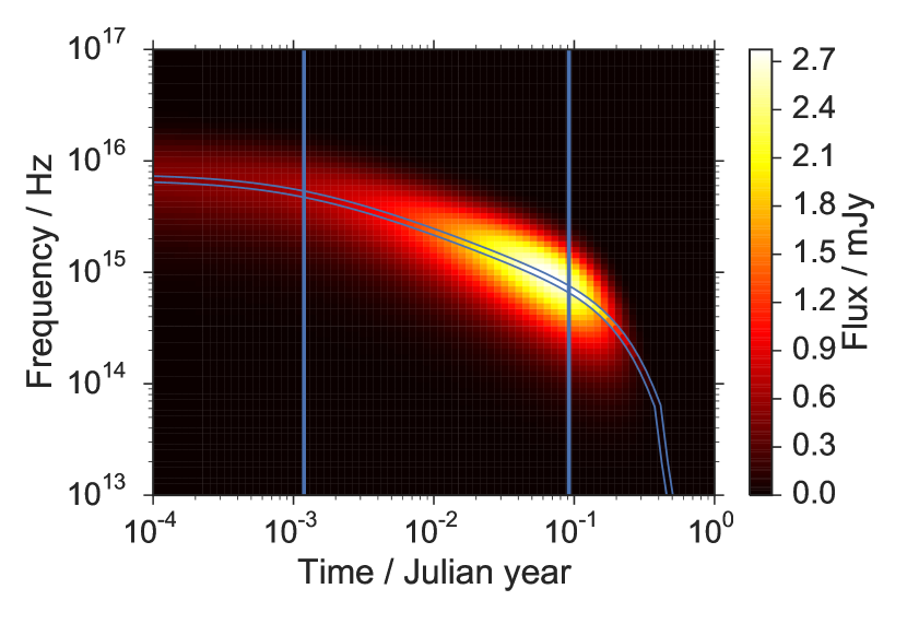
Figure 4: Time evolution of the observed spectrum for an outburst with nominal parameters and $\beta=0.2$. Note the logarithmic scale on the $x$-axis. The curved blue lines bracket the estimate of the spectral peak position, given by equation (68), and the flux at spectral peak, given by equation (69). The two vertical lines indicate the time-scales $t_{\text{h}}$ and $\sqrt{t_{\text{h}}t_{\text{d}}}$ from left to right, respectively.

4 Accretion disc impacts as an observational tool

When the outburst model is tied to physical parameters at the impact site through estimates in Section 2, we can use the model to probe the physical parameters of the accretion disc through $h_{15}$ and $n_{14}$, and the orbital parameters and mass of the impactor through $r_{10}$, $M_{8}$ and the outburst timings. In constructing the model, the nominal values of these parameters were chosen to represent the scenario originally presented in LV96. Since the mass of the primary in LV96 model and its later developments is high, $\sim 10^{10}\,M_{\odot}$, nominal parameter values are not representative of the general SMBH population.

To properly estimate the possibility of observing accretion disc impact outbursts, we construct a large number of impact scenarios based on observational data of quasars. Quasars form a convenient benchmark, since it is well established that they represent a population of SMBHs, and that their luminosity is powered by matter accretion through a disc (e.g. Malkan, 1983). Furthermore, quasar activity is commonly linked to galaxy merger events – e.g. Johansson et al. (2009); Treister et al. (2012), but see also Cisternas et al. (2011) – which makes the existence of a close binary of SMBHs within a quasar a plausible scenario. Indeed, there are now several promising candidates detected with a variety of methods (Sillanpää et al., 1988; Graham et al., 2015a; Liu et al., 2015; Graham et al., 2015b). We compare the maximum outburst luminosity and flux calculated using our accretion disc impact model with the quiescent (baseline) luminosity and flux of the quasar to assess how likely it is that the outburst could be observed.

For our data, we use the observations of 62185 SDSS quasars in Steinhardt & Elvis (2010). This data yields the mean masses and luminosities in 9 evenly spaced redshift bins from $z=0.2$ to $z=2.0$. The paper also presents evidence for a redshift-dependent luminosity limit for quasars of the form

$$\log L_{\text{max}}=\alpha(z)\log M+\log L_{0}(z),$$ (75)

which the authors dub the sub-Eddington limit, due to the result that $\alpha<1$ in all the observed redshift bins. For each redshift bin, we construct a sample of quasars by sampling the black hole masses from a normal distribution assuming the given mean and standard deviation for each bin. The quasar luminosities are then set to the maximum expected luminosity given by the equation (75) to yield conservative estimates when compared to the accretion disc impact luminosities. The quasar redshift is generated from a uniform distribution over the redshift bin size. We have reproduced the required values in Table 1, where it should be noted that for the redshift bin $z=0.6$–$0.8$, where two sets of values are available, we have used the values derived using the H$\beta$ line.

Table 1: Mean quasar mass $\langle M\rangle$, mass standard deviation $\sigma_{M}$ and the sub-Eddington limit coefficients $\alpha$ and $L_{0}$ for each redshift bin, from Steinhardt & Elvis (2010).

Redshift	$\langle\log(M/M_{\odot})\rangle$	$\sigma_{M}$	$\alpha$	$L_{0}$
0.2-–0.4	8.27	0.44	0.37	42.63
0.4-–0.6	8.44	0.42	0.45	42.13
0.6-–0.8	8.69	0.39	0.60	41.07
0.8-–1.0	8.76	0.31	0.67	40.60
1.0-–1.2	8.89	0.29	0.67	40.71
1.2-–1.4	8.96	0.29	0.73	40.24
1.4–1.6	9.07	0.28	0.68	40.66
1.6–1.8	9.18	0.29	0.50	42.35
1.8-–2.0	9.29	0.30	0.42	43.20

For each constructed quasar, we assume a standard Shakura–Sunyaev accretion disc (Shakura & Sunyaev, 1973) with $\alpha=0.1$, which is consistent with observations (King et al., 2007). The disc mass accretion rate is set to $\dot{M}=(L/L_{\text{Edd}})\dot{M}_{\text{Edd}}$. We then compute the model outputs using impact distances $r_{10}=1$ and $r_{10}=10$, while setting $\delta=1$. The outflow velocity $\beta$ is set equal to the impact velocity, $\beta=v_{\text{r}}/c=(10r_{10})^{-1/2}$. The mass ratio $q$ of the impacting black hole to the quasar black hole is set in turn to $0.1$, $0.3$ and $1.0$. The resulting maximum outburst luminosity is found at $t=0$, as outlined in Section 3. The maximum flux at $510\,$\mathrm{n}\mathrm{m}$$ (in observer frame) is found by numerical maximisation procedure. This is compared against the quasar flux at the same observed wavelength. This is derived by using observed bolometric corrections in reverse. We compute the observed flux from

$$F_{\nu}=\frac{1+z}{4\pi D_{L}^{2}}\frac{1}{\nu}\left(\lambda L_{\lambda}\right),$$ (76)

where $\lambda=510\,$\mathrm{n}\mathrm{m}$$ and $\nu=c/\lambda$. The value of $\lambda L_{\lambda}$ is obtained using the bolometric correction relations in Runnoe et al. (2012), which give

$$\log(L_{\text{iso}})=4.89+0.91\log(\lambda L_{\lambda}),$$ (77)

where $\lambda=510\,$\mathrm{n}\mathrm{m}$$ is the observed wavelength and $L_{\text{iso}}$ is the isotropic luminosity of the quasar, which is taken to be equal to the bolometric luminosity determined above. For each redshift bin we generate a sample of $N=1000$ quasars, compute the impact model for each combination of $r_{10}$ and $q$, and finally derive the resulting ratios of maximum luminosity and maximum flux ratios for observed wavelength $\lambda=510\,$\mathrm{n}\mathrm{m}$$.

Table 2: Fraction of impacts exceeding the simulated quasar bolometric luminosity in each redshift bin, for each mass ratio and impact distance $r_{10}$.

Mass ratio	$0.1$		$0.3$		$1.0$
$r_{10}$	1	10	1	10	1	10
Redshift
0.2–0.4	0.1%	0.0%	6.4%	0.1%	63.1%	7.5%
0.4–0.6	0.0%	0.0%	1.4%	0.0%	56.8%	1.7%
0.6–0.8	0.0%	0.0%	0.0%	0.0%	33.7%	0.0%
0.8–1.0	0.0%	0.0%	0.0%	0.0%	2.8%	0.0%
1.0–1.2	0.0%	0.0%	0.0%	0.0%	0.3%	0.0%
1.2–1.4	0.0%	0.0%	0.0%	0.0%	0.0%	0.0%
1.4–1.6	0.0%	0.0%	0.0%	0.0%	0.4%	0.0%
1.6–1.8	0.0%	0.0%	0.0%	0.0%	3.8%	0.0%
1.8–2.0	0.0%	0.0%	0.0%	0.0%	3.4%	0.0%

Table 3: Fraction of impacts exceeding the simulated quasar flux at $\lambda=510\,$\mathrm{n}\mathrm{m}$$ in each redshift bin, for each mass ratio and impact distance $r_{10}$.

Mass ratio	$0.1$		$0.3$		$1.0$
$r_{10}$	1	10	1	10	1	10
Redshift
0.2–0.4	1.7%	15.2%	13.8%	65.8 %	53.2%	97.1%
0.4–0.6	0.5%	2.5%	13.6%	56.1 %	59.9%	98.0%
0.6–0.8	0.1%	0.0%	5.7%	12.8 %	64.5%	98.7%
0.8–1.0	0.0%	0.0%	0.2%	0.0 %	53.3%	97.4%
1.0–1.2	0.0%	0.0%	0.1%	0.0 %	53.9%	55.5%
1.2–1.4	0.0%	0.0%	0.0%	0.0 %	48.5%	1.5%
1.4–1.6	0.0%	0.0%	0.4%	0.0 %	73.7%	2.9%
1.6–1.8	0.0%	0.0%	2.7%	0.0 %	71.4%	6.9%
1.8–2.0	0.0%	0.0%	3.1%	0.0 %	65.5%	2.1%

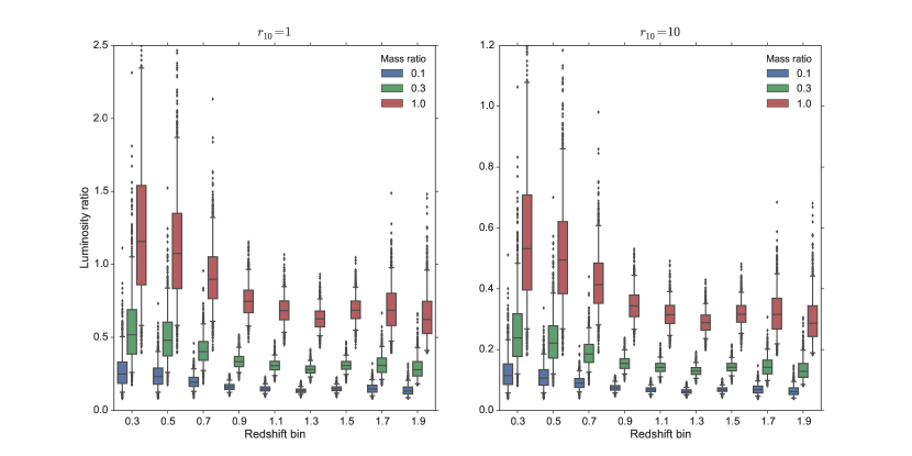
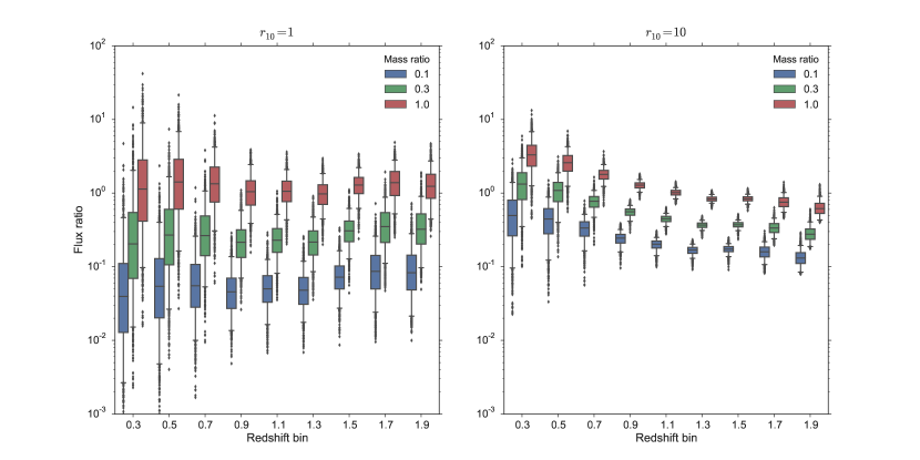
Figure 5: Top figure shows the ratio of the maximum impact outburst bolometric luminosity to the quasar bolometric luminosity as a function of redshift bin center Bottom figure shows the ratio of the maximum outburst flux at $\lambda=510\,$\mathrm{n}\mathrm{m}$$ to the quasar flux at the same observed wavelength. The impacts are calculated for $r_{10}=1$ (left column) and $r_{10}=10$ (right column) and mass ratios $q\in[0.1,0.3,1.0]$, indicated by blue, green and red colours respectively. The boxes extend from first to third quartile, with a line indicating the median value. The whiskers extend from 5th to 95th percentile, with outlier values indicated by isolated points. Note the logarithmic $y$-axis scaling in the lower plot.

The results are depicted graphically in Figure 5. In addition, the fraction of impact outbursts that equal or exceed the quasar bolometric luminosity or flux at $\lambda=510\,$\mathrm{n}\mathrm{m}$$ are listed in Tables 2 and 3. While the impact outburst luminosity can exceed the quasar luminosity, this is only likely for high mass ratios, small impact distances and lower redshifts. The luminosity ratio distribution does have a long tail with outliers with up to a ratio of 5 for $r_{10}=1$ and $q=1.0$. However, the observed flux at $\lambda=510\,$\mathrm{n}\mathrm{m}$$ from the impact outburst can exceed the quasar flux by more than an order of magnitude. For $q=1$, the median outburst flux is equal to the quasar flux up to $z=1.8\text{--}2.0$, and up to $z=0.4\text{--}0.6$ for $q=0.3$. From the above, we conclude that combined with the expected spectral evolution discussed in Section 3.4, it should be possible to discern impact outbursts from the normal quasar stochastic variability using observations in the optical frequencies.

4.1 Observational complications and secondary effects

The physics of the interaction between a black hole and the accretion disc present some complications to the idealized observational picture presented above. Furthermore, the sequence of impacts can have observable effects on a larger (galactic) scale as well. We will briefly consider these in the following.

A central question is the effect of the secondary companion on the of the accretion disc of the primary. If disc and binary co-align, or the disc is disrupted, the sequence of observable discrete impacts will cease. In general, it is known that a circumbinary disc and the binary orbital plane will eventually align (Ivanov et al., 1999; Lodato & Pringle, 2006; Nixon, 2012), possibly through violent tearing of the disc (Nixon et al., 2012, 2013). However, we are specifically interested in the case where a circumbinary cavity has not yet formed. Precisely this situation was investigated in Ivanov et al. (1999). They found that the accretion disc impacts would continue until the disc interior to the binary aligns with the binary orbital plane. They estimate the alignment to happen on a time-scale

$$\frac{t_{a}}{P_{\text{orb}}}\sim\frac{M_{2}}{2\pi\Sigma R_{\text{BH}}^{2}A}\sim 5.2\times 10^{10}\,A^{-1}\alpha\dot{m}M_{8}^{-1}r_{10}^{-7/2}\delta^{4},$$ (78)

where $t_{a}$ is the alignment time-scale, $P_{\text{orb}}$ is the binary orbital period, $\Sigma$ is the accretion disc surface density, $\dot{m}=\dot{M}/\dot{M}_{\text{Edd}}$, the constant $A>1$ depends on the disc response on scales larger than $R_{\text{BH}}$, and we have used the inner, radiation pressure dominated solution for $\Sigma$. This is valid for impacts up to $r_{10}\sim 400\dot{m}^{16/21}(\alpha M_{10})^{2/21}$ (Shakura & Sunyaev, 1973). We find that the alignment time is sufficiently long for extended series of impact outbursts to occur.

However, the impacts also deplete the accretion disc of gas. This may lead to a lower steady state surface density of the disc. This would impact the time-scale of the outbursts, but the maximum luminosity (see equation (62)) would not be much affected. This is because the lower energy density is compensated by the shortened diffusion time-scale. The peak flux densities at a given wavelength would be expected to decrease, however. Nevertheless, if the depletion is fast enough, a cavity will be excavated and the outbursts will cease. Ivanov et al. (1999) give an approximate condition for negligible depletion in terms of the mass ratio $q$,

$$q<\sqrt{\frac{3\pi}{4}}\alpha^{1/2}\frac{h}{r}\sim 1.7\,\alpha^{1/2}\dot{m}r_{10}^{-1}(1-0.55r_{10}^{-1/2}),$$ (79)

where $h/r$ is the disc opening angle. We see that e.g. for the high luminosity quasars ($\dot{m}\sim 1$) considered above, the disc accretion rate is sufficient to maintain the theoretical $\alpha$-disc surface density at $r_{10}=10$ for up to $q\sim 0.04$. For higher mass ratios, when the condition is violated, the steady state surface density can be expected to decrease to a value (Ivanov et al., 1999)

$$\Sigma=\alpha q^{-2}\left(\frac{h}{r}\right)^{2}\Sigma_{0}\sim 1.2\,\alpha q^{-2}\dot{m}^{2}r_{10}^{-2}(1-1.1r_{10}^{-1/2}),$$ (80)

where $\Sigma_{0}$ is the unperturbed steady state surface density. For $\alpha=0.1$, $r_{10}=10$ and $\dot{m}\sim 1$ we find $\Sigma\sim 8\times 10^{-4}\,q^{-2}\Sigma_{0}$. This is reasonably small, even for mass ratios up to $q=0.1$. We may conclude that a train of accretion disc impact outbursts can continue for a significant amount of time, if the binary mass ratio is modest ($q\lesssim 0.1$) and the impacts happen near the inner regions of the accretion disc of the primary. For larger mass ratios, we expect the impact sequence to diminish in brightness with a characteristic minimum time-scale of approximately

$$t_{\text{dim}}\sim 5.3\times 10^{11}\,\dot{m}^{-2/3}M_{10}^{7/3}M_{8}^{-4/3}r_{10}^{11/3}\delta^{8/3}\,$\mathrm{s}$,$$ (81)

derived by dividing the accretion disc mass inside the binary orbit by the approximate rate of matter expulsion by the binary, $\sim 2\pi(R_{0}^{\text{LV}})^{2}\Sigma_{0}/P_{\text{orb}}$. From this, we can estimate the number of observable outbursts before significant reduction in the disc surface density. We find

$$\frac{2t_{\text{dim}}}{P}\sim 5.4\times 10^{4}\,\dot{m}^{-2/3}M_{10}^{4/3}M_{8}^{-4/3}r_{10}^{13/6}\delta^{8/3},$$ (82)

and conclude that even for $q=1$ the estimate yields around $10^{2}$ outbursts before the inner disc is depleted. However, as a final remark, we caution that for $q\sim 1$, the secondary may violently disrupt the inner disc on time-scales that are faster than the estimates above.

A related complication is that as the impacts modulate the structure of the accretion disc, they can affect the accretion rate and thus the luminosity of the primary SMBH. This luminosity change would be apparent approximately after one sound-crossing time of disc,

$$t_{\text{sc}}=\frac{r}{c_{s}}\sim\frac{r^{2}}{hv_{\text{K}}}\sim 2.9\times 10^{6}\dot{m}^{-1}M_{10}r_{10}^{5/2}\,$\mathrm{s}$.$$ (83)

Typically $t_{\text{sc}}\lesssim P_{\text{orb}}$, and observations of the impact sequence will be complicated by the changing accretion rate of the primary. An estimate for the change in the primary accretion rate can be obtained from the results of Kumar & Johnson (2010), who considered the effect of supernova explosions in an accretion disc. Using their results yields a mean increase in the primary accretion rate of

$$\Delta\dot{M}\sim 4\times 10^{-3}\,q^{2.2}M_{10}^{-0.25}h_{15}^{1.1}n_{14}^{0.85}r_{10}^{-0.075}\delta^{-2.2}\,\dot{M}_{\text{Edd}}.$$ (84)

The corresponding change in luminosity is small compared to the impact luminosity, which can be $\sim qL_{\text{Edd}}$. The change in primary black hole luminosity also decreases faster with diminishing mass ratio. We thus expect that the impact outbursts would not be completely overshadowed by the changes in the primary black hole luminosity.

Finally, there is the possibility that the impact may eventually cause a wind-like outflow to form. This is dependent on the velocity to which the outflow is accelerated. The impact velocity is $v_{\text{r}}=\sqrt{2}\delta v_{\text{K}}$, and by the discussion in Section 2 we expect the outflow to reach velocities higher than this. For high-inclination impacts, this is then above the escape velocity. In this case, the outflow will eventually turn over into a Sedov-Taylor blastwave. At the time when the radiative losses become important, the outflow has reached a distance of

$$R_{\text{rad}}\sim 210\,M_{8}^{10/17}n_{14}^{5/17}r_{10}^{5/17}\delta^{-10/17}n_{0}^{-1/5}\,$\mathrm{p}\mathrm{c}$$$ (85)

at a velocity of

$$v_{\text{rad}}\sim 290\,M_{8}^{2/17}n_{14}^{1/17}r_{10}^{1/17}\delta^{-2/17}n_{0}^{-1/5}\,$\mathrm{k}\mathrm{m}\,\mathrm{s}^{-1}$,$$ (86)

where $n_{0}=n/(1\,$\mathrm{c}\mathrm{m}^{-3}$)$ is the gas density in the galaxy nucleus. Since the estimates above are lower limits, and likely $n_{0}\lesssim 0.1$ (Mathews & Brighenti, 2003), we see that the impact sequence can create a wind at $\sim$\mathrm{k}\mathrm{p}\mathrm{c}$$ scales, moving at velocities of $\sim 500\,$\mathrm{k}\mathrm{m}\,\mathrm{s}^{-1}$$.

We can conclude that particularly binaries with mass ratios $\lesssim 0.05$ can yield impact flare sequences that last for very long times, and thus should in principle be observable. Furthermore, evidence for a history of accretion disc impacts in galactic nucleus can possibly be imprinted in winds originating from the nucleus. To complete the discussion, we examine the assumptions made in building the analytic model of the disc impact scenario itself in the next section.

5 Discussion

The physical situation during an accretion disc impact in a supermassive binary black hole system, such as OJ287, is obviously more complex than what is assumed in LV96, I98 or this work. However, little analytic progress can be made unless several simplifying assumptions are made. Explicitly listed, the significant assumptions shared by all these models are:

1. spherical symmetry

2. adiabatic expansion into empty space

3. constant temperature profile

4. constant density profile

5. gravitational effects are negligible

6. negligible magnetic fields

7. negligible radiation from the accretion disc.

We will discuss the possible effects these assumptions may have on the validity of the model results.

The hydrodynamical simulations in I98 show that spherical symmetry is actually a rather good approximation for the problem. A steep density gradient in the disc can be expected to produce a more conical outflow, but this conicality will be partly masked by the relativistic restrictions on the visible angular extent of the photosphere. However, I98 also find that the density profile of the outflow sphere is given by a steep power law, $\rho\propto R^{-5}$. If this is true, the outer layers would be less dense than in the homogeneous case, decreasing their optical thickness. This decrease is partly balanced by the fact the outer layers should also be somewhat cooler, both initially and during the evolution. This will tend to increase the opacity when temperatures are in the region dominated by Kramers’ law. In this sense, the compromise of homogeneous density and temperature profiles is acceptable.

The gravitational effects of the accretion disc and the primary on the evolution of the outflow gas are difficult to quantify. However, at least for impacts happening close to the primary, neglecting gravitational effects is likely not a good approximation, whereas the gravitational perturbation caused by the accretion disc is negligible compared to the black holes. Strong gravity near the primary would certainly distort the outflow into an asymmetric shape. This geometric distortion might affect both peak luminosity and outburst time-scale due to decreased diffusion time and earlier onset of optical thinness. More importantly, as investigated in e.g. Karas & Vokrouhlicky (1994) and Dai et al. (2010), the gravitational lensing effect might increase the observed flux by a large factor. The observed spectrum would also be affected by the differences in light travel times from different parts of the outflow, as well as gravitational redshift.

Observations and models suggest that non-negligible magnetic fields exist near the inner parts of the accretion disc and threading the central black hole in luminous AGN (Eatough et al., 2013; Sikora & Begelman, 2013; Silant’ev et al., 2013; Zamaninasab et al., 2014; Martí-Vidal et al., 2015). Unfortunately, the expected magnetic field strengths are not well constrained, and the degree of ordering is likewise uncertain (King et al., 2007; McKinney & Narayan, 2007; Tchekhovskoy et al., 2011). Nevertheless, even a disordered magnetic field would still produce a synchrotron component in the observed radiation. The synchrotron emission would serve to convert some of the plasma kinetic energy to radiation, likely increasing the outburst duration. However, in the case of OJ287, there is evidence that outbursts associated with accretion disc impacts are associated with lower degree of polarization (Valtonen et al., 2008). This indicates that synchrotron emission is not a major component during these outbursts.

The accretion disc serves not only as the source of the outflow material, but it also illuminates it and reflects the outflow radiation back. These effects are difficult to estimate analytically, though we may assume that they are significant especially near the hot inner regions of the accretion disc.

Lastly, the assumption of expansion into free space is not unproblematic either, since it is commonly assumed that accretion discs are embedded in hot coronae. This corona of hot rarified gas might comptonize the radiation from the outflow. Furthermore, while an accretion disc corona is usually expected to be rarified, this might not be the case if recurrent impacts have separated a significant amount of matter from the accretion disc to the corona. This matter might then serve to both cloud the outflow from view, and decelerate the outflow, turning a linear expansion into a Sedov–Taylor power law.

The discussion above may cast doubt on whether any analytic model can be expected to describe the accretion disc impact outflows to any degree of accuracy. To make a case that this is possible, we should first note that if the impact site is distant from the primary black hole, all of the assumptions with the exception of (iii) and (iv) are valid. And, as already noted, even if assumptions (iii) and (iv) are violated, this should not greatly affect the luminosity or the spectral evolution, at least initially. When the impact site is taken to be progressively closer to the primary, the assumptions will break down, but only gradually, to some order of $r_{10}$. Even near the primary Schwarzschild radius at $r_{10}=0.1$ we may expect the estimated luminosity to be of the correct order, even though the evolution of observed flux may have diverged completely from the model estimates. In conclusion, despite the caveats mentioned above, we expect the model to have good predictive power in much of the SMBH binary orbital parameter space.

6 Conclusions

We have estimated the physical characteristics of an impact by a supermassive black hole on the accretion disc of another supermassive black hole. We have compared our results to earlier studies, with a focus on the LV96 paper, and we find that an impact would cause an expanding outflow to form. This outflow expands at a mildly relativistic velocity, and is observable very soon after the initial impact, with most of the radiation escaping through diffusion.

Building on these estimates, we have developed a model for the spectral evolution of such an impact outflow. The model is based on time-dependent photon diffusion and takes into account the emission from optically thin regions. The observed flux is then corrected for relativistic effects. In addition to the model, we present approximate analytic formulae for estimating maximum luminosity, maximum flux and the relevant time-scales, correct to first order in outflow expansion velocity $\beta$.

The model was applied to simulated populations of quasars in a redshift range $z=0.2\text{--}2.0$, constructed by using observed quasar statistics. The quasars were assumed to host SMBH binaries with a selection of mass ratios and orbital radii, and the accretion disc parameters of the primary black hole were estimated with thin $\alpha$-disc theory. The maximum luminosity and the flux at the observed wavelength $\lambda=510\,$\mathrm{n}\mathrm{m}$$ resulting from the accretion disc impact model for each configuration were computed. The model results were compared to the quasar bolometric luminosity and flux at the same observed wavelength. The quasar luminosities were set to the sub-Eddington limit (see Steinhardt & Elvis (2010) and Section 4), and the quasar fluxes were derived using the bolometric corrections in Runnoe et al. (2012). The results indicate that detecting impact flares should be possible, as the impact flares can peak at flux densities that are several times the value of the quasar flux, and can be comparable up to high redshifts with moderate binary mass ratios. As such, searching for impact outbursts might serve as an independent method for locating SMBH binaries in active galactic nuclei.

Finally, we have extensively discussed the simplifying assumptions that have been made in producing the model and the analytic results for the impact outflows. While most of the assumptions are violated for impacts happening near the primary black hole, we expect that in most cases our model should give a good description of the outburst. However, it should be emphasized that the problem would greatly benefit from a comprehensive assessment with state of the art numerical simulations.

Appendix A Symbol list

Table 4 lists most of the mathematical symbols used in the paper with explanations. The table is divided into sections that roughly correspond to the sections of the paper. Within the sections, the symbols are listed in the order of appearance, where feasible.

Table 4: A summary of the symbols used in the paper.

Symbol	Description	Symbol	Description
Black hole binary & accretion disc
$M_{10}$	Primary black hole mass / $10^{10}M_{\odot}$	$h_{15}$	Accretion disc semiheight / $10^{15}$\mathrm{c}\mathrm{m}$$
$M_{8}$	Secondary black hole mass / $10^{8}M_{\odot}$	$n_{14}$	Accretion disc number density / $10^{14}\,$\mathrm{c}\mathrm{m}^{-3}$$
$r_{S,1}$	Primary black hole Schwarzschild radius	$D_{L,1500}$	Luminosity distance / $1500\,$\mathrm{M}\mathrm{p}\mathrm{c}$$
$r_{10}$	Distance from the primary black hole / $10r_{S,1}$	$z$	Redshift
Impact shock
$k$	Boltzmann constant	$n_{2}$	Post-shock number density
$\sigma_{T}$	Thomson electron scattering cross section	$x$	Gas compression factor
$\kappa_{T}$	Thomson electron scattering opacity	$\gamma_{a}$	Adiabatic constant
$\sigma_{B}$	Stefan-Boltzmann constant	$\gamma$	Electron Lorentz gamma factor
$a$	Radiation constant, $4\sigma_{B}/c$	$\beta$	Lorentz beta
$m_{p}$	Proton mass	$t_{\text{ff}}$	Bremsstrahlung cooling time-scale
$m_{e}$	Electron mass	$t_{\text{IC}}$	Inverse Compton cooling time-scale
$v_{\text{K}}$	Keplerian orbital velocity of the impactor	$\epsilon^{\text{ff}}_{\nu}$	Bremsstrahlung volume emissivity
$v_{\text{r}}$	Relative velocity of impactor and accretion disc gas	$\epsilon^{\text{ff}}$	Integrated bremsstrahlung volume emissivity
$\theta_{\text{i}}$	Inclination angle between the binary orbital plane and the accretion disc	$\epsilon_{\text{IC}}$	Inverse Compton volume emissivity
$\delta$	Inclination parameter, $\sqrt{1-\sin\theta_{\text{i}}}$	$T_{\text{eq}}$	Shock equilibrium temperature
$c_{s}$	Speed of sound in the accretion disc	$\mathcal{M}_{1}$	Shock mach number
$t_{\text{dyn}}$	Dynamical time-scale of the impact event	$\mathcal{M}_{e,1}$	Shock effective mach number
$T_{\text{disc}}$	Accretion disc temperature	$P_{\text{g}}$	Gas pressure
$T_{\text{vir}}$	Accretion disc temperature	$P_{\text{r}}$	Radiation pressure
$n$	Pre-shock number density	$R_{P}$	Ratio of radiation to gas pressure
Outflow
$R_{0}^{\text{I98}}$	Initial outflow radius according to I98	$V_{0}$	Initial outflow volume
$R_{0}^{\text{LV96}}$	Initial outflow radius according to LV96	$\lambda$	Ratio of secondary Bondi–Hoyle radius to accretion disc semiheight
$R_{0}^{\text{sim}}$	Initial outflow radius estimated from I98 simulations	$L_{\text{Edd}}$	Eddington luminosity
$R_{\text{BH}}$	Bondi–Hoyle radius of the secondary black hole	$t_{\text{d}}$	Photon diffusion time-scale
LV96 model
$P$	Total pressure	$\xi_{\text{ff}}$	Expansion factor when $\tau_{\text{a}}=1$
$\rho$	Gas density	$\xi_{\text{T}}$	Expansion factor when $\tau_{\sigma}=1$
$R$	Radial size of the outflow bubble	$t_{0}$	Time delay between the impact and the outflow turning optically thin
$T$	Temperature of the outflow bubble	$S_{V}$	Flux density in the optical $V$-band
$u_{1}$, $u_{2}$	Pre- and post-shock velocities of the gas in shock frame	$t_{\text{outb}}$	Length of the outburst
$v_{2}$	Post-shock gas velocity in observer frame	$\psi_{\text{ff}}$	Bremstrahlung volume emissivity exponential cutoff parameter
$\xi(t)$	Relative expansion factor $R(t)/R_{0}$	$W_{-1}$	The $-1$ branch of the Lambert W function
$\mu$	Mean molecular weight	$T_{e}$	Electron temperature
$t_{\text{h}}$	Hydrodynamical, or expansion time-scale	$y$	The comptonization parameter
$\tau_{\text{e}}$	Effective optical depth	$T_{\text{eff}}$	Effective black body temperature
$\tau_{\text{a}}$	Optical depth of absorption processes	$\epsilon$	Dilution factor of the diluted black body spectrum
$\tau_{\sigma}$	Electron scattering optical depth	$E_{r}$	Radiative energy
$\kappa_{a}$	Kramers’ law of opacity	$\eta$	Ratio of radiative energy to matter rest energy
$K_{a}$	The constant factor of Kramers’ law	$L_{\text{t}}$	Optically thin luminosity
$\xi_{\text{LV}}$	Expansion factor when $\sqrt{\tau_{\text{a}}\tau_{\sigma}}=1$	$L_{\text{d}}$	Optically thick, diffusive luminosity
New model
$\kappa$	Opacity	$L_{\text{tot}}$	Total luminosity
$x$	Relative radial distance, $x=r/R(t)$	$l$	Photon mean free path
$\psi(x)$	Dimensionless temperature profile	$\tau_{p}$	Optical depth of the photosphere
$\phi(t)$	Thermal energy time dependency	$x_{\sigma}$	Relative radial distance at which $\tau_{\sigma}=\tau_{p}$
$\alpha$	Diffusion equation eigenvalue	$x_{e}$	Relative radial distance at which $\tau_{\text{e}}=\tau_{p}$
$\eta(x)$	Dimensionless density profile	$x_{p}$	Relative radial distance of the photosphere
$M(x)$	Total mass within $x$	$t_{c}$	Generic cooling time-scale
$I_{M}(x)$	Density distribution form factor	$\beta$	Expansion velocity / $c$
$E_{T}(x,t)$	Thermal energy within $x$ at time $t$	$\Gamma$	Expansion Lorentz gamma factor
$I_{T}(x)$	Thermal energy distribution form factor	$t_{e}$	Emission time

Appendix B Code

A Python/Cython computer code was constructed to perform the model computations used in the paper. This code is freely available at https://bitbucket.org/popiha/impact_model. The code can be used to compute the accretion disc impact spectrum at given frequencies, as well as other model quantities as a function of time. Detailed information and instructions for use are provided with the code.

References

- Alig et al. (2011) Alig C., Burkert A., Johansson P. H., Schartmann M., 2011, MNRAS, 412, 469
- Aly et al. (2015) Aly H., Dehnen W., Nixon C., King A., 2015, MNRAS, 449, 65
- Armitage et al. (1996) Armitage P. J., Zurek W. H., Davies M. B., 1996, ApJ, 470, 237
- Arnett (1980) Arnett W. D., 1980, ApJ, 237, 541
- Arnett (1982) Arnett W. D., 1982, ApJ, 253, 785
- Artymowicz & Lubow (1996) Artymowicz P., Lubow S. H., 1996, ApJ, 467, L77
- Bethe & Heitler (1934) Bethe H., Heitler W., 1934, in Proceedings of the Royal Society of London A: Mathematical, Physical and Engineering Sciences. pp 83–112
- Blandford & McKee (1977) Blandford R. D., McKee C. F., 1977, MNRAS, 180, 343
- Bondi (1952) Bondi H., 1952, MNRAS, 112, 195
- Bondi & Hoyle (1944) Bondi H., Hoyle F., 1944, MNRAS, 104, 273
- Cisternas et al. (2011) Cisternas M. et al., 2011, ApJ, 726, 57
- Dai et al. (2010) Dai L. J., Fuerst S. V., Blandford R., 2010, MNRAS, 402, 1614
- Eatough et al. (2013) Eatough R. P. et al., 2013, Nature, 501, 391
- Elliott (1960) Elliott L. A., 1960, Proceedings of the Royal Society of London A: Mathematical, Physical and Engineering Sciences, 258, 287
- Falk & Arnett (1977) Falk S. W., Arnett W. D., 1977, ApJS, 33, 515
- Farris et al. (2014) Farris B. D., Duffell P., MacFadyen A. I., Haiman Z., 2014, ApJ, 783, 134
- Graham et al. (2015a) Graham M. J. et al., 2015a, MNRAS, 453, 1562
- Graham et al. (2015b) Graham M. J. et al., 2015b, Nature, 518, 74
- Ivanov et al. (1998) Ivanov P. B., Igumenshchev I. V., Novikov I. D., 1998, ApJ, 507, 131
- Ivanov et al. (1999) Ivanov P. B., Papaloizou J. C. B., Polnarev A. G., 1999, MNRAS, 307, 79
- Johansson et al. (2009) Johansson P. H., Naab T., Burkert A., 2009, ApJ, 690, 802
- Karas & Vokrouhlicky (1994) Karas V., Vokrouhlicky D., 1994, ApJ, 422, 208
- King et al. (2007) King A. R., Pringle J. E., Livio M., 2007, MNRAS, 376, 1740
- Kobayashi et al. (1999) Kobayashi S., Piran T., Sari R., 1999, ApJ, 513, 669
- Kumar & Johnson (2010) Kumar P., Johnson J. L., 2010, MNRAS, 404, 2170
- Landry & Pineault (1998) Landry S., Pineault S., 1998, MNRAS, 296, 359
- Lehto & Valtonen (1996) Lehto H. J., Valtonen M. J., 1996, ApJ, 460, 207
- Lin et al. (1990) Lin D. N. C., Papaloizou J. C. B., Savonije G. J., 1990, ApJ, 365, 748
- Liu et al. (2015) Liu T. et al., 2015, ApJ, 803, L16
- Lodato & Pringle (2006) Lodato G., Pringle J. E., 2006, MNRAS, 368, 1196
- Longair (1997) Longair M., 1997, High Energy Astrophysics. Volume 1. Particles, Photons and Their Detection. High Energy Astrophysics, Cambridge University Press
- MacFadyen & Milosavljević (2008) MacFadyen A. I., Milosavljević M., 2008, ApJ, 672, 83
- Malkan (1983) Malkan M. A., 1983, ApJ, 268, 582
- Martí-Vidal et al. (2015) Martí-Vidal I., Muller S., Vlemmings W., Horellou C., Aalto S., 2015, Science, 348, 311
- Mathews & Brighenti (2003) Mathews W. G., Brighenti F., 2003, ARA&A, 41, 191
- McKernan et al. (2011) McKernan B., Ford K. E. S., Lyra W., Perets H. B., Winter L. M., Yaqoob T., 2011, MNRAS, 417, L103
- McKinney & Narayan (2007) McKinney J. C., Narayan R., 2007, MNRAS, 375, 513
- Miralda-Escudé & Kollmeier (2005) Miralda-Escudé J., Kollmeier J. A., 2005, ApJ, 619, 30
- Nayakshin et al. (2004) Nayakshin S., Cuadra J., Sunyaev R., 2004, A&A, 413, 173
- Nixon et al. (2013) Nixon C., King A., Price D., 2013, MNRAS, 434, 1946
- Nixon et al. (2012) Nixon C., King A., Price D., Frank J., 2012, ApJ, 757, L24
- Nixon (2012) Nixon C. J., 2012, MNRAS, 423, 2597
- Ostriker (1983) Ostriker J. P., 1983, ApJ, 273, 99
- Pai & Luo (1997) Pai S., Luo S., 1997, Theoretical And Computational Dynamics Of A Compressible Flow. Taylor & Francis
- Pe’er (2008) Pe’er A., 2008, ApJ, 682, 463
- Perry & Williams (1993) Perry J. J., Williams R., 1993, MNRAS, 260, 437
- Piran et al. (1993) Piran T., Shemi A., Narayan R., 1993, MNRAS, 263, 861
- Planck Collaboration et al. (2013) Planck Collaboration et al., 2013, ArXiv e-prints
- Runnoe et al. (2012) Runnoe J. C., Brotherton M. S., Shang Z., 2012, MNRAS, 422, 478
- Ryde & Petrosian (2002) Ryde F., Petrosian V., 2002, ApJ, 578, 290
- Sakimoto & Coroniti (1981) Sakimoto P. J., Coroniti F. V., 1981, ApJ, 247, 19
- Sanders (1976) Sanders R. H., 1976, ApJ, 205, 335
- Sedov (1946) Sedov L. I., 1946, Journal of Applied Mathematics and Mechanics, 10, 241
- Shakura & Sunyaev (1973) Shakura N. I., Sunyaev R. A., 1973, A&A, 24, 337
- Shemi & Piran (1990) Shemi A., Piran T., 1990, ApJ, 365, L55
- Shi et al. (2012) Shi J.-M., Krolik J. H., Lubow S. H., Hawley J. F., 2012, ApJ, 749, 118
- Shibata et al. (2014) Shibata S., Tominaga N., Tanaka M., 2014, ApJ, 787, L4
- Sikora & Begelman (2013) Sikora M., Begelman M. C., 2013, ApJ, 764, L24
- Silant’ev et al. (2013) Silant’ev N. A., Gnedin Y. N., Buliga S. D., Piotrovich M. Y., Natsvlishvili T. M., 2013, Astrophysical Bulletin, 68, 14
- Sillanpää et al. (1988) Sillanpää A., Haarala S., Valtonen M. J., Sundelius B., Byrd G. G., 1988, ApJ, 325, 628
- Steinhardt & Elvis (2010) Steinhardt C. L., Elvis M., 2010, MNRAS, 402, 2637
- Taylor (1950) Taylor G., 1950, Royal Society of London Proceedings Series A, 201, 159
- Tchekhovskoy et al. (2011) Tchekhovskoy A., Narayan R., McKinney J. C., 2011, MNRAS, 418, L79
- Treister et al. (2012) Treister E., Schawinski K., Urry C. M., Simmons B. D., 2012, ApJ, 758, L39
- Valtonen et al. (2008) Valtonen M. J. et al., 2008, Nature, 452, 851
- Valtonen et al. (2011) Valtonen M. J., Lehto H. J., Takalo L. O., Sillanpää A., 2011, ApJ, 729, 33
- Vokrouhlicky & Karas (1998a) Vokrouhlicky D., Karas V., 1998a, MNRAS, 293, L1
- Vokrouhlicky & Karas (1998b) Vokrouhlicky D., Karas V., 1998b, MNRAS, 298, 53
- Weaver (1976) Weaver T. A., 1976, ApJS, 32, 233
- Zamaninasab et al. (2014) Zamaninasab M., Clausen-Brown E., Savolainen T., Tchekhovskoy A., 2014, Nature, 510, 126
- Zentsova (1983) Zentsova A. S., 1983, Ap&SS, 95, 11