A Panoply of Orders from a Quantum Lifshitz Field Theory

Abstract

We propose a universal non-linear sigma model field theory for one dimensional frustrated ferromagnets, which applies in the vicinity of a “quantum Lifshitz point”, at which the ferromagnetic state develops a spin wave instability. We investigate the phase diagram resulting from perturbations of the exchange and of magnetic field away from the Lifshitz point, and uncover a rich structure with two distinct regimes of different properties, depending upon the value of a marginal, dimensionless, parameter of the theory. In the regime relevant for one dimensional systems with low spin, we find a metamagnetic transition line to a vector chiral phase. This line terminates in a critical endpoint from which emerges a cascade of multipolar phases. We show that the field theory has the property of “asymptotic solubility”, so that a particular saddle point approximation becomes asymptotically exact near the Lifshitz point. Our results provide an analytic framework for prior numerical results on frustrated ferromagnets, and can be applied much more broadly.

The study of order in all its variety anchors the field of condensed matter physics. Some current goals at the vanguard of this enterprise include characterizing “hidden” orders, determining the mechanism behind “competing” or “intertwined” orders, and understanding quantum phase transitions between different orders. These problems arise in diverse systems ranging from frustrated quantum magnets to correlated electron materials like the cuprates. Various notions of topological order, entanglement, and relativistic/conformal field theory have been perhaps the most common avenues to investigate these phenomena. Yet the issues persist and gain relevance from the accumulation of experiments, and for the most part resist the attack by these approaches.

Here we describe a different route which unifies the three above themes in a tangible context within quantum magnetism. Specifically, we study a quantum Lifshitz transition between a ferromagnet and a spiral magnet or quantum paramagnet, which is realized for example in the well-studied Frustrated Ferromagnetic Heisenberg Chain (FFHC):

$$H_{FFHC}=\sum_{n}\left[-{\bm{S}}_{n}\cdot{\bm{S}}_{n+1}+\beta{\bm{S}}_{n}\cdot{\bm{S}}_{n+2}-hS_{n}^{z}\right].$$ (1)

With increasing frustration $\beta$, Eq. (1) has a Lifshitz point at $\beta=1/4$, $h=0$. Numerical studies of the FFHC have previously demonstrated that metamagnetism and a rich sequence of multipolar phases – a type of hidden order which does not appear in spin-spin correlation functions – appear in the vicinity of this point for non-zero applied magnetic field $h$. The simplest of these phases is the (spin) angular momentum $p=2$ multipole, or quadrupolar state, also known as a spin nematic, which breaks spin rotational symmetry but preserves invariance with respect to time reversal Andreev and Grishchuk (1984). As such, the spin nematic is characterized by an order parameter bilinear in the microscopic spins. It can be understood as a state of bound, condensed pairs of magnonsChubukov (1991); Shannon et al. (2006); Kecke et al. (2007); Hikihara et al. (2008); Sudan et al. (2009); Zhitomirsky and Tsunetsugu (2010). The spin nematic has been sought experimentally in a number of quasi-one-dimensional materials which approximately realize the FFHC Svistov et al. (2011); Masuda et al. (2011); Mourigal et al. (2012); Nawa et al. (2013, 2014); Prozorova et al. (2015); Willenberg et al. (2015).

Theoretically, the proliferation of multipolar phases with $p>2$ near the Lifshitz point in the FFHC is most extraordinary, and begs theoretical explanation. We provide it by formulating a non-relativistic Non-Linear Sigma Model (NLSM) with dynamic critical exponent $z=4$, which governs this transition. An asymptotically exact analytic solution of the Lifshitz NLSM produces the line of the first-order metamagnetic transitions which terminate at the metamagnetic end-point beyond which the multi-particle condensation transition turns continuous. This condensation produces a remarkable cascade of multipolar states with very large multipoles. From a formal perspective the cascade is quite unusual: a single field theory describes a collection of phases whose order parameters are formed from arbitrarily large powers of the fundamental (spin) fields of the theory.

Lifshitz non-linear sigma model: Instead of focusing on a specific microscopic model such as the FFHC in Eq. (1), we introduce a universal quantum field theory description which is based on translational symmetry and SU(2) spin-rotation invariance. Since we are interested in continuous transitions out of a ferromagnet, whose magnetization is O(1) and quantized given SU(2) symmetry, we expect that locally there is a (possibly fluctuating) magnetization, even close to and on both sides of the quantum critical point. Hence we propose that the low-energy properties of the system are described by a non-linear sigma model (NLsM) formulated in terms of unit vector $\hat{m}=(\hat{m}_{1},\hat{m}_{2},\hat{m}_{3})$ which describes magnetization density. The action is

$$S = \int\!dxd\tau\big{\{}is{\mathcal{A}}_{B}[\hat{m}]-\delta|\partial_{x}\hat{m}|^{2}+\kappa|\partial_{x}^{2}\hat{m}|^{2}$$ (2)

$$+\upsilon|\partial_{x}\hat{m}|^{4}-h\hat{m}_{z}\big{\}}.$$

Here $s$ is the spin and ${\mathcal{A}}_{B}$ is the Berry phase term describing those spins (implicitly a factor of the inverse lattice spacing, set to unity, is present in this coefficient, which compensates for the dimension of length due to the $x$ integral). It can be written in various ways, for example Schlittgen and Wiese (2001),

$${\mathcal{A}}_{B}=\int_{0}^{1}du\,\hat{m}\cdot\partial_{\tau}\hat{m}\times\partial_{u}\hat{m}=\frac{\hat{m}_{1}\partial_{\tau}\hat{m}_{2}-\hat{m}_{2}\partial_{\tau}\hat{m}_{1}}{1+\hat{m}_{3}},$$ (3)

where we introduced a fictitious auxiliary coordinate $u$ such that $\hat{m}(u=0)=\hat{z}$ and $\hat{m}(u=1)=\hat{m}$ is the physical value. The main important point is that ${\mathcal{A}}_{B}$ contains a single derivative with respect to imaginary time $\tau$.

The action $S$ contains all leading terms in gradients of $\hat{m}$. The parameter $\delta$ ($\propto\beta-1/4$ in the FFHC) tunes the zero field criticality: a trivial fully ordered ferromagnetic (FM) state with constant $\hat{m}$ and no fluctuations obtains for $\delta<0$, while the system is non-trivial for $\delta>0$. The absence of fluctuations for $\delta<0$ is due to the $\mathcal{A}_{B}$ term, which makes the dynamics completely different from the commonly studied relativistic NLsM’s. Further, note that there are two terms, $\kappa$ and $\upsilon$, quartic in derivatives, which is crucial in the following. The $\upsilon$ term has been ignored in previous field theoretic approachesKolezhuk (2002); Sirker et al. (2011).

The action (2) needs a condition for stability against large gradients of $\hat{m}$. Starting from constraint $\hat{m}\cdot\hat{m}=1$, it is easy to obtain $|\partial_{x}^{2}\hat{m}|^{2}>|\partial_{x}\hat{m}|^{4}$, which is enough to show stability is present so long as $\upsilon+\kappa>0$. This means negative $\upsilon$ in (2) is allowed so long as $\upsilon>-\kappa$.

The action describes several distinct dynamical regimes. For $\delta<0$, the excitations above the ground states are quadratically dispersing spin waves, $\omega\sim k^{z}$, characterized by the dynamical critical exponent $z=2$, which is easily seen by equating the linear $\tau$ derivative in $\mathcal{A}_{B}$ with the second spatial derivative in the $\delta$ term. For $\delta=0$, the dynamics changes to $z=4$. For $\delta>0$, the theory is more non-trivial, and there is even a $z=1$ regime (see below).

Asymptotic solubility: Physically, the absence of fluctuations in the FM state suggests a saddle point approximation may apply near to it. Indeed, a simple rescaling $x\rightarrow\sqrt{\kappa/\delta}~{}x^{\prime}$ and $\tau\rightarrow\kappa\tau^{\prime}/\delta^{2}$ transforms the action into suggestive form (we defined $v=-\upsilon/\kappa$ and $h^{\prime}=h\kappa/\delta^{2}$)

$$S = \sqrt{\frac{\kappa}{\delta}}\int\!dx^{\prime}d\tau^{\prime}\,\big{\{}is{\mathcal{A}}^{\prime}_{B}[\hat{m}]-{\rm sign}(\delta)|\partial_{x^{\prime}}\hat{m}|^{2}+|\partial_{x^{\prime}}^{2}\hat{m}|^{2}$$ (4)

$$-v|\partial_{x^{\prime}}\hat{m}|^{4}-h^{\prime}\hat{m}_{z}\big{\}},$$

which shows that near the critical point, when $\delta/\kappa\ll 1$, the action is large in dimensionless terms so that a saddle point analysis becomes asymptotically correct on approaching the Lifshitz point (the prime on the Berry phase term simply indicates that it includes the time derivatives inside are taken with respect to $\tau^{\prime}$). Because $|\delta|$ appears only in the prefactor of the action in Eq. (4), the phase diagram at the saddle point level and only the dimensionless parameters $v$ and $h^{\prime}$ control the saddle point. Note that $v<1$ defines the stability region of the theory.

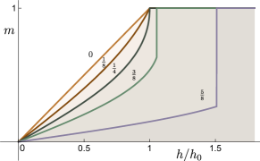
Figure 1: Saddle point result for the magnetization $m(h)$ for different values of interaction parameter $v$, which is shown next to each curve.

The saddle point of Eq. (2) with minimum action describes a cone (umbrella) state:

$$\hat{m}_{\rm sp}=(\varphi\cos qx,\varphi\sin qx,\sqrt{1-\varphi^{2}}),$$ (5)

with $0\leq\varphi\leq 1$ and $q$ functions of the parameters of the action. Solutions with both sign of $q$ are degenerate, which reflects spontaneous breaking of reflection symmetry and chiral order: $\hat{z}\cdot\hat{m}_{\rm sp}\times\partial_{x}\hat{m}_{\rm sp}=\varphi^{2}q\neq 0$. For sufficient large field, $h>h_{c}$, the solution is simply the ferromagnetic one, with $\varphi=0$. On reducing the field, there are two possible behaviors. For $\upsilon>-\kappa/4$ ($v<1/4$), a continuous transition occurs at the critical field $h_{c}=h_{0}=\delta^{2}/(2\kappa)$. The “order parameter” $\varphi$, which represents the local moment transverse to the magnetic field, increases smoothly from zero below $h_{0}$. This corresponds to the point of local instability of the FM phase to single magnons, which Bose condense when their energy vanishes at $h_{0}$. For $\upsilon<-\kappa/4$ ($v>1/4$), the transition occurs discontinuously at $h_{c}>h_{0}$, at which point the ferromagnetic state is still locally stable. The order parameter jumps to a non-zero value $\varphi_{c}$ for $h=h_{c}-0^{+}$. This is a metamagnetic transition, described by

$$\varphi_{c}^{2}=\frac{2\sqrt{v}-1}{v},h_{c}=\frac{\delta^{2}}{8\kappa\sqrt{v}(1-\sqrt{v})},q_{c}^{2}=\frac{\delta}{4\kappa(1-\sqrt{v})},$$ (6)

which hold for $1/4<v<1$. Due to the aforementioned scale invariance, the metamagnetic line extends for all $\delta$ at the saddle point level. We emphasize that the saddle point results are asymptotically exact, and hence provide direct predictions for experiment for systems close to the Lifshitz point. For example, the saddle-point behavior of the magnetization $m=\sqrt{1-\varphi^{2}}$ is shown in Fig. 1.

Quantum corrections: Fluctuations beyond the saddle point have several types of effects. One innocuous effect is that of phase fluctuations within the “cone phase”: configurations of form of Eq. (5) with $qx\rightarrow qx+\theta$ have small action when $\theta(x,\tau)$ has small space-time gradients. Fluctuations of $\theta$ are thereby described by a free boson theory with central charge $c=1$, which converts the long-range cone order into power-law spin correlations, but preserves the chiral order. These properties characterize a “vector chiral” phase (VC), identified previously in the FFHC.

A more drastic effect of fluctuations is to move the phase boundaries and even introduce new phases. This is due to the differing contribution of fluctuations to the ground state energy of different states. Quantum fluctuations modify the energy of the cone state but do not affect that of the (fluctuationless) ferromagnetic state. Hence fluctuations may shift the FM-cone transition to lower magnetic field. Remembering that $h_{0}$ is the single magnon condensation field, it makes sense to ask if quantum fluctuations can lower $h_{c}$ all way down to $h_{0}$? Note that affirmative answer to this question implies the appearance of the metamagnetic endpoint beyond which the FM-cone transition becomes continuous.

To investigate this question, we write the magnetization $\hat{m}$ in the co-moving system of coordinates

$$\hat{m}=\sqrt{2-\frac{\bar{\eta}\eta}{s}}[\frac{\bar{\eta}+\eta}{2\sqrt{s}}\hat{e}_{1}+i\frac{\bar{\eta}-\eta}{2\sqrt{s}}\hat{e}_{2}]+(1-\frac{\bar{\eta}\eta}{s})\hat{e}_{3},$$ (7)

where the rotating dreibein $\hat{e}_{j}(x)$ are chosen as follows: $\hat{e}_{1}\times\hat{e}_{2}=\hat{e}_{3}\equiv\hat{m}_{\rm sp}$. The fields $\bar{\eta},\eta$ describe magnons, transverse fluctuations of the magnetization. To quadratic order the action in Eq. (2) becomes $S=\int\!d\tau\left[\int dx\,\bar{\eta}\partial_{\tau}\eta+H_{\rm fluct}\right]$, which shows that $\bar{\eta},\eta$ are canonical Bose operators, and $H_{\rm fluc}(\bar{\eta},\eta)$ is a Hamiltonian. Fourier transforming it into momentum space shows that $H_{\rm fluc}$ contains both normal and anomalous terms:

$$H_{\rm fluc}=\sum_{k}2A_{k}\bar{\eta}_{k}\eta_{k}+B_{k}(\eta_{k}\eta_{-k}+\bar{\eta}_{k}\bar{\eta}_{-k}).$$ (8)

Here coefficients $A_{k},B_{k}$ are functions of momentum $k$ and depend on parameters $\delta,\kappa,v,h$ and $\varphi$ of the saddle point action. Diagonalization of (8) with the help of a standard Bogoluiubov transformation gives us the desired correction: the zero-point energy $\delta{\cal E}_{\rm cone}=\frac{1}{N}\sum_{k}\{\sqrt{A_{k}^{2}-B_{k}^{2}}-A_{k}\}$.

We use this corrected energy to identify a metamagnetic endpoint. A metamagnetic endpoint occurs at $\delta=\delta_{c}$ if, for $\delta>\delta_{c}$, the cone state remains higher in energy than the FM state for all $h\geq h_{0}$, while for $\delta<\delta_{c}$, the cone state has lower energy than the FM one for some range of fields $h_{0}<h<h_{c}$. Hence the endpoint is determined by the condition that the energy of the cone state equals that of the FM state at $h=h_{0}$, i.e. $\Delta E=\Delta{\cal E}-\delta{\cal E}_{\rm cone}=0$ at $h=h_{0}$ where the first term $\Delta{\cal E}={\cal E}_{FM}-{\cal E}_{\rm cone}$ represents the saddle point energy difference, and the last is the Bogoliubov correction.

Before analyzing this in detail, we note that from Eq. (4), the fluctuation corrections to the energy are expected to be reduced from the saddle point value by a factor of $\sqrt{\delta/\kappa}$, which is assumed small for consistency of the approach. Hence they can affect the balance between cone and FM states only when the energy difference between the two is already small at the saddle point level. Therefore we now focus on the regime close to the onset of metamagnetism, and let $v=1/4+\epsilon$ in what follows, with $\epsilon\ll 1$. In this limit, $\Delta{\cal E}(h_{0})=\frac{256}{27}\kappa\epsilon^{3}(\delta/\kappa)^{2}$.

The fluctuation correction $\delta{\cal E}_{\rm cone}$ contains a regular cutoff-dependent part and a singular universal term. The former may be absorbed into a renormalized coupling $v\rightarrow\tilde{v}$ and likewise $\epsilon$. The latter represents a physically distinct contribution to the cone state energy. For the lattice FFHC it was obtained previously in Krivnov and Ovchinnikov (1996). We obtain $\delta{\cal E}_{\rm cone}^{\rm sing}=s^{-1}\int_{-\infty}^{\infty}\frac{dk}{2\pi}\frac{100\delta^{3}\epsilon^{2}}{\kappa^{2}k^{2}+2\kappa\delta}=(25\sqrt{2}/s)\kappa\epsilon^{2}(\delta/\kappa)^{5/2}$.

Now combining the saddle point and corrections, we find that the total energy $\Delta E=\Delta{\cal E}(h_{0})-\delta{\cal E}_{\rm cone}^{\rm sing}$ is seen to change sign at $\delta_{c}\approx 0.07\kappa s^{2}\epsilon^{2}$, indeed indicating a metamagnetic endpoint. Since $\delta_{c}\ll 1$ with $\epsilon\ll 1$, this is within the regime of validity of the field theory.

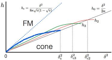
Figure 2: Stability curves (schematic). The thin dashed (blue) line shows the critical $h_{\rm c}$ field of the first order transition within the classical saddle point approximation. The wide brushed (blue) line indicates $h_{\rm c}$ as modified by quantum fluctuations. It crosses the thin (black) single-magnon instability field $h_{0}$ at $\delta=\delta_{c}$. The red (green) solid lines denote the critical magnetic fields $h_{2}(h_{3})$ describing two- (three-) magnon condensation instabilities. The $h_{3}(\delta)$ curve is a conjecture, see text for more details.

Quantum few-body physics: Considering the above result, we see that for $\delta>\delta_{c}$, the effective attraction between magnons is too weak to induce collapse. Hence one might conclude that the first instability of the ferromagnet upon reducing the field $h$ is to continuous single-magnon condensation at $h=h_{0}$. Here we argue this is incorrect, because there is a third possibility. While the attraction for $\delta>\delta_{c}$ is too weak to induce collapse, it still is strong enough to produce bound states of a finite number of magnons, which leads to distinct multipolar phases in a range $\delta_{c}<\delta<\delta_{c2}$, that set in at $h>h_{0}$.

As we consider larger $\delta$, the semiclassical analysis becomes inadequate, and a full quantum treatment of the action in Eq. (2) becomes necessary, which is daunting due to its non-polynomial nature (implicit in the NLsM constraint). In principle, by using Eq. (7) with $\hat{e}_{\mu}=\hat{x}_{\mu}$, one can expand and truncate the action to $\mathcal{O}(\eta^{2n})$ for an exact treatment of $n$-magnon states, since higher order terms, if properly normal-ordered, annihilate these states. This leads to a quantum Hamiltonian for bosonic fields $\overline{\eta},\eta$ with an unconventional kinetic energy and up to $n$-body momentum dependent interactions. Due to the complexity of this problem, we have limited ourselves to the $n=2$ case. This expansion yields

$$H = \sum_{k}\epsilon_{k}\overline{\eta}_{k}\eta_{k}$$

$$+\frac{1}{2L}\sum_{kpp^{\prime}}V(k,p,p^{\prime})\overline{\eta}_{k/2+p}\overline{\eta}_{k/2-p}\eta_{k/2-p^{\prime}}\eta_{k/2+p^{\prime}},$$

with $\epsilon_{k}=(h+2\kappa k^{4}-2\delta k^{2})/s$ and $V(k,p,p^{\prime})$ in sup .

One can gain some insight by focusing on the minima of $\epsilon_{k}$, which occur at $k=\pm q$, with $q=\sqrt{\delta/(2\kappa)}$. We therefore define new fields $\psi_{a,k}=\eta_{(2a-3)q+k}$ for $|k|\ll q$ and $a=1,2$. Then, Fourier transforming back to real space, one obtains, assuming all the scattered magnons remain near the two minima,

$$H = \int dx\,\Big{\{}\sum_{a=1}^{2}\overline{\psi}_{a}(\epsilon_{0}-\frac{\partial_{x}^{2}}{2m})\psi_{a}+$$

$$+\frac{1}{2}\gamma_{1}\left[(\overline{\psi}_{1}\psi_{1})^{2}+(\overline{\psi}_{2}\psi_{2})^{2}\right]+\gamma_{2}\overline{\psi}_{1}\psi_{1}\overline{\psi}_{2}\psi_{2}\Big{\}},$$

where $\epsilon_{0}=h/s-\delta^{2}/(2\kappa s)$, $m=s/8\delta$, $\qquad\gamma_{2}=\delta^{2}(5-4v)/(\kappa s^{2})$ and $\gamma_{1}=\delta^{2}(1-4v)/(2\kappa s^{2})$. Observe that for $v>1/4$, when the saddle point analysis found metamagnetism, the intra-valley interaction $\gamma_{1}$ is negative, i.e. attractive. As is well known, bosons with attractive delta-function potential, such as described by the $\gamma_{1}$ term in (A Panoply of Orders from a Quantum Lifshitz Field Theory), undergo collapse Calogero and Degasperis (1975); Kosevich et al. (1990); Krivnov and Ovchinnikov (1996) – the ground state of the system is given by the $N$-body bound state in which all $N$ bosons of the system participate. This collapse corresponds to the metamagnetic transition. In reality an infinite collapse is prevented by three-body interactions, and moreover the saddle point condition is renormalized with increasing $\delta$ as we found above, leading to the metamagnetic endpoint.

We can investigate renormalizations at the two-body level from Eq. (A Panoply of Orders from a Quantum Lifshitz Field Theory). In particular, taking the full dispersion and momentum-dependent interactions, we solve the two-body Schrödinger equation for the minimum energy state. The general form for such a state is $|\psi,k\rangle=\int\!\frac{dq}{2\pi}\Psi(q;k)\overline{\eta}_{k/2+q}\overline{\eta}_{k/2-q}|0\rangle$, where $|0\rangle$ is the boson vacuum, i.e. the ferromagnetic state, $k$ is the (conserved) center of mass momentum, and the two-magnon wavefunction obeys

$$(\epsilon_{k/2+p}+\epsilon_{k/2-p}-E)\Psi(p;k)+\int\!\frac{dp^{\prime}}{2\pi}V(k,p,p^{\prime})\Psi(p^{\prime};k)$$

$$=0.$$ (11)

This equation can be solved exactly sup . We obtain the minimum energy state for $k=\pm 2q$, which corresponds to a pair of magnons from the same minima, and find the binding energy $\epsilon_{b}=2\epsilon_{q}-E$ given by the relation

$$\sqrt{\epsilon_{b}}\approx\sqrt{\epsilon_{b0}}\left[1-\left(\frac{\delta}{\delta_{c2}}\right)^{1/2}\right]+\mathcal{O}(\delta^{5/2}),$$ (12)

where $\epsilon_{b0}=\epsilon^{2}\delta^{3}/(8\kappa^{2}s^{3})$ is just the naïve binding energy one would obtain from the delta-function interaction model, $\epsilon_{b0}=m\gamma_{1}^{2}/4$, and the term in the brackets represents the leading correction. This defines a critical value $\delta_{c2}=\frac{128}{625}\kappa s^{2}\epsilon^{2}\approx 0.2\kappa s^{2}\epsilon^{2}$, such that the two-magnon bound state disappears for $\delta>\delta_{c2}$.

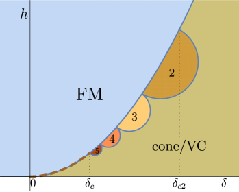
Figure 3: Schematic phase diagram in $\delta-h$ plane. The dashed line is the metamagnetic transition emerging from the Lifshitz point at the origin. “FM” and “cone/VC” denote the fully polarized ferromagnetic and cone/vector chiral phases, respectively. Integers $2,3,4,5$ label multipolar phases comprised of the corresponding number of bound magnons.

Importantly, we note that $\delta_{c2}>\delta_{c}$, which implies that in this interval the ferromagnetic state is unstable to two-magnon condensation for a non-zero range of fields $h>h_{0}$. In principle, we should now check for bound states of more than two magnons. Unfortunately, we have not been technically able to accomplish this. We speculate that in the range $\delta_{c}<\delta<\delta_{c2}$, bound states of increasing numbers of magnons appear with decreasing $\delta$, at thresholds $\delta_{c,n}$, with $\delta_{c}<\delta_{c,n}<\delta_{c,n^{\prime}}$ for $n>n^{\prime}$. This would imply a sequence of distinct multipolar phases just below saturation in this intermediate range of $\delta$, as shown schematically in Fig. 3. Note that the defining feature of the $n^{\rm th}$ multipolar phase is the presence of a gap for excitations with spin $S^{z}<n$. In one dimension, due to fluctuations, there is no true multipolar condensate, and each phase evolves smoothly from more condensate-like to spin-density-wave-like on reducing field Hikihara et al. (2008); Starykh and Balents (2014).

Microscopic calculation of $v$: The crucial dimensionless parameter $v$ of the theory cannot be determined within our field theory approach. We found two ways to fix its value by comparing field theory predictions with those of complimentary microscopic calculations sup . In the first, large spin $s\gg 1$ calculation, we use the standard spin-wave technique to calculate the leading spin-wave corrections to the ground state energy and the optimal spiral wave vector of the spin-$s$ $J_{1}-J_{2}$ chain. Comparing these results with the saddle point analysis, we find $v=3/(2s)$. Hence $v<1/4$ for large $s$, and thus metamagnetism occurs only for spin chains with $s<s_{c}=6$, in agreement with earlier Bethe-Salpeter calculations Arlego et al. (2011); Kolezhuk et al. (2012).

For the $s=1/2$ chain, we match the value of the order parameter jump $\varphi_{c}$, (6), at the metamagnetic transition to the corresponding value of the magnetization $m_{c}=(\sqrt{7}-1)/3$ reported in Ref. Krivnov and Ovchinnikov, 1996. This gives, via $m_{c}^{2}=1-\varphi_{c}^{2}$, that $v_{s=1/2}=1/(1+m_{c})^{2}\approx 0.42$. Given that $1/4<v_{s=1/2}<1$, our theory indeed predicts metamagnetism and multipolar phases for the FFHC, in agreement with numerical observations Sudan et al. (2009).

Generalizations and Outlook: The non-linear sigma model formulation can be easily extended to higher-dimensional Lifshitz points, and moreover, a rescaling argument similar to that in (4) continues to apply, implying that again asymptotically exact solutions are possible. This may provide a means to understand other frustrated ferromagnets and ferrimagnets, including possibly the kagomé lattice material volborthite Ishikawa et al. (2015); Janson et al. (2015), which shows signs of nematic-like behavior below an unusually-wide $1/3$ magnetization plateau.

Acknowledgements. We would like to thank A. Furusaki for detailed discussions of magnon binding. We also thank A. Chubukov, T. Momoi, Z. Hiroi and M. Takigawa for insightful discussions. Our work is supported by the NSF under grant no. DMR-15-06119 (L.B.) and DMR-12-06774 (O.A.S.). This research benefitted from the facility of the KITP, supported by NSF grant PHY11-25915.

Supplementary Information for “ A Panoply of Orders from a Quantum Lifshitz Field Theory”
Leon Balents and Oleg A. Starykh

I Saddle point analysis

The saddle point of Eq.2 with minimum action describes a cone (umbrella) state:

$$\hat{m}_{\rm sp}=(\varphi\cos qx,\varphi\sin qx,\sqrt{1-\varphi^{2}}).$$ (S-1)

The corresponding energy density is

$${\cal E}_{\rm cone}=-\delta\varphi^{2}+\kappa\varphi^{2}q^{4}-\kappa v\varphi^{4}q^{4}-h\sqrt{1-\varphi^{2}}.$$ (S-2)

Minimizing it over $q$ gives $q^{2}=\delta/(2\kappa(1-v\varphi^{2}))$. Hence

$${\cal E}_{\rm cone}=-\frac{\delta^{2}\varphi^{2}}{4\kappa(1-v\varphi^{2})}-h\sqrt{1-\varphi^{2}}.$$ (S-3)

Energy density of the ferromagnetic phase, where $\varphi=0$, is just ${\cal E}_{\rm FM}=-h$.

At the first order transition, two conditions should be satisfied: (a) ${\cal E}_{\rm cone}={\cal E}_{\rm FM}$, and (b) $\frac{\partial{\cal E}_{\rm cone}}{\partial\varphi^{2}}=0$. The first one tells that

$$b(1-\sqrt{1-\varphi^{2}})=\frac{\varphi^{2}}{2(1-v\varphi^{2})},$$ (S-4)

where $b=2\kappa h/\delta^{2}=h/h_{0}$, while the second leads to

$$b=\frac{\sqrt{1-\varphi^{2}}}{(1-v\varphi^{2})^{2}}.$$ (S-5)

Combining these two equations we find

$$\varphi_{c}^{2}=\frac{2\sqrt{v}-1}{v},h_{c}=\frac{\delta^{2}}{8\kappa\sqrt{v}(1-\sqrt{v})},~{}{\text{and}}~{}q_{c}^{2}=\frac{\delta}{4\kappa(1-\sqrt{v})}.$$ (S-6)

Observe that $h_{c}>h_{0}=\delta^{2}/(2\kappa)$ for $v>1/4$.

Condition (b) [Eq.(S-5)] applies everywhere inside the cone phase and is used to find the magnetization $m=\sqrt{1-\varphi^{2}}$. Namely, it leads to $b^{2}(1-v\varphi^{2})^{4}=(v-1)/v+(1-v\varphi^{2})/v$. In terms of $z=1-v\varphi^{2}$ this gives quartic equation $b^{2}z^{4}-z/v+(1-v)/v=0$, solution of which gives $z(b)$ for a given $v$. We find that there is only one physical root in the entire interval $0<v<1$. Differentiating both sides of (S-5) with respect to $b$ one finds relation between $m^{\prime}=\partial m/\partial b$ and the magnetization, $m^{\prime}=(1-v+vm^{2})^{3}/(1-v-3vm^{2})$. Hence, near $m=0$ the slope of the magnetization (that is, spin susceptibility) is $(1-v)^{2}/h_{0}$. Near the saturation, $m=1$, the slope is $1/(h_{0}(1-4v))$. In particular, at the critical $v=1/4$, separating the continuous from the discontinuous transitions, the slope diverges. For $v>1/4$ magnetization is continuous up to $m_{c}=\sqrt{1-\varphi_{c}^{2}}=(1-\sqrt{v})/\sqrt{v}$, which is reached at $h_{c}=h_{0}/(4\sqrt{v}(1-\sqrt{v}))>h_{0}$. It jumps to the saturation, $m_{\rm sat}=1$, at $h=h_{c}+0$. This behavior is easily identifiable in Fig.1 of the main text.

To find the cone state energy at $h=h_{0}$, which is required in our analysis of the metamagnetic endpoint, we need to solve Eq.(S-5) at $b=1$. Assuming that corresponding order parameter $\varphi_{0}$ is proportional to $\varphi_{c}$ at the critical point, $\varphi_{0}^{2}=a\varphi_{c}^{2}$, and expanding to second order in $\epsilon=v-1/4\ll 1$, we find $a=4/3$. It then easy to find that $\Delta{\cal E}(h_{0})={\cal E}_{FM}-{\cal E}_{\rm cone}|_{h_{0}}=256\epsilon^{3}\delta^{2}/(27\kappa)$.

II Metamagnetic endpoint

Magnon Hamiltonian

$$H_{\rm fluc}=\sum_{k}2A_{k}\bar{\eta}_{k}\eta_{k}+B_{k}(\eta_{k}\eta_{-k}+\bar{\eta}_{k}\bar{\eta}_{-k}).$$ (S-7)

leads to the zero-point energy $\delta{\cal E}_{\rm cone}=\int_{-\Lambda_{0}}^{\Lambda_{0}}\frac{dk}{2\pi}\{\sqrt{A_{k}^{2}-B_{k}^{2}}-A_{k}\}$.

We find that

$$sA_{k}=\kappa k^{4}+\frac{3-6v^{1/2}+6v-4v^{3/2}}{4v(1-v^{1/2})}k^{2}+\frac{(3-14v^{1/2}+20v-8v^{3/2})\delta^{2}}{32\kappa(1-v^{1/2})^{2}v}$$ (S-8)

and

$$sB_{k}=\frac{\delta(2v^{1/2}-1)}{32\kappa(1-v^{1/2})^{2}v}\Big{(}8\kappa(1-v^{1/2})(3-2v)k^{2}+(3-8v^{1/2}+4v)\delta\Big{)}$$ (S-9)

In the limit $v=1/4+\epsilon,\epsilon\to 0$ these simplify to

$$sA_{k} = \kappa k^{4}+2\delta k^{2}-10\delta k^{2}\epsilon+(38\delta k^{2}+\frac{4\delta^{2}}{\kappa})\epsilon^{2}+...$$

$$sB_{k} = 10\delta k^{2}\epsilon-(38\delta k^{2}+\frac{4\delta^{2}}{\kappa})\epsilon^{2}+...$$ (S-10)

Then, to the same $\epsilon^{2}$ accuracy,

$$\{\sqrt{A_{k}^{2}-B_{k}^{2}}-A_{k}\}\to-\frac{50\epsilon^{2}\delta^{2}k^{2}}{s(\kappa k^{2}+2\delta)}=-\frac{50\epsilon^{2}\delta^{2}}{s\kappa}+\frac{100\epsilon^{2}\delta^{2}}{s(\kappa k^{2}+2\delta)}$$ (S-11)

As a result

$$\delta{\cal E}_{\rm cone}=-\frac{50\epsilon^{2}\delta^{2}\Lambda_{0}}{s\kappa\pi}+\frac{25\sqrt{2}\epsilon^{2}\delta^{5/2}}{s\kappa^{3/2}},$$ (S-12)

where in the second term the integration was extended to infinity due to its convergence.

Observe that the first term represents a regular correction $\delta{\cal E}_{\rm cone}^{\rm reg}=-\frac{50\epsilon^{2}\delta^{2}\Lambda_{0}}{s\kappa\pi}$, which scales with $\delta$ the same way as the saddle-point energy $\Delta{\cal E}(h_{0})=\frac{256}{27}\frac{\epsilon^{3}\delta^{2}}{\kappa}$. It can be sought of as a renormalization of $\epsilon=v-1/4$ by quantum fluctuations.

The second term, on the other hand, is a singular $\delta{\cal E}_{\rm cone}^{\rm sing}=\frac{25\sqrt{2}\epsilon^{2}\delta^{5/2}}{s\kappa^{3/2}}$ correction which scales as fractional, ${5/2}$, power of $\delta$. It represents a physically distinct contribution to the cone state energy.

Thus, as described in the main text, $\Delta E=\Delta{\cal E}(h_{0})-\delta{\cal E}_{\rm cone}^{\rm sing}$ turns to zero at $\delta_{c}=(\frac{256}{25\cdot 27\sqrt{2}})^{2}\kappa s^{2}\epsilon^{2}\approx 0.07\kappa s^{2}\epsilon^{2}\ll 1$.

III Two-particle Schrodinger equation in the continuum

Using parameterization eq.7 with $(\hat{e}_{1},\hat{e}_{2},\hat{e}_{3})=(\hat{x},\hat{y},\hat{z})$, as appropriate for the fully polarized vacuum state, we find that action eq.2 turns into

$$S = \int dxd\tau~{}\bar{\eta}\partial_{\tau}\eta+\cal{H}_{\eta},$$

$${\cal H}_{\eta} = \frac{1}{s}\Big{(}h\bar{\eta}\eta-2\delta\bar{\eta}^{\prime}\eta^{\prime}+2\kappa\bar{\eta}^{\prime\prime}\eta^{\prime\prime}\Big{)}+\frac{1}{2s^{2}}\Big{(}-\delta[\bar{\eta}^{2}(\eta^{\prime})^{2}+(\bar{\eta}^{\prime})^{2}\eta^{2}]+8(1-v)\kappa(\bar{\eta}^{\prime})^{2}(\eta^{\prime})^{2}+$$ (S-13)

$$4\kappa[\eta\eta^{\prime}\bar{\eta}^{\prime}\bar{\eta}^{\prime\prime}+\bar{\eta}\bar{\eta}^{\prime}\eta^{\prime}\eta^{\prime\prime}]-2\kappa[\bar{\eta}\bar{\eta}^{\prime\prime}(\eta^{\prime})^{2}+\eta\eta^{\prime\prime}(\bar{\eta}^{\prime})^{2}]+\kappa[\bar{\eta}^{2}(\eta^{\prime\prime})^{2}+\eta^{2}(\bar{\eta}^{\prime\prime})^{2}]\Big{)},$$

where prime stands for spatial derivative.

Fourier transforming gives

$$H=\sum_{k}\epsilon_{k}\overline{\eta}_{k}\eta_{k}+\frac{1}{2L}\sum_{kpp^{\prime}}V(k,p,p^{\prime})\overline{\eta}_{k/2+p}\overline{\eta}_{k/2-p}\eta_{k/2-p^{\prime}}\eta_{k/2+p^{\prime}},$$

with $\epsilon_{k}=(h+2\kappa k^{4}-2\delta k^{2})/s$ and the symmetrized potential $V(k,p,q)$ is given by

$$V(k,p,q) = \frac{1}{s^{2}}\Big{\{}\frac{1}{2}\delta k^{2}-\frac{1}{8}\kappa(1+4v)k^{4}-\delta(p^{2}+q^{2})+$$ (S-14)

$$+\kappa\Big{(}p^{4}+q^{4}+\frac{1}{2}(-3+4v)k^{2}(p^{2}+q^{2})+4(3-2v)p^{2}q^{2}\Big{)}\Big{\}}$$

Observe that as far as the spin $s$ dependence goes, $V(k,p,q)$ is actually $s$-independent, as it should be, because both $\delta$ and $\kappa$ scale as $s^{2}$. Observe also that the center of mass (CM) momentum of the pair $k$ couples to the relative momenta $p$ and $q$. In our case $k=2q_{0}=\sqrt{2\delta/\kappa}$. Assuming for the moment that $p,q\ll q_{0}$, we can extract the constant (momentum-independent) part of the interaction

$$V(2q_{0},0,0)=\frac{2\kappa(1-4v)q_{0}^{4}}{s^{2}}=\frac{(1-4v)\delta^{2}}{2\kappa s^{2}}=\gamma_{1}.$$ (S-15)

This is just $\gamma_{1}$, an attractive contact interaction (for $v>1/4$) between magnons from the same valley.

The general form of a two-particle state is $|\psi,k\rangle=\int\!\frac{dq}{2\pi}\Psi(q;k)\overline{\eta}_{k/2+q}\overline{\eta}_{k/2-q}|0\rangle$, where $|0\rangle$ is the boson vacuum, i.e. the ferromagnetic state, $k$ is the (conserved) center of mass momentum, and the two-magnon wavefunction obeys

$$(\epsilon_{k/2+p}+\epsilon_{k/2-p}-E)\Psi(p;k)+\int\!\frac{dq}{2\pi}V(k,p,q)\Psi(q;k)=0.$$ (S-16)

The minimum energy state for $k=2q_{0}$ is parameterized in terms of the bound state energy $\epsilon_{b}$ measured from the minimum of two-particle continuum at $k=2q_{0}$ as $E=(2h-4\kappa q_{0}^{4})/s-\epsilon_{b}$. Then (A Panoply of Orders from a Quantum Lifshitz Field Theory)

$$\Big{(}s\epsilon_{b}+16\kappa q_{0}^{2}p^{2}+4\kappa p^{4}\Big{)}\Psi(p;2q_{0})=-s\int\frac{dq}{2\pi}V(2q_{0},p,q)\Psi(q;2q_{0})$$

$$=-s\int\frac{dq}{2\pi}\Big{(}\gamma_{1}-\frac{8\kappa q_{0}^{2}(1-v)}{s^{2}}(p^{2}+q^{2})+\frac{4\kappa(3-2v)}{s^{2}}p^{2}q^{2}+\frac{\kappa}{s^{2}}(p^{4}+q^{4})\Big{)}\Psi(q;2q_{0})$$ (S-17)

In the very simple limit of $p,q\ll q_{0}$, which corresponds to the low-energy Hamiltonian eq.10, we are allowed to neglect all momentum dependent terms in the integrand of the right-hand-side. Then

$$\int\frac{dp}{2\pi}\Psi(p;2q_{0})=\int\frac{dp}{2\pi}\frac{-s\gamma_{1}}{s\epsilon_{b}+16\kappa q_{0}^{2}p^{2}}\int\frac{dq}{2\pi}\Psi(q;2q_{0})$$ (S-18)

which leads, for $\gamma_{1}<0$, to the bound state energy $\epsilon_{b0}=\kappa(1-4v)^{2}q_{0}^{6}/(16s^{3})=(1-4v)^{2}\delta^{3}/(128s^{3}\kappa^{2})=\epsilon^{2}\delta^{3}/(8s^{3}\kappa^{2})$. (Remember that $v=1/4+\epsilon$.) This, of course, describes the bound state due to an attractive delta-function potential of strength $\gamma_{1}$.

The solution of the full equation (12) is more complicated. We first turn it into a linear algebra problem $\psi_{n}=\sum_{m=0,2,4}A_{n,m}\psi_{m}$ for the moments $\psi_{n}=\int_{-\Lambda_{0}}^{\Lambda_{0}}\frac{dq}{2\pi}q^{n}\Psi(q;2q_{0})$. The bound state energy $\epsilon_{b}$ is then found from ${\text{det}}[A-\hat{1}]=0$. Note that the matrix elements of $A$ are formed by momentum integrals involving upto 8th power of momentum in the numerator and 4th power of momentum in the denominator of the integrand. This requires special care in treating divergent integrals. The upper cut-off $\Lambda_{0}$ is such that $q_{0}\ll\Lambda_{0}\ll 1$. The first (left) inequality allows us to account for inter-valley scattering with momentum transfer of the order $\pm 2q_{0}$, while the second (right) follows from the fact that the field theory is formulated in continuum and is obtained by integrating out all lattice-scale fluctuations with wave vectors of order $1$ (the lattice spacing is set to 1 for convenience). We proceed by carefully treating converging ($\Lambda_{0}$-independent) elements of $A$ and by separating singular (in $\epsilon_{b}\to 0$ limit) elements there from order 1 contributions. The rest of matrix elements is organized in power series in $\Lambda_{0}\ll 1$. Plugging these all back in ${\text{det}}[A-\hat{1}]=0$ we finally obtain

$$\sqrt{\epsilon_{b}}\approx\sqrt{\epsilon_{b0}}\left[1-\left(\frac{\delta}{\delta_{c2}}\right)^{1/2}\right]+\mathcal{O}(\delta^{5/2}),$$ (S-19)

Here $\delta_{c2}=128\kappa s^{2}\epsilon^{2}/625$, and $\epsilon_{b0}$ is actually written in terms of the renormalized interaction parameter $\tilde{\epsilon}=\epsilon+25\Lambda_{0}/(8\pi s)$. The bound state disappears for $\delta>\delta_{c2}$.

IV Parameters of the action

To find bare values of $\delta,\kappa$ and $\upsilon$ for the action $S$ (Eq.2 of the main text), we match, at $h=0$, single-particle dispersion as predicted by the field theory $\epsilon_{k}=(2\kappa k^{4}-2\delta k^{2})/s$ (see eq.9 and discussion below it) with that obtained directly from the lattice FFHC model, in the limit of small momentum $k$. The latter one is given by $\omega_{k}=2s(J_{1}(\cos[k]-1)+J_{2}(\cos[2k]-1))\to 2s((\frac{1}{2}-2\beta)k^{2}+(\frac{2\beta}{3}-\frac{1}{24})k^{4})$, where we set $J_{1}=-1$ and $J_{2}=\beta$. Hence $\delta=s^{2}(4\beta-1)/2$ and $\kappa=s^{2}(\frac{2\beta}{3}-\frac{1}{24})\to s^{2}/8$, where we set $\beta=1/4$ in the expression for $\kappa$. Note that $\upsilon=0$ at this classical, $s^{2}$, level.

The saddle point analysis. Using that $\varphi=0$ at $h=0$ and $\hat{m}=(\cos qx,\sin qx,0)$ we find ${\cal E}_{\rm cone}(q)=-\delta q^{2}+\kappa q^{4}+\upsilon(q^{2})^{2}$. Clearly, the optimal $q$ is $q_{\rm sp}^{2}=\delta/(2(\kappa+\upsilon))$ and ${\cal E}_{\rm cone}(q_{\rm sp})=-\delta^{2}/(4(\kappa+\upsilon))$. Hence, we can turn these relations around as $\delta=-2{\cal E}_{\rm cone}(q_{\rm sp})/q_{\rm sp}^{2}$ and $\kappa+\upsilon=-{\cal E}_{\rm cone}(q_{\rm sp})/q_{\rm sp}^{4}$. (Observe that ${\cal E}_{\rm fm}=0$.)

Then, using the result $q=q_{0}(1+\frac{3}{4s})$ of the large-$s$ calculation described in the next Section IV.1, we obtain

$$\delta=\frac{2s^{2}}{q_{0}^{2}(1+\frac{3}{4s})^{2}}\frac{(J_{1}+4J_{2})^{2}}{8J_{2}}(1+\frac{3}{2s})=s^{2}(2\beta-1/2)+O(s^{0}),$$ (S-20)

which means that $\delta$ is not changed by quantum fluctuations to our $1/s$ order.

Similarly, for $\kappa+\upsilon$ we get

$$\kappa+\upsilon=\frac{2s^{2}}{q_{0}^{4}(1+\frac{3}{4s})^{4}}\frac{(J_{1}+4J_{2})^{2}}{8J_{2}}(1+\frac{3}{2s})=s^{2}(\frac{J_{2}}{2}-\frac{3J_{2}}{4s})+O(s^{0})),$$ (S-21)

Assuming that $\kappa=s^{2}J_{2}/2=s^{2}/8$ does not renormalize (because, at $\delta=0$, it describes excitations of the state with no quantum fluctuations), we see that $\upsilon=-3J_{2}s/4=-3s/16$ and hence $v=-\upsilon/\kappa=3/(2s)$.

Thus,

$$\delta=\frac{s^{2}(4\beta-1)}{2},\kappa=\frac{s^{2}}{8},\upsilon=-\frac{3s}{16},v=\frac{3}{2s}.$$ (S-22)

IV.1 Large-$s$ calculation of $v$

Our goal is to determine the quantum fluctuation term $\upsilon$ in the NLsM by comparing the wavevector of the exact ground state to that predicted by the NLsM. Of course we do not know the exact wavevector, but at least we can obtain the $1/s$ correction to the classical one. In this section, we discuss how to obtain such a $1/s$ correction to $q$.

The idea is to calculate the energy as a function of the ordering wavevector $q$, and minimize it. A priori we expect that the energy density $e(q)$ has a series expansion,

$$e(q)=s^{2}e_{0}(q)+se_{1}(q)+\cdots$$ (S-23)

To minimize it, we require $e^{\prime}(q)=0$. We then let

$$q=q_{0}+\frac{1}{s}q_{1}+\cdots$$ (S-24)

We can collect the terms to the first two orders, which give the conditions

$$e^{\prime}_{0}(q_{0}) = 0,$$ (S-25)

$$e^{\prime\prime}_{0}(q_{0})q_{1}+e^{\prime}_{1}(q_{0}) = 0.$$ (S-26)

The first condition just expresses that $q_{0}$ is the classical minimum, and the second determines the leading correction $q_{1}$, which is what we are after.

The Hamiltonian

$$H=\sum_{n}J_{1}\vec{S}_{n}\cdot\vec{S}_{n+1}+J_{2}\vec{S}_{n}\cdot\vec{S}_{n+2}$$ (S-27)

is studied by transforming into rotating grame

$$\left(\begin{array}[]{c}S^{x}_{n}\\ S^{y}_{n}\\ S^{z}_{n}\end{array}\right)=\left(\begin{array}[]{ccc}\cos qn&-\sin qn&0\\ \sin qn&\cos qn&0\\ 0&0&1\end{array}\right)\left(\begin{array}[]{c}S^{1}_{n}\\ S^{2}_{n}\\ S^{3}_{n}\end{array}\right)$$ (S-37)

and expanding spin in the local basis as

$$\left(\begin{array}[]{c}S^{1}_{n}\\ S^{2}_{n}\\ S^{3}_{n}\end{array}\right)=\left(\begin{array}[]{c}S-a^{\dagger}_{n}a_{n}\\ \sqrt{\frac{S}{2}}(a^{\dagger}_{n}+a_{n})\\ i\sqrt{\frac{S}{2}}(a^{\dagger}_{n}-a_{n})\end{array}\right).$$ (S-44)

This gives for the classical energy per spin

$$e_{0}(q)=J_{1}\cos q+J_{2}\cos 2q,$$ (S-45)

minimization of which leads, of course, to $\cos q_{0}=-J_{1}/(4J_{2})$, so that $q_{0}\approx\sqrt{8(\beta-1/4)}$. The energy of the ferromagnetic state, $q=0$, is $e_{0;fm}=J_{1}+J_{2}$.

Leading quantum fluctuations are described by

$$H^{(2)}=S\sum_{k}\{2A_{k}a^{\dagger}_{k}a_{k}-B_{k}(a_{k}a_{-k}+a^{\dagger}_{k}a^{\dagger}_{-k})\}$$ (S-46)

with

$$2A_{k} = J_{1}[(1+\cos q)\cos k-2\cos q]+J_{2}[(1+\cos 2q)\cos 2k-2\cos 2q],$$

$$2B_{k} = J_{1}(1-\cos q)\cos k+J_{2}(1-\cos 2q)\cos 2k.$$ (S-47)

Note that in the ferromagnetic state $q=0$ the anomalous part is absent, $B_{k}=0$.

Diagonalizing $H^{(2)}$ we find the required zero-point motion energy

$$e_{1}(q)=\frac{1}{N}\sum_{k}(\Omega_{k}-A_{k})=J_{1}\cos q+J_{2}\cos 2q+\frac{1}{N}\sum_{k}\Omega_{k},$$ (S-48)

where $\Omega_{k}=\sqrt{A_{k}^{2}-B_{k}^{2}}$. As a result, we need to calculate $e_{1}^{\prime}(q_{0})=\frac{1}{N}\sum_{k}\frac{\partial\Omega_{k}}{\partial q}|_{J_{1}=-4J_{2}\cos q_{0}}$. That is, take derivative of $\Omega_{k}$ over $q$, and then make the substitution $J_{1}=-4J_{2}\cos q_{0}$. The obtained result can then be expanded in powers of $q_{0}\ll 1$ (which is well justified near the Lifshitz point) to the 3rd order and integrated over $k$. In this way we find $e_{1}^{\prime}(q_{0})=-3J_{2}q_{0}^{3}$ and $q_{1}=3q_{0}/4$, so that $q=q_{0}(1+\frac{3}{4s})$.

Observe that by virtue of the relation $\delta\sim q_{0}^{2}$, this result implies the scaling $e_{1}\sim q_{0}^{4}\sim\delta^{2}$. However, calculation of the higher order in $\delta$ terms, of the type $\delta^{n}$ with $n\geq 3$, results in infrared divergent integrals. These divergencies imply that the whole perturbation series needs to be re-summed in order to obtain a finite $\delta^{5/2}$ contribution found in the main text. Luckily, large-$s$ calculation of the interaction parameter $v$ does not require these higher powers of $\delta$.

To summarize, large-$s$ calculation predicts $q=q_{0}(1+\frac{3}{4s})$ and cone state energy, relative to that of the ferromagnetic state, $e(q)=s^{2}(e_{0}-e_{0;fm})+se_{1}=-s^{2}\frac{(J_{1}+4J_{2})^{2}}{8J_{2}}(1+\frac{3}{2s})$.

References

Andreev and Grishchuk (1984)
A. F. Andreev and
I. A. Grishchuk,
JETP 60, 267
(1984).
Zhitomirsky and Tsunetsugu (2010)
M. E. Zhitomirsky
and
H. Tsunetsugu,
EPL (Europhysics Letters) 92,
37001 (2010).
Svistov et al. (2011)
L. Svistov,
T. Fujita,
H. Yamaguchi,
S. Kimura,
K. Omura,
A. Prokofiev,
A. Smirnov,
Z. Honda, and
M. Hagiwara,
JETP Letters 93,
21 (2011), ISSN 0021-3640,
URL http://dx.doi.org/10.1134/S0021364011010073.
Masuda et al. (2011)
T. Masuda,
M. Hagihala,
Y. Kondoh,
K. Kaneko, and
N. Metoki,
Journal of the Physical Society of Japan
80, 113705
(2011), eprint http://dx.doi.org/10.1143/JPSJ.80.113705,
URL http://dx.doi.org/10.1143/JPSJ.80.113705.
Mourigal et al. (2012)
M. Mourigal,
M. Enderle,
B. Fåk,
R. K. Kremer,
J. M. Law,
A. Schneidewind,
A. Hiess, and
A. Prokofiev,
Phys. Rev. Lett. 109,
027203 (2012).
Nawa et al. (2013)
K. Nawa,
M. Takigawa,
M. Yoshida, and
K. Yoshimura,
Journal of the Physical Society of Japan
82, 094709
(2013), eprint http://dx.doi.org/10.7566/JPSJ.82.094709,
URL http://dx.doi.org/10.7566/JPSJ.82.094709.
Nawa et al. (2014)
K. Nawa,
Y. Okamoto,
A. Matsuo,
K. Kindo,
Y. Kitahara,
S. Yoshida,
S. Ikeda,
S. Hara,
T. Sakurai,
S. Okubo,
et al., Journal of the Physical Society of
Japan 83, 103702
(2014), eprint http://dx.doi.org/10.7566/JPSJ.83.103702,
URL http://dx.doi.org/10.7566/JPSJ.83.103702.
Prozorova et al. (2015)
L. A. Prozorova,
S. S. Sosin,
L. E. Svistov,
N. Büttgen,
J. B. Kemper,
A. P. Reyes,
S. Riggs,
A. Prokofiev,
and O. A.
Petrenko, Phys. Rev. B
91, 174410
(2015),
URL http://link.aps.org/doi/10.1103/PhysRevB.91.174410.
Willenberg et al. (2015)
B. Willenberg,
M. Schäpers,
A. U. B. Wolter,
S.-L. Drechsler,
M. Reehuis,
B. Büchner,
A. J. Studer,
K. C. Rule,
B. Ouladdiaf,
S. Süllow,
et al., ArXiv e-prints
(2015), eprint 1508.02207.
Kolezhuk (2002)
A. K. Kolezhuk,
Progress of Theoretical Physics Supplement
145, 29 (2002),
eprint http://ptps.oxfordjournals.org/content/145/29.full.pdf+html,
URL http://ptps.oxfordjournals.org/content/145/29.abstract.
Sirker et al. (2011)
J. Sirker,
V. Y. Krivnov,
D. V. Dmitriev,
A. Herzog,
O. Janson,
S. Nishimoto,
S.-L. Drechsler,
and J. Richter,
Phys. Rev. B 84,
144403 (2011),
URL http://link.aps.org/doi/10.1103/PhysRevB.84.144403.
Ishikawa et al. (2015)
H. Ishikawa,
M. Yoshida,
K. Nawa,
M. Jeong,
S. Krämer,
M. Horvatić, C. Berthier,
M. Takigawa,
M. Akaki,
A. Miyake,
et al., Phys. Rev. Lett.
114, 227202
(2015),
URL http://link.aps.org/doi/10.1103/PhysRevLett.114.227202.
Janson et al. (2015)
O. Janson,
S. Furukawa,
T. Momoi,
P. Sindzingre,
J. Richter,
and K. Held,
ArXiv e-prints (2015),
eprint 1509.07333.