ASPCAP: the APOGEE Stellar Parameter and Chemical Abundances Pipeline

Abstract

The Apache Point Observatory Galactic Evolution Experiment (APOGEE) has built the largest moderately high-resolution ($R\approx 22,500$) spectroscopic map of the stars across the Milky Way, and including dust-obscured areas. The APOGEE Stellar Parameter and Chemical Abundances Pipeline (ASPCAP) is the software developed for the automated analysis of these spectra. ASPCAP determines atmospheric parameters and chemical abundances from observed spectra by comparing observed spectra to libraries of theoretical spectra, using $\chi^{2}$ minimization in a multidimensional parameter space. The package consists of a fortran90 code that does the actual minimization and a wrapper IDL code for book-keeping and data handling. This paper explains in detail the ASPCAP components and functionality, and presents results from a number of tests designed to check its performance. ASPCAP provides stellar effective temperatures, surface gravities, and metallicities precise to 2%, 0.1 dex, and 0.05 dex, respectively, for most APOGEE stars, which are predominantly giants. It also provides abundances for up to 15 chemical elements with various levels of precision, typically under 0.1 dex. The final data release (DR12) of the Sloan Digital Sky Survey III contains an APOGEE database of more than 150,000 stars. ASPCAP development continues in the SDSS-IV APOGEE-2 survey.

1. Introduction

The Apache Point Observatory Galactic Evolution Experiment (APOGEE, Majewski et al. 2015) is one of the three projects of the Sloan Digital Sky Survey III (SDSS-III; Eisenstein et al., 2011). Between 2011-2014, the survey obtained high-resolution, near infrared (IR) spectra of over $150,000$ stars using the APOGEE multi-object spectrograph (Wilson et al., 2012) attached to the Sloan 2.5-m telescope (Gunn et al., 2006). Observations will continue through 2020 in the framework of the APOGEE-2 survey, part of SDSS-IV. The three main Galactic stellar components (bulge, disk, and halo) are mapped using the kinematical and chemical information derived from an automated spectral analysis. The unparalleled APOGEE stellar sample and associated data products represent a powerful means to understand the origins and evolution of the Milky Way.

APOGEE targeted red giant stars selected from the 2MASS Point Source Catalog (Skrutskie et al., 2006), employing de-reddened photometry and a simple color cut ($7\leq H\leq 13.8$ and $[J-K]_{0}\geq 0.5$; for more details, see Zasowski et al. 2013). The majority of targets have effective temperatures in the range 3500 $<T_{\rm eff}<5500$ K, although warmer (telluric) stars were also targeted to correct for absorption lines produced in the atmosphere of the Earth (H₂O, CO₂, and CH₄). About $20\%$ of the stars in APOGEE are dwarfs.

APOGEE performs a detailed characterization of the inner Galaxy via the near-infrared observation of a large numbers of stars and the accompanying derivation of their kinematical and chemical properties at high precision. The $H$-band (1.51-1.70 ${\mu}$m) APOGEE observations are acquired at high resolution ($R=22,500$) and high signal-to-noise ($S/N\geq$ 100 per half-resolution element or $\sim$ per pixel). They are also rich in chemical information. At least 15 individual element abundances can be measured, and the $S/N$ ratio is high enough to allow typical abundance precisions better than 0.1 dex. Such multi-dimensional study requires an automated, detailed, and accurate spectral analysis pipeline. This level of automated analysis would be challenging under any circumstances, and it is particularly challenging for the $H$-band wavelength regime, where many features are blended (e.g., by molecular line contaminants) and which has not been studied as extensively as optical ranges.

Several optical surveys have already created automated spectral analysis software used for the extraction of atmospheric parameters and chemical abundances, including: the Sloan Extension for Galactic Understanding and Exploration (SEGUE; Yanny et al., 2009), the Radial Velocity Experiment (RAVE; e.g, Steinmetz et al., 2006), the Large Sky Area Multi-Object Fiber Spectroscopic Telescope (LAMOST) Experiment for Galactic Understanding and Exploration,(LEGUE; Zhao et al., 2012), the Abundances and Radial Velocity Galactic Origins Survey (ARGOS; Freeman et al., 2013), and the Gaia-ESO Survey (GES; Gilmore et al., 2012). Notably, SEGUE (Lee et al., 2008) and LEGUE (Xiang et al., 2015) generate data products through fully-automated, completely self-contained analysis “pipelines” (named the SEGUE Stellar Parameter Pipeline [SSPP] and the LAMOST Stellar Parameter Pipeline [LASP]).

APOGEE has developed its own pipeline for parameter determinations: the APOGEE Stellar Parameter and Chemical Abundances Pipeline (ASPCAP). This pipeline operates on combined visit or individual-visit spectra processed by the APOGEE data reduction pipeline (Nidever et al., 2015). ASPCAP is innovative in the use of the $H$-band to extract abundances accurately for a large number of elements (up to 15) in an immense stellar sample ($>10^{5}$ targets). ASPCAP performs spectral analysis over a wide wavelength range ($\sim 200$ nm) and consequently, manipulates a large volume of data (approximately $10^{4}$ wavelength points). Further complicating the analysis is the presence in typical APOGEE targets of numerous molecular features (from CO, CN and OH lines) that can affect the determination of the spectroscopic parameters via the contribution of these features to the molecular equilibrium and continuous opacity.

The first year of APOGEE observations and ASPCAP results were released in the Sloan Digital Sky Survey $10^{\mathrm{th}}$ data release (DR10; Ahn et al. 2014), while the full (three years) APOGEE database of more than 150,000 stars is now publicly available in DR12 (Alam et al. 2015). The APOGEE reduction and analysis software is also released through the SDSS repository.

This paper provides a thorough description of the ASPCAP software as well as relays the results of numerous performance and reliability tests. Section 2 presents the overall structure of the ASPCAP software. In Section 3, the model spectra employed in the ASPCAP analysis of APOGEE data are discussed. Sections 4 and 5 contain detailed descriptions of the $\chi^{2}$ minimization code ferre and the IDL wrapper, respectively. Section 6 is devoted to the testing of the ASPCAP algorithms and the software. Finally, Section 7 reviews the performance of the ASPCAP pipeline with actual APOGEE Survey data.

2. Overall ASPCAP Structure

The ASPCAP software has two main functional components: a fortran90 code (ferre, Section 4), and an IDL wrapper (Section 5). The general schematic of ASPCAP is displayed in Figure 1. The IDL wrapper is multifunctional in that it reads the input APOGEE spectra and prepares them for analysis as well as performs the overall “bookkeeping”, which entails multiple calls to the fortran90 optimization code. The workhorse of ASPCAP is the fortran90 code, which compares the APOGEE observed spectra to a library of synthetic spectra and, subsequently, identifies the set of atmospheric parameters and abundances that yields the best fit spectrum. Specifically, during the observed spectrum fitting process, the fortran90 code performs an interpolation in the synthetic spectral grid and generates a best-fit (interpolated) synthetic spectrum, which then allows for the final parameter extraction.

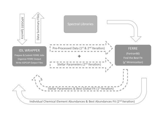
Figure 1.— Overview of ASPCAP workflow. The IDL wrapper pre-processes the APOGEE spectra for FERRE, which identifies the best six- or seven-parameter fit (depending on whether microturbulence is free or fixed), using the model spectral libraries. On the second iteration, FERRE is run fitting one elemental abundance at a time, with windows used to select the portions of the spectrum that are sensitive to that element. The IDL wrapper writes output files based on the FERRE results.

As shown in Figure 1, the iterative determination of ASPCAP proceeds in a two-step fashion. The first step is to assign the input APOGEE observed spectrum a set of fundamental atmospheric parameters (effective temperature, $T_{\rm{eff}}$; surface gravity, $\log{g}$; microturbulent velocity, $\xi_{\rm{t}}$; scaled-solar general metallicity, [M/H]) from a first-pass fit of the entire APOGEE spectrum. In conjunction with these parameters, the abundances of C, N and the $\alpha$-elements (O, Mg, Si, S, Ca, and Ti) are also allowed to vary around the scaled-solar values due to their significant spectral contribution in the $H$-band. Figure 2 gives an illustration of an (example) APOGEE spectrum for a cool, solar metallicity giant and its best ASPCAP global fit. The second step of ASPCAP is to extract the individual element abundances, one at a time, from the fitting of spectral windows. These windows have been optimized for each element.

3. Model Spectra

The model synthetic spectra are generated by solving the radiative transfer equation for a grid of model atmospheres over the APOGEE portion of the $H$-band wavelength regime. In this section we provide details on the model atmospheres, the atomic and molecular line lists, and the spectral synthesis calculations. Some information on the structure of the ASPCAP databases is also provided.

3.1. Model Atmospheres

ASPCAP uses a set of model atmospheres specifically generated for APOGEE; the APOGEE ATLAS9 models (Mészáros et al., 2012), which are based on the ATLAS9 model atmosphere code from Castelli & Kurucz (2004). These models are one-dimensional, assume local themodynamic equilibrium (LTE), and use no convective overshooting. In DR10, ASPCAP results relied upon on ATLAS9 models with scaled-solar compositions and the set of solar reference photospheric abundances from Grevesse & Sauval (1998). For DR12, the results were based upon customized abundances (a set of varied C, N, and $\alpha$ contents at a given metallicity) and a more recent set of solar reference abundances (Asplund et al. 2005, the photospheric abundance column of their Table 1). The grid steps for the atmospheric parameters and (C, N, $\alpha$) abundances as well as the associated ranges are given in Table 1 (see Zamora et al. 2015 for library names nomenclature). Note that the step sizes are small enough to minimize interpolation uncertainties and also allow for efficient ASPCAP computation and performance.

3.2. Line List

The input atomic and molecular data are essential for accurate determination of the atmospheric parameters and abundances. The base line list originated from the R. Kurucz website (http://kurucz.harvard.edu/), which provides wavelengths, excitation potentials, oscillator strengths, and hyperfine structure information. Best effort was then made to update line list values with laboratory measurements of wavelength and (most critically) oscillator strengths. When possible, van der Waals damping constants based on the study of Barklem, Anstee, & O’Mara (1998) were used. Molecular data for CO, OH, CN, C₂, H₂ and SiH were included. Finally, astrophysical inversion from matching the spectra of the Sun and Arcturus ($\alpha$ Boo) was employed to fine tune line list values (i.e., gf’s and C6 constants). For a complete description of the line list assembly, consult Shetrone et al. (2015). The final line list adopted for DR10 was m201105101120 and for DR12, m201312161124.

3.3. Spectral Synthesis

The synthetic spectral library was generated with the line transfer code ASS$\epsilon$T (Koesterke, 2009; Koesterke et al., 2008). The solar photospheric reference abundances from Asplund et al. (2005) were adopted and a terrestrial isotopic composition for C, N, and O was used. Initially, synthetic spectra were computed at very high spectral resolution (1–2 km s^-1) and then, later re-smoothed to account for instrumental broadening. Three spectral regions, which correspond to the spectral coverage of the three APOGEE detectors, are synthesized: $\lambda=$1.51681–1.57923 ${\mu}$m, 1.58814–1.64166 ${\mu}$m, and 1.64995–1.69367 ${\mu}$m (vacuum wavelengths). The resampling of the synthetic spectra to match that of the APOGEE observed spectra was done with a constant step size in $\log{\lambda}$—see Table 2. In that table, $N_{\mathrm{pixels}}$ and $p_{i}$ are the number of pixels and the pixel ith number for each detector synthesized spectrum, respectively. Additional details regarding the available synthetic spectral libraries can be found in Zamora et al. (2015).

The spectra in DR10 were convolved with a Gaussian kernel to bring the resolving power $\lambda/$FWHM$\equiv~{}R=22,500$. For DR12, the convolution employed a more realistic, empirical kernel (Holtzman et al. 2015, Nidever et al. 2015). For the APOGEE instrumental set-up, spectral resolution variations as high as 10–15% can occur for different fibers as well as across the APOGEE wavelength regime. In DR12, accounting for some of these LSF variations (Nidever et al., 2015) was done by averaging the LSF’s of five fibers that were located at equidistant steps along the pseudoslit and then fitting them with a Gauss-Hermite function that varied with wavelength. The impact of LSF treatment is discussed in §6.5. DR10 ignored macroturbulence, which is usually significantly smaller than the instrumental broadening. However, DR12 used a constant value of 6 km s^-1(FWHM) for the macroturbulence, modeled with a Gaussian kernel. Note that neither DR10 nor DR12 considered rotational broadening, which could compromise the quality of the derived ASPCAP values for fast rotating stars.

Table 1Synthetic Spectra Libraries

Name	$T_{\rm{eff}}$			$\log{g}$			[M/H]			[C/M]			[N/M]			[$\alpha$/M]			Data Release
										Low High Step
p_aps23k0821_w123	3500	5000	250	0	5	0.5	$-2.5$	+0.5	0.5	$-1$	+1	0.25	$-1$	+1	0.5	$-1$	+1	0.25	DR10
p_aps23k0921_w123	4750	6000	250	0	5	0.5	$-2.5$	+0.5	0.5	$-1$	+1	0.25	$-1$	+1	0.5	$-1$	+1	0.25	DR10
n_aps23k2121_w123	6000	10000	1000	2	5	1.0	$-2.5$	+0.5	0.5	+0	+0	0.00	+0	+0	0.0	+0	+0	0.00	DR10
n_aps23k3121_w123	8000	15000	1000	3	5	1.0	$-1.0$	+0.0	1.0	+0	+0	0.00	+0	+0	0.0	+0	+0	0.00	DR10
p6_apsasGK_131216_lsfcombo5v6	3500	6000	250	0	5	0.5	$-2.5$	+0.5	0.5	$-1$	$+1$	0.25	$-1$	$+1$	0.5	$-1$	$+1$	0.25	DR12
p6_apsasF_131216_lsfcombo5v6	5500	8000	250	1	5	0.5	$-2.5$	+0.5	0.5	$-1$	$+1$	0.25	$-1$	$+1$	0.5	$-1$	$+1$	0.25	DR12

Table 2Library wavelength scale ($\log\lambda=\mathrm{a}_{0}+\mathrm{a}_{1}*p_{i}$)

Npixels	a0	a1
2920	4.180932	6.000000E-06
2400	4.200888	6.000000E-06
1894	4.217472	6.000000E-06

3.4. Principal Component Analysis Compression

The cool-star libraries used in ASPCAP have typical sizes of tens of gigabytes. There are 5–11 nodes per dimension, 6 or 7 dimensions (3 dimensions for hot stars) per library, and of order 10⁴ wavelengths. Accessing the libraries on a hard drive, as a direct-access file, is much slower than holding them in RAM, but even when they do fit in the computer’s RAM, accessing the data becomes slower as the arrays grow in size.

Reducing the size of libraries has many advantages, and we achieve that by applying principal component analysis compression (PCA; Pearson 1901) to identify correlations between the fluxes at different wavelengths and compress the model spectra.

The full arrays are too large to perform PCA on them. We split the arrays into several dozen contiguous wavelength intervals (30 pieces with $\sim 300$ wavelengths each) and run PCA on those. We retain the first 30 components for each, creating arrays of PCA coefficients that are the concatenation of the coefficients for each wavelength interval (900 coefficients in total). This procedure is very effective, reducing the size of the libraries by nearly a factor of ten. Compression is done on the library nodes independently of ASPCAP runs. The analysis of simulations with PCA libraries works well at the metallicities typical of APOGEE targets but can cause some problems at low metallicities—see Section 6.2.

3.5. Database Preparation

ASPCAP searches in grids of pre-computed, normalized, convolved, and PCA-compressed synthetic spectra that cover the stellar spectral classes from early-M to F in DR12 (3500–8000 K), and to B (3500–15000 K) in DR10—see Table 1. There are separate grids per spectral class. ASPCAP analysis is not optimized for early-type stars, thus they are not analyzed in DR12. The parameter space searched includes the atmospheric stellar parameters $T_{\rm{eff}}$, $\log{g}$, and [M/H], and, in most cases, the C, N, and $\alpha$-element abundances. Molecular features are used to derive the C, N, and O abundances, but these features disappear in the spectra of hot stars. In the DR10 analysis of stars hotter than 6000 K, the number of searched parameters was reduced by requiring solar scaled abundances, [$\alpha$/M]$=$[C/M]$=$[N/M]$=0$.

In principle, atmospheric microturbulence is an additional parameter to be considered in the fitting of the APOGEE spectra, however we found it more effective to reduce the dimensionality of the problem by adopting a linear relationship between microturbulence and surface gravity:

$$\begin{split}\xi_{\rm t}&=2.240-0.300\log g\quad{\rm(DR10)}\\ \xi_{\rm t}&=2.478-0.325\log g\quad{\rm(DR12)},\end{split}$$ (1)

and a $\xi_{\rm{t}}$$\ =2$ km s^-1 in the DR10 analysis of stars hotter than 6000 K. The $\xi_{\rm{t}}$-$\log{g}$ relations were derived using a subsample of the APOGEE data analyzed with a library in which the microturbulence is a free parameter.

4. FERRE

ferre is the optimization code that finds the parameters of the model spectrum that best matches an observed spectrum. The code is written in fortran90 and can take advantage of multi-core processors, performing optimizations for several spectra in parallel using OpenMP. ferre has been applied to a number of data sets before APOGEE (e.g., SDSS SEGUE and BOSS, as illustrated in Allende Prieto et al. 2006, 2014). ferre can be used with different configurations that allow a choice of different search algorithms or interpolation schemes, which are chosen in a control file.

4.1. Algorithm

Observed spectra are matched against a grid of synthetic spectra to search for the best fit. The search algorithms compare observations and model spectra using the $\chi^{2}$ as a merit function

$$\chi^{2}=\sum_{\lambda}\frac{(O_{\lambda}-F_{\lambda})^{2}}{\sigma_{\lambda}^{2}},$$ (2)

where $O_{\lambda}$ are the observed fluxes, $F_{\lambda}$ the model fluxes, and $1/\sigma_{\lambda}^{2}$ the weights.

The weights are calculated directly from the error bars for the fluxes computed during data reduction, increasing artificially the uncertainties in regions severely affected by sky emission lines. When deriving abundances, the $\chi^{2}$ merit function also takes into account the sensitivity of different spectral features to changes in the abundance of the elements of interest, the lack of sensitivity to other elements, and the level of agreement between model spectra and actual APOGEE observations as a function of wavelength—see Section 4.3.

Searches are initialized at specific locations. Currently for the global parameter fit, we are working with 12 searches, which are symmetrically distributed over the parameter space, at the centers of the 6D cells resulting from dividing the ranges in [C/M], [N/M], and [$\alpha$/M] in one bin, the ranges in [M/H] and $\log{g}$ in two bins, and the range $T_{\rm{eff}}$ in three bins. The optimization is carried out using the Nelder & Mead (1965) algorithm, which evaluates and compares the $\chi^{2}$ at the test points of the simplex (a triangle in multi-dimensions). As search continues, the simplex moves to a series of rules, which can shift the search off the nodes of the grid in an attempt to reach regions where the chi-squared is lower. The algorithm typically requires a few hundred evaluations of the $\chi^{2}$ for a 6D search in our cool-star databases. The search stops when the convergence criterion is satisfied: a standard deviation below $10^{-4}$ for the values of $\chi^{2}$ evaluated at the test points of the simplex. There is no special treatment in ferre for dealing with a flat $\chi^{2}$ surface, e.g., for the cases of non-detection of a spectral feature in abundance determinations. The minimization that yields the lowest $\chi^{2}$ among the 12 searches is accepted as the best fit.

Model fluxes need to be interpolated to evaluate fluxes at points off the grid nodes; the interpolation in fluxes is more accurate than interpolations of atmospheric structures (Mészáros & Allende Prieto, 2013). Early APOGEE ASPCAP analyses and interpolation tests (see Section 6.1) give more accurate results for higher polynomial orders. ASPCAP used cubic Bèzier interpolation for both DR10 and DR12. Solving for abundances from the global fit with linear or quadratic interpolation leads to solutions that systematically cluster the results around the spectral library nodes. This effect is more significant for spectra with $S/N<50$, and while this effect becomes very small at $S/N>70$, smaller steps when implemented in the grid (0.25 dex instead of 0.5 dex for [C/M] and [$\alpha$/M]) help to minimize the problem.

ferre has an option to use masks to block spectral windows, or more generally to use weights that depend on wavelength in the $\chi^{2}$ evaluation. ASPCAP uses this capability to ignore bad and/or contaminated pixels in the fitting process and in the determination of individual elemental abundances.

4.2. Errors

The internal random errors in the retrieved parameters can be estimated from the inverse of the curvature matrix. This was the method used in DR10 and DR12, and typically used in ferre. DR10 assumed these internal errors with a factor of 15 enhancement. The matrix elements of the curvature matrix ($\beta_{ij}$) are calculated from the partial derivatives of the synthetic spectra ($F_{\lambda}$):

$$\beta_{ij}=\sum_{\lambda}\frac{1}{\sigma_{\lambda}^{2}}\frac{\partial F_{\lambda}}{\partial P_{i}}\frac{\partial F_{\lambda}}{\partial P_{j}},$$ (3)

where $P_{i}$ are the different parameters/abundances considered in the optimization (Press et al., 2007) and $\sigma_{\lambda}$ the flux error. The inverse of the curvature matrix gives the parameter errors and their covariance under the assumption that the likelihood of the data is described by $\chi^{2}$ (${\cal L}\propto e^{-\chi^{2}/2})$ and that the model gives a correct description of the data (up to observational errors) for some choice of its parameters. ferre can also estimate errors by searching for the parameter solution multiple times after adding random noise to the observed spectra, according to the uncertainty in the observations. As discussed in §6.3, tests on synthetic spectra show that these two methods give comparable error estimates and that they reasonably capture the uncertainty associated with observational noise. However, empirical estimates of abundance uncertainties based on star clusters indicate that the true abundance errors are larger than these internal ASPCAP estimates (Holtzman et al., 2015), probably because (unsurprisingly) the model atmospheres and synthetic spectra remain an imperfect representation of the true spectra (see §6.3 for further discussion).

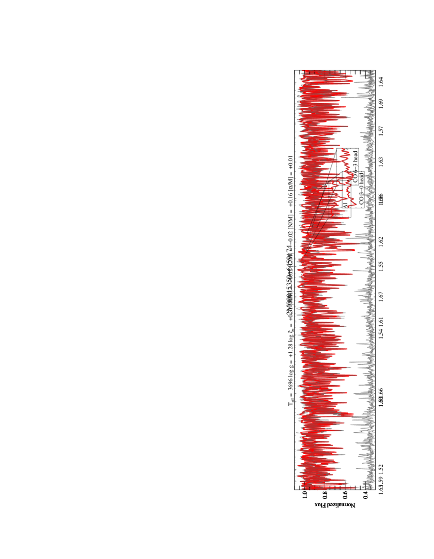
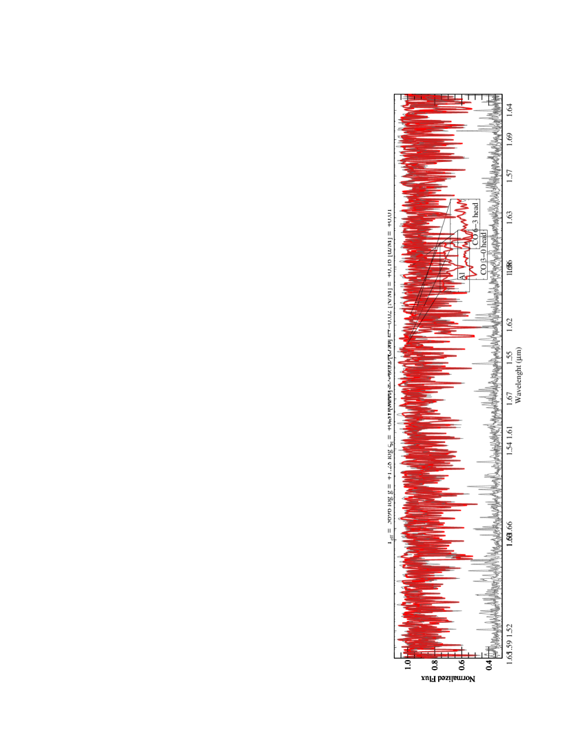
Figure 2.— The observed normalized spectrum (black) of the cool, solar metallicity star 2M00015350-6459174 ([M/H]$\ =-0.02$), its ASPCAP best spectral fit (red), and the residuals (relative differences), shifted by 0.35, are shown at the bottom of each panel. The spectrum from each of APOGEE’s three detectors is shown in a separate panel.

4.3. Derivation of Elemental Abundances

After the first ferre pass to derive atmospheric parameters from the entire APOGEE spectrum, we perform a series of new runs in which all parameters but that of the dimension used for the abundance of the element of interest remain fixed. Only specific spectral windows are fitted—see Figure 3. In these fittings, the same databases of synthetic spectra are used, but the abundances of individual $\alpha$-elements are derived by varying the [$\alpha$/M] dimension of the grid, the abundance of carbon and nitrogen by varying the [C/M] and [N/M] dimensions, respectively, and the abundances of all other elements by varying the [M/H] dimension. The weights for the $\chi^{2}$ calculations are also changed so that we only consider spectral features that are sensitive to the element of interest.

Deriving the relevant pixel weights for each element is equivalent to identifying the transitions to be used for each element. This is accomplished by first using an algorithm that evaluates the derivatives of the model fluxes with respect to each elemental abundance for a star with $T_{\rm{eff}}$$\ =4000$ K, $\log{g}$$\ =1.0$, and three different metallicities ([M/H]$\ =+0.0,-1.0,$ and $-2.0$). Wavelengths are assumed to be sensitive to abundance changes of a given element for each metallicity, if the modulus of the derivative is larger than three times the standard deviation of all points in the spectrum. Weights are normalized to the value of the most sensitive point. Therefore the weight at $\lambda$ for element $i$ at a metallicity [M/H] is proportional to the change of the flux with the abundance at that wavelength:

$$w^{\prime}_{\lambda,i,\mathrm{[M/H]}}\propto\frac{\partial F_{\lambda,\mathrm{[M/H]}}}{\partial A_{i}}.$$ (4)

If a wavelength is sensitive to the abundance of another element except for Fe, the weight of this other element is subtracted. This procedure can yield negative values, which are fixed to zero.

$$w_{\lambda,i,\mathrm{[M/H]}}=w^{\prime}_{\lambda,i,\rm{[M/H]}}-\sum\limits_{j\neq i,Fe}w^{\prime}_{\lambda,j,\mathrm{[M/H]}}.$$ (5)

All the weights obtained for each metallicity are combined in the form

$$\begin{split}w_{\lambda,i}=0.3\times w_{\lambda,i,\mathrm{[M/H]}=+0.0}\\ +0.3\times w_{\lambda,i,\mathrm{[M/H]}=-1.0}\\ +0.4\times w_{\lambda,i,\mathrm{[M/H]}=-2.0}.\end{split}$$ (6)

This favors those wavelengths that at low metallicity are sensitive to abundance changes, since significant variations of the modulus of the derivative are more difficult to detect in that metallicity regime. Weights are adjusted with a multiplicative factor $\alpha_{\lambda}$ that takes into account how well the model spectrum for Arcturus reproduces an actual (Hinkle et al. 1995) observation of this star. This multiplicative factor goes from one, when the ratio between model spectrum and atlas is lower than three times the sigma of the distribution, to zero for the most deviant points. A second multiplicative factor $\beta_{\lambda}$, takes into account how well APOGEE spectra are reproduced by the model fluxes, using the median residuals at each wavelength after fitting the entire APOGEE sample. Therefore the final weight for each element is in the form:

$$W_{\lambda,i}=\alpha_{\lambda}\times\beta_{\lambda}\times w_{\lambda,i}.$$ (7)

The whole procedure makes it possible to use only parts of a line profile, e.g., the red and/or blue wings, when the core is removed owing to any criteria described above (mostly blends) . Finally, a few regions were removed after a visual inspection of the fits for each element in the set of reference stars defined by Smith et al. (2013).

Table 3, available electronically, gives the weights as a function of wavelength, for the 15 APOGEE chemical elements. In the short portion of Table 3 shown in the text, only K has non-zero weight. The number of features used in the abundance determinations varies from element to element: there are dozens for C (mainly CO and CN), N (CN), O (OH), and Fe but only a handful for Na, Mg, Al, Si, S, K, Ca, Ti, V, Mn, and Ni. Most of the features are neutral versions of elements. Figure 3 shows the location of the spectral windows for each of the elements.

Table 3ASPCAP Spectral Windows for Chemical Abundances Determinations

Wavelength	Abundance Weights
	Fe	C	N	0	Na	Mg	Al	Si	S	K	Ca	Ti	V	Mn	Ni
($\mu$m)
1.516812988281	0.0000	0.0000	0.0000	0.0000	0.0000	0.0000	0.0000	0.0000	0.0000	0.0143	0.0000	0.0000	0.0000	0.0000	0.0000
1.516834667969	0.0000	0.0000	0.0000	0.0000	0.0000	0.0000	0.0000	0.0000	0.0000	0.0008	0.0000	0.0000	0.0000	0.0000	0.0000
1.516854687500	0.0000	0.0000	0.0000	0.0000	0.0000	0.0000	0.0000	0.0000	0.0000	0.0000	0.0000	0.0000	0.0000	0.0000	0.0000
1.516876269531	0.0000	0.0000	0.0000	0.0000	0.0000	0.0000	0.0000	0.0000	0.0000	0.0000	0.0000	0.0000	0.0000	0.0000	0.0000
1.516896289062	0.0000	0.0000	0.0000	0.0000	0.0000	0.0000	0.0000	0.0000	0.0000	0.0000	0.0000	0.0000	0.0000	0.0000	0.0000

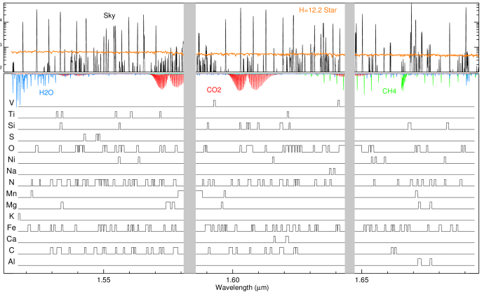
Figure 3.— The ASPCAP spectral windows for the 15 APOGEE chemical elements along with examples of APOGEE sky (black), telluric (blue, red and green), and stellar spectra (orange). To aid visibility, the spectral windows are broadened by $\pm 30$ km s^-1, and all weights are set to the same value. Full information is available in electronic Table 3.

5. IDL wrapper

While ferre performs the search for the optimal set of parameters for each observed spectrum, there are many other tasks that need to be done before and after the optimization. A suite of IDL programs called the IDL Wrapper performs those other tasks.

The wrapper works in blocks of observations defined by fields. APOGEE fields are typically defined by their Galactic coordinates ($l,b$) or their location ID ($locID$, a unique four digit number assigned to each APOGEE field). The reading of the data is done separately for each individual field, and the pre-processing and analysis runs are done independently for each individual stellar spectral class.

5.1. Data Preparation

Observations are compared to synthetic spectra in the stellar rest frame. The data reduction pipeline corrects the observed wavelengths for Doppler shifts associated with the stellar radial velocities estimated by the pipeline itself, and using a sinc interpolation places the observed spectra in the wavelength scale of the synthesis (for more details, see Nidever et al., 2015).

The comparison of observations to synthetic spectra uses continuum-normalized fluxes to minimize differences associated with reddening and the instrumental response function. The normalization of the observed and synthetic spectra should be the same to minimize systematic differences. In the case of individual abundances derivations, ASPCAP employs the normalized observed spectra used for the global fit.

We have opted for a simple normalization procedure, based on a pseudo rather than a real continuum, to facilitate consistency with observations. The normalization consists of a repeated least-squares polynomial fit ($O_{\lambda,\mathrm{fit}}=\Sigma a_{i}*\lambda^{i}$) after successive sigma clippings. Each APOGEE detector spectrum is normalized independently, as done for the library spectra. The library continuum information is stored in the library header and used by ASPCAP. The parameters of the fit are: the polynomial order, the number of iterations, and the rejection levels, which are given in units of the standard deviation between the previous polynomial fit and the retained data. ASPCAP uses a fourth-order polynomial and ten iterations. The algorithm looks for the spectrum’s upper envelope, which is reached by employing small lower ($0.1\times\sigma$) and moderate upper ($3.0\times\sigma$) clipping thresholds. The first iteration fits the spectrum and replaces the rejected pixels with the fitted values.

Observations can suffer from systematic errors and depart from the synthetic spectra. These errors may be associated with minor typical instrument defects, the instrumental response, or the contribution of the Earth’s atmosphere and the interstellar medium. A good instrument characterization provides information on detector cosmetics (bad and/or saturated pixels), which can be used to avoid problematic pixels. The continuum fitting process and the $\chi^{2}$ evaluation ignore bad pixels and those affected by cosmic rays. The data reduction pipeline produces flux-calibrated spectra from which sky emission has been subtracted and telluric absorption has been removed, along with uncertainties for the spectra. However, the sky subtraction is imperfect, especially for the bright OH lines, so the uncertainties in regions around such lines are inflated so that they are effectively masked out. Early ASPCAP analyses of some APOGEE data showed little sensitivity of the parameter derivations to the masking of few spectral windows. The chosen windows simulated those potentially affected by sky emission contamination.

5.2. Jobs Management and Data Organization

The wrapper takes care of writing the ferre input files, submitting the ferre jobs to the execution queue, organizing the output, setting quality flags, and doing calibrations (see Holtzman et al., 2015, for more details on flags and calibration).

Output results are packed into FITS files (Pence et al., 2010), with a structure that resembles that of the files containing APOGEE spectra. The spectra themselves are included in output ASPCAP files (aspcapStar files). These spectra are exactly as input to ferre but they differ from those in the apStar files in two respects: they have been continuum normalized (see Section 5.1), and their spectral range is slightly reduced to ensure the same spectral lines are used in the analysis of all stars, regardless of their radial velocities. The best-fitting model spectra are also included in the files. The calculated parameters, abundances and their covariance matrices can be found in the allStar summary files.

Table 4Tests on Synthetic Spectra with Different ASPCAP Settings

Descrip.	Test	[M/H]		[C/M]		[N/M]		[$\alpha$/M]		$\log{\xi_{\rm{t}}}$		$T_{\rm{eff}}$		$\log{g}$
		${\Delta}$	$\sigma$	${\Delta}$	$\sigma$	${\Delta}$	$\sigma$	${\Delta}$	$\sigma$	${\Delta}$	$\sigma$	${\Delta}$	$\sigma$	${\Delta}$	$\sigma$
		(dex)		(dex)		(dex)		(dex)		(dex)		(K)		(dex)
On-nodes sample
Linear Interpolation	A	$+0.000$	$0.004$	$+0.000$	$0.020$	$+0.000$	$0.275$	$+0.000$	$0.006$	$+0.001$	$0.015$	$+0.015$	$10.414$	$+0.000$	$0.021$
Quadratic Interpolation		$-0.000$	$0.002$	$-0.000$	$0.006$	$+0.000$	$0.187$	$+0.000$	$0.002$	$+0.001$	$0.005$	$+0.016$	$4.005$	$+0.000$	$0.008$
		$+0.000$	$0.003$	$+0.000$	$0.013$	$-0.000$	$0.313$	$+0.000$	$0.003$	$+0.001$	$0.013$	$+0.028$	$7.382$	$+0.000$	$0.016$Results listed are for the sample in common with that used in Test A, cubic interpolation case.
Cubic Interpolation		$+0.000$	$0.002$	$+0.000$	$0.010$	$+0.000$	$0.309$	$+0.000$	$0.002$	$+0.001$	$0.008$	$+0.028$	$5.706$	$+0.000$	$0.011$
Linear with PCA	B	$-0.003$	$0.051$	$+0.000$	$0.202$	$+0.044$	$0.440$	$+0.007$	$0.048$	$+0.006$	$0.115$	$+7.542$	$69.880$	$+0.012$	$0.146$
Quadratic with PCA		$+0.001$	$0.051$	$+0.009$	$0.196$	$+0.085$	$0.452$	$+0.006$	$0.050$	$+0.005$	$0.110$	$+7.735$	$69.958$	$+0.016$	$0.148$
Cubic with PCA		$-0.000$	$0.050$	$+0.009$	$0.196$	$+0.087$	$0.454$	$+0.006$	$0.051$	$+0.005$	$0.108$	$+7.233$	$68.366$	$+0.015$	$0.144$
[M/H]$>-1$ & $T_{\rm{eff}}$$<5500$		$+0.002$	$0.028$	$+0.002$	$0.100$	$+0.029$	$0.233$	$+0.004$	$0.038$	$+0.004$	$0.033$	$+5.045$	$51.641$	$+0.010$	$0.106$
Off-nodes sample
$S/N=\inf$	C	$-0.002$	$0.013$	$-0.009$	$0.039$	$+0.019$	$0.173$	$-0.000$	$0.011$	$-0.002$	$0.024$	$-0.700$	$20.950$	$-0.000$	$0.031$
$S/N$=25		$+0.035$	$0.045$	$-0.018$	$0.095$	$+0.072$	$0.276$	$-0.002$	$0.037$	$-0.002$	$0.065$	$+13.400$	$61.650$	$+0.003$	$0.090$
$S/N$=50		$+0.006$	$0.022$	$-0.010$	$0.060$	$+0.028$	$0.200$	$-0.001$	$0.022$	$-0.002$	$0.036$	$+2.400$	$31.500$	$+0.001$	$0.053$
$S/N$=100		$-0.001$	$0.016$	$-0.010$	$0.045$	$+0.021$	$0.168$	$-0.001$	$0.015$	$-0.003$	$0.029$	$+0.000$	$23.250$	$+0.000$	$0.037$
$S/N$=200		$-0.002$	$0.015$	$-0.007$	$0.041$	$+0.024$	$0.188$	$-0.000$	$0.012$	$-0.002$	$0.025$	$-0.800$	$21.600$	$+0.000$	$0.033$
Blocking	D	$-0.002$	$0.016$	$-0.010$	$0.045$	$+0.022$	$0.196$	$-0.000$	$0.014$	$-0.004$	$0.030$	$-0.700$	$22.750$	$-0.001$	$0.036$
Reduced on-nodes sample
Ref.	E	$+0.000$	$0.017$	$+0.002$	$0.042$	$+0.021$	$0.201$	$+0.002$	$0.015$	$-0.000$	$0.048$	$+2.600$	$17.700$	$+0.008$	$0.036$
Lower Res.		$+0.021$	$0.033$	$-0.003$	$0.076$	$+0.029$	$0.246$	$+0.009$	$0.021$	$+0.020$	$0.101$	$-15.800$	$43.800$	$-0.082$	$0.099$
DR12 LSF		$+0.024$	$0.032$	$-0.014$	$0.055$	$+0.041$	$0.211$	$+0.013$	$0.030$	$+0.034$	$0.095$	$-14.300$	$40.050$	$-0.088$	$0.093$

6. Tests on simulated data

The performance of ASPCAP is, naturally, dependent on stellar properties. For reference, Figure 4 plots the distribution of DR12 stars in $T_{\rm{eff}}$ versus [M/H]. Only stars on the main survey with reliable parameters are shown; i.e., stars with neither of the bits set in the EXTRATARG bitmaks and with no BAD_STAR bit set in the ASPCAPFLAG bitmask). While APOGEE stars span a wide range of $T_{\rm{eff}}$ and [M/H] parameters, the great majority of good main survey stars (83%) lie in the range $-0.7\leq{\rm[M/H]}\leq 0.2$ and $3500\,{\rm K}\leq T_{\rm eff}\leq 5100\,{\rm K}$.

We evaluate the performance of our analysis methodology using two sets of simulated data and a 7D analysis (i.e., with microturbulence as a free parameter). First we use the very same model spectra in one of our libraries as simulated observations, to check whether there are degeneracies among the many parameters involved in our analysis, and to test the effect of using PCA compression. We carry out these tests using linear, quadratic, and cubic interpolation in the grid of model spectra during the search. Second, we use a sample of model spectra computed for parameters off the grid nodes. These are created in the same way as the grid synthetic spectra, computing model atmospheres and spectra for the parameters. This data set is used to quantify the impact in the ASPCAP parameter results of interpolation errors, noise in the spectra, and the effect of the information removal or degradation caused by sky lines or telluric absorption.

The first data set includes 17,640 spectra extracted from a library with the same synthetic spectra used in the cool library ($3500\leq T_{\rm eff}\leq 6000$ K) for DR12, but smoothed to a resolving power of R$=22,500$ with a Gaussian kernel. Since the spectra will be analyzed with the same library from which they come, the details of the broadening function do not matter. The parameters for this “on-nodes” data set are uniformly distributed in the parameter space, leaving out the boundaries of the grid, where the search algorithm runs into problems. In some tests, we used a subset of these spectra to reduce the computing time (“reduced on-nodes sample”), with 194 spectra sampled uniformly from the larger sample. The second data set (“off-nodes sample”) is made of 1,000 synthesized spectra with randomly distributed parameter values and less extreme abundances (more typical of the APOGEE sample)—e.g., Figure 4.

The on-nodes sample covers $3750\leq$ $T_{\rm{eff}}$ (K) $\leq 5750$, $0.5\leq$ $\log{g}$ (cgs) $\leq 4.5$, $-2.0\leq$ [M/H] $\leq 0.0$, $-0.75\leq\$[C/M] and [$\alpha$/M]$\ \leq$ 0.75, $-0.5\leq[\rm{N/Fe}]\leq 0.5$ and $0.0\leq\log{\xi_{\rm{t}}}$ (km s^-1) $\leq 0.6$. The reduced on-nodes subset has a similar coverage but sparser sampling. The coverage of the off-nodes sample is restricted to a single value for the microturbulence, 2 km s^-1, and $4000\leq$ $T_{\rm{eff}}$(K) $\leq 6000$, $0.5\leq$ $\log{g}$(cgs) $\leq 5.0$, $-2.0\leq$[M/H] $\leq 0.5$ , and $-0.5\leq\$[X/M]$\ \leq 0.5$ for [C/M], [N/M], and [$\alpha$/M]. We quantify the results of our tests by comparing the true parameters of the test spectra with those recovered by ferre in terms of median offsets ($\Delta$) in Table 4. We use a robust measure of the dispersion in the offsets ($\sigma$) to avoid outliers: we calculate the difference between the maximum and the minimum offsets after excluding the largest 15.85% of the sample and the smallest 15.85%, and divide it by two, which would correspond to the standard deviation in a normal distribution. The values of the dispersion we find in the different tests are in general larger than the values we would find by fitting a Gaussian curve to the distributions, but lower than a straight calculation of the standard deviation, and we think they are a more solid metric to compare the results from different tests. These are the figures we report as $\sigma$ in Table 4.

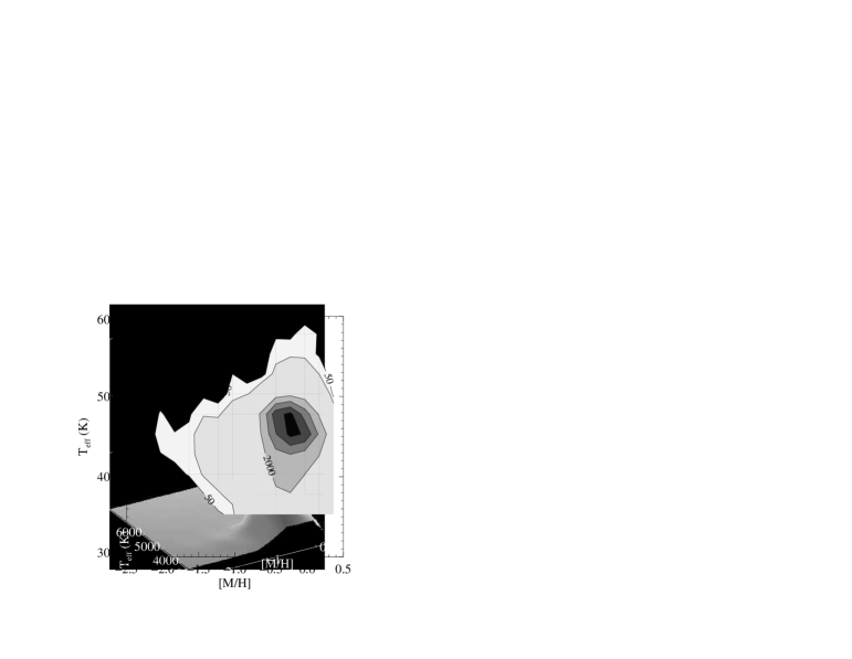
Figure 4.— The number of DR12 stars (not flagged as bad) in the $T_{\rm{eff}}$-[M/H] plane, using ASPCAP parameter values without calibration corrections. The contour lines are for levels of 50, 100, 2000, 4000, 6000, and 8000 stars.

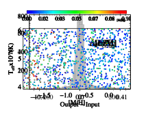
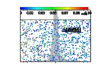
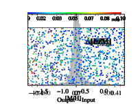
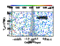
Figure 5.— Histograms of the differences (output$\ -\$input) for the seven global fit parameters for the off-node synthetic spectra with $S/N$=100.

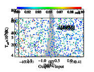
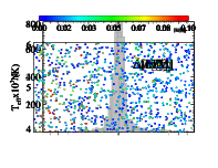
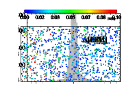
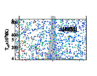
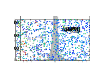
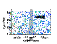
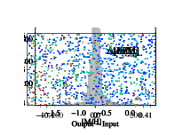
Figure 6.— The distribution of the input data in the $T_{\rm{eff}}$-[M/H] plane for the test with off-node synthetic spectra of $S/N$=100. Data are colored according to their parameter uncertainties, with each parameter displayed in a different panel. Data with larger differences than the maximum value of the color bar are scaled to that maximum value.

Our tests with cubic interpolation produced the best overall results. At the typical APOGEE metallicities ([M/H]$\ \gtrsim-1.0$), the stellar parameters and the abundances of C, N, and $\alpha$-elements were well recovered, even in the tests with PCA. Of some concern is the compression at lower metallicities, especially for C and N. The introduction of noise in the tests, at the level of $S/N=100$ per pixel, did not compromise the quality of the results. The surface gravity and the microturbulent velocity showed sensitivity to the LSF adopted, hence a detailed characterization of the LSF was done in DR12. We present below the results of our tests in more detail.

6.1. Test A. Order of Interpolations

As described above, ferre searches for the model parameters that best match the APOGEE data, and the evaluation of the model spectra as a function of stellar parameters is performed by interpolation in a pre-computed grid. We evaluated the performance of different interpolation schemes available in the code (linear, and Bèzier quadratic and cubic polynomials) in Mészáros & Allende Prieto (2013); currently ferre uses the same order for all the parameters. Here we test the effect of each scheme in the 7D analysis of the on-nodes sample. Of course, the result of a model spectrum evaluation occurring on a node is exact (to numerical round-off), independent of the interpolation scheme, but the convergence of the search method (the Nelder-Mead algorithm) will be affected by the accuracy of the model spectrum evaluation off the nodes at each step in the search process.

Our results are presented in Table 4 as case A for linear, quadratic, and cubic interpolation. The cubic test was performed in a slightly smaller sample to speed-up the analysis. For comparison purposes, results of the quadratic test for that sub-sample are also listed in Table 4. In the three interpolation cases we recover the input parameter values of the simulations well. The best performance is quadratic and cubic interpolation, for which the dispersion is about two times lower for most parameters than for the linear case. ASPCAP uses cubic interpolation for also reducing uncertainties associated with the clustering of solutions around the nodes of the spectral libraries. All the tests show small $\sigma$ values for most parameters. Nitrogen is the exception, with a [N/M] dispersion of 0.2–0.3 dex, as a result of the weakness of the CN bands in metal-poor spectra and the weak response of the CN lines to changes in the N abundance. For cubic interpolation, the dispersion of differences is $\leq 0.01$ dex for $\log{g}$, the other abundance parameters, and $\xi_{\rm t}$, and $6\,{\rm K}$ for $T_{\rm{eff}}$.

6.2. Test B. PCA Compression on the Nodes

ASPCAP uses PCA-compressed libraries to reduce execution time and memory requirements. Tests show that the derivation of the carbon abundances for some stars could suffer significant uncertainties at this step, especially under extreme conditions (e.g., low metallicity). Figure 4 displays the distribution of the DR12 results in the $T_{\rm{eff}}$-[M/H] plane.

We repeated the interpolation Test A described in the previous section using the PCA compressed version of the very same library. The evaluation of the model fluxes on the nodes is no longer exact, and the interpolations off the nodes are performed in PCA space—interpolating PCA coefficients rather than fluxes, but the $\chi^{2}$ evaluation is still done using fluxes, after the interpolated synthetic spectrum is uncompressed.

The results for linear, quadratic, and Bèzier cubic interpolation are identified in Table 4 as Test B. The use of PCA introduces some distortion in the parameter recovery, with larger offsets and dispersion in the parameter differences. The values of these statistics for the metallicity are still insignificant compared to other sources of uncertainty. That is also the case of the median offset values for $T_{\rm{eff}}$ and $\log{g}$, but not of the dispersion, $\sim 70$ K and $0.15$ dex, respectively. More significant is the dispersion in [C/M] ($\sigma\sim 0.2$ dex) and in [N/M] ($\sigma=0.45$ dex) differences, which is of concern. The three polynomial orders lead to similar performance. While our evaluation of the performance on PCA compression with the chosen parameters was initially more optimistic, these tests suggest that we may have been overly aggressive compressing the synthetic spectra with PCA. However, additional tests performed in spectra off-nodes show less impact of the PCA than the apparent for the on-node sample.

However, as mentioned earlier, the on-nodes simulation is not representative of the APOGEE data, since the simulation uniformly samples the whole parameter space in the grids, which is far broader than that spanned by the APOGEE stellar sample. The uncertainties are significantly higher for low metallicity stars, especially those with low [$\alpha$/M] and high [C/M] (or low [C/M] for the [C/M] parameter uncertainties), than for the rest of the sample. The results for the samples restricted to [M/H]$\ >-1$ and without the [$\alpha$/M]$\ \leq 0$ spectra are better than for the entire sample.

In Table 4, we also report the statistics for the analysis with cubic interpolation restricted to metallicities $\geq-1.0$ and $T_{\rm{eff}}$ $\leq$ 5500 K. In general, the derived offsets and dispersion become smaller for all parameters.

6.3. Test C. PCA Compression with Noise for the Off-nodes Sample

The off-nodes sample is more representative of APOGEE data. We analyzed this data set (Test C in Table 4) with and without added noise to test how sensitive our results are to the $S/N$ of the data ($S/N$-values are given per pixel). Our uncertainty estimates, which are based on the recovery of the input parameter values, include both systematic and random contributions. All of these tests use cubic interpolation and PCA compression.

The first case we tested corresponds to a run with noiseless spectra, as in tests A and B above. With this test, we estimate pure systematic uncertainties. The input parameters are very well recovered with small uncertainties: 21 K in $T_{\rm{eff}}$ and $<0.04$ dex for the other parameters (see case $S/N=$ inf in Table 4). Nitrogen remains uncertain at a level of $\sigma$([N/M]) $\sim 0.17$ dex.

The performance of ferre is better in the off-nodes than the on-nodes associated test, which at first may seem contradictory, since interpolation errors are expected to be larger for the former. This might be due to the differences in the number of initial searches performed in the analysis, and to the differences in the sample regarding the size and parameter space coverage. The off-node sample has a fixed microturbulence of 2.0 km s^-1 (although this parameter is searched for), and less extreme C, N and $\alpha$ abundances relative to their iron content. The use of a common subsample delivers a similar ferre performance.

The noise injection in the tested spectra introduces changes in the quality of the recovered parameter values, because random errors are now contributing to the total uncertainty. The quality of the results is already acceptable at a $S/N$ of 25 (compared to our goal of $<0.1$ dex abundance errors), except for [N/M], which has a dispersion of $0.28$ dex. For other quantities, the most significant dispersions at this $S/N$ are 0.095 dex for [C/M] and $\sim 62$ K for $T_{\rm{eff}}$.

As expected, the higher the $S/N$, the better the performance. The results for the median offset and robust dispersion increase about a factor of two between the tests at $S/N=50$ and 25. At $S/N=50$, the results are already of high quality, with $\sigma$ smaller than 30 K for $T_{\rm{eff}}$ and $<0.1$ dex for the rest of parameters (except N). At $S/N=100$, the results show a smaller improvement, and the benefits of working at a higher $S/N$ of 200 are marginal. In fact, the quality of the results for $S/N=100$ or 200 are similar to those of the associated noiseless test. We recall that APOGEE combined spectra typically enjoy a $S/N>70$ per half-resolution element, and $87\%$ of DR12 stars have $S/N>100$ per half-resolution element. The S/N requirement for APOGEE is of $100$ (per half a resolution element), which is set by the goal of getting precise abundances at the level of 0.1 dex or better—see Majewski et al. (2015) for more details.

Figure 5 shows the results for tests with the off-nodes sample degraded to $S/N=100$: the offset (output$\ -\$input parameter values) distributions. The distributions for [C/M] and [N/M] present significant wings (see second right and bottom left panels in Figure 5), which suggests that the parameters of some spectra are not well recovered.

A closer look at the distribution of errors as a function of $T_{\rm{eff}}$ and [M/H] reveals a dependence on metallicity for $\xi_{\rm{t}}$, [C/M] and [N/M]. Figure 6 shows our input data points colored according to the result quality (measured as the offsets). The [M/H] $\lesssim-1.0$ spectra present the highest [C/M], [N/M], and $\log{\xi_{\rm{t}}}$ uncertainties, which can reach values larger than 0.1 dex. The large uncertainty in [N/M] extends to solar metallicities in warm spectra ($T_{\rm{eff}}$$\ \gtrsim 5000$ K). Main-sequence gravities show larger than average [C/M] and [N/M] uncertainties, as well. The other parameter uncertainties are less dependent on metallicity.

The large uncertainties at low metallicity and at dwarf gravities are not a concern for the bulk of APOGEE data. As seen previously in Figure 4, most stars lie at [M/H] $\gtrsim-1.0$. Nonetheless, it is important to realize that the spectroscopic information content decreases significantly at low metallicity (or warm temperatures), and our analysis strategy is less able to discern parameters with as high accuracy/precision.

ferre has two main options for estimating the random errors in derived parameters: inverting the curvature matrix or carrying out multiple searches after adding Gaussian noise to the spectrum (see §4.2). The second option is quite time consuming, so it is valuable for tests but not well suited for large data samples.

Figure 7 plots these two internal error estimates against the difference between input and output parameter values for the $S/N=100$ off-nodes sample test. Comparing the left and right columns shows that the curvature matrix errors are, in an average sense, comparable or better to those found by multiple searches with Gaussian added noise. Furthermore, while there is obviously scatter between these internal errors and the $|{\rm output}-{\rm input}|$ differences (the error should only predict the difference in an rms sense), the general magnitude of these internal error estimates appears to be correct in this synthetic spectrum test. Some low metallicity spectra ([M/H]$\ <-1$) show excessive internal error estimates in the abundance parameters and microturbulence, especially at low $S/N$; a better agreement is reached with higher $S/N$. For the case of S/N=100, and when curvature-matrix errors are considered, the values can exceed the maximum range in Figure 7. The ranges displayed correspond to the majority of the sample. Cases with large $|{\rm output}-{\rm input}|$ in Figure 7 also tend to have large internal error estimates, indicating that these will generally flag parameter values that have large uncertainty. However, not all large internal errors correspond to large differences.

Both the curvature matrix and multiple search methods yield much smaller error estimates than those found empirically from scatter in open clusters (Holtzman et al., 2015). This difference suggests that the actual errors (“random” as well as systematic) are typically dominated by mismatch between the model spectra and the true spectra. This mismatch can be a consequence of imperfect theoretical modeling or of imperfectly representing details of the data such as LSF variations or telluric subtraction errors. Given the high $S/N$ ratio of APOGEE spectra, it is not surprising that modeling errors dominate over photon noise in many circumstances, though photon noise may still be the limiting factor for individual elements especially at low metallicity. Unfortunately, this class of errors is difficult to quantify based on internal properties of the fits. A positive implication is that improved modeling could reduce the parameter errors for APOGEE DR12 by a substantial factor, with no changes to the data themselves.

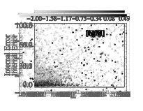
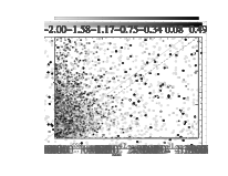
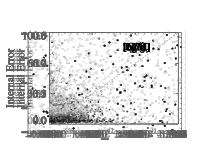
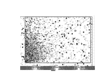
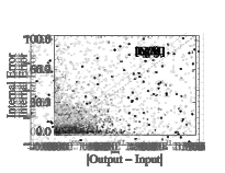
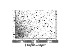
Figure 7.— ferre internal parameter errors versus error estimates from differences between input and output parameters of synthetic spectra. Results are presented for the off-node ($S/N$=100) test with the curvature matrix (left panels) and the multiple search error (right panels) options. Shading indicates metallicity and dashed lines show the one-to-one relation.

6.4. Test D. Effect of Masking Windows in the Global Fit

$H$-band spectra from the ground suffer substantial degradation from Earth’s atmosphere, which imprints OH emission lines and absorption by O₂, CH₄, H₂O, and CO₂. Depending on the strength of these features, their presence and removal increase the uncertainties in the observed fluxes, in some cases to the point that data become useless at particular wavelengths. The fluxes at wavelengths significantly affected by these features of CH₄, H₂O, and CO₂ are weighted according to the uncertainties in the telluric-corrected fluxes.

We have evaluated their impact (Test D in Table 4) by using the actual error bars associated with the APOGEE spectrum of the star 2M18161497-1738507 (APOGEE field 4339, $l=14\arcdeg$, $b=0\arcdeg$) to identify the spectral windows to mask in our synthetic spectra. The star was selected arbitrarily among those with only one APOGEE visit to avoid uncertainties associated with the combination of multiple visits. Some 17% of the total number of pixels are rendered unusable in this particular spectrum, which is a typical figure for the APOGEE data. The analysis results for the $S/N=100$ realization for the off-nodes sample with blocked spectral windows do not show a significant degradation compared to the analysis of the same data set without blocked windows, nor do they show significantly larger errors.

6.5. Test E. Uncertainties Associated with Modeling the Line Spread Function

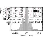
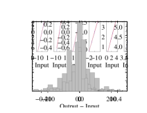
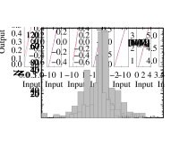
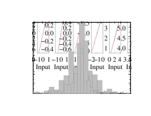
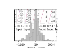
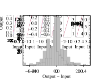
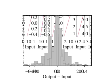
Figure 8.— The distribution of the parameter (output$\ -\$input) differences for the LSF test that uses a $R=18,500$ (left) and a DR12 LSF (right) library to analyze synthetic spectra of $R=22,500$. Each row is for a different parameter.

The APOGEE LSF is not a Gaussian and changes significantly along the pseudoslit (i.e., with fiber) and wavelength (Nidever et al. 2015, Wilson et al., in preparation). Inaccurate LSF modeling in the spectral analysis can introduce uncertainties in ASPCAP parameter determinations, especially for $T_{\rm{eff}}$, $\log{g}$, and $\xi_{\rm{t}}$. ASPCAP went from employing a Gaussian LSF kernel of constant resolving power $R=22,500$ in DR10 to a more realistic LSF shape in DR12. The DR12 LSF was varied as a function of wavelength, based on the average LSF for five different fibers spread across the slit, but the same LSF was adopted for all spectra.

We have evaluated the effect of the LSF approximation we have been using by carrying out two experiments: (1) analyzing spectra from a library convolved with a Gaussian LSF equivalent to $R=22,500$ with a library for $R=18,000$, and (2) analyzing the same spectra using the DR12 equivalent 7D library. In both tests we used the reduced on-node sample and noiseless spectra. The choice of the low resolution Gaussian was to investigate the effect of assuming a wrong spectral resolution in the analysis (a possible case for some fibers in DR10/DR12). We used a rather drastically mismatched resolution to test an extreme case. The test with the DR12 library helped to study the effect of adopting a wrong LSF shape+resolution for the ASPCAP parameter determinations. In this second test we used a Gauss-Hermite LSF of variable $R$ to analyze Gaussian convolved spectra of constant $R$. A similar magnitude of effect would be expected for the inverse case, which roughly accords with the APOGEE DR10 analysis.

Figure 8 and the final three lines of Table 4 (Test E) summarize the results of the test with the correct LSF (for a comparison reference), and of the other two tests. The analysis of the spectra adopting an erroneously low spectral resolution shows that the impact of this systematic can be significant for some parameters. Overall the impacts of assuming an incorrect spectral resolution or assuming an incorrect LSF shape and wavelength dependence, on top of the PCA compression and the cubic interpolation, are comparable in magnitude. Reassuringly, the median offsets are small in both tests: below 0.025 dex in [M/H] and about $-16$ K in $T_{\rm{eff}}$ and $-0.09$ dex in $\log{g}$. The largest median offset is for [N/M], which rises by 0.03–0.04 dex. However, the distribution of offsets is fairly broad for $T_{\rm{eff}}$, [C/M], and [N/M], and $\log{g}$, with dispersions of $\approx 40$ K, 0.07 dex, 0.24 dex, and 0.09 dex, respectively, and some extreme outliers, not significant different from the equivalent test with the right LSF modeling. The values of $T_{\rm{eff}}$, $\log{g}$, and $\xi_{\rm{t}}$ are affected most by the LSF accuracy, severely at high surface gravity for the case of $T_{\rm{eff}}$ and $\log{g}$.

The errors in DR10 parameters associated with inaccurate LSF modeling should be comparable to those shown in our second test. The corresponding errors in DR12 should be smaller, because these ASPCAP analyses incorporate the non-Gaussian and wavelength-dependent LSF, and their main omission is the fiber-to-fiber variation. Comparing to the results of Test C, the effects of LSF modeling errors are larger (typically by a factor of 1.5–2.0) than those of interpolation errors and noise at the level of $S/N=100$. (Note that the reduced on-nodes sample used in Test E is five times smaller than the off-nodes sample used in Test C, 194 versus  1000 spectra.) While median offsets remain small compared to our accuracy goals, the dispersions suggest that imperfect LSF modeling may still contribute non-negligibly to the ASPCAP error budget, particularly for the surface gravity, and for some classes of stars.

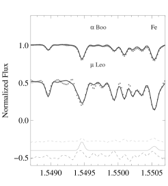
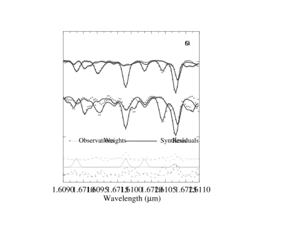
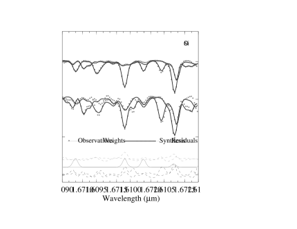
Figure 9.— FTS spectrum (circles) and best spectral synthesis (black solid line) for Arcturus ($\alpha$ Boo) and $\mu$ Leo, for small spectral windows targeted to different chemical elements. Wavelengths are vacuum values. Fits for iron (left), silicon (middle), and silicon (right) are presented, along with the abundance weights (grey solid line) described in Section 4.3. Residuals between the 1-m- and the FTS-spectrum are also presented (dashed lines, top: Arcturus, bottom: $\mu$ Leo). Spectra, residuals and weights are shifted to fit the figure and the weights are also scaled for visibility.

7. Examples with real data

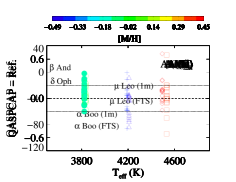
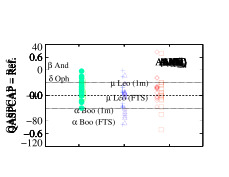
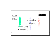
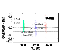
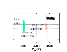
Figure 10.— Stellar parameters and abundances differences (qascap$\ -\$reference) for four well studied stars. For Arcturus and $\mu$-Leo we show both FTS and 1-m+APOGEE results, yielding six points in each test. Data are colored according to their stellar metallicity derived from the global fit ([M/H]). The reference values for the comparison are from Smith et al. (2013). Differences for metallicities derived from both the global fit and dedicated Fe spectral windows are presented and seen to be nearly identical. The dashed and the dotted lines denote 0 and $\pm 0.2$ dex differences, respectively.

The pipeline was tested on real data using high quality ($S/N>100$, $R\geq 45,000$) $H$-band spectra for a set of bright field giants with previously derived abundances in the literature. The test data were obtained with the Fourier Transform Spectrograph (FTS) at the 4-m Mayall Telescope on Kitt Peak. The stars are the giants Arcturus ($\alpha$ Boo), $\beta$ And, $\delta$ Oph, and $\mu$ Leo. The stellar parameter coverage is $3825\leq$ $T_{\rm{eff}}$ $\leq 4550$ K, $0.90\leq\$$\log{g}$$\ \leq 1.70$ and $-0.47\leq$ [Fe/H] $\leq+0.31$. The spectra were smoothed with a Gaussian kernel to the APOGEE nominal spectral resolution of $R=22,500$. Observations of Arcturus and $\mu$ Leo taken with the APOGEE spectrograph linked to the New Mexico State University 1-m telescope at APO (Feuillet et al., in preparation) are also available and were used in our tests. All spectra were analyzed with seven free parameters, using a quick version of ASPCAP (qaspcap). Gaussian and DR12 LSF libraries were adopted in the analysis of the non-APOGEE and 1m-spectra, respectively. Table 5 gives the stellar parameters and chemical abundances from the analysis, along with reference values from Smith et al. (2013). Figure 9 illustrates the quality of the spectral fits for the O, Si and Fe lines of Arcturus and $\mu$ Leo, along with the differences between the spectra from different sources.

7.1. Arcturus

The Sun is a solid reference for spectroscopic studies of main-sequence stars, but Arcturus can be considered as a more appropriate one for studies of giant stars, which are the bulk of APOGEE targets. The APOGEE line list is based on a solar and Arcturus analysis (Shetrone et al. 2015). In this study, we analyzed two Arcturus spectra, the FTS atlas (Hinkle et al., 1995, $R=100,000$) degraded to the APOGEE spectral resolution, and the APOGEE 1m-spectrum.

Figure 10 shows a comparison of the stellar parameters and chemical abundances derived with qaspcap with those in Smith et al. (2013). The latter study reported abundances from the manual analysis of the FTS spectra with a different line list and method than ASPCAP. Note that Smith el al. (2013) derived $T_{\rm{eff}}$ from photometric calibrations and $\log{g}$ from luminosity along with stellar evolution models, while ASPCAP derives them purely spectroscopically. Differences in the derived stellar parameters for the studied stars (e.g., $T_{\rm{eff}}$ and $\log{g}$ values), as well as differences in the atomic data in the adopted line lists, can introduce abundance offsets with respect to their results. Also, the use of slightly different features for abundance determinations in this study and Smith et al. (2013; see Section 4.3) could be responsible for part of the differences in the abundances.

The use of the Arcturus atlas spectrum removes the parameter/abundance uncertainties associated with the modeling of the LSF. Our analysis of those data delivers effective temperature, metallicity, and microturbulent velocity values which are overall in good agreement with the results by Smith et al. (see blue crosses in Figure 10). Compared to Smith et al., ASPCAP finds Arcturus to be slightly cooler and more metal-rich, with offsets of $-85$ K and $+0.04$ dex, and to have slightly higher $\xi_{\rm{t}}$ ($+0.06$ km s^-1)—see Table 5. The agreement for $\log{g}$ is worse; ASCPAP infers a higher $\log{g}$ by $\sim+0.4$ dex, well outside the estimated 0.1 dex uncertainty reported by Smith et al. This discrepancy highlights the need to calibrate ASPCAP-derived values of $\log{g}$ against empirical data. Both DR10 and DR12 release calibrated $\log{g}$ values in addition to the direct ASPCAP estimates (see Mészáros et al. 2013 and Holtzman et al. 2015 for more details).

We find good agreement with Smith et al. (2013) for the elemental abundances, with differences that are typically smaller than or of the order of their estimated uncertainties. The elements for which we find the best agreement ($<0.05$ dex) are Fe, Ca, and Mn. They are followed by the abundance of Ni, with an offset less than $0.1$ dex. Offsets of about 0.2 dex or larger are observed for N, O, Si, K, and V. In the case of Si, the discrepancy between the results is larger than the estimated uncertainty, and it is probably related to our adoption of smaller $\log{gf}$ values for the Si i lines. Different ${\log{gf}}$s can also be responsible for the large abundance offset for K. For other elements, however, the differences in $\log{gf}$ in the adopted line lists were typically smaller than 0.1 dex.

The APOGEE 1m-spectrum has high $S/N$ but suffers from distortions associated with the persistence in the detectors (see Majewski et al. 2015, Nidever et al. 2015), a complex LSF, and other factors that can degrade the performance of ASPCAP. Nonetheless, the results of our analysis are overall in good agreement with the reference values of Smith et al. (2013), and comparable to that obtained from the analysis of the Arcturus atlas spectrum (compare triangles versus crosses in Figure 10). The exception is the microturbulent velocity, which has an offset of $-0.43$ km s^-1 for the 1-m spectrum, significantly larger than that obtained for the Atlas spectrum ($+0.06$ km s^-1). The DR12 analysis however fixes $\xi_{\rm{t}}$ based on $\log{g}$ (see §3.5), yielding a value $\xi_{\rm t}=1.82\,$km s^-1 that is only 0.04 km s^-1 below Smith et al’s value. Other DR12 stellar parameters for Arcturus agree well with those found here for an analysis with the $\xi_{\rm{t}}$ as a free parameter: $T_{\rm{eff}}$$\ =4206$ K, $\log{g}$$\ =2.01$ [cgs], and [M/H]$\ =-0.54$. The exception to this agreement is for the 1-m spectrum microturbulent velocity. Elemental abundance differences between the Atlas and 1-m analyses are generally small, indicating little sensitivity to details of the data and LSF. The abundances showing the largest differences ($0.15-0.2$ dex) are N, Al, Ti, and V. We note that the abundances of especially Ti, Si, and Al, along with $\log{g}$ and $\xi_{\rm{t}}$, are sensitive to the adopted LSF modeling (Gaussian versus a DR12 LSF) in the analysis of the 1m-spectrum.

7.2. Analysis of Other Stars

We analyzed the FTS spectra of the super-solar metallicity red giant $\mu$ Leo ([Fe/H] $=+0.31$) and the cool red giants $\beta$ And, and $\delta$ Oph ($T_{\rm{eff}}$ $\lesssim 3900$ K), and the 1m-spectrum of $\mu$ Leo. The FTS spectra were retrieved from the Kitt Peak National Observatory archive (Hall et al., 1979). This sample allows us to test ASPCAP results in a more metal-rich regime than the one probed in the analysis of Arcturus discussed above.

The differences between the results obtained for $\mu$ Leo (red diamond), $\beta$ And (filled green circle), and $\delta$ Oph (empty green circle) using ASPCAP and those from the manual analysis in Smith et al. (2013) are also shown as a function of $T_{\rm{eff}}$ in Figure 10. At these higher metallicities the agreement between the stellar parameters from ASPCAP and Smith et al. (2013) remains good (see top panel of Figure 10), similar or in some cases even better than for Arcturus. In general, and in particular for surface gravity and microturbulence, there seems to be an indication of a dependence on the effective temperature of the star.

• Surface gravity: overall there seems to be a systematic difference between the surface gravities derived by ASPCAP and Smith et al. (2013) in the sense that ASPCAP results are systematically larger. The differences found for the surface gravities of $\beta$ And, and $\delta$ Oph are $\sim 0.2-0.3$ dex, but for the most most metal rich and hottest star in our sample, $\mu$ Leo, the discrepancy is significant ($+0.68$ dex) and much larger than the expected uncertainties in Smith et al. (2013).

• Microturbulence: as noted previously, there seems to be an overall trend with effective temperature. However, the microturbulent velocities generally agree with Smith et al. to within 0.4 km s^-1 for the three stars.

• Metallicities: the global metallicities agree with those of Smith et al. (2013), to within 0.04, 0.01, and 0.14 dex ($\beta$ And, $\delta$ Oph, and $\mu$ Leo, respectively). Agreement of Fe abundances is still better.

Our individual chemical abundances match those presented in Smith et al. (2013), with differences typically smaller than $0.2$ dex. The best agreement is found for Ca. For some of the elements, there is a suggestive trend of the abundance differences with the effective temperature of the stars, e.g., for C and Ni, and perhaps a marginal trend for Fe, Mg, and Ca. Of course, with only four stars, two of similar temperature, the ability to reliably identify such trends is limited. For $\mu$ Leo, the $\log{g}$ offset of +0.68 dex significantly affects the derived C abundance and may be responsible for the worse agreement on [C/M]. There is also some dependence of the abundance differences with Smith et al. on [M/H] for some of the elements, e.g., N, O and V. The trends of the abundance differences with $T_{\rm{eff}}$ and [M/H] may result from the different stellar parameters adopted by Smith et al.

Some of the elements with the most discrepant abundances for Arcturus (N, O, K, and Si), are also discrepant for some of the other test stars, differing by $\gtrsim 0.15$ dex from the values of Smith et al. (2013). However, these differences are still within the uncertainties estimated by Smith et al. Only Si systematically exceeds the Smith et al. value in all the stars by an amount larger than expected errors, further supporting the idea that atomic data are a major contributor to the differences between these two studies. There is dispersion in the K abundance offset with Smith et al. (2013), which rules out the atomic data as the major source of discrepancy. Other elements that show larger-than-expected discrepancies are Mg ($\beta$ And) and Mn ($\delta$ Oph).

The result obtained from the APOGEE 1m-spectrum of $\mu$ Leo (red squares in Figure 10) are similar to those from the FTS spectrum. The parameters that depend the most on which observations are adopted are, as in the case of Arcturus, the effective temperature and microturbulence.

In summary, there is good overall agreement between our abundances and those of Smith et al. (2013). The dispersion (standard deviation) of abundance differences is $<0.10$ dex. The abundances of Ca, Fe, and Ni (with the exception of $\mu$ Leo) generally agree quite well, while our most discrepant abundances are Si (not surprising given the differences in adopted atomic data). Abundance differences with the values in Smith et al. (2013) are due partly to the differences in the stellar parameters, in the atomic data, and/or in the analyzed spectra. The microturbulent velocity, in particular, changes significantly depending on the source of the spectra.

Table 5Stellar Parameter and Chemical Abundances

	$\alpha$ Boo			$\beta$ And		$\delta$ Oph		$\mu$ Leo
	FTS	1-m	Ref.	FTS	Ref.	FTS	Ref.	FTS	1-m	Ref.
$T_{\rm{eff}}$ (K)	$+4189$	$+4207$	$+4275$	$+3823$	$+3825$	$+3832$	$+3850$	$+4492$	$+4530$	$+4550$
$\log{g}$ (cgs)	$+2.09$	$+2.02$	$+1.70$	$+1.17$	$+0.90$	$+1.39$	$+1.20$	$+2.78$	$+2.76$	$+2.10$
$\xi_{\rm{t}}$ (km s-1)	$+1.92$	$+1.43$	$+1.86$	$+2.32$	$+2.19$	$+2.25$	$+1.91$	$+1.95$	$+1.28$	$+1.82$
$[\mathrm{M}/\mathrm{H}]$	$-0.43$	$-0.49$	$-0.47$	$-0.18$	$-0.22$	$+0.00$	$-0.01$	$+0.45$	$+0.35$	$+0.31$
A(Fe)	$+7.00$	$+6.95$	$+6.98$	$+7.23$	$+7.23$	$+7.41$	$+7.44$	$+7.88$	$+7.76$	$+7.76$
A(C)	$+8.09$	$+7.99$	$+7.96$	$+8.05$	$+8.06$	$+8.27$	$+8.24$	$+8.80$	$+8.69$	$+8.52$
A(N)	$+7.45$	$+7.29$	$+7.64$	$+7.96$	$+8.05$	$+8.03$	$+8.20$	$+8.69$	$+8.53$	$+8.71$
A(O)	$+8.45$	$+8.39$	$+8.64$	$+8.58$	$+8.78$	$+8.71$	$+8.77$	$+9.16$	$+9.04$	$+9.05$
A(Mg)	$+7.27$	$+7.19$	$+7.15$	$+7.48$	$+7.26$	$+7.58$	$+7.54$	$+7.89$	$+7.79$	$+7.85$
A(Al)	$+5.99$	$+6.21$	$+6.16$	$+6.26$	$+6.12$	$+6.53$	$+6.45$	$+6.87$	$+6.87$	$+6.90$
A(Si)	$+7.41$	$+7.31$	$+7.12$	$+7.48$	$+7.18$	$+7.71$	$+7.53$	$+8.03$	$+7.96$	$+7.76$
A(K)	$+4.63$	$+4.58$	$+4.79$	$+4.75$	$+4.86$	$+5.32$	$+5.18$	$+5.58$	$+5.33$	$+5.63$
A(Ca)	$+5.88$	$+5.83$	$+5.84$	$+6.08$	$+6.02$	$+6.21$	$+6.24$	$+6.54$	$+6.55$	$+6.62$
A(Ti)	$+4.46$	$+4.62$	$+4.59$	$+4.90$	$+4.72$	$+5.02$	$+5.07$	$+5.52$	$+5.44$	$+5.40$
A(V)	$+3.43$	$+3.29$	$+3.61$	$+3.76$	$+3.66$	$+3.92$	$+3.86$	$+4.28$	$+4.34$	$+4.18$
A(Mn)	$+4.90$	$+4.88$	$+4.86$	$+5.27$	$+5.18$	$+5.57$	$+5.34$	$+5.89$	$+5.89$	$+5.79$
A(Ni)	$+5.84$	$+5.83$	$+5.77$	$+6.02$	$+6.01$	$+6.21$	$+6.18$	$+6.73$	$+6.60$	$+6.60$

7.3. The Open Cluster M67

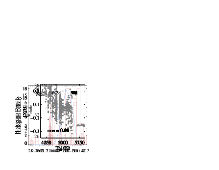
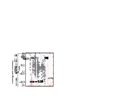
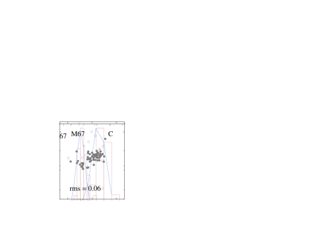
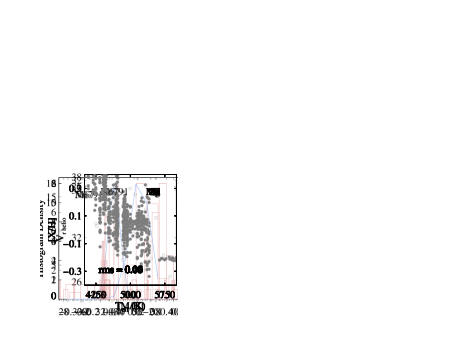
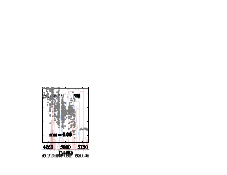
Figure 11.— The DR12 heliocentric radial velocities and chemical abundances for a sample of $\sim 30$ M67 members. The filled circles in top-left panel denote velocity and [M/H] (from the global fit) cluster membership, and the empty circles represent outliers. The other panels show examples of elements with high (O, Ca, and Fe), and low (Si, Ti, and Mn) precision estimates. Abundances are shown versus $T_{\rm{eff}}$.

Stellar clusters are ideal benchmarks to calibrate abundance determinations. Stars in clusters share essentially the same chemical content, though some globular clusters and/or chemical elements show some variations associated with multiple populations or with mixing processes. Abundance trends with $T_{\rm{eff}}$ are an indication of systematic uncertainties, providing that mixing processes are not altering the chemical composition.

APOGEE observed several clusters in a wide metallicity range, including the very well studied solar-metallicity open cluster M67. The APOGEE results for the cluster show ASPCAP abundances of high precision. Our cluster membership is based on a combination of photometry, radial velocity, and metallicity information. We redefined the sample using a $\sim 3.0\times\sigma$ (Gaussian) cut in both radial velocity and metallicity. DR12 heliocentric radial velocities and direct ASPCAP chemical abundances (without the calibration offsets applied to DR12 as described by Holtzman et al. 2015) are presented in Figure 11. Cluster members and outliers are presented in top panel. The cluster radial velocity and [M/H] derived from the Gaussian fits to the parameters distribution of the cluster members are 33.51 km s^-1 (standard deviation of 0.66 km s^-1) and 0.03 (standard deviation of 0.04 dex), respectively. A similar metallicity value of 0.06 is obtained from iron lines.

The lower panels of Figure 11 plot DR12 values of [X/H] versus $T_{\rm{eff}}$, after eliminating non-cluster members, and stars flagged as BAD or with BAD abundances (treating each chemical element separately). The O, Ca, and Fe abundances show small dispersion (0.03-0.04 dex) and little or no trend with $T_{\rm{eff}}$. The Si, Ti, and Mn abundances show clear trends with $T_{\rm{eff}}$ that likely indicate systematic ASPCAP errors in this $4250-5500\,{\rm K}$ temperature range. The dispersion around this trend remains small, and even with the trend the dispersion of values is only 0.08-0.09 dex. Larger dispersions are found for N and V (not shown in the figure), though the former may be affected by mixing processes. Holtzman et al. (2015) present comparisons to a wider range of open cluster data and derive temperature-dependent abundance calibration offsets element by element, which are applied to the APOGEE DR12 release.

8. Conclusions

ASPCAP is the pipeline for deriving stellar parameters and chemical abundances from APOGEE spectra. The pipeline matches the observations to a set of synthetic spectrum templates using the $\chi^{2}$ minimization in a multidimensional parameter space. Stellar parameters are derived first from the entire APOGEE spectral range, followed by the determination of individual chemical abundances from spectral windows optimized for each element. The precision and the level of sophistication of the high-dimensional analysis that ASPCAP performs is unprecedented in such a large volume of data.

ASPCAP has three main components: the model spectral libraries, the ferre optimization code that searches for the best fit, and the IDL wrapper for book-keeping and data pre- and post-processing. In this paper we described each component and presented the pipeline configuration used in DR10 (Ahn et al., 2014) and DR12 (Alam et al., 2015). The employed algorithms have proven to work well with both simulations and observations.

Random abundance uncertainties are expected to be typically $<0.1$ dex, based on tests with simulations, and the DR12 results for M67. For accuracy, we expect typically $\lesssim 0.20$ dex based on the comparison of our abundance results with the values of Smith et al. (2013) for a set of reference stars.

Some of the issues we have detected include:

• Our tests indicate that a detailed modeling of the LSF is important and the systematic effects associated with poor LSF matching may be appreciable. An empirical LSF has been used for DR12 versus a Gaussian LSF of constant $R$ for DR10.

• PCA compression of the synthetic libraries may affect ASPCAP results for low metallicity spectra ([M/H]$\ <-1$), which lie outside the bulk of the APOGEE sample, but, nonetheless, requires further investigation.

• Due to the lack of information in metal-poor or warm spectra, ASPCAP’s performance is poorer for these cases, and an alternative strategy, where fewer parameters are involved in the modeling, is needed in these regions of the parameter space.

• There are significant uncertainties in the inferred nitrogen abundances, as a result of the modest sensitivity of CN lines to changes in the N abundance.

ASPCAP continues to evolve and efforts concentrate now on addressing issues such as extending the parameter coverage, establishing abundance upper limits to the abundances from undetected spectral lines, and improving the LSF modeling. Spectral libraries for cooler stars are already available and will be incorporated soon.

We plan to investigate whether individual elemental abundances can be fit independently of each other to deliver more accurate abundances. The larger APOGEE-2 project of SDSS-IV brings additional motivation for continuing the development of ASPCAP.

We acknowledge funding from NSF grants AST11-09718 and AST-907873. Funding for SDSS-III has been provided by the Alfred P. Sloan Foundation, the Participating Institutions, the National Science Foundation, and the U.S. Department of Energy Office of Science. The SDSS-III website is http://www.sdss3.org/. SDSS-III is managed by the Astrophysical Research Consortium for the Participating Institutions of the SDSS-III Collaboration including the University of Arizona, the Brazilian Participation Group, Brookhaven National Laboratory, University of Cambridge, Carnegie Mellon University, University of Florida, the French Participation Group, the German Participation Group, Harvard University, the Instituto de Astrofisica de Canarias, the Michigan State/Notre Dame/JINA Participation Group, Johns Hopkins University, Lawrence Berkeley National Laboratory, Max Planck Institute for Astrophysics, Max Planck Institute for Extraterrestrial Physics, New Mexico State University, New York University, Ohio State University, Pennsylvania State University, University of Portsmouth, Princeton University, the Spanish Participation Group, University of Tokyo, University of Utah, Vanderbilt University, University of Virginia, University of Washington, and Yale University.

Support for A.E.G.P. was provided by SDSS-III/APOGEE. C.A.P. is thankful for support from the Spanish Ministry of Economy and Competitiveness (MINECO) through grant AYA2014-56359-P. Sz.M. has been supported by the János Bolyai Research Scholarship of the Hungarian Academy of Sciences. D.A.G.H., and O.Z. acknowledge support provided by the Spanish Ministry of Economy and Competitiveness under grant AYA-2011-27754 and AYA2014-58082-P.

References

- Ahn et al. (2014) Ahn, C. P., Alexandroff, R., Allende Prieto, C., et al. 2014, ApJS, 211, 17
- Alam et al. (2015) Alam, S., Albareti, F. D., Allende Prieto, C., et al. 2015, ApJS, 219, 12
- Allende Prieto et al. (2006) Allende Prieto, C., Beers, T. C., Wilhelm, R., et al. 2006, ApJ, 636, 804
- Allende Prieto et al. (2014) Allende Prieto, C., Fernández-Alvar, E., Schlesinger, K. J., et al. 2014, A&A, 568, A7
- Asplund et al. (2005) Asplund, M., Grevesse, N., & Sauval, A. J. 2005, Cosmic Abundances as Records of Stellar Evolution and Nucleosynthesis, 336, 25
- Asplund et al. (2009) Asplund, M., Grevesse, N., Sauval, A. J., & Scott, P. 2009, ARA&A, 47, 481
- Beers et al. (1985) Beers, T. C., Preston, G. W., & Shectman, S. A. 1985, AJ, 90, 2089
- Castelli & Kurucz (2004) , Castelli, F., & Kurucz, R. L. 2004, [arXiv:astro-ph/0405087]
- Castelli (2005) Castelli, F. 2005, Memorie della Societa Astronomica Italiana Supplementi, 8, 25
- Christlieb (2003) Christlieb, N. 2003, Reviews in Modern Astronomy, 16, 191
- Eisenstein et al. (2011) Eisenstein, D. J., Weinberg, D. H., Agol, E., et al. 2011, AJ, 142, 72
- Freeman et al. (2013) Freeman, K., Ness, M., Wylie-de-Boer, E., et al. 2013, MNRAS, 428, 3660
- García Pérez et al. (2006) García Pérez, A. E., Asplund, M., Primas, F., Nissen, P. E., & Gustafsson, B. 2006, A&A, 451, 621
- García Pérez et al. (2013) García Pérez, A. E., Cunha, K., Shetrone, M., et al. 2013, ApJ, 767, L9
- Gilmore et al. (2012) Gilmore, G., Randich, S., Asplund, M., et al. 2012, The Messenger, 147, 25
- González Hernández & Bonifacio (2009) González Hernández, J. I., & Bonifacio, P. 2009, A&A, 497, 497
- Grevesse & Sauval (1998) Grevesse, N., & Sauval, A. J. 1998, Space Sci. Rev., 85, 161
- Gunn et al. (2006) Gunn, J. E., Siegmund, W. A., Mannery, E. J., et al. 2006, AJ, 131, 2332
- Gustafsson et al. (2008) Gustafsson, B., Edvardsson, B., Eriksson, K., et al. 2008, A&A, 486, 951
- Hall et al. (1979) Hall, D. N. B., Ridgway, S., Bell, E. A., & Yarborough, J. M. 1979, Proc. SPIE, 172, 121
- Hinkle et al. (1995) Hinkle, K., Wallace, L., & Livingston, W. 1995, PASP, 107, 1042
- Holtzman et al. (2015) Holtzman, J. A., Shetrone, M., Johnson, J. A., et al. 2015, arXiv:1501.04110
- Koesterke et al. (2008) Koesterke, L., Allende Prieto, C., & Lambert, D. L. 2008, ApJ, 680, 764
- Koesterke (2009) Koesterke, L. 2009, American Institute of Physics Conference Series, 1171, 73
- Lee et al. (2008) Lee, Y. S., Beers, T. C., Sivarani, T., et al. 2008, AJ, 136, 2022
- Majewski (2012) Majewski, S. R. 2012, American Astronomical Society Meeting Abstracts #219, 219, #205.06
- Mészáros & Allende Prieto (2013) Mészáros, S., & Allende Prieto, C. 2013, MNRAS, 430, 3285
- Mészáros et al. (2012) Mészáros, S., Allende Prieto, C., Edvardsson, B., et al. 2012, AJ, 144, 120
- Mészáros et al. (2013) Mészáros, S., Holtzman, J., García Pérez, A. E., et al. 2013, AJ, 146, 133
- Nelder & Mead (1965) Nelder, J. A. & Mead, R. 1965,The Computer Journal, 7, 308
- Nidever et al. (2015) Nidever, D. L., Holtzman, J. A., Allende Prieto, C., et al. 2015, arXiv:1501.03742
- Randich et al. (2013) Randich, S., Gilmore, G., & Gaia-ESO Consortium 2013, The Messenger, 154, 47
- Skrutskie et al. (2006) Skrutskie, M. F., Cutri, R. M., Stiening, R., et al. 2006, AJ, 131, 1163
- Pearson (1991) Pearson, K. 1901, Philosophical Magazine, 2, 559
- Press et al. (2007) Press, W. H.; Teukolsky, S. A.; Vetterling, W. T.; Flannery, B. P. 2007, Numerical Recipes: The Art of Scientific Computing (3rd ed.). New York: Cambridge University Press
- Pence et al. (2010) Pence, W. D., Chiappetti, L., Page, C. G., Shaw, R. A., & Stobie, E. 2010, A&A, 524, AA42
- Rousselot et al. (2000) Rousselot, P., Lidman, C., Cuby, J.-G., Moreels, G., & Monnet, G. 2000, A&A, 354, 1134
- Smiljanic et al. (2014) Smiljanic, R., Korn, A. J., Bergemann, M., et al. 2014, A&A, 570, AA122
- Smith et al. (2013) Smith, V. V., Cunha, K., Shetrone, M. D., et al. 2013, ApJ, 765, 16
- Lee et al. (2008) Lee, Y. S., Beers, T. C., Sivarani, T., et al. 2008, AJ, 136, 2022
- Skrutskie et al. (2006) Skrutskie, M. F., Cutri, R. M., Stiening, R., et al. 2006, AJ, 131, 1163
- Steinmetz et al. (2006) Steinmetz, M., Zwitter, T., Siebert, A., et al. 2006, AJ, 132, 1645
- Wilson et al. (2012) Wilson, J. C., Hearty, F., Skrutskie, M. F., et al. 2012, Proc. SPIE, 8446,
- Xiang et al. (2015) Xiang, M. S., Liu, X. W., Yuan, H. B., et al. 2015, MNRAS, 448, 822
- Yanny et al. (2009) Yanny, B., Rockosi, C., Newberg, H. J., et al. 2009, AJ, 137, 4377
- Zamora et al. (2015) Zamora, O., García-Hernández, D. A., Allende Prieto, C., et al. 2015, AJ, 149, 181
- Zasowski et al. (2013) Zasowski, G., Johnson, J. A., Frinchaboy, P. M., et al. 2013, AJ, 146, 81
- Zhao et al. (2012) Zhao, G., Zhao, Y.-H., Chu, Y.-Q., Jing, Y.-P., & Deng, L.-C. 2012, Research in Astronomy and Astrophysics, 12, 723