Variability in a Young, L/T Transition Planetary Mass Object

Abstract

As part of our ongoing NTT SoFI survey for variability in young free-floating planets and low mass brown dwarfs, we detect significant variability in the young, free-floating planetary mass object PSO J318.5-22, likely due to rotational modulation of inhomogeneous cloud cover. A member of the 23$\pm$3 Myr $\beta$ Pic moving group, PSO J318.5-22 has T_eff = 1160${}^{+30}_{-40}$ K and a mass estimate of 8.3$\pm$0.5 M_Jup for a 23$\pm$3 Myr age. PSO J318.5-22 is intermediate in mass between 51 Eri b and $\beta$ Pic b, the two known exoplanet companions in the $\beta$ Pic moving group. With variability amplitudes from 7-10$\%$ in J_S at two separate epochs over 3-5 hour observations, we constrain the rotational period of this object to $>$5 hours. In K_S, we marginally detect a variability trend of up to 3$\%$ over a 3 hour observation. This is the first detection of weather on an extrasolar planetary mass object. Among L dwarfs surveyed at high-photometric precision ($<$3$\%$) this is the highest amplitude variability detection. Given the low surface gravity of this object, the high amplitude preliminarily suggests that such objects may be more variable than their high mass counterparts, although observations of a larger sample is necessary to confirm this. Measuring similar variability for directly imaged planetary companions is possible with instruments such as SPHERE and GPI and will provide important constraints on formation. Measuring variability at multiple wavelengths can help constrain cloud structure.

1. Introduction

Of the current ensemble of $\sim$30 free-floating young planetary mass objects (Gagné et al., 2014, 2015), PSO J318.5-22 (Liu et al., 2013) is the closest analogue in properties to imaged exoplanet companions. Gagné et al. (2014) and Liu et al. (2013) identify it as a $\beta$ Pic moving group member (23$\pm$3 Myr, Mamajek & Bell, 2014) and it possesses colors and magnitudes similar to the HR 8799 planets (Marois et al., 2008, 2010) and 2M1207-39b (Chauvin et al., 2005). PSO J318.5-22 has T_eff = 1160${}^{+30}_{-40}$ K and a published mass estimate of 6.5${}^{+1.3}_{-1.0}$ M_Jup for an age of 12 Myr (Liu et al., 2013), rising to 8.3$\pm$0.5 M_Jup for the updated age of 23$\pm$3 Myr (Allers et al. submitted). PSO J318.5-22 is intermediate in mass and luminosity between 51 Eri b ($\sim$2 M_Jup, Macintosh et al., 2015) and $\beta$ Pic b ($\sim$11-12 M_Jup, Lagrange et al., 2010; Bonnefoy et al., 2014), the two known exoplanet companions in the $\beta$ Pic moving group. Because PSO J318.5-22 is free-floating, it enables high precision characterization not currently possible for exoplanet companions to bright stars. In particular, we report here the first detection of photometric variability in a young, L/T transition planetary mass object.

Variability is common for cool brown dwarfs but until now has not been probed for lower-mass planetary objects with similar effective temperatures. Recent large-scale surveys of brown dwarf variability with Spitzer have revealed mid-IR variability of up to a few percent in $>$50% of L and T type brown dwarfs (Metchev et al., 2015). Buenzli et al. (2014) find that $\sim$30% of the L5-T6 objects surveyed in their HST SNAP survey show variability trends and large ground-based surveys also find widespread variability (Radigan et al., 2014; Wilson et al., 2014; Radigan, 2014). While variability amplitude may be increased across the L/T transition (Radigan et al., 2014), variability is now robustly observed across a wide range of L and T spectral types. We therefore expect variability in young extrasolar planets, which share similar T_eff and spectral types but lower surface gravity. In fact, Metchev et al. (2015) tentatively find a correlation between low surface gravity and high-amplitude variability in their L dwarf sample.

Observed field brown dwarf variability is likely produced by rotational modulation of inhomogenous cloud cover over the 3-12 hour rotational periods of these objects (Zapatero Osorio et al., 2006). Apai et al. (2013) and Buenzli et al. (2015) find that their variability amplitude as a function of wavelength are best fit by a combination of thin and thick cloud layers. We expect a similar mechanism to drive variability in planetary mass objects with similar T_eff, albeit with potentially longer periods, as these objects will not yet have spun up with age. Only a handful of directly imaged exoplanet companions are amenable to variability searches using high-contrast imagers such as SPHERE at the VLT (Beuzit et al., 2008) and GPI at Gemini (Macintosh et al., 2014); to search for variability in a larger sample of planetary mass objects and young, very low mass brown dwarfs, we have been conducting the first survey for free-floating planet variability using NTT SoFI (Moorwood et al., 1998). We have observed 22 objects to date, of which 7 have mass estimates $<$13 M_Jup and all have mass estimates $<$25 M_Jup. PSO J318.5-22 is the first variability detection from this survey.

2. Observations and Data Reduction

Table 1SOFI observations of PSO J318.5-22

Date	Filter	DIT	NDIT	Exp. Time	On-Sky Time
2014 Oct 9	JS	10 s	6	3.80 hours	5.15 hours
2014 Nov 9	JS	15 s	6	2.40 hours	2.83 hours
2014 Nov 10	KS	20 s	6	2.80 hours	3.16 hours

We obtained 3 datasets for PSO J318.5-22 with NTT SoFI (0.288$\arcsec$/ pixel, 4.92’$\times$4.92’ field of view) in October and November 2014. Observations are presented in Table 1. We attempted to cover as much of the unknown rotation period as possible, however, scheduling constraints and weather conditions limited our observations to 2-5 hours on sky. In search mode, we observed in J_S, however we did obtain a K_S followup lightcurve for PSO J318.5-22. We nodded the target between two positions on the chip, ensuring that, at each jump from position to position, the object is accurately placed on the same original pixel. This allowed for sky-subtraction, while preserving photometric stability. We followed an ABBA nodding pattern, taking three exposures at each nod position.

Data were corrected for crosstalk artifacts between quadrants, flat-fielded using special dome flats which correct for the “shade” (illumination dependent bias) found in SoFI images, and illumination corrected using observations of a standard star. Sky frames for each nod position were created by median combining normalized frames from the other nod positions closest in time. These were then re-scaled to and subtracted from the science frame. Aperture photometry for all sources on the frame were acquired using the IDL task aper.pro with aperture radii of 4, 4.5, 5, 5.5, 6, and 6.5 pixels and background subtraction annuli from 21-31 pixels.

3. Light Curves

We present the final binned J_S lightcurve from October 2014 (with detrended reference stars for comparison) in Fig. 1 and the final binned J_S and K_S lightcurves from November 2014 in Fig. 2. Raw light curves obtained from aperture photometry display fluctuations in brightness due to changing atmospheric transparency, airmass, and residual instrumental effects. These changes can be removed via division of a calibration curve calculated from carefully chosen, well-behaved reference stars (Radigan et al., 2014). To detrend our lightcurves, first we discarded potential reference stars with peak flux values below 10 or greater than 10000 ADU (where array non-linearity is limited to $<$1.5$\%$). Different nods were normalized via division by their median flux before being combined to give a relative flux light curve. For each star a calibration curve was created by median combining all other reference stars (excluding that of the target and star in question). The standard deviation and linear slope for each lightcurve was calculated and stars with a standard deviation or slope $\sim$1.5-3 times greater than that of the target were discarded. This process was iterated until a set of well-behaved reference stars was chosen. Final detrended light curves were obtained by dividing the raw curve for each star by its calibration curve. The best lightcurves shown here are with the aperture that minimizes the standard deviation after removing a smooth polynomial (as done in  Biller et al., 2013) – for all epochs, the 4 pixel aperture (similar to the PSF FWHM) yielded the best result. Final lightcurves are shown binned by a factor of three – combining all three exposures taken in each ABBA nod position. Error bars were calculated in a similar manner as in Biller et al. (2013) – a low-order polynomial was fit to the final lightcurve and then subtracted to remove any astrophysical variability and the standard deviation of the subtracted lightcurve was adopted as the typical error on a given photometric point (shown in each lightcurve as the error bar given on the first photometric point). As a check, we also measured photometry and light curves using both the publically available aperture photometry pipeline from Radigan (2014) as well as the psf-fitting pipeline described in Biller et al. (2013). Results from all three pipelines were consistent.

We found the highest amplitude of variability in our J_S lightcurve from 9 October 2014 – over the five hours observed, PSO J318.5-22 varies by 10$\pm$1.3$\%$. The observed variability does not correlate with airmass changes – the target was overhead for the majority of this observation, with airmass between 1 and 1.2 for the first 3 hours, increasing to $\sim$2 by the end of the observation. The flattening of the lightcurve from 4-5 hours elapsed time in our lightcurve may be indicative of a minimum in the lightcurve. However, as no clear repetition of maxima or minima have been covered, the strongest constraints we can place on the rotational period and variability amplitude for PSO J318.5-22 in this epoch is that the period must be $>$5 hours and the amplitude must be $\geq$10$\%$. If the variation is sinusoidal, these observations point to an even longer period of $>$7-8 hours.

On 9 November 2014, we recovered J_S variability with a somewhat smaller amplitude of 7$\pm$1$\%$ over our three hour long observation. A maximum is seen 1 hour into the observation and a potential minimum is seen at 2 hours into the observation. The observed variability is not correlated with airmass changes during the observation – the observation started at airmass = 1.1, increasing steadily to airmass =2.0 at the end of the observation. If the variability is roughly sinusoidal and single peaked, this observation would suggest a period$\sim$3 hours; however, we cannot constrain the period beyond requiring it to be $>$3 hours, as we have not covered multiple extrema and as the light curve could potentially be double-peaked (Radigan et al., 2012). The lightcurve evolved considerably between the October and November 2014 epochs – a phenomena also found in other older variable brown dwarfs (Radigan et al., 2012, 2014; Artigau et al., 2009; Metchev et al., 2015; Gillon et al., 2013).

On 11 November 2014, we obtained a K_S lightcurve for PSO J318.5-22. Given its extremely red colors, PSO J318.5-22 is brighter in K_S than J_S and is one of the brightest objects in the SoFI field. Thus, we attain higher photometric precision in our K_S (0.7$\%$) lightcurve compared to J_S (1 - 1.3$\%$). Fitting slopes to the target and 3 similarly-bright reference stars, the target increases in flux by 0.9$\%$ per hour while the reference stars have slopes of 0.1-0.6$\%$ / hour (consistent with a flat line within our photometric precision). Thus, we tentatively find a marginal variability trend of up to 3$\%$ over our 3 hour observation, requiring reobservation to be confirmed. Additionally, in this case the tentative variability is not completely uncorrelated with airmass changes – during this observation, airmass increased steadily from 1.1 to 2.2.

Figure 1.— Final binned J_S lightcurve and comparison detrended reference stars from 9 October 2014. Typical error bars are shown on the first photometric point. The variability amplitude at this epoch is $>$10$\%$ with a period of $>$5 hours.

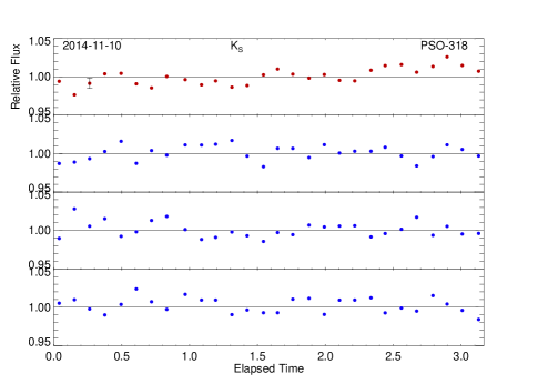
Figure 2.— Top: Final binned J_S lightcurve from 9 November 2014. Bottom: Final binned K_S lightcurve from 11 November 2014. Lightcurves are presented similarly as in Fig. 1. The J_S variability amplitude at this epoch is $>$7$\%$ with a period of $\geq$3 hours. We marginally detect K_S variability, with amplitude up to 3$\%$ over our 3 hour observation.

4. Discussion

This is the first detection of variability in such a cool, low-surface gravity object. While variability has been detected previously for very young ($<$1-2 Myr) planetary mass objects in star-forming regions such as Orion (cf.  Joergens et al., 2013), such variability is driven by a different mechanism than expected for PSO J318.5-22. These previous detections have been for M spectral type objects with much higher T_eff than PSO J318.5-22. At these temperatures, variability is driven by starspots induced by the magnetic fields of these objects or ongoing accretion. PSO J318.5-22 is too cool to have starspots and likely too old for ongoing accretion. From its red colors, PSO J318.5-22 must be entirely cloudy (Liu et al., 2013). Thus the likely mechanism producing the observed variability is inhomogeneous cloud cover, as has been found previously to drive variability in higher mass brown dwarfs with similar T_eff (Artigau et al., 2009; Radigan et al., 2012; Buenzli et al., 2014; Radigan et al., 2014; Radigan, 2014; Wilson et al., 2014; Apai et al., 2013; Buenzli et al., 2015). Notably, among L dwarfs surveyed at high-photometric precision ($<$3$\%$), PSO J318.5-22’s J band variability amplitude is the highest measured for an L dwarf to date (cf. Yang et al. 2015 and Buenzli et al. submitted) – reinforcing the suggestion by Metchev et al. (2015) that variability amplitudes might be typically larger for lower gravity objects.

To model cloud-driven as well as hot-spot variability, we follow the approach of Artigau et al. (2009) and Radigan et al. (2012), combining multiple 1-d models to represent different regions of cloud cover. We consider the observed atmosphere of our object to be composed of flux from two distinct cloud regions (varying in temperature and/or in cloud prescription) with fluxes of $F_{1}$ and $F_{2}$ respectively and with a minimum filling fraction for the $F_{2}$ region of $a$. The peak-to-trough amplitude of variability ($\Delta F$ / $F$, i.e. the change of flux divided by the mid-brightness flux) observed in a given bandpass due a change of filling fraction over the course of the observation is given by Equation 2 from Radigan et al. 2012, where $\Delta$a is the change in filling factor over the observation, $\Delta$F = $F_{2}$ - $F_{1}$, and $\alpha$ = $a$ + 0.5$\Delta a$, the filling fraction of the $F_{2}$ regions at mid-brightness:

$$\begin{array}[]{l}A=\frac{(1-a-\Delta a)F_{1}+(a+\Delta a)F_{2}-(1-a)F_{1}-aF_{2}}{0.5[(1-a-\Delta a)F_{1}+(a+\Delta a)F_{2}+(1-a)F_{1}+aF_{2}]}\\ =\frac{\Delta a}{\alpha+F_{1}/\Delta F}\\ \end{array}$$ (1)

We calculated the synthetic photon fluxes $F_{1}$ and $F_{2}$ using the cloudy exoplanet models of Madhusudhan et al. (2011) and the filter transmissions provided for the SoFI $J_{S}$ and $K_{S}$ filters. While a diversity of brown dwarf / exoplanet cloud models are available (e.g.  Saumon & Marley, 2008; Allard et al., 2001, 2012), the Madhusudhan et al. (2011) models are particularly tuned to fit the cloudy atmospheres and extremely red colors of young low-surface gravity objects such as the HR 8799 exoplanets (Marois et al., 2008, 2010). As PSO J318.5-22 is a free-floating analogue of these exoplanets, the Madhusudhan et al. (2011) models are the optimal choice for this analysis. Because PSO J318.5-22’s extraordinarily red colors preclude clear patches in its atmosphere (Liu et al., 2013), we consider only combinations of cloudy models. The Madhusudhan et al. (2011) models model the cloud distribution according to a shape function, $f(P)$:

$$f(P)=\begin{cases}(P/P_{\rm u})^{s_{\rm u}}&P\leq P_{\rm u}\\ f_{\rm cloud}&P_{\rm u}\leq P\leq P_{\rm d}\\ \left(P/P_{\rm d}\right)^{-s_{\rm d}}&P\geq P_{\rm d}\,,\\ \end{cases}$$ (2)

where P_u and P_d are the pressures at the upper and lower pressure cutoffs of the cloud and P_u $<$ P_d. The indices s_u and s_d control how rapidly the clouds dissipate at their upper and lower boundaries. We consider combinations of 3 cloud models from Madhusudhan et al. (2011), with 60 $\mu$m grain sizes and solar metallicity:

$$\begin{array}[]{l}\mbox{Model E: }s_{\rm u}=6,s_{\rm d}=10,f_{\rm cloud}=1\\ \mbox{Model A: }s_{\rm u}=0,s_{\rm d}=10,f_{\rm cloud}=1\\ \mbox{Model AE: }s_{\rm u}=1,s_{\rm d}=10,f_{\rm cloud}=1\\ \end{array}$$ (3)

where model E cuts off rapidly at altitude, model A provides the thickest clouds, extending all the way to the top of the atmosphere, and model AE provides an intermediate case.

Fitting single component models to the spectrum presented in Liu et al. (2013), we find that the best single component fit is for A prescription clouds with T_eff=1100 K (see Fig. 3). This agrees well with the derived T_eff=1100${}^{+30}_{-40}$ K from Liu et al. (2013). We thus adopt T_eff=1100 K as the temperature of the dominant cloud component, with a second cloud component at T₂. Explicitly fitting multi-cloud component models, we find that a combination of 80$\%$ model A clouds with T_eff=1100 K and 20$\%$ model A clouds with T_eff=1200 K marginally fit the spectrum better than a single component fit. Multi-component fits using multiple cloud prescriptions do not fit the spectrum well – model A clouds (or similar) are likely the dominant cloud component in this atmosphere. We did not attempt further analysis of the spectrum in terms of variable cloud components, as the spectrum was observed at a different epoch than the variability monitoring.

We then calculated synthetic fluxes in $J_{S}$ and $K_{S}$ for models with all three cloud prescriptions, T_eff from 700-1700 K, and log(g)=4 (matching the measured log(g) of PSO J318.5-22 from Liu et al. 2013). Then, considering different values for $a$, we solved for $\Delta$a from Equation 1 for the maximum observed amplitude in $J_{S}$, with T₁ = 1000 K, different values of T₂, and varying cloud prescriptions (plotted in the bottom panels of Fig. 4 for a minimum T₂ filling fraction of 0.2). Filling fraction significantly varies for small $\Delta$T, but only small variations in filling factor can drive variability for abs($\Delta$T) $>$ 200 K. Considering different values for $a$, we calculated the variability amplitude ratio $A_{K_{S}}/A_{J_{S}}$ for the same combinations of T₁, T₂, and varying cloud prescriptions. We adopt the same convention as Radigan et al. (2012), where the thicker cloud prescription is used for the F₁ regions. In the inhomogenous cloud case, we also assume that the thinner cloud producing the F₂ region is at a hotter T_eff than the F₁ regions (i.e. the thin cloud top is deeper in the atmosphere and thus hotter), so $\Delta$T = T₂ - T₁ $>$ 0. Representative results for predicted amplitude ratio are presented in Fig. 4 – similar to Radigan et al. (2012), different minimum filling fractions yield qualitatively similar results, so we present only $a$=0.2 results here. Inhomogeneous combinations of clouds are shown on the left, homogeneous combinations on the right (i.e. hot spots instead of cloud patchiness as the driver of variability).

Observations of variable brown dwarfs have generally found abs($A_{K_{S}}/A_{J_{S}}$) $<$ 1 (see e.g.  Artigau et al., 2009; Radigan et al., 2012, 2014; Wilson et al., 2014; Radigan, 2014), thus, we shade this region in yellow in Fig.  4. As we have not yet covered a whole period of this variability nor do we have simultaneous multi-wavelength observations, we cannot determine $A_{K_{S}}/A_{J_{S}}$ with the data in hand. It remains to be seen whether abs($A_{K_{S}}/A_{J_{S}}$) is also $<$1 for PSO J318.5-22, which is much redder in $J-K$ than the high-g, bluer objects for which $A_{K_{S}}/A_{J_{S}}$ is robustly measured. Future observations that cover the entire period of variability at multiple wavelengths are necessary to characterize the source of this variability. However, in advance of these observations, it is instructive to consider what amplitude ratios can be produced for young low surface gravity objects with thick clouds.

In the case of inhomogeneous cloud cover (E+AE, E+A, A+AE), combinations of thick clouds can produce $A_{K_{S}}/A_{J_{S}}<$ 1, for $\Delta$T $>$150, similar to what was found by Radigan et al. (2012) for the field early T 2MASS J21392676+0220226. However, while Radigan et al. (2012) found that single component cloud models from Saumon & Marley (2008) with f_sed=3 always have $A_{K_{S}}/A_{J_{S}}>$ 1, we do not find this to be the case with all of the Madhusudhan et al. (2011) cloud models. This is true in the E+E case, but for combinations of thicker cloud models (AE+AE, A+A), $A_{K_{S}}/A_{J_{S}}$ can be $<$1. Unlike Radigan et al. (2012), who rule out homogeneous cloud cover with hot spots as a source of variability for the T1.5 brown dwarf 2MASS J21392676+0220226 based on a measured $A_{K_{S}}/A_{J_{S}}$ $<$1, a measurement of $A_{K_{S}}/A_{J_{S}}$ $<$1 for a young, low surface gravity objects with thick clouds would be consistent with both inhomogeneous clouds (patchy cloud cover) and homogeneous clouds (hot spots).

5. Conclusions

We detect significant variability in the young, free-floating planetary mass object PSO J318.5-22, suggesting that planetary companions to stars with similar colors (e.g. the HR 8799 planets) may also be variable. With variability amplitudes from 7-10$\%$ in J_S at two separate epochs over 3-5 hour observations, we constrain the period to $>$5 hours, likely $>$7-8 hours in the case of sinusoidal variation. In K_S, we marginally detect a variability trend of up to 3$\%$ over our 3 hour observation. Our marginal detection suggests that the variability amplitude in K_S may be smaller than that in J_S, but simultaneous multi-wavelength observations are necessary to confirm this. Using the models of Madhusudhan et al. (2011), combinations of both homogeneous and inhomogeneous cloud prescriptions can tentatively model variability with abs($A_{K_{S}}/A_{J_{S}}$) $<$ 1 for young, low surface gravity objects with thick clouds.

Only one exoplanet rotation period has been measured to date – 7-9 hours for $\beta$ Pic b Snellen et al. (2014). PSO J318.5-22 is only the second young planetary mass object with constraints placed on its rotational period and is likely also a fast rotator like $\beta$ Pic b, with possible rotation periods from $\sim$5-20 hours. PSO J318.5-22 is thus an important link between the rotational properties of exoplanet companions and those of old, isolated Y dwarfs with similar masses.

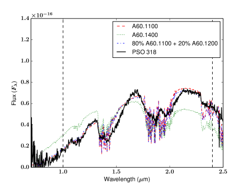
Figure 3.— Top: Best fit single model spectra for model A, AE, and E clouds from Madhusudhan et al. (2011) overlaid on the spectrum of PSO J318.5-22 presented in Liu et al. (2013). The overall best fit model has T_eff=1100 K, log(g)=4, solar metallicity, and model A (thick) clouds. AE and E cloud models fail to reproduce the observed spectrum. Bottomt: T_eff=1400 K, log(g)=4, solar metallicity, and model A (thick) cloud spectrum as well as the best fit multi-component spectrum, consisting of 80$\%$ T_eff=1100 K + 20$\%$ T_eff=1200 K model A clouds overplotted on the Liu et al. (2013) spectrum. Hotter models do not fit the observed features of the Liu et al. (2013) spectrum; the combined 1100 K + 1200 K model spectrum reproduces the observed spectrum marginally better than the best fit single component model.

Figure 4.— top left and top right: predicted K_S to J_S amplitude ratio $A_{K_{S}}/A_{J_{S}}$ as a function of $\Delta$T, the temperature difference between cloud components at T₁ and T₂, and for a filling fraction of the T₂ regions of 0.2. Inhomogeneous cloud cover is plotted on the left (AE+E, A+E, A+AE) and homogeneous cloud cover is plotted on the right (E+E, A+A, AE+AE). The yellow region denotes the values of the amplitude ratio that have previously been found for variable field brown dwarfs. Bottom left and bottom right: maximum change in filling fraction needed to produce the observed amplitude A${}_{J_{S}}$ as a function of $\Delta$T.

References

- Allard et al. (2001) Allard, F., Hauschildt, P. H., Alexander, D. R., Tamanai, A., & Schweitzer, A. 2001, ApJ, 556, 357
- Allard et al. (2012) Allard, F., Homeier, D., & Freytag, B. 2012, Royal Society of London Philosophical Transactions Series A, 370, 2765
- Apai et al. (2013) Apai, D., Radigan, J., Buenzli, E., et al. 2013, ApJ, 768, 121
- Artigau et al. (2009) Artigau, É., Bouchard, S., Doyon, R., & Lafrenière, D. 2009, ApJ, 701, 1534
- Beuzit et al. (2008) Beuzit, J.-L., Feldt, M., Dohlen, K., et al. 2008, Proc. SPIE, 7014, 701418
- Biller et al. (2013) Biller, B. A., Crossfield, I. J. M., Mancini, L., et al. 2013, ApJ, 778, L10
- Bonnefoy et al. (2014) Bonnefoy, M., Marleau, G.-D., Galicher, R., et al. 2014, A&A, 567, L9
- Buenzli et al. (2014) Buenzli, E., Apai, D., Radigan, J., Reid, I. N., & Flateau, D. 2014, ApJ, 782, 77
- Buenzli et al. (2015) Buenzli, E., Saumon, D., Marley, M. S., et al. 2015, ApJ, 798, 127
- Chauvin et al. (2005) Chauvin, G., Lagrange, A.-M., Dumas, C., et al. 2005, A&A, 438, L25
- Gagné et al. (2014) Gagné, J., Lafrenière, D., Doyon, R., Malo, L., & Artigau, É. 2014, ApJ, 783, 121
- Gagné et al. (2015) Gagné, J., Faherty, J. K., Cruz, K. L., et al. 2015, arXiv:1506.07712
- Gillon et al. (2013) Gillon, M., Triaud, A. H. M. J., Jehin, E., et al. 2013, A&A, 555, L5
- Joergens et al. (2013) Joergens, V., Bonnefoy, M., Liu, Y., et al. 2013, A&A, 558, L7
- Lagrange et al. (2010) Lagrange, A.-M., Bonnefoy, M., Chauvin, G., et al. 2010, Science, 329, 57
- Liu et al. (2013) Liu, M. C., Magnier, E. A., Deacon, N. R., et al. 2013, ApJ, 777, L20
- Macintosh et al. (2014) Macintosh, B., Graham, J. R., Ingraham, P., et al. 2014, Proceedings of the National Academy of Science, 111, 12661
- Macintosh et al. (2015) Macintosh, B., Graham, J. R., Barman, T., et al. 2015, arXiv:1508.03084
- Madhusudhan et al. (2011) Madhusudhan, N., Burrows, A., & Currie, T. 2011, ApJ, 737, 34
- Mamajek & Bell (2014) Mamajek, E. E., & Bell, C. P. M. 2014, MNRAS, 445, 2169
- Marois et al. (2008) Marois, C., Macintosh, B., Barman, T., et al. 2008, Science, 322, 1348
- Marois et al. (2010) Marois, C., Zuckerman, B., Konopacky, Q. M., Macintosh, B., & Barman, T. 2010, Nature, 468, 1080
- Metchev et al. (2015) Metchev, S. A., Heinze, A., Apai, D., et al. 2015, ApJ, 799, 154
- Moorwood et al. (1998) Moorwood, A., Cuby, J.-G., & Lidman, C. 1998, The Messenger, 91, 9
- Radigan et al. (2012) Radigan, J., Jayawardhana, R., Lafrenière, D., et al. 2012, ApJ, 750, 105
- Radigan et al. (2014) Radigan, J., Lafrenière, D., Jayawardhana, R., & Artigau, E. 2014, ApJ, 793, 75
- Radigan (2014) Radigan, J. 2014, ApJ, 797, 120
- Saumon & Marley (2008) Saumon, D., & Marley, M. S. 2008, ApJ, 689, 1327
- Snellen et al. (2014) Snellen, I. A. G., Brandl, B. R., de Kok, R. J., et al. 2014, Nature, 509, 63
- Wilson et al. (2014) Wilson, P. A., Rajan, A., & Patience, J. 2014, A&A, 566, A111
- Zapatero Osorio et al. (2006) Zapatero Osorio, M. R., Martín, E. L., Bouy, H., et al. 2006, ApJ, 647, 1405