Modern Monetary Circuit Theory, Stability of Interconnected Banking Network, and Balance Sheet Optimization for Individual Banks

Abstract

A modern version of Monetary Circuit Theory with a particular emphasis on stochastic underpinning mechanisms is developed. It is explained how money is created by the banking system as a whole and by individual banks. The role of central banks as system stabilizers and liquidity providers is elucidated. It is shown how in the process of money creation banks become naturally interconnected. A novel Extended Structural Default Model describing the stability of the Interconnected Banking Network is proposed. The purpose of banks’ capital and liquidity is explained. Multi-period constrained optimization problem for banks’s balance sheet is formulated and solved in a simple case. Both theoretical and practical aspects are covered.

.

Steven Obanno: Do you believe in God, Mr. Le Chiffre?
Le Chiffre: No. I believe in a reasonable rate of return.
Casino Royale

Coffee Cart Man: Hey buddy. You forgot your change.
Joe Moore: [Takes the change] Makes the world go round.
Bobby Blane: What’s that?
Joe Moore: Gold.
Bobby Blane: Some people say love.
Joe Moore: Well, they’re right, too. It is love. Love of gold.
Heist

1 Introduction

Since times immemorial, the meaning of money has preoccupied industrialists, traders, statesmen, economists, mathematicians, philosophers, artists, and laymen alike.

The great British economist John Maynard Keynes puts it succinctly as follows:

For the importance of money essentially flows from it being a link between the present and the future.

These words are echoed by Mickey Bergman, the character played by Danny DeVito in the movie Heist, who says:

Everybody needs money. That’s why they call it money.

Money has been subject of innumerable expositions, see, e.g., Law (1705), Jevons (1875), Knapp (1905), Schlesinger (1914), von Mises (1924), Friedman (1969), Schumpeter (1970), Friedman and Schwartz (1982), Kocherlakota (1998), Realfonzo (1998), Mehrling (2000), Davidson (2002), Ingham (2004), Graeber (2011), McLeay et al. (2014), among many others. Recently, these discussions have been invigorated by the introduction of Bitcoin (Nakamoto 2009). An astute reader will recognize, however, that apart from intriguing technical innovations, Bitcoin does not differ that much from the fabled tally sticks, which were used in the Middle Ages, see, e.g., Baxter (1989). It is universally accepted that money has several important functions, such as a store of value, a means of payment, and a unit of account.

However, it is extraordinary difficult to understand the role played by money and to follow its flow in the economy. One needs to account properly for non-financial and financial stocks (various cumulative amounts), and flows (changes in these amounts). Here is how Michal Kalecki, the great Polish economist, summarizes the issue with his usual flair and penchant for hyperbole:

Economics is the science of confusing stocks with flows.

In our opinion, the functioning of the economy and the role of money is best described by the Monetary Circuit Theory (MCT), which provides the framework for specifying how money lubricates and facilitates production and consumption cycles in society. Although the theory itself is quite established, it fails to include some salient features of the real economy, which came to the fore during the latest financial crisis. The aim of the current paper is to develop a modern continuous time version of this venerable theory, which is capable of dealing with the equality between production and consumption plus investment, the stochastic nature of consumption, which drives other economic variables, defaults of the borrowers, the finite capacity of the banking system for lending, etc. This paper provides a novel description of the behaviour and stability of the interlinked banking system, as well as of the role played by individual banks in facilitating the functioning of the real economy. The latter aspect is particularly important because currently there is a certain lack of appreciation on the part of the conventional economic paradigm of the special role of banks. For example, banks are excluded from widely used dynamic stochastic general equilibrium models, which are presently influential in contemporary macroeconomics (Sbordone et al. 2010).

Some of the key insights on the operation of the economy can be found in Smith (1776), Marx (1867), Schumpeter (1912), Keynes (1936), Kalecki (1939), Sraffa (1960), Minsky (1975, 1986), Stiglitz (1997), Tobin & Golub (1998), Piketty (2014), Dalio (2015), etc. The reader should be cognizant of the fact that opinions of the cited authors very often contradict each other, so that the ”correct” viewpoint on the actual functioning of the economy is not readily discernible.

Monetary Circuit Theory, which can be viewed as a specialized branch of the general economic theory, has a long history. Some of the key historical references are Petty (1662), Cantillon (1755), Quesnay (1759), Jevons (1875). More recently, this theory has been systematically developed by Keen (1995, 2013, 2014) and others. The theory is known under several names such as Stock-Flow Consistent (SFC) Model, Social Accounting Matrix (SAM) Model, etc. Post-Keynsian SFC macroeconomic growth models are discussed in numerous references. Here is a representative selection: Backus et al. (1980), Tobin (1982), Moore (1986, 2006), De Carvalho (1992), Godley (1999), Bellofiore et al. (2000), Parguez and Secareccia (2000), Lavoie (2001, 2004), Lavoie and Godley (2001-2002), Gnos (2003), Graziani (2003), Secareccia (2003), Dos Santos and Zezza (2004, 2006), Zezza & Dos Santos (2004), Godley and Lavoie (2007), Van Treek (2007), Le Heron and Mouakil (2008), Le Heron (2009), Dallery and van Treeck (2011). A useful survey of some recent results is given by Caverzasi and Godin (2013).

It is a simple statement of fact that reasonable people can disagree about the way money is created. Currently, there are three prevailing theories describing the process of money creation. Credit creation theory of banking has been dominant in the 19th and early 20th centuries. It is discussed in a number of books and papers, such as Macleod (1855-6), Mitchell-Innes (1914), Hahn (1920), Wicksell (1922), and Werner (2005). More recently Werner (2014) has empirically illustrated how a bank can individually create money ”out of nothing”. In our opinion, this theory correctly reflects mechanics of linking credit and money creation; unfortunately, it has gradually lost its ground and was overtaken by the fractional reserve theory of banking, see for example, Marshall (1888), Keynes (1930), Samuelson & Nordhaus (1995), and numerous other sources. Finally, the financial intermediation theory of banking is the current champion, three representative descriptions of this theory are given by Keynes (1936), Tobin (1969), and Bernanke & Blinder (1989), among many others. In our opinion, this theory puts insufficient emphasis on the unique and special role of the banking sector in the process of money creation.

In the present paper we analyze the process of money creation and its intrinsic connection to credit in the modern economy. In particular, we address the following important questions: (a) Why do we need banks and what is their role in society? (b) Can a financial system operate without banks? (c) How do banks become interconnected as a part of their regular lending activities? (d) What makes banks different from non-financial institutions? In addition, we consider a number of issues pertinent to individual banks, such as (e) How much capital do banks need? (f) How liquidity and capital are related? (g) How to optimize a bank balance sheet? (h) How would an ideal bank look like? (i) What are the similarities and differences between insurance companies and banks viewed as dividend-producing machines? In order to answer these crucial questions we develop a new Modern Monetary Circuit (MMC) theory, which treats the banking system on three levels: (a) the system as a whole; (b) an interconnected set of individual banks; (c) individual banks. We try to be as parsimonious as possible without sacrificing an accurate description of the modern economy with a particular emphasis on credit channels of money creation in the supply-demand context and their stochastic nature.

The paper is organized as follows. Initially, in Sections 2 and 3 we develop the building blocks, which are further aggregated in Section 4 into the consistent continuous time MMC theory. In Section 2, we introduce stochasticity into conventional Lotka-Volterra-Goodwin equations and incorporate natural restrictions on the relevant economic variables. Further, in Section 3 we analyze the conventional Keen equations and modify them by incorporating stochastic effects and natural boundaries. Building upon the results of Sections 2 and 3, we develop in Section 4 a consistent MMC theory and illustrate it for a simple economic triangle that includes consumers (workers and rentiers), producers and banks. Section 5 details the underlying process of money creation and annihilation by the banking system and discusses the role of the central bank as the liquidity provider for individual banks. In Section 6 we develop the framework to study the banking system, which becomes interlinked in the process of money creation and propose an extended structural default model for the interconnected banking network. This model is further explained in Appendix A for the simple case of two interlinked banks with mutual obligations. In Section 7 the behaviour of individual banks operating as a part of the whole banking system is analyzed with an emphasis on the role of banks’ capital and liquidity. The balance sheet optimization problem for an individual bank is formulated and solved in a simplified case.

2 Stochastic Modified Lotka-Volterra-Goodwin Equations

2.1 Background

The Lotka-Volterra system of first-order non-linear differential equations qualitatively describes the predator-prey dynamics observed in biology (Lotka 1925, Volterra 1931). Goodwin was the first to apply these equations to the theory of economic growth and business cycles (Goodwin 1967). His equations, which establish the relationship between the worker’s share of national income and employment rate became deservedly popular because of their simple and parsimonious nature and ability to provide a qualitative description of the business cycle. However, they do have several serious drawbacks, including their non-stochasticity, prescriptive nature of firms’ investment decisions, and frequent violations of natural restrictions on the corresponding economic variables. Although, multiple extensions of the Goodwin theory have been developed over time (see, e.g., Solow 1990, Franke et al. 2006, Barbosa-Filho and Taylor 2006, Veneziani and Mohun 2006, Desai et al. 2006, Harvie et al. 2007, Kodera and Vosvrda 2007, Taylor 2012, Huu and Costa-Lima 2014, among others), none of them is able of holistically account for all the deficiencies outlined above. In this section we propose a novel mathematically consistent version of the Goodwin equations, which we subsequently use as a building block for the MMC theory described in Section 4.

2.2 Framework

Assume, for simplicity, that in the stylized economy a single good is produced. Then the productivity of labor $\theta_{w}$ is measured in production units per worker per unit of time, the available workforce $N_{w}$ is measured in the number of workers, while the employment rate $\lambda_{w}$ is measured in fractions of one. Thus, the total number of units produced by firms per unit of time, $\Upsilon_{f}$, is given by

$$\Upsilon_{f}=\theta_{w}\lambda_{w}N_{w},$$ (1)

where both productivity and labor pool grow deterministically as

$$\frac{d\theta_{w}}{\theta_{w}}=\alpha dt,$$ (2)

$$\frac{dN_{w}}{N_{w}}=\beta dt.$$ (3)

If so desired, these relations can be made much more complicated, for example, we can add stochasticity, more realistic population dynamics, etc. Production expressed in monetary terms is given by

$$Y_{f}=\theta_{w}\lambda_{w}N_{w}P,$$ (4)

where $P$ is the price of one unit of goods. Similarly to Eqs (2), (3) we assume that the price is deterministic, such that

$$\frac{dP}{P}=\gamma dt.$$ (5)

Workers’ and firms’ share of production are denoted by $s_{w},s_{f}=1-s_{w}$, respectively. The unemployment rate $\lambda_{u}$ is defined in the usual way, $\lambda_{u}=1-\lambda_{w}$. Goodwin’s idea was to describe joint dynamics of the pair $\left(s_{w},\lambda_{w}\right)$.

2.3 Existing Theory

The non-stochastic Lotka-Volterra-Goodwin equations (LVGEs, see Lotka 1925, Volterra 1931, Goodwin 1967), describe the relation between the workers’ portion of the output and the relative employment rate.

The log-change of $s_{w}$ is govern by the Phillips law and can be written in the form

$$\frac{ds_{w}}{s_{w}}=\left(-a+b\lambda_{w}\right)dt\equiv\phi\left(\lambda\right)dt,$$ (6)

where $\phi\left(\lambda\right)$ it the so-called Phillips curve (Phillips 1958, Flaschel 2010, Blanchflower and Oswald 1994).

The log-change of $\lambda_{w}$ is calculated in three easy steps. First, the so-called Cassel-Harrod-Domar (see Cassel 1924, Harrod 1939, Domar 1946) law is used to show that

$$Y_{f}=\nu_{f}K_{f},$$ (7)

where $K_{f}$ is the monetary value of the firm’s non-financial assets and $\nu_{f}$ is the constant production rate, which is the inverse of the capital-to-output ratio $\varpi_{f}$, $\nu_{f}=1/\varpi_{f}$. It is clear that $\nu_{f}$, which can be thought of as a rate, is measured in units of inverse time, $\left[1/T\right]$, while $\varpi_{f}$ is measured in units of time, $\left[T\right]$. Second, Say’s law (Say 1803), which states that all the firms’ profits, given by

$$\Pi_{f}=s_{f}Y_{f}=s_{f}\nu_{f}K_{f},$$ (8)

are re-invested into business, so that the dynamics of $K_{f}$ is govern by the following deterministic equation

$$\frac{dK_{f}}{K_{f}}=\frac{dY_{f}}{Y_{f}}=\left(s_{f}\nu_{f}-\xi_{A}\right)dt,$$ (9)

with $\xi_{A}$ being the amortization rate. Finally, the relative change in employment rate, $\lambda_{w}$ is derived by combining Eqs. (2) - (5) and (9):

$$\frac{d\lambda_{w}}{\lambda_{w}}=\frac{dY_{f}}{Y_{f}}-\frac{d\theta_{w}}{\theta_{w}}-\frac{dN_{w}}{N_{w}}-\frac{dP}{P}=\left(s_{f}\nu_{f}-\alpha-\beta-\gamma-\xi_{A}\right)dt.$$ (10)

Symbolically,

$$\frac{d\lambda_{w}}{\lambda_{w}}=\left(c-ds_{w}\right)dt.$$ (11)

Thus, the coupled system of equations for $\left(s_{w},\lambda_{w}\right)$ has the form

$$\frac{ds_{w}}{s_{w}} = -\left(a-b\lambda_{w}\right)dt,$$ (12)

$$\frac{d\lambda_{w}}{\lambda_{w}} = \left(c-ds_{w}\right)dt.$$

Eqs (12) schematically describe the class struggle; they are formally identical to the famous predator-pray Lotka-Volterra equations in biology, with intensive variables $s_{w},\lambda_{w}$ playing the role of predator and pray, respectively. Two essential drawbacks of the LGVE are that they neglect the stochastic nature of economic processes and do not preserve natural constraints $\left(s_{w},\lambda_{w}\right)\in\left(0,1\right)\times\left(0,1\right)$. Besides, they are too restrictive in describing the discretionary nature of firms’ investment decisions. The conservation law $\Psi$ corresponding Eqs. (12) has the following form

$${\Psi\left(s_{w},\lambda_{w}\right)=-\ln\left(s_{w}^{c}\lambda_{w}^{a}\right)+ds_{w}+b\lambda_{w},}$$ (13)

and has a fixed point at

$$\left(\frac{c}{d},\frac{a}{b}\right),$$ (14)

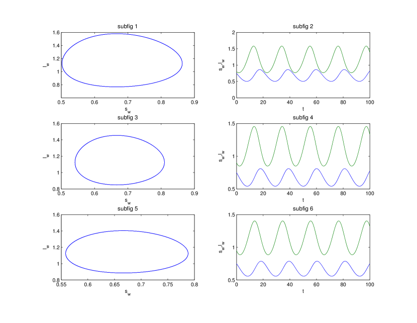
where $\Psi$ achieves its minimum. Solutions of the LVGEs without regularization are shown in Figure 1. Both phase diagrams in the ${\left(s_{w},\lambda_{w}\right)}$-space and time evolution graphs show that for the chosen set of parameters $\lambda_{w}>1$ for some parts of the cycle.

Figure 1 near here.

2.4 Modified Theory

In order to satisfy natural boundaries in the stochastic framework, we propose a new version of the LVGEs of the form

$$ds_{w} = -\left(a-b\lambda_{w}-\frac{\omega}{\lambda_{u}}\right)s_{w}dt+\sigma_{s}\sqrt{s_{w}s_{f}}dW_{s}\left(t\right),$$ (15)

$$d\lambda_{w} = \left(c-ds_{w}-\frac{\omega}{s_{f}}\right)\lambda_{w}dt+\sigma_{\lambda}\sqrt{\lambda_{w}\lambda_{u}}dW_{\lambda}\left(t\right),$$

where $\omega>0$ is a regularization parameter, and $\sigma_{s}\sqrt{s_{w}s_{f}}$, $\sigma_{\lambda}\sqrt{\lambda_{w}\lambda_{u}}$ are Jacobi normal volatilities. This choice of volatilities ensures that ${\left(s_{w},\lambda_{w}\right)}$ stays within the unit square. Deterministic conservation law $\Psi$ for Eqs (15) is similar to Eq. (13):

$${\Psi\left(s_{w},\lambda_{w}\right)=-\ln\left(s_{w}^{c-\omega}s_{f}^{\omega}\lambda_{w}^{a-\omega}\lambda_{u}^{\omega}\right)+ds_{w}+b\lambda_{w}.}$$ (16)

However, it is easy to see that the corresponding contour lines stay within the unit square, $\left(s_{w},\lambda_{w}\right)\in\left(0,1\right)\times\left(0,1\right)$. The fixed point, where $\Psi$ achieves its minimum, is given by

$$\left(\frac{1}{2d}\left(c+d-\sqrt{\left(c-d\right)^{2}+4d\omega}\right),\frac{1}{2b}\left(a+b-\sqrt{\left(a-b\right)^{2}+4b\omega}\right)\right).$$ (17)

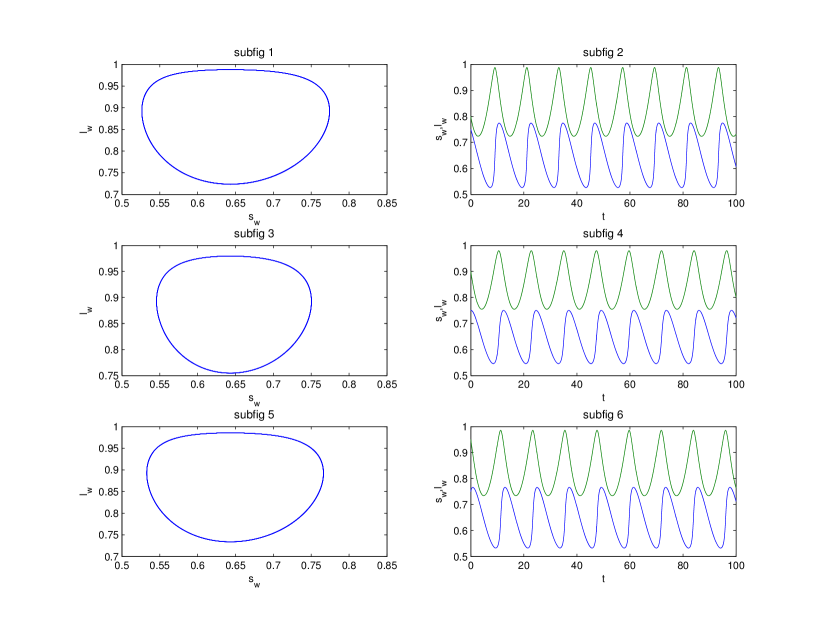
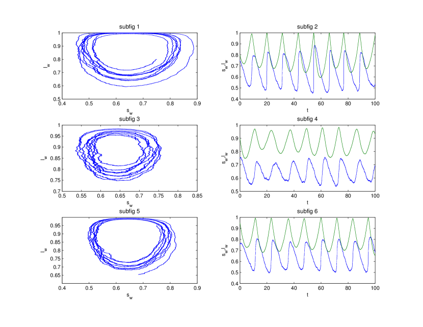
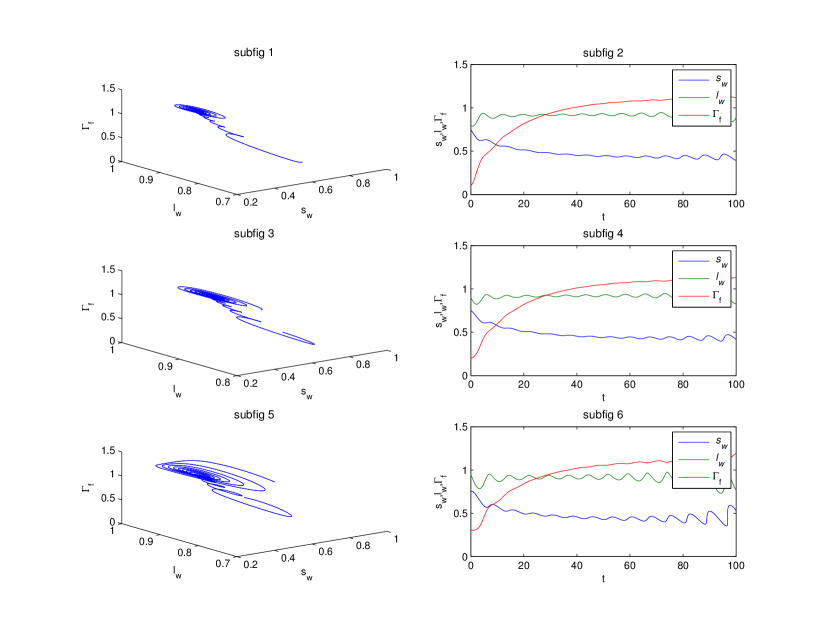
Effects of regularization and effects of stochasticity combined with regularization are shown in Figures 2  and 3, respectively. It is clear that, by construction, Eqs.(15) reflect naturally occurring stochasticity of the corresponding economic processes, while preserving natural bounds for $s_{w}$ and $\lambda_{w}$.

Figure 2 near here.

Figure 3 near here.

The idea of regularizing the Goodwin equations was originally proposed by Desai et al. (2006). Our choice of the regularization function is different from theirs but is particularly convenient for further development and advantageous because of its parsimony. At the same time, while stochastic LVEs are rather popular in the biological context, see, e.g., Cai and Lin (2004), stochastic aspects of the LVGEs remain relatively unexplored, see, however, Kodera and Vosvrda (2007), and, more recently, Huu and Costa-Lima (2014).

3 Stochastic Modified Keen Equations

3.1 Background

LVGEs and their simple modifications generate phase portraits, which are either closed or almost closed, as presented in Figures 1, 2, 3. Accordingly, they can not describe unstable economic behaviour. However, historical experience suggests that capitalist economies are periodically prone to crises, as is elucidated by the famous Financial Instability Hypothesis of Minsky (Minsky 1977, 1986). His theory bridges macroeconomics and finance and, if not fully develops, then, at least clarifies the role of banks and, more generally, debt in modern society. Although Minsky’s own attempts to formulate the theory in a quantitative rather than qualitative form were unsuccessfull, it was partially accomplished by Steven Keen (Keen 1995). Keen extended the Goodwin model by abandoning its key assumption that investment is equal to profit. Instead, he assumed that, when profit rate is high, firms invest more than their retained earnings by borrowing from banks and vice versa.

Below we briefly discuss the Keen equations and show how to modify them in order to remove some of their intrinsic deficiencies.

3.2 Keen Equations

The Keen equations (KEs) (Keen 1995), describe the relation between the workers’ portion of the output $s_{w}$, the employment rate $\lambda_{w}$, and the firms’ debt $D_{f}$ relative to their non-financial assets $K_{f}$, $\Gamma_{f}=D_{f}/K_{f}$. All these quantities are non-dimensional. KEs can be used to provide quantitative description of Minsky’s Financial Instability Hypothesis (Minsky 1977).

Keen expanded the Goodwin framework by abandoning one of its key simplifications, namely, the assumption that investment equals profit. Instead, he allowed investments to be financed by banks. This important extension enables the description of ever increasing firms’ leverage until the point when their debt servicing becomes infeasible and an economic crisis occurs. Subsequently, Keen (2013, 2014) augmented his original equations in order to account for flows of funds among firms, banks, and households. However, KEs and their extensions do not take into account the possibility of default by borrowers, and do not reflect the fact that the banking system’s lending ability is restricted by its capital capacity. Even more importantly, extended KEs do not explicitly guarantee that production equals consumption plus investment. In addition, as with LVGEs, KEs do not reflect stochasticity of the underlying economic behaviour and violate natural boundaries. Accordingly, a detailed description of the crisis in the Keen framework is not possible.

Symbolically, KEs can be written as

$$ds_{w} = -\left(a-b\lambda_{w}\right)s_{w}dt,$$ (18)

$$d\lambda_{w} = \left(\nu_{f}f\left(s_{f}-\frac{r_{L}\Gamma_{f}}{\nu_{f}}\right)-c\right)\lambda_{w}dt,$$

$$d\Gamma_{f} = \left(\left(r_{L}-\nu_{f}f\left(s_{f}-\frac{r_{L}\Gamma_{f}}{\nu_{f}}\right)+d\right)\Gamma_{f}+\nu_{f}\left(f\left(s_{f}-\frac{r_{L}\Gamma_{f}}{\nu_{f}}\right)-s_{f}\right)\right)dt.$$

where $a,b,c,d$ are suitable parameters, and $f\left(.\right)$ is an increasing function of its argument which represents net profits. Keen and subsequent authors recommend the following choice

$$f\left(x\right)=p+\exp\left(qx+r\right).$$ (19)

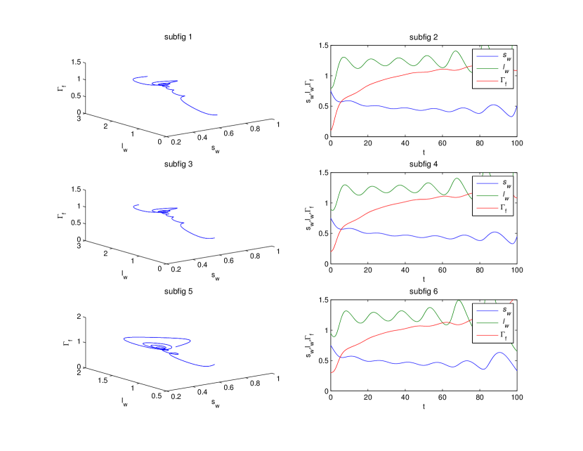
Solutions of KEs without Regularization are shown in Figure 4.

Figure 4 near here.

On the one hand, these figures exhibit the desired features of the rapid growth of firms’ leverage. On the other hand, they produce an unrealistic unemployment rate $\lambda_{w}>1$.

3.3 Modified Theory

A simple modification along the lines outlined earlier, makes KEs more credible:

$$ds_{w} = -\left(a-b\lambda_{w}-\frac{\omega}{\lambda_{u}}\right)s_{w}dt+\sigma_{s}\sqrt{s_{w}s_{f}}dW_{s}\left(t\right),$$ (20)

$$d\lambda_{w} = \left(f\left(s_{f}-\frac{r_{L}\Gamma_{f}}{\nu_{f}}\right)-c-\frac{\omega}{s_{f}}\right)\lambda_{w}dt+\sigma_{\lambda}\sqrt{\lambda_{w}\lambda_{u}}dW_{\lambda}\left(t\right),$$

$$d\Gamma_{f} = \left(\left(r_{L}-\nu_{f}f\left(s_{f}-\frac{r_{L}\Gamma_{f}}{\nu_{f}}\right)+d\right)\Gamma_{f}+\nu_{f}\left(f\left(s_{f}-\frac{r_{L}\Gamma_{f}}{\nu_{f}}\right)-s_{f}\right)\right)dt.$$

Here $\omega$ is a regularization parameter, and $\sigma_{s}\sqrt{s_{w}s_{f}}$, $\sigma_{\lambda}\sqrt{\lambda_{w}\lambda_{u}}$ are Jacobi normal volatilities.

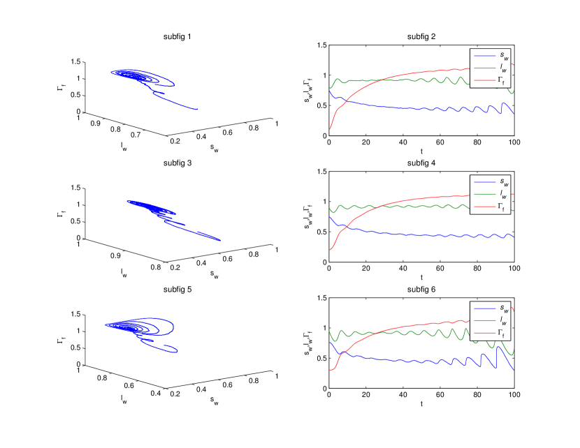
Effects of regularization and effects of stochasticity combined with regularization for KEs are presented in Figures 5  and 6, respectively.

Figure 5 near here.

Figure 6 near here.

While these Figures demonstrate the same rapid growth of firms’ leverage as in Figure 4, while ensuring that $\lambda_{w}<1$, without taking into account a possibility of defaults they are not detailed enough to describe the approach of a crisis and the moment of the crisis itself.

Here and above we looked at the classical LVGEs and KEs and modified them to better reflect the underlying economics. We use these equations as an important building block for the stochastic MMC theory.

4 A Simple Economy: Consumers, Producers, Banks

4.1 Inspiration

Inspired by the above developments, we build a continuous-time stochastic model of the monetary circuit, which has attractive features of the established models, but at the same time explicitly respects the fact that production equals consumption plus investment, incorporate a possibility of default by borrowers, satisfies all the relevant economic constraints, and can be easily extended to integrate the government and central bank, as well as other important aspects, in its framework. For the first time, defaults by borrowers are explicitly incorporated into the model framework.

For the sake of brevity, we shall focus on a reduced monetary circuit consisting of firms, banks, workers, and rentiers, while the extended version will be reported elsewhere.

4.2 Stocks and Flows

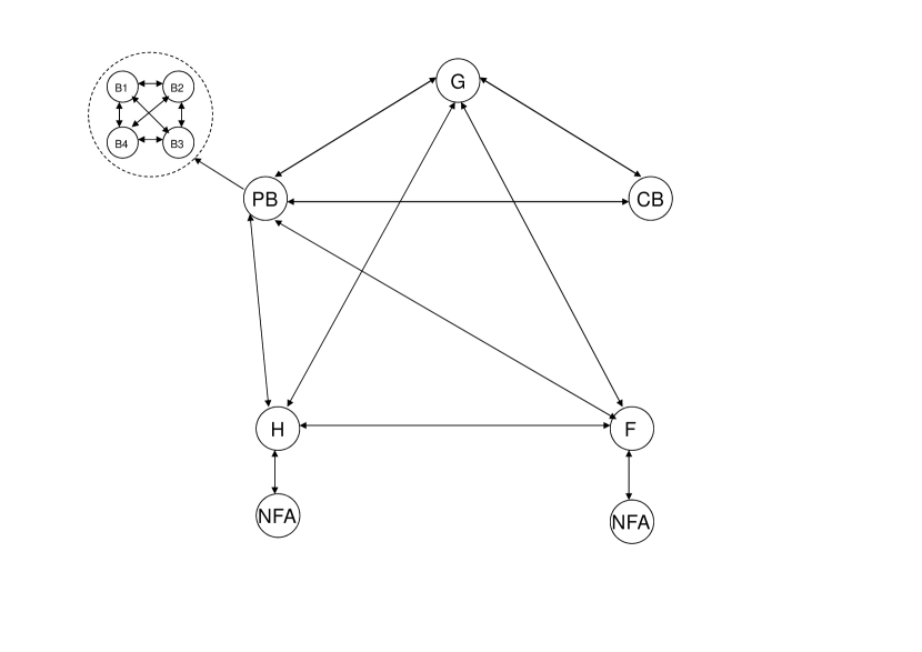
To describe the monetary circuit in detail, we need to consider five sectors: households (workers and rentiers) $H$; firms (capitalists) $F$; private banks (bankers) $PB$; government $G$; and central bank $CB$; all these sectors are presented in Figure 7 below. However, the simplest viable economic graph with just three sectors, namely, households $H$, firms $F$, and private banks $PB$, can produce a nontrivial monetary circuit, which is analyzed below. Banks naturally play a central role in the monetary circuit by simultaneously creating assets and liabilities. However, this crucial function is performed under constraints on banks capital and liquidity. The emphasis on capital and liquidity in the general context of monetary circuits is an important and novel feature, which differentiates our approach from the existing ones. Further details, including the role of the central bank as a system regulator, will be reported elsewhere.

Figure 7 near here.

4.2.1 Notation

We use subscripts $w,r,f,b$ to denote quantities related to workers, rentiers, firms, and banks, respectively. We denote rentiers’ and firms’ deposits (banks’ liabilities) by $D_{r},D_{f}$, and their loans (banks’ assets) by $L_{r},L_{f}$. Firms’ physical, non-financial assets are denoted by $K_{f}$; banks’ capital $K_{b}$; all these quantities are expressed in monetary units, $\left[M\right]$. Thus, financial and nonfinancial stocks are denoted by $D_{r},L_{r},D_{f},L_{f},K_{f},K_{b}$. By its very nature, bank capital, $K_{b}$ is a balancing variable between bank’s assets $(L_{r}+L_{f})$ and liabilities $\left(D_{r}+D_{f}\right)$,

$$K_{b}=L_{r}+L_{f}-\left(D_{r}+D_{f}\right).$$ (21)

According to banking regulations, bank assets are limited by the capital constraints,

$$K_{b}>\nu_{b}\left(L_{r}+L_{f}\right),$$ (22)

where $\nu_{b}$ is a non-dimensional capital adequacy ratio, which defines the overall leverage in the financial system. When dealing with the banking system as a whole, which, in essence can be viewed as a gigantic single bank, we do not need to include the central bank, since the liquidity squeeze cannot occur by definition. It goes without saying that when we deal with a set of individual banks, the introduction of the central bank is an absolute necessity. This extended case will be presented elsewhere.

There are several important rates, which determine monetary flows in our simplified economy, namely, the deposit rate $r_{D}$, loan rate $r_{L}$, maximum production rate at full employment, $v_{f}$, physical assets amortization rate $\xi_{A}$, default rate $\xi_{\Delta}$; all these rates are expressed in terms of inverse time units, $\left[1/T\right]$.

Contractual net interest cash flows for rentiers and firms, $ni_{r,f}$, which are measured in terms of monetary units per time $\left[M/T\right]$, have the form

$$ni_{r,f}=r_{D}D_{r,f}-r_{L}L_{r,f}.$$ (23)

Profits for firms and banks are denoted as $\Pi_{f}$ and $\Pi_{b}$, respectively, with both quantities being expressed in monetary units per time, $\left[M/T\right]$. For future discussion, in addition to the overall profits, we introduce distributed, $\Pi_{f}^{d}$ and $\Pi_{b}^{d}$, and undistributed, $\Pi_{f}^{u}$ and $\Pi_{b}^{u}$, portions of the profits.

It is also necessary to introduce various fractions, some of which we are already familiar with, such as the workers’ share of production $s_{w}$, the firms’ share of production $s_{f}=1-s_{w}$, employment rate $\lambda_{w}$, unemployment rate $\lambda_{u}=1-\lambda_{w}$, and some of which are new, such as capacity utilization $u_{f}$, the rentiers’ share of firms’ profits $\delta_{rf}$, the firms’ share of the firms’s profits $\delta_{ff}=1-\delta_{rf}$, the rentiers’ share of banks’ profits $\delta_{rb}$, the banks’ share of the banks’s profits $\delta_{bb}=1-\delta_{rb}$; all these quantities are non-dimensional, $\left[1\right],$ and sandwiched between 0 and 1. It is clear that $\Pi_{f}^{d}=\delta_{rf}\Pi_{f}$, etc.

4.2.2 Key Observations

(a) Production is equal to consumption plus investment:

$$Y_{f}=C_{w}+C_{r}+I_{f}.$$ (24)

All quantities in Eq. (24) are expressed in terms of $\left[M/T\right].$

(b) On the one hand, the workers’ participation in the system is essentially non-financial and amounts to straightforward exchange of labor for goods, so that

$$C_{w}=s_{w}Y_{f}.$$ (25)

Thus, as was pointed out by Kaletcki, workers consume what they earn.

(c) On the other hand, rentiers can discretionally choose their level of consumption, $C_{r},$ introducing therefore the notion of stochasticity into the picture. We explicitly model the stochastic nature of their consumption by assuming that it is governed by the SDE of the form

$$dC_{r} = \kappa\left(\bar{C}_{r}-C_{r}\right)dt+\sigma C_{r}dW_{C}\left(t\right)$$ (26)

$$\bar{C}_{r} = \alpha_{0}\left(ni_{r}+\Pi_{f}^{d}+\Pi_{b}^{d}\right)+\alpha_{1}\nu_{f}K_{f},$$

where we use the fact that total stock $\Sigma_{r}$ of financial and non-financial assets belonging to rentiers (as a class) is given by

$$\Sigma_{r} = D_{r}-L_{r}+K_{f}+D_{f}-L_{f}+K_{b}$$

$$= D_{r}-L_{r}+K_{f}+D_{f}-L_{f}+L_{r}+L_{f}-D_{r}-D_{f}$$

$$= K_{f}.$$

In other words, the rentiers’ property boils down to firms’ non-financial assets. Eqs (26) assume that rentiers’ consumption is reverting to the mean, $\bar{C}_{r},$ which is a linear combination of profits received by rentiers, $ni_{r}+\Pi_{f}^{d}+\Pi_{b}^{d}$, and the theoretical productivity of their capital, $\nu_{f}K_{f}$.

(d) We apply the celebrated Hooke’s law and assume that firms invest in proportion to their overall production

$$I_{f}=\gamma_{f}Y_{f}$$ (28)

We view this law as a first-order linearization of any hyperelastic relation, which exists in practice. Thus, firms’ production depends on rentiers’ consumption

$$Y_{f}=\frac{C_{r}}{s_{f}-\gamma_{f}},$$ (29)

Here we assume that firms reinvest in production out of the share of their profits, so that $0<\gamma_{f}<s_{f}$, keeping $C_{r}$ positive, $C_{r}>0$. It is convenient to represent $\gamma_{f}$ in the form

$$\gamma_{f}=\upsilon_{f}s_{f},$$ (30)

$0<\upsilon_{f}<1$, and represent $Y_{f}$ in the form

$$Y_{f}=\frac{C_{r}}{\left(1-\upsilon_{f}\right)s_{f}}.$$ (31)

(e) Thus, the level of investment and capacity utilization are given by

$$I_{f}=\frac{\upsilon_{f}C_{r}}{\left(1-\upsilon_{f}\right)},$$ (32)

$$u_{f}=\frac{Y_{f}}{\nu_{f}K_{f}}=\frac{C_{r}}{\left(s_{f}-\gamma_{f}\right)\nu_{f}K_{f}}=\frac{C_{r}}{\left(1-\upsilon_{f}\right)s_{f}\nu_{f}K_{f}}.$$ (33)

(f) Firms’ overall profits, distributed, and undistributed, are defined as

$$\Pi_{f} = s_{f}Y_{f}+r_{D}D_{f}-r_{L}L_{f}=\frac{C_{r}}{\left(1-\upsilon_{f}\right)}+ni_{f},$$ (34)

$$\Pi_{f}^{d} = \delta_{rf}\Pi_{f},\ \ \ \ \ \Pi_{f}^{u}=\delta_{ff}\Pi_{f}.$$

Thus, firms’ profits are directly proportional to rentiers consumption. As usual, Kaletcki put it best by observing that capitalists earn what they spend!

The dimensionless profit rate $\pi_{f}$ is

$$\pi_{f}=\frac{\Pi_{f}}{K_{f}}.$$ (35)

The proportionality coefficient $\upsilon_{f}$ introduced in Eq. (30) depends on the profit rate, capacity utilization, financial leverage, etc., so that

$$\upsilon_{f}=\Phi\left(\upsilon_{0}+\upsilon_{1}\frac{s_{f}Y_{f}}{\nu_{f}K_{f}}+\upsilon_{2}\frac{D_{f}}{K_{f}}+\upsilon_{3}\frac{L_{f}}{K_{f}}\right),$$ (36)

or, explicitly,

$$\upsilon_{f}=\Phi\left(\upsilon_{0}+\upsilon_{1}\frac{C_{r}}{\left(1-\upsilon_{f}\right)\nu_{f}K_{f}}+\upsilon_{2}\frac{D_{f}}{K_{f}}+\upsilon_{3}\frac{L_{f}}{K_{f}}\right),$$ (37)

where $\Phi\left(.\right)$ maps the real axis onto the unit interval, constants $\upsilon_{0},\upsilon_{1},\upsilon_{2}$ are positive, and constant $\upsilon_{3}$ is negative. We choose $\Phi$ in the form

$$\Phi\left(x\right)=\frac{1}{1+\exp\left(-2x\right)}.$$ (38)

(g) Banks’ overall profits, distributed, and undistributed, represent the difference between interest received on outstanding loans and paid on banks deposits reduced by defaults on loans, so that

$$\Pi_{b}=-\xi_{\Delta}\left(L_{r}+L_{f}\right)-ni_{r}-ni_{f},\ \ \ \ \ \Pi_{b}^{d}=\delta_{rb}\Pi_{b},\ \ \ \ \ \Pi_{b}^{u}=\delta_{bb}\Pi_{b}.$$ (39)

(h) Rentiers’ cash flows are

$$CF_{r}=r_{D}D_{r}-r_{L}L_{r}+\ \Pi_{f}^{d}+\ \Pi_{b}^{d}-C_{r}=ni_{r}+\ \Pi_{f}^{d}+\ \Pi_{b}^{d}-C_{r}.$$ (40)

If $CF_{r}>0$, then rentiers’ deposits, $D_{r}$, increase, otherwise, their loans, $L_{r}$, increase. Thus

$$dD_{r}=\left(ni_{r}+\ \Pi_{f}^{d}+\ \Pi_{b}^{d}-C_{r}\right)^{+}dt=\left(CF_{r}\right)^{+}dt,$$ (41)

$$dL_{r} = -\xi_{\Delta}L_{r}dt+\left(-ni_{r}-\ \Pi_{f}^{d}-\ \Pi_{b}^{d}+C_{r}\right)^{+}dt$$

$$= -\xi_{\Delta}L_{r}dt+\left(-CF_{r}\right)^{+}dt.$$

This equation takes into account a possibility of rentiers’ default.

(i) Firms’ cash flows are

$$CF_{f}=\Pi_{f}^{u}-\gamma_{f}Y_{f}.$$ (43)

If $CF_{f}>0$, then firms’ deposits, $D_{f}$, increase, otherwise, their loans, $L_{f}$, increase. Thus

$$dD_{f}=\left(\Pi_{f}^{u}-\gamma_{f}Y_{f}\right)^{+}dt=\left(CF_{f}\right)^{+}dt,$$ (44)

$$dL_{f} = -\xi_{\Delta}L_{f}dt+\left(-\Pi_{f}^{u}+\gamma_{f}Y_{f}\right)^{-}dt$$

$$= -\xi_{\Delta}L_{f}dt+\left(-CF_{f}\right)^{+}dt.$$

The latter equation takes into account a possibility of firms’ default.

(j) Firms’ physical assets growth depends on their investments and the rate of depreciation,

$$dK_{f}=\left(\frac{\upsilon_{f}C_{r}}{1-\upsilon_{f}}-\xi_{A}K_{f}\right)dt.$$ (46)

(k) Banks’ capital growth is determined by their net interest income and the rate of default,

$$dK_{b}=\Pi_{b}^{u}dt=\delta_{bb}\left(-\xi_{\Delta}\left(L_{r}+L_{f}\right)-ni_{r}-ni_{f}\right).$$ (47)

(l) Physical and Financial capacity constraints (at full employment) have the form

$$Y_{f}=\min\left(Y_{f},\nu_{f}K_{f}\right),$$ (48)

$$\left(-CF_{b}\right)^{+}=\left(-CF_{b}\right)^{+}\mathbb{I}_{\nu_{b}\left(L_{r}+L_{f}\right)-K_{b}<0},$$ (49)

$$\left(-CF_{f}\right)^{+}=\left(-CF_{f}\right)^{+}\mathbb{I}_{\nu_{b}\left(L_{r}+L_{f}\right)-K_{b}<0}.$$ (50)

We emphasize this direct parallel between financial and non-financial worlds, with the capital ratio playing the role of a physical capacity constraint.

(m) We use the above observations to derive a modified version of the LVGEs (15). While the first equation describing the dynamics for $s_{w}$ remains unchanged, the second equation for $\lambda_{w}$ becomes

$$d\lambda_{w} = \left(\frac{I_{f}}{\nu_{f}K_{f}}-\alpha-\beta-\xi_{A}\right)\lambda_{w}dt$$

$$= \left(\frac{\upsilon_{f}}{\left(1-\upsilon_{f}\right)}\frac{C_{r}}{\nu_{f}K_{f}}-\alpha-\beta-\xi_{A}\right)\lambda_{w}dt,$$

or, symbolically,

$$d\lambda_{w}=\left(\frac{\upsilon_{f}}{\left(1-\upsilon_{f}\right)}\frac{C_{r}}{\nu_{f}K_{f}}-c\right)\lambda_{w}dt.$$ (52)

(n) By using Eqs (4) and (31), we can express the level of prices, $P$, as a function of rentiers’ consumption, $C_{r}$, employment, $\lambda_{w}$, and other important economic variables. These equations show that

$$\frac{C_{r}}{\left(1-\upsilon_{f}\right)s_{f}}=\lambda_{w}\theta_{w}N_{w}P.$$ (53)

Accordingly, we can represent $P$ as follows

$$P=\frac{C_{r}}{\left(1-\upsilon_{f}\right)s_{f}\lambda_{w}\theta_{w}N_{w}}.$$ (54)

4.3 Main Equations

In this section we summarize the main dynamic MMC equations and the corresponding constraints

$$\begin{array}[]{l}dC_{r}=\kappa_{C}\left(\bar{C}_{r}-C_{r}\right)dt+\sigma_{C}C_{r}dW_{C}\left(t\right),\\ dD_{r}=\left(\delta_{bb}ni_{r}+\left(\delta_{rf}-\delta_{rb}\right)ni_{f}-\delta_{rb}\xi_{\Delta}\left(L_{r}+L_{f}\right)-\frac{\left(\delta_{ff}-\upsilon_{f}\right)C_{r}}{\left(1-\upsilon_{f}\right)}\right)^{+}dt,\\ dL_{r}=\left(-\xi_{\Delta}L_{r}+\left(-\delta_{bb}ni_{r}-\left(\delta_{rf}-\delta_{rb}\right)ni_{f}+\delta_{rb}\xi_{\Delta}\left(L_{r}+L_{f}\right)+\frac{\left(\delta_{ff}-\upsilon_{f}\right)C_{r}}{\left(1-\upsilon_{f}\right)}\right)^{+}\right)dt,\\ dD_{f}=\left(\delta_{ff}ni_{f}+\frac{\left(\delta_{ff}-\upsilon_{f}\right)C_{r}}{\left(1-\upsilon_{f}\right)}\right)^{+}dt,\\ dL_{f}=\left(-\xi_{\Delta}L_{f}+\left(-\delta_{ff}ni_{f}-\frac{\left(\delta_{ff}-\upsilon_{f}\right)C_{r}}{\left(1-\upsilon_{f}\right)}\right)^{+}\right)dt,\\ dK_{f}=\left(\frac{\upsilon_{f}C_{r}}{\left(1-\upsilon_{f}\right)}-\xi_{A}K_{f}\right)dt+\sigma_{K}K_{f}dW_{K}\left(t\right),\\ dK_{b}=-\delta_{bb}\left(\xi_{\Delta}\left(L_{r}+L_{f}\right)+ni_{r}+ni_{f}\right),\end{array}$$ (55)

where

$$\begin{array}[]{l}ni_{r,f}=r_{D}D_{r,f}-r_{L}L_{r,f},\\ \ \ \bar{C}_{r}=\alpha_{0}\left(\delta_{bb}ni_{r}+\left(\delta_{rf}-\delta_{rb}\right)ni_{f}+\frac{\delta_{rf}C_{r}}{\left(1-\upsilon_{f}\right)}\right)+\alpha_{1}\nu_{f}K_{f},\\ \ \ \ \upsilon_{f}=\Phi\left(\upsilon_{0}+\upsilon_{1}\frac{C_{r}}{\left(1-\upsilon_{f}\right)\nu_{f}K_{f}}+\upsilon_{2}\frac{D_{f}}{K_{f}}+\upsilon_{3}\frac{L_{f}}{K_{f}}\right).\end{array}$$ (56)

The coefficient $\upsilon_{f}$ introduced in Eq. (30) can be found either via the Newton-Raphson method or via fixed-point iteration. The first iteration is generally sufficient, so that, approximately,

$$\upsilon_{f}\approx\Phi\left(\upsilon_{0}+\upsilon_{1}\frac{C_{r}}{\left(1-\Phi\left(\upsilon_{0}\right)\right)\nu_{f}K_{f}}+\upsilon_{2}\frac{D_{f}}{K_{f}}+\upsilon_{3}\frac{L_{f}}{K_{f}}\right).$$ (57)

The physical and financial capacity constraints are

$$\begin{array}[]{l}\ \ \ \ \ \ \ \ \ \ \ Y_{f}=\min\left(Y_{f},\nu_{f}K_{f}\right),\\ \left(-CF_{b}\right)^{+}=\left(-CF_{b}\right)^{+}\mathbb{I}_{\nu_{b}\left(L_{r}+L_{f}\right)-K_{b}<0},\\ \left(-CF_{f}\right)^{+}=\left(-CF_{f}\right)^{+}\mathbb{I}_{\nu_{b}\left(L_{r}+L_{f}\right)-K_{b}<0}.\end{array}$$ (58)

In addition,

$$\begin{array}[]{l}\ d\theta_{w}=\alpha\theta_{w}dt,\\ dN_{w}=\beta N_{w}dt,\\ \ ds_{w}=-\left(a-b\lambda_{w}-\frac{\omega}{\lambda_{u}}\right)s_{w}dt+\sigma_{s}\sqrt{s_{w}s_{f}}dW_{s}\left(t\right),\\ d\lambda_{w}=\left(\frac{\upsilon_{f}C_{r}}{\left(1-\upsilon_{f}\right)\nu_{f}K_{f}}-c-\frac{\omega}{s_{f}}\right)\lambda_{w}dt+\sigma_{\lambda}\sqrt{\lambda_{w}\lambda_{u}}dW_{\lambda}\left(t\right),\\ \ \ \ P=\frac{C_{r}}{\left(1-\upsilon_{f}\right)s_{f}\lambda_{w}\theta_{w}N_{w}}.\end{array}$$ (59)

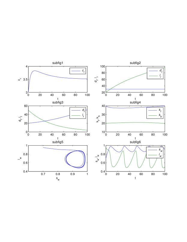
In summary, we propose the closed system of stochastic scale invariant MMC equations (55), (56). By construction, these equation preserve the equality among production and consumption plus investment. In addition, it turns out modified LVGEs play only an auxiliary role and are not necessary for understanding the monetary circuit at the most basic level. This intriguing property is due to the assumption that investments as driven solely by profits. If capacity utilization is incorporated into the picture, then MMC equations and LVGEs become interlinked.

Representative solution of MMC equations is shown in Figure 8.

Figure 8 near here.

5 Money Creation and Annihilation in Pictures

In modern society, where large quantities of money have to be deposited in banks, banks play a unique role as record keepers. Depositors become, in effect, unsecured junior creditors of banks. If a bank were to default, it would generally cause partial destruction of deposits. To avoid such a disturbing eventuality, banks are required to keep sufficient capital cushions, as well as ample liquidity. In addition, deposits are insured up to a certain threshold. Without diving into nuances of different takes on the nature of banking, we mention several books and papers written over the last century, which reflect upon various pertinent issues, such as Schumpeter (1912), Howe (1915), Klein (1971), Saving (1977), Sealey and Lindley (1977), Diamond and Dybvig (1983), Fama (1985), Selgin and White (1987), Heffernan (1996), FRB (2005), Wolf (2014).

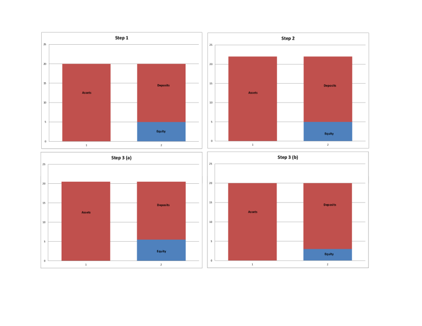
It is very useful to have a simplified pictorial representation for the inner working of the banking system. We start with a simple case of a single bank, or, equivalently, the banking system as a whole. We assume that the bank in question does not operate at full capacity, so that condition (22) is satisfied. If a new borrower, who is deemed to be credit worthy, approaches the bank and asks for a reasonably-sized loan, then the bank issues the loan by simultaneously creating on its books a deposit (the borrower’s asset), and a matching liability for the borrower (the bank’s asset). Figuratively speaking, the bank has created money ”out of thin air”. Of course, when the loan is repaid, the process is carried in reverse, and the money is ”destroyed”. Assuming that the interest charged on loans is greater than the interest paid on deposits, as a result of the round-trip process bank’s capital increases. The whole process, which is relatively simple, is illustrated in Figure 9. At first, the bank has 20 units of assets, 15 units of liabilities, and 5 units of equity. Then, it lends 2 units to a credit worthy borrower. Now it has 22 units of assets and 17 units of liabilities. Thus, 2 units of new money are created. If the borrower repays her debt with interest, as shown in Step 3(a), then the bank accumulates 20.5 units of assets, 15 units of liabilities, and 5.5 units of equity. If the borrower defaults, as shown in Step 3(b), then the bank ends up with 20 units of assets, 17 units of liabilities, and 3 units of equity. In both cases 2 units of money are destroyed.

Figure 9 near here.

Werner executed this process step by step and described his experiences in a recent paper (Werner 2014). It is worth noting, that in the case of a single bank, lending activity is limited by bank’s capital capacity only and liquidity is not important.

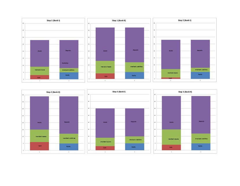
We now consider a more complicated case of two (or, possibly, more) banks. In this case, it is necessary to incorporate liquidity into the picture. To this end, we also must include a central bank into the financial ecosystem. We assume that banks keep part of their assets in cash, which represents a liability of the central bank. The money creation process comprises of three stages: (a) A credit worthy borrower asks the first bank for a loan, which the bank grants out of its cash reserves, thus reducing its liquidity below the desired level; (b) The borrower then deposits the money with the second bank, which converts this deposit into cash, thereby increasing its liquidity above its desired level; (c) The first bank approaches the second bank in order to borrow its excess cash. If the second bank deems the first bank credit worthy, it will lend its excess cash, in consequence creating  a link between itself and the first bank. Alternatively, if the second bank refuses to lend its excess cash to the first bank, the first bank has to borrow funds from the central bank, by using its performing assets as collateral. Thus, the central bank lubricates the wheels of commerce by providing liquidity to credit worthy borrowers. Its willingness to lend money to commercial banks, determines in turn their willingness to lend to firms and households. When the borrower repays its loan the process plays in reverse.

The money creation process, initiated when Bank I lends 2 monetary units to a new borrower, results in the following changes in two banks’ balance sheets:

$$\begin{array}[]{c}\\ \\ \text{External\ Assets}\\ \text{Interbank\ Assets}\\ \text{Cash}\\ \text{External\ Liabilities}\\ \text{Interbank\ Liabilities}\\ \text{Equity}\end{array}\begin{array}[]{cc}\text{Step}&\text{I}\\ \text{Bank\ I}&\text{Bank\ II}\\ 19&24\\ 6&9\\ 3&4\\ 20&25\\ 3&7\\ 5&5\end{array}\begin{array}[]{cc}\text{Step}&\text{II}\\ \text{Bank\ I}&\text{Bank\ II}\\ 21&24\\ 6&9\\ 1&6\\ 20&27\\ 3&7\\ 5&5\end{array}\begin{array}[]{cc}\text{Step}&\text{III}\\ \text{Bank\ I}&\text{Bank\ II}\\ 21&24\\ 6&11\\ 3&4\\ 20&27\\ 5&7\\ 5&5\end{array}$$ (60)

This process is illustrated in Figure 10. We leave it to the reader to analyze the money annihilation process.

Figure 10 near here.

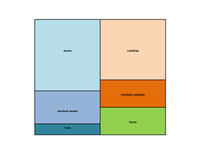
In summary, in contrast to a non-banking firm, whose balance sheet can be adequately described by a simple relationship among assets, $A$, liabilities, $L$, and equity, $E$,

$$A=L+E,$$ (61)

as is shown in Figure 11a, the balance sheet of a typical commercial bank must, in addition to external assets and liabilities, incorporate more details, such as interbank assets and liabilities, as well as cash, representing simultaneously bank’s assets and central bank’s liabilities, see Figure 11b.

Figure 11 near here.

In Section 4 we quantitatively described a supply and demand driven economic system. In this system money is treated on a par with other goods, and the dynamics of demand for loans and lending activity is understood in the supply-demand equilibrium framework. An increasing demand for loans from firms and households leads banks to lend more. Having said that, we should emphasize that the ability of banks to generate new loans is not infinite. In exact parallel with physical goods, whose overall production at full employment is physically limited by $\nu_{f}K_{f}$, the process of money (loan) creation is limited by the capital capacity of the banking system $K_{b}/\nu_{b}$. Once we have embedded the flow of money in the supply-demand framework, we can extend the model to several interconnected banks that issue loans in the economy. These banks compete with each other for business, while, at the same time, help each other to balance their cash holdings thus creating interbank linkages. These linkages are posing risks because of potential propagation of defaults in the system. Our main goal in the next section is to develop a parsimonious model which, nevertheless, is rich enough to produce an adequate quantitative description of the banking ecosystem. We look for a model with as few adjustable parameters as possible rather than one over-fitted with a plethora of adjustable calibration parameters.

6 Interlinked Banking System

Consider $N$ banks with external as well as mutual assets and liabilities of the form

$$A_{i}+\mathop{\displaystyle\sum}\limits_{j\neq i}L_{ji}=A_{i}+\hat{A}_{i}\text{ and }L_{i}+\mathop{\displaystyle\sum}\limits_{j\neq i}L_{ij}=L_{i}+\hat{L}_{i},\ \ i,j=1,...,N,$$ (62)

where the interbank assets and liabilities are defined as

$$\hat{A}_{i}=\mathop{\displaystyle\sum}\limits_{j\neq i}L_{ji},\ \ \ \ \ \hat{L}_{i}=\mathop{\displaystyle\sum}\limits_{j\neq i}L_{ij}.$$ (63)

Accordingly, an individual bank’s capital is given by

$$E_{i}=A_{i}+\hat{A}_{i}-L_{i}-\hat{L}_{i}.$$ (64)

We can represent banks assets and liabilities by using the following asset and liability matrices

$$\begin{array}[]{c}\mathbb{A}=\left(A_{ij}\right),\ \ \ A_{ii}=A_{i},\ \ \ A_{ij}=L_{ji},\\ \mathbb{L=}\left(L_{ij}\right),\ \ \ L_{ii}\equiv L_{i},\ \ \ i,j=1,...,N.\end{array}$$ (65)

Thus, by its very nature banking system becomes inherently linked. Various aspects of this interconnectivity are discussed by Rochet and Tirole (1996), Freixas et al. (2000), Pastor-Satorras and Vespignani (2001), Leitner (2005), Egloff et al. (2007), Allen and Babus (2009), Wagner (2010), Haldane and May (2011), Steinbacher et al. (2014), Ladley (2013), Hurd (2015), among many others.

In the following subsection we specify dynamics for asset and liabilities, which is consistent with a possibility of defaults by borrowers. 

6.1 Dynamics of Assets and Liabilities. Default Boundaries

In the simplest possible case, the dynamics of assets and liabilities is governed by the system of SDEs of the form

$$\frac{dA_{i}\left(t\right)}{A_{i}\left(t\right)}=\mu dt+\sigma_{i}dW_{i}\left(t\right),\ \ \ \frac{dL_{i}\left(t\right)}{L_{i}\left(t\right)}=\mu dt,\ \ \ \frac{dL_{ij}\left(t\right)}{L_{ij}\left(t\right)}=\mu dt.$$ (66)

where $\mu$ is growth rate, not necessarily risk neutral, $W_{i}$ are correlated Brownian motions, and $\sigma_{i}$ are corresponding log-normal volatilities.

In a more general case, the corresponding dynamics can contain jumps, as discussed in Lipton and Sepp (2009), or Itkin and Lipton (2015a, 2015b). Following Lipton and Sepp (2009), we assume that dynamics for firms’ assets is given by

$$\frac{dA_{i}\left(t\right)}{A_{i}\left(t\right)}=\left(\mu-\kappa_{i}\lambda_{i}\left(t\right)\right)dt+\sigma_{i}dW_{i}\left(t\right)+\left(e^{J_{i}}-1\right)dN_{i}\left(t\right),$$ (67)

where $N_{i}$ are Poisson processes independent of $W_{i}$, $\lambda_{i}$ are intensities of jump arrivals, $J_{i}$ are random jump amplitudes with probability densities $\varpi_{i}\left(j\right)$, and $\kappa_{i}$ are jump compensators,

$$\kappa_{i}=\mathbb{E}\left\{e^{J_{i}}-1\right\}.$$ (68)

Since we are interested in studying consequences of default, it is enough to assume that $J_{i}$ are negative exponential jumps, so that

$$\varpi_{i}\left(j\right)=\left\{\begin{array}[]{cc}0,&j>0,\\ \vartheta_{i}e^{\vartheta_{i}j}&j\leq 0,\end{array}\right.$$ (69)

with $\vartheta_{i}>0$. Diffusion processes $W_{i}$ are correlated in the usual way,

$$dW_{i}\left(t\right)dW_{j}\left(t\right)=\rho_{ij}dt.$$ (70)

Jump processes $N_{i}$ are correlated in the spirit of Marshall-Olkin (1967). We denote by $\Pi^{\left(N\right)}$ the set of all subsets of $N$ names except for the empty subset $\left\{\varnothing\right\}$, and by $\pi$ a typical subset. With every $\pi$ we associate a Poisson process $N_{\pi}\left(t\right)$ with intensity $\lambda_{\pi}\left(t\right)$. Each $N_{i}\left(t\right)$ is projected on $N_{\pi}\left(t\right)$ as follows

$$N_{i}\left(t\right)=\sum_{\pi\in\Pi^{\left(N\right)}}1_{\left\{i\in\pi\right\}}N_{\pi}\left(t\right),$$ (71)

with

$$\lambda_{i}\left(t\right)=\sum_{\pi\in\Pi^{\left(N\right)}}1_{\left\{i\in\pi\right\}}\lambda_{\pi}\left(t\right).$$ (72)

Thus, for each bank we assume that there are both systemic and idiosyncratic sources of jumps. In practice, it is sufficient to consider $N+1$ subsets of $\Pi^{\left(N\right)}$, namely, the subset containing all names, and subsets containing only one name at a time. For all other subsets we put $\lambda_{\pi}=0$. If extra risk factors are needed, one can include additional subsets representing particular industry sectors or countries.

The simplest way of introducing default is to follow Merton’s idea (Merton 1974) and to consider the process of final settlement at time $t=T$, see, e.g., Webber and Willison (2011). However, given the highly regulated nature of the banking business, it is hard to justify such a set-up. Accordingly, we prefer to model the problem in the spirit of Black and Cox (1976) and introduce continuous default boundaries, $\Lambda_{i}$, for $0\leq t\leq T$, which are defined as follows

$$A_{i}\leq\Lambda_{i}=\left\{\begin{array}[]{cc}R_{i}\left(L_{i}+\hat{L}_{i}\right)-\hat{A}_{i}\equiv\Lambda_{i}^{<},&\ t<T,\\ L_{i}+\hat{L}_{i}-\hat{A}_{i}\equiv\Lambda_{i}^{=},&t=T,\end{array}\right.$$ (73)

where $R_{i},0\leq R_{i}\leq 1$ is the recovery rate. We can think of $\Lambda_{i}$ as a function of external and mutual liabilities, $\mathbb{L=\{}L_{i},\hat{L}_{i}\}$, $\Lambda_{i}$=$\Psi_{i}\left(\mathbb{L}\right)$.

If the $k$-th bank defaults at an intermediate time $t^{\prime}$, then the capital of the remaining banks is depleted. We change indexation of the surviving banks by applying the following function

$$i\rightarrow i^{\prime}=\phi^{k}\left(i\right)=\left\{\begin{array}[]{ll}i,&i<k,\\ i-1&i>k.\end{array}\right.$$ (74)

We also introduce the inverse function $\psi^{k}$,

$$i\rightarrow i^{\prime}=\psi^{k}\left(i\right)=\left\{\begin{array}[]{ll}i,&i<k,\\ i+1&i\geq k.\end{array}\right.$$ (75)

The corresponding asset and liability matrices $\mathbb{A}^{\left(k\right)}$, $\mathbb{L}^{\left(k\right)}$ assume the form

$$\begin{array}[]{c}\mathbb{A}^{\left(k\right)}=\left(A_{ij}^{\left(k\right)}\left(t\right)\right),\ \ \ A_{ii}^{\left(k\right)}\left(t\right)=A_{\psi^{k}\left(i\right)}\left(t\right),\\ A_{ij}^{\left(k\right)}\left(t\right)=A_{\psi^{k}\left(j\right),\psi^{k}\left(i\right)}\left(t\right),\\ \mathbb{L}^{\left(k\right)}=\left(L_{ij}^{\left(k\right)}\left(t\right)\right),\ \ \ L_{ii}^{\left(k\right)}\left(t\right)=L_{\psi^{k}\left(i\right)}\left(t\right)-L_{\psi^{k}\left(i\right),k}\left(t^{\prime}\right)+R_{k}L_{k,\psi^{k}\left(i\right)}\left(t^{\prime}\right),\\ L_{ij}^{\left(k\right)}\left(t\right)=L_{\psi^{k}\left(i\right),\psi^{k}\left(i\right)}\left(t\right),\\ t>t^{\prime}\text{,\ \ \ }i,j=1,...,N-1.\end{array}$$ (76)

The corresponding default boundaries are given by

$$A_{i}\leq\Lambda_{i}^{\left(k\right)}=\left\{\begin{array}[]{cc}R_{\psi^{k}\left(i\right)}\left(L_{i}^{\left(k\right)}+\hat{L}_{i}^{\left(k\right)}-\hat{A}_{i}^{\left(k\right)}\right),&t<T,\\ L_{i}^{\left(k\right)}+\hat{L}_{i}^{\left(k\right)}-\hat{A}_{i}^{\left(k\right)},&t=T.\end{array}\right.$$ (77)

$i\neq j$. It is clear that

$$\Delta\Lambda_{i}^{\left(k\right)}=\Lambda_{i}^{\left(k\right)}-\Lambda_{i}=\left\{\begin{array}[]{cc}\left(1-R_{i}R_{k}\right)\hat{A}_{i}^{\left(k\right)},&t<T,\\ \left(1-R_{k}\right)\hat{A}_{i}^{\left(k\right)},&t=T.\end{array}\right.$$ (78)

so that $\Delta\Lambda_{i}^{\left(k\right)}>0$ and the default boundaries (naturally) move to the right.

6.2 Terminal Settlement Conditions

In order to formulate the terminal condition for the Kolmogorov equation, we need to describe the settlement process at $t=T$ in the spirit of Eisenberg and Noe (2001). Let $\vec{A}\left(T\right)$ be the vector of the terminal external asset values. Since at time $T$ a full settlement is expected, we assume that a particular bank will pay a fraction $\omega_{i}$ of its total liabilities to its creditors (both external and inter-banks). If its assets are sufficient to satisfy its obligations, then $\omega_{i}=1$, otherwise $0<\omega_{i}<1$. Thus, the settlement  can be described by the following system of equations

$$\min\left(A_{i}\left(T\right)+\mathop{\displaystyle\sum}\limits_{j}L_{ji}\omega_{j},L_{i}+\hat{L}_{i}\right)=\omega_{i}\left(L_{i}+\hat{L}_{i}\right),$$ (79)

or equivalently

$$\Phi_{i}\left(\vec{\omega}\right)\equiv\min\left(\frac{A_{i}\left(T\right)+\mathop{\displaystyle\sum}\limits_{j}L_{ji}\omega_{j}}{L_{i}+\hat{L}_{i}},1\right)=\omega_{i}.$$ (80)

It is clear that $\vec{\omega}$ is a fixed point of the mapping $\vec{\Phi}\left(\vec{\omega}\right)$,

$$\vec{\Phi}\left(\vec{\omega}\right)=\vec{\omega}.$$ (81)

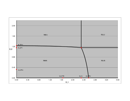
Eisenberg and Noe have shown that $\vec{\Phi}\left(\vec{\omega}\right)$ is a non-expanding mapping in the standard Euclidean metric, and formulated conditions under which there is just one fixed point. We assume that these conditions are satisfied, so that for each $\vec{A}\left(T\right)$ there is a unique $\vec{\omega}\left(\vec{A}\left(T\right)\right)$ such that the settlement is possible. There are no defaults provided that $\vec{\omega}=\vec{1}$, otherwise some banks default. Let $\vec{I}$ be a state indicator $\left(0,1\right)$ vector of length $N$. Denote by $\mathcal{D}\left(\vec{I}\right)$ the following domain

$$\mathcal{D}\left(\vec{I}\right)=\left\{\left.\vec{A}\left(T\right)\right|\omega_{i}\left(\vec{A}\left(T\right)\right)=\left\{\begin{array}[]{cc}1,&I_{i}=1\\ <1&I_{i}=0\end{array}\right.\right\}.$$ (82)

In this domain the $i$-th bank survives provided that $I_{i}=1$, and defaults otherwise. For example in the domain $\mathcal{D}\left(1,...,1\right)$ all banks survive, while in the domain $\mathcal{D}\left(0,1,...,1\right)$ the first bank defaults while all other survive, etc.

The actual terminal condition depends on the particular instrument under consideration. If we are interested in the survival probability $Q$ of the entire set of banks, we have

$$Q\left(T,\vec{A}\right)=1_{\vec{A}\in\mathcal{D}\left(1,...,1\right)}.$$ (83)

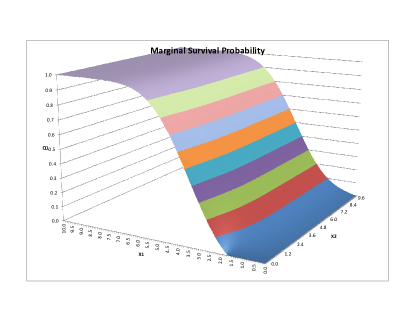
For the marginal survival probability of the $i$-th bank we have

$$Q\left(T,\vec{A}\right)=1_{\vec{A}\in\cup_{\vec{I}^{\left(i\right)}}\mathcal{D}\left(\vec{I}^{\left(i\right)}\right)},$$ (84)

where $\vec{I}^{\left(i\right)}$ is the set of indicator vectors with $I_{i}=1$.

Thus far, we have introduced the stochastic dynamics for assets and liabilities for a set of interconnected banks. These dynamics explicitly allows for defaults of individual banks. Our framework reuses heavy machinery originally developed in the context of credit derivatives. In spite of being mathematical intense, such an approach is necessary to quantitatively describe the financial sector as a manufacturer of credit.

6.3 General Solution via Green’s Function

This Section is rather challenging mathematically and can easily be skipped at first reading.

Our goal is to express general quantities of interest such as marginal survival probabilities for individual banks and their joint survival probability in terms of Green’s function for the $N$-dimensional correlated jump-diffusion process in a positive ortant.

As usual, it is more convenient to introduce normalized non-dimensional variables. To this end, we define

$$\bar{t}=\Sigma^{2}t,\ \ \ \ X_{i}=\frac{\Sigma}{\sigma_{i}}\ln\left(\frac{A_{i}}{\Lambda_{i}^{<}}\right),\ \ \ \ \bar{\lambda}_{i}=\frac{\lambda_{i}}{\Sigma^{2}},$$ (85)

where

$$\Sigma=\left(\mathop{\displaystyle\prod}\limits_{i=1}^{N}\sigma_{i}\right)^{1/N}.$$ (86)

Thus,

$$t=\frac{\bar{t}}{\Sigma^{2}},\ \ \ \ A_{i}=\left(R_{i}\left(L_{i}+\hat{L}_{i}\right)-\hat{A}_{i}\right)e^{\sigma_{i}X_{i}/\Sigma}.$$ (87)

The scaled default boundaries have the form

$$X_{i}\leq M_{i}\left(t\right)=\left\{\begin{array}[]{cc}0\equiv M_{i}^{<},&t<T,\\ \frac{\Sigma}{\sigma_{i}}\ln\left(\frac{L_{i}\left(0\right)+\hat{L}_{i}\left(0\right)-\hat{A}_{i}\left(0\right)}{R_{i}\left(L_{i}\left(0\right)+\hat{L}_{i}\left(0\right)\right)-\hat{A}_{i}\left(0\right)}\right)\equiv M_{i}^{=},&t=T.\end{array}\right.$$ (88)

The survival domain $\mathcal{D}\left(1,...,1\right)$ is given by

$$\mathcal{D}\left(1,...,1\right)=\left\{X_{i}>M_{i}^{=}\right\},$$ (89)

Thus, we need to perform all our calculations in the positive cone $R_{+}^{\left(N\right)}$.

The dynamics of $\vec{X}=\left(X_{1},...,X_{N}\right)$ is governed by the following equations

$$dX_{i} = -\left(\frac{\sigma_{i}}{2\Sigma}+\kappa_{i}\ \bar{\lambda}_{i}\right)d\bar{t}+dW_{i}\left(\bar{t}\right)+\frac{\Sigma}{\sigma_{i}}J_{i}dN_{i}\left(\bar{t}\right)$$

$$\equiv \xi_{i}d\bar{t}+dW_{i}\left(\bar{t}\right)+\zeta_{i}J_{i}dN_{i}\left(\bar{t}\right).$$

Below we omit bars for the sake of brevity and rewrite Eq. (6.3) in the form:

$$dX_{i}=\xi_{i}dt+dW_{i}\left(t\right)+\zeta_{i}J_{i}dN_{i}\left(t\right),$$ (91)

The corresponding Kolmogorov backward operator has the form

$$\mathcal{L}^{\left(N\right)}f = \mathop{\displaystyle\sum}\limits_{i=1}^{N}\left(\frac{1}{2}\mathop{\displaystyle\sum}\limits_{j=1}^{N}\rho_{ij}f_{X_{i}X_{j}}+\xi_{i}f_{X_{i}}\right)$$

$$+\mathop{\textstyle\sum}\limits_{\pi\in\Pi^{\left(N\right)}}\lambda_{\pi}\prod\limits_{i\in\pi}\mathcal{J}_{i}f\left(\vec{X}\right)-\mathop{\textstyle\sum}\limits_{\pi\in\Pi^{\left(N\right)}}\lambda_{\pi}f\left(\vec{X}\right)$$

$$\equiv \frac{1}{2}\Delta_{\rho}f+\xi\cdot\nabla f+\mathcal{J}f-\upsilon f,$$

where

$$\mathcal{J}\left(\vec{X}\right)\mathcal{=}\mathop{\textstyle\sum}\limits_{\pi\in\Pi^{\left(N\right)}}\lambda_{\pi}\prod\limits_{i\in\pi}\mathcal{J}_{i}f\left(\vec{X}\right),$$ (93)

$$\mathcal{J}_{i}f\left(\vec{X}\right)=\varsigma_{i}\int_{0}^{X_{i}}f\left(X_{1},...,X_{i}-j,...X_{N}\right)e^{-\varsigma_{i}j}dj,$$ (94)

and $\varsigma_{i}=\sigma_{i}\vartheta_{i}/\Sigma$.

We can formulate a typical pricing equation in the positive cone $R_{+}^{\left(N\right)}$. We have

$$\partial_{t}V\left(t,\vec{X}\right)+\mathcal{L}^{\left(N\right)}V\left(t,\vec{X}\right)=\chi\left(t,\vec{X}\right),$$ (95)

$$V\left(t,\vec{X}_{0,k}\right)=\phi_{0,k}\left(t,\vec{Y}\right),\ \ \ \ \ V\left(t,\vec{X}_{\infty,k}\right)=\phi_{\infty,k}\left(t,\vec{Y}\right),$$ (96)

$$V\left(T,\vec{X}\right)=\psi\left(\vec{X}\right),$$ (97)

where $\vec{X}$, $\vec{X}_{0,k}$, $\vec{X}_{\infty,k}$, $\vec{Y}_{k}$ are $N$ and $N-1$ dimensional vectors, respectively,

$$\begin{array}[]{c}\vec{X}=\left(x_{1},...,x_{k},...x_{N}\right),\\ \vec{X}_{0,k}=\left(x_{1},...,\underset{k}{0},...x_{N}\right),\\ \vec{X}_{\infty,k}=\left(x_{1},...,\underset{k}{\infty},...x_{N}\right),\\ \vec{Y}_{k}=\left(x_{1},...x_{k-1},x_{k+1},...x_{N}\right).\end{array}$$ (98)

Here $\chi\left(t,\vec{X}\right)$, $\phi_{0,k}\left(t,\vec{y}\right)$, $\phi_{\infty,k}\left(t,\vec{y}\right)$, $\psi\left(\vec{X}\right)$ are known functions, which are contract specific. For instance, for the joint survival probability $Q\left(t,\vec{X}\right)$ we have

$$\chi\left(t,\vec{X}\right)=0,\ \ \ \phi_{0,k}\left(t,\vec{Y}\right)=\phi_{\infty,k}\left(t,\vec{Y}\right)=0,\ \ \psi\left(\vec{X}\right)=1_{\vec{X}\in\mathcal{D}\left(1,...,1\right)}.\$$ (99)

The corresponding adjoint operator is

$$\mathcal{L}^{\left(N\right)\dagger}g\left(\vec{X}\right)=\frac{1}{2}\Delta_{\rho}g-\xi\cdot\nabla g+\mathcal{J}^{\dagger}g-\upsilon g,$$ (100)

where

$$\mathcal{J}^{\dagger}g\left(\vec{X}\right)=\mathop{\textstyle\sum}\limits_{\pi\in\Pi^{\left(N\right)}}\lambda_{\pi}\prod\limits_{i\in\pi}\mathcal{J}_{i}^{\dagger}g\left(\vec{X}\right),$$ (101)

$$\mathcal{J}_{i}^{\dagger}g\left(\vec{X}\right)=\varsigma_{i}\int_{0}^{\infty}g\left(X_{1},...,X_{i}+j,...x_{N}\right)e^{-\varsigma_{i}j}dj,$$ (102)

It is easy to check that

$$\int_{R_{+}^{\left(N\right)}}\left[\mathcal{J}_{i}f\left(\vec{X}\right)g\left(\vec{X}\right)-f\left(\vec{X}\right)\mathcal{J}_{i}^{\dagger}g\left(\vec{X}\right)\right]d\vec{X}=0.$$ (103)

We solve Eqs (95)-(97) by introducing the Green’s function $G\left(t,\vec{X}\right)$, or, more explicitly, $G\left(t,\vec{x};0,\vec{X}^{\prime}\right)$, such that

$$\partial_{t}G\left(t,\vec{x}\right)-\mathcal{L}^{\left(N\right)\dagger}G\left(t,\vec{x}\right)=0,$$ (104)

$$G\left(t,\hat{X}_{0}^{\left(k\right)}\right)=0,\ \ \ \ G\left(t,\hat{X}_{\infty}^{\left(k\right)}\right)=0,$$ (105)

$$G\left(0,\vec{X}\right)=\delta\left(\vec{X}-\vec{X}^{\prime}\right).$$ (106)

It is clear that

$$\left(VG\right)_{t}+\mathcal{L}VG-V\mathcal{L}^{{\dagger}}G=\chi G.$$ (107)

Some relatively simple algebra yields

$$\left(VG\right)_{t}+\nabla\cdot\left(\vec{F}\left(V,G\right)\right)+\mathcal{J}VG-V\mathcal{J}^{\dagger}G=\chi G,$$ (108)

where

$$\vec{F} \mathbf{=} \left(F_{1},...,F_{i},...F_{N}\right)$$

$$= \left(F_{1}^{\left(1\right)},...,F_{i}^{\left(1\right)},...F_{N}^{\left(1\right)}\right)+\left(F_{1}^{\left(2\right)},...,F_{i}^{\left(2\right)},...F_{N}^{\left(2\right)}\right)$$

$$\equiv \vec{F}^{\left(1\right)}+\vec{F}^{\left(2\right)},$$

$$F_{i}^{\left(1\right)} = \frac{1}{2}V_{X_{i}}G+\xi_{i}VG+\left(\mathop{\displaystyle\sum}\limits_{j<i}\rho_{ij}V_{X_{j}}\right)G,$$

$$F_{i}^{\left(2\right)} = -\frac{1}{2}VG_{X_{i}}-V\left(\mathop{\displaystyle\sum}\limits_{j>i}\rho_{ij}G_{X_{j}}\right).$$

Green’s theorem yields

$$V\left(0,\vec{X}^{\prime}\right) = \int_{R_{+}^{\left(N\right)}}\psi\left(\vec{X}\right)G\left(T,\vec{X}\right)d\vec{X}$$

$$+\mathop{\displaystyle\sum}\limits_{k}\int_{0}^{T}dt\int_{R_{+}^{\left(N-1\right)}}\phi_{0,k}\left(t,\vec{Y}\right)g_{{}_{K}}\left(t,\vec{Y}\right)d\vec{Y}$$

$$-\int_{0}^{T}\int_{R_{+}^{\left(N\right)}}\chi\left(t,\vec{X}\right)G\left(t,\vec{X}\right)dtd\vec{X},$$

where

$$g_{k}\left(t,\vec{Y}\right)=\frac{1}{2}G_{X_{k}}\left(t,X_{1},...,\underset{k}{0},...,X_{N}\right).$$ (111)

Thus, in order to solve the backward pricing problem with nonhomogeneous right hand side and boundary conditions, it is sufficient solve the forward propagation problem for Green’s function with homogeneous right hand side and boundary conditions.

In particular, for the joint survival probability, we have

$$Q\left(0,\vec{X}^{\prime}\right)=\underset{\vec{X}\in\mathcal{D}\left(1,...,1\right)}{\mathop{\displaystyle\int}}G\left(T,\vec{X}\right)dX_{1}...dX_{N}.$$ (112)

Similarly, for the marginal survival probability of the first bank, say, we have

$$Q_{1}\left(0,\vec{X}^{\prime}\right) = \underset{\vec{X}\in\mathcal{D}\left(0,...,1\right)}{\mathop{\displaystyle\int}}G\left(T,\vec{X}\right)d\vec{X}$$

$$+\mathop{\displaystyle\sum}\limits_{k}\int_{0}^{T}dt\int_{R_{+}^{\left(N-1\right)}}Q_{1}\left(t,\vec{Y}\right)g_{{}_{K}}\left(t,\vec{Y}\right)d\vec{Y}.$$

7 Banks’ Balance Sheet Optimization

This Section is aimed at increasing the granularity of our model. Let’s recall that first we considered a simple economy as a whole and assumed that it is driven by stochastic demand for goods and money, and described the corresponding monetary circuit. In this framework, physical goods and money are treated in a uniform fashion. Next, we moved on to a more granular level and described a system of interlinked banks that create money by accommodating external changes in demand for it. Now, we have reached the most granular level of our theory, and consider an individual bank. We emphasize that MMC theory described in this paper is a top-down theory. However, once major consistent patterns from the overall economy are traced to the level of an individual bank, the consequences for the bank profitability and risk management are hard to overestimate.

Numerous papers and monographs deal with various aspects of the bank balance sheet optimization problem. Here we mention just a few. Kusy and Ziemba (1986) develop a multi-period stochastic linear programming model for solving a small bank asset and liability management (ALM) problem. dos Reis and Martins (2001) develop an optimization model and use it to choose the optimal categories of assets and liabilities to form a balance sheet of a profitable and sound bank. In a series of papers, Petersen and coauthors analyze bank management via stochastic optimal control and suggest an optimal portfolio choice and rate of bank capital inflow that keep the loan level close to an actuarially determined reference process, see, e.g., Mukuddem-Petersen and Petersen (2006). Dempster et al. (2009) show how to use dynamic stochastic programming in order to perform optimal dynamic ALM over long time horizons; their ideas can be expanded to cover a bank balance sheet optimization. Birge and Judice (2013) propose a dynamic model which encompasses the main risks in balance sheets of banks and use it to simulate bank balance sheets over time given their lending strategy and to determine optimal bank ALM strategy endogenously. Halaj (2012) proposes a model of optimal structure of bank balance sheets incorporating strategic and optimizing behavior of banks under stress scenarios. Astic and Tourin (2013) propose a structural model of a financial institution investing in both liquid and illiquid assets and use stochastic control techniques to derive the variational inequalities satisfied by the value function and compute the optimal allocations of assets. Selyutin and Rudenko (2013) develop a novel approach to ALM problem based on the transport equation for loan and deposit dynamics.

To complement the existing literature, we develop a framework for optimizing enterprise business portfolio by mathematically analyzing financial and risk metrics across various economic scenarios, with an overall objective to maximize risk adjusted return, while staying within various constraints. Regulations impose multiple capital requirements and constraints on the banking industry (such as B3S and B3A capital ratios, Leverage Ratios, Liquidity Coverage Ratios, etc.).

The economic objective of the balance sheet optimization for an individual bank is to choose the level of Loans, Deposits, Investments,  Debt and Capital in such a way as to satisfy Basel III rules and, at the same time, maximize cash flows attributable to shareholders. Balance sheet optimization boils down to solving a very involved Hamilton Jacobi Bellman problem. The optimization problem can be formulated in two ways: (a) Optimize cashflows without using a risk preference utility function, or, equivalently,  being indifferent to the probability of loss vs. profits; (b) Introduce a utility function into the optimization problem and solve it in the spirit of Merton’s optimal consumption problem. Although, as a rule, balance sheet optimization has to be done numerically, occasionally, depending on the chosen utility function, a semi-analytical solution can be obtained.

7.1 Notations and Main Variables

Let us introduce key notation. By necessity, we have to reuse some of the symbols used earlier; we hope this will not confuse the reader. Bank’s assets in increasing order of liquidity have the form

$$X_{k}^{\pi}\text{, outstanding loans with maturity }T_{k}\text{ and quality }p,$$

$$I\text{, investments in stocks and bonds,}$$

$$C\text{, cash.}$$

We assume that $T_{1}<...<T_{k}<...<T_{K}$, and $p=1,...,P$. Quality of loans is determined by various factors, such as the rating of the borrower, collateralization, etc.

Bank’s liabilities in increasing order of stickiness have the form

$$D\text{, deposits,}$$

$$Y_{l}^{q}\text{, outstanding debts with maturity }T_{l}\text{ and quality }q,$$

$$E\text{, equity (or capital).}$$

We assume that $T_{1}<...<T_{l}<...<T_{L}$, and $q=1,...,Q$. Quality of borrowings is determined by various factors, such as its seniority, collateralization, etc.

Assets and liabilities have the following properties: (a) Loans and debts are characterized by their repayment/loss rates $\lambda_{k}^{p}$ and $\mu_{l}^{q}$, and interest rates $\nu_{k}^{p}$ and $\xi_{l}^{q}$; (b) Similarly, for deposits we have rates $\alpha$ and $\beta,$ respectively; (c) Finally, for investments the corresponding growth rates are stochastic and have the form $r-\zeta+\sigma\chi\left(t\right)$, where $r$ is the expected growth rate, $\zeta$ is the dividend rate, $\sigma$ is the volatility of returns on investments, and $\chi\left(t\right)=dW\left(t\right)/dt$ is white noise, or ”derivative” of the standard Brownian motion, so that

$$dI=\left(r-\zeta\right)Idt+\sigma IdW.$$ (114)

Balance Sheet Balancing Equation has the form:

$$\sum_{k,p}X_{k}^{p}+I+C=D+\sum_{l,q}Y_{l}^{q}+E.$$ (115)

Below we omit sub- and superscripts for brevity and rewrite the equation of balance as follows:

$$X+I+C-D-Y-E=0.$$ (116)

There are several controls and levers for determining general direction of the bank: (a) rates $\phi\left(t\right)$ at which new loans are issued; (b) rates $\psi\left(t\right)$ at which new borrowings are obtained; (c) rate $\omega\left(t\right)$ at which new investments are made; (d) rate $\pi\left(t\right)$ at which new deposits are acquired; (e) rate $\delta\left(t\right)$ at which money is returned to shareholders in the form of dividends or share buy-backs. If ${\delta\left(t\right)<0}$, then new stock is issued. Of course, dividends should not be paid when new shares are issued.

The evolution of the bank’s assets and liabilities is governed by the following equations:

$$X^{\prime}\left(t\right) = -\lambda X\left(t\right)+\Phi\left(t\right),$$ (117)

$$I^{\prime}\left(t\right) = \left(r-\zeta+\sigma\chi\left(t\right)\right)I\left(t\right)+\omega\left(t\right),$$

$$C^{\prime}\left(t\right) = -X^{\prime}\left(t\right)+\nu X\left(t\right)+\zeta I\left(t\right)-\omega\left(t\right)$$

$$+D^{\prime}\left(t\right)-\beta D\left(t\right)+Y^{\prime}\left(t\right)-\xi Y\left(t\right)-\delta\left(t\right)$$

$$= \left(\lambda+\nu\right)X\left(t\right)-\Phi\left(t\right)+\zeta I\left(t\right)-\omega\left(t\right)$$

$$-\left(\alpha+\beta\right)D\left(t\right)+\pi\left(t\right)-\left(\mu+\xi\right)Y\left(t\right)+\Psi\left(t\right)-\delta\left(t\right),$$

and

$$D^{\prime}\left(t\right) = -\alpha D\left(t\right)+\pi\left(t\right),$$ (118)

$$Y^{\prime}\left(t\right) = -\mu Y\left(t\right)+\Psi\left(t\right),$$

$$E^{\prime}\left(t\right) = \nu X\left(t\right)+I^{\prime}\left(t\right)+\zeta I\left(t\right)-\omega\left(t\right)-\beta D\left(t\right)-\xi Y\left(t\right)-\delta\left(t\right)$$

$$= \nu X\left(t\right)+\left(r+\sigma\chi\left(t\right)\right)I\left(t\right)-\beta D\left(t\right)-\xi Y\left(t\right)-\delta\left(t\right),$$

respectively. Here, for convenience, instead of $\phi\left(t\right)$ and $\psi\left(t\right)$ we use ${\Phi\left(t\right)}$ and ${\Psi\left(t\right)}$, defined as follows

$$\begin{array}[]{c}{\Phi\left(t\right)}{=\phi\left(t\right)-e^{-\lambda T}\phi\left(t-T\right),}\\ {\Psi\left(t\right)}{=\psi\left(t\right)-e^{-\mu T}\psi\left(t-T\right),}\end{array}$$ (119)

respectively.

On the bank’s asset side, outstanding loans decay deterministically proportionally to their repayment rate and increase due to new loans issued less amortized old loans repaid. Existing investments grow stochastically as in Eq. (114) and are complemented by new investments. Changes in cash balances are influenced by several factors. On the one hand, prepaid loans, interest charged on outstanding loans, dividends on investments, new deposits, and new borrowings positively contribute to cash balances. On the other hand, new investments, interest paid on deposits and borrowings, withdrawn deposits and losses on lending, as well as money returned to the shareholders as dividends and/or share buy-backs lead to reduction in the bank cash position.

On the bank’s liability side, deposits decay deterministically proportionally to their withdrawal rate and increase due to new deposits coming in. Outstanding bank’s debts decay deterministically at their repayment rate, and increase due to new borrowings less amortized old debts repaid. Similarly to changes in cash on the asset side, changes in capital (equity) on the liability side are positively affected by the interest paid on outstanding loans, stochastic returns on investments (including dividends), and negatively affected by interest paid on deposits, borrowings, and dividends paid to the shareholders.

Balancing equation (116) after differentiation becomes

$$X^{\prime}+I^{\prime}+C^{\prime}-D^{\prime}-Y^{\prime}-E^{\prime}=0.$$ (120)

and is identically satisfied by virtue of Eqs (117), (118) since

$$\begin{array}[]{c}X^{\prime}+I^{\prime}+C^{\prime}-D^{\prime}-Y^{\prime}-E^{\prime}=\\ X^{\prime}+I^{\prime}-X^{\prime}+\nu X+\zeta I-\omega+D^{\prime}-\beta D+Y^{\prime}-\xi Y-\delta\\ -D^{\prime}-Y^{\prime}-\nu X-I^{\prime}-\zeta I+\omega+\beta D+\xi Y+\delta=0.\end{array}$$ (121)

7.2 Optimization Problem

The cashflow $CF\left(T\right)$ attributable to the common equity up to and including some terminal time $T$ is determined by the discounted expected value of change in equity plus the discounted value of money returned to shareholders over a given time period. By using Eqs (118), $CF\left(T\right)$ can be calculated as follows:

$$\begin{array}[]{c}CF\left(T\right)=e^{-RT}\mathbb{E}\left\{E\left(T\right)\right\}-E\left(0\right)+\int_{0}^{T}e^{-Rt}\delta\left(t\right)dt\\ \ \ \ \ \ =e^{-RT}\mathbb{E}\left\{\int_{0}^{T}E^{\prime}\left(t\right)+e^{-R\left(t-T\right)}\delta\left(t\right)dt\right\}\\ \ \ \ \ \ \ \ \ \ =e^{-RT}\mathbb{E}\left\{\int_{0}^{T}\left(\nu X\left(t\right)+\left(r+\sigma\chi\left(t\right)\right)I\left(t\right)\right.\right.\\ \ \ \ \ \ \ \ \ \ \ \ \ \ \ \ \ \ \ \left.\left.-\beta D\left(t\right)-\xi Y\left(t\right)-\delta\left(t\right)+e^{-R\left(t-T\right)}\delta\left(t\right)\right)dt\right\}\\ \ \ \ \ \ \ \ \ \ \ \ \ =e^{-RT}\int_{0}^{T}\left(\nu X\left(t\right)+rJ\left(t\right)-\beta D\left(t\right)-\xi Y\left(t\right)\right.\\ \left.+\left(e^{-R\left(t-T\right)}-1\right)\delta\left(t\right)\right)dt.\end{array}$$ (122)

Here $R$ is the discount rate, and $J\left(t\right)$ is the expected value of investments $I\left(t\right)$ with dividends reinvested. The deterministic governing equation for $J$ has the form:

$$J^{\prime}\left(t\right)=rJ\left(t\right)+\omega\left(t\right)$$ (123)

Accordingly, in order to optimize the balance sheet at the most basic level, we need to maximize $CF\left(T\right)$, viewed as a functional depending on $\phi\left(t\right),\omega\left(t\right),\pi\left(t\right),\psi\left(t\right),$ and $\delta\left(t\right)$:

$$CF\left(T\right)\underset{\phi\left(t\right),\omega\left(t\right),\pi\left(t\right),\psi\left(t\right),\delta\left(t\right)}{\rightarrow}\max.$$ (124)

However, this optimization problem is subject to various regulatory constraints, such as capital, liquidity, leverage, etc., some of which are explicitly described below. Clearly, the problem has numerous degrees of freedom, which can be reduced somewhat by assuming, for example, that $\phi\left(t\right),\omega\left(t\right),\pi\left(t\right),\psi\left(t\right),\delta\left(t\right)$ are time independent.

7.3 Capital Constraints

Regulatory capital calculations are fairly complicated. They are based on systematizing and aggregating bank portfolio’s assets into risk groups and assigning risk weights to each group. Therefore, for determining Risk Weighted Assets (RWAs), it is necessary to classify loans and investments as Held To Maturity (HTM), Available For Sale (AFS), or belonging to the Trading Book (TB).

We start with HTM and AFS bonds. We can use either the standard model (SM), or an internal rating based model (IRBM). SM represents RWA in the form:

$$RWA_{SM}=rwa_{SM}\cdot X,$$ (125)

where the weights $rwa_{SM}=\left(r{wa_{SM,k}^{p}}\right)$ are regulatory prescribed, and

$$rwa_{SM}\cdot X=\mathop{\displaystyle\sum}\limits_{k,p}rwa_{SM,k}^{p}X_{k}^{p}.$$ (126)

Alternatively, IRBM provides the following expression for the RWAs:

$$RWA_{IRBM}=rwa_{IRBM}\cdot X,$$ (127)

where the weights $rwa_{IRBM}$$=$$\left(r{wa_{IRBM,k}^{p}}\right)$ are given by relatively complex formulas, which are omitted for brevity. In both cases, the corresponding regulatory capital is given by

$${K^{\left(1\right)}=\kappa RWA.}$$ (128)

Additional amounts of capital $K^{\left(2\right)},K^{\left(3\right)},K^{\left(4\right)}$ are required to cover counterparty, operational and market risks, respectively, so that the total amount of capital the bank needs to hold is given by

$$K=K^{\left(1\right)}+K^{\left(2\right)}+K^{\left(3\right)}+K^{\left(4\right)}.$$ (129)

It is clear that for a bank to be a going concern, the following inequality has to be satisfied

$$E-K>0.$$ (130)

7.4 Liquidity Constraints

We formulate liquidity constraints in terms of the following quantities:

(a) Required Stable Funding (RSF)

$$RSF=rsf_{X}\cdot X+rsf_{I}\cdot I+0\cdot C;$$ (131)

(b) Available Stable Funding (ASF)

$$ASF=asf_{D}\cdot D+asf_{Y}\cdot Y+1\cdot E.$$ (132)

Here $rsf_{X}=\left(rsf_{k}^{p}\right)$, and

$$rsf_{X}\cdot X=\mathop{\displaystyle\sum}\limits_{k,p}rsf_{k}^{p}X_{k}^{p}.$$ (133)

In addition, we define:

(c) Stylized 30 day cash outflows (CO)

$$CO=co_{D}\cdot D+co_{Y}\cdot Y+0\cdot E;$$ (134)

(d) Stylized 30 day cash inflows (CI):

$$CI=ci_{X}\cdot X+ci_{I}\cdot I+1\cdot C.$$ (135)

Here the weights $rsf_{X}$, $rsf_{I}$,$asf_{D}$, $asf_{Y}$, $co_{D}$, $co_{Y}$, $ci_{X}$, $ci_{I}$ are prescribed by the regulators.

In order to comply with Basel III requirements, it is necessary to have:

$$ASF>RSF,$$ (136)

$$CI>CO,$$ (137)

or equivalently,

$$-rsf\cdot X-rsf_{I}\cdot I+asf_{D}\cdot D+asf\cdot Y+E>0,$$ (138)

$$ci\cdot X+ci_{I}\cdot I+C-co_{D}\cdot D-co\cdot Y>0.$$ (139)

In words, Eqs (138) and (139) indicate that having large amounts of equity, $E$ and capital, $C$ is beneficial for the bank’s liquidity position (but not for its earnings!).

7.5 Mathematical Formulation: General Optimization Problem

A general optimization problem can be formulated in terms of independent variables $X,I,C,D,Y$ defined in the multi-dimensional domain given by the corresponding constraints

There are adjacent domains where complementary variational inequalities are satisfied. The corresponding HJB equation reads:

$$\underset{\phi,\omega,\pi,\psi,\delta}{\max}\left\{\begin{array}[]{c}V_{t}+\frac{1}{2}\sigma^{2}I^{2}V_{II}+\left(-\lambda X+\Phi\right)V_{X}+\left(r-\zeta\right)IV_{I}\\ +\left(\left(\lambda+\nu\right)X-\Phi+\zeta I-\omega\right.\\ \left.-\left(\alpha+\beta\right)D+\pi-\left(\mu+\xi\right)Y+\Psi\right)V_{C}\\ +\left(-\alpha D+\pi\right)V_{D}+\left(-\mu Y+\Psi\right)V_{Y}-RY,\\ 1-V_{C}\end{array}\right\}=0.$$ (140)

In the limit of $T\rightarrow\infty$ the problem simplifies to (but still remains very complex):

$$\underset{\phi,\omega,\pi,\psi,\delta}{\max}\left\{\begin{array}[]{c}\frac{1}{2}\sigma^{2}I^{2}V_{II}+\left(-\lambda X+\Phi\right)V_{X}+\left(r-\zeta\right)IV_{I}\\ +\left(\left(\lambda+\nu\right)X-\Phi+\zeta I-\omega\right.\\ \left.-\left(\alpha+\beta\right)D+\pi-\left(\mu+\xi\right)Y+\Psi\right)V_{C}\\ +\left(-\alpha D+\pi\right)V_{D}+\left(-\mu Y+\Psi\right)V_{Y}-RY,\\ 1-V_{C}\end{array}\right\}=0.$$ (141)

7.6 Mathematical Formulation: Simplified Optimization Problem

Instead of dealing with several independent variables, $X,...,Y$, we concentrate on the equity portion of the capital structure, $E$, which follows the effective evolution equation:

$$dE=\left(\mu-d\right)dt+\sigma dW-J_{1}dN_{1}-J_{2}dN_{2},$$ (142)

where $\mu$ is the accumulation rate, $d$ is the dividend rate, which we wish to optimize, $\sigma$ is the volatility of earnings, $W$ is Brownian motion, $N_{1,2}$ are two independent Poisson processes with frequencies $\lambda_{1,2}$, and $J_{1,2}$ are exponentially distributed jumps, $J_{i}\sim\delta_{i}\exp\left(-\delta_{i}j\right)$. The choice of the jump-diffusion dynamics with two independent Poisson drivers reflects the fact that the growth of the bank’s equity is determined by retained profits, which are governed by an arithmetic Browinian motion, and negatively affected by two types of jumps, namely, more frequent (but slightly less dangerous due to potential actions of the central bank) liquidity jumps represented by $N_{2}$, and less frequent (but much more dangerous) solvency jumps represented by $N_{1}$. Accordingly, $\lambda_{1}>\lambda_{2}$, and $\delta_{1}<\delta_{2}$. Below we assume that the dividend rate is potentially unlimited, so that a lump sum can be paid instantaneously. A similar problem with just one source of jumps has been considered in the context of an insurance company interested in maximization of its dividend pay-outs (see, e.g., Taksar 2000 and Belhaj 2010 and references therein).

The bank defaults when $E$ crosses zero. We shall see shortly that it is optimal for the bank not to pay any dividend until $E$ reaches a certain optimal level $E^{\ast}$, and when this level is reached, to pay all the excess equity in dividends at once. With all the specifics in mind, the dividend optimization problem (140) can be mathematically formulated as follows

$$\underset{d}{\max}\left\{\begin{array}[]{c}V_{t}+\frac{1}{2}\sigma^{2}V_{EE}+\left(\mu-d\right)V_{E}-\left(R+\lambda_{1}+\lambda_{2}\right)V\\ +\lambda_{1}\delta_{1}\int_{0}^{E}V\left(E-J_{1}\right)e^{-\delta_{1}J_{1}}dJ_{1}\\ +\lambda_{2}\delta_{2}\int_{0}^{E}V\left(E-J_{2}\right)e^{-\delta_{2}J_{2}}dJ_{2}+d\end{array}\right\}=0,$$ (143)

$$V\left(T,E\right)=E,\ \ \ E\geq 0,$$ (144)

$$V\left(t,0\right)=0,\ \ \ \ 0\leq t\leq T.$$ (145)

Solving Eq. (143) supplemented with terminal and boundary conditions (144)-(145) is equivalent to solving the following variational inequality:

$$\max\left\{\begin{array}[]{c}V_{t}+\frac{1}{2}\sigma^{2}V_{EE}+\mu V_{E}-\left(R+\lambda_{1}+\lambda_{2}\right)V\\ +\lambda_{1}\delta_{1}\int_{0}^{E}V\left(E-J_{1}\right)e^{-\delta_{1}J_{1}}dJ_{1}\\ +\lambda_{2}\delta_{2}\int_{0}^{E}V\left(E-J_{2}\right)e^{-\delta_{2}J_{2}}dJ_{2},\\ 1-V_{E}\end{array}\right\}=0,$$ (146)

augmented with conditions (144), (145). We use generic notation to rewrite Eq. (146) as follows:

$$\max\left\{V_{t}+a_{2}V_{EE}+a_{1}V_{E}+a_{0}V+\lambda_{1}\mathcal{I}_{1}+\lambda_{2}\mathcal{I}_{2},1-V_{E}\right\}=0,$$ (147)

where

$$\mathcal{I}_{i}\left(t,E\right)=\delta_{i}\int_{0}^{E}V\left(t,E-J_{i}\right)e^{-\delta_{i}J_{i}}dJ_{i}=\delta_{i}\int_{0}^{E}V\left(t,j\right)e^{-\delta_{i}\left(E-j\right)}dj,\ \ \ i=1,2.$$ (148)

Symbolically, we can represent Eq. (147) in the form

$$\max\left\{V_{t}+\mathcal{L}\left(V\right),1-V_{E}\right\}=0,$$ (149)

where

$$\mathcal{L}\left(V\right)=a_{2}V_{EE}+a_{1}V_{E}+a_{0}V+\lambda_{1}\mathcal{I}_{1}+\lambda_{2}\mathcal{I}_{2}.$$ (150)

Solution $V\left(t,E\right)$ of this variational inequality cannot be computed analytically and has to be determined numerically. To this end, we use the method proposed by Lipton (2003) and replace the variational inequality in question by the following one

$$\begin{array}[]{c}\max\left\{-V_{\tau}+a_{2}V_{EE}+a_{1}V_{E}+a_{0}V+\lambda_{1}\mathcal{I}_{1}+\lambda_{2}\mathcal{I}_{2},1-V_{E}\right\}=0,\\ \mathcal{I}_{i,E}+\delta_{i}\mathcal{I}_{i}-\delta_{i}V=0,\\ V\left(0,E\right)=E,\\ V\left(\tau,0\right)=0,\end{array}$$ (151)

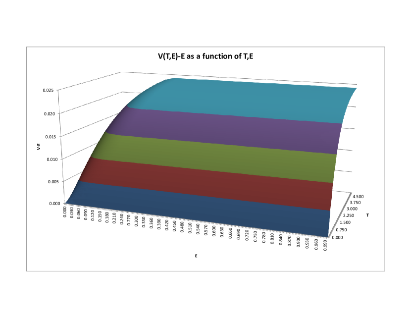
where $\tau=T-t$. The corresponding problem is solved in a relatively straightforward way by computing $\mathcal{I}_{i}$ and performing the operation $\max\left\{.,.\right\}$ explicitly, while calculating $V$ in the usual Crank-Nicolson manner. The corresponding solution is shown in Figure 12.

Figure 12 near here.

For the $T\rightarrow\infty$ limit, the time-independent maximization problem has the form

$$\begin{array}[]{c}\max\left\{\mathcal{L}\left(V\right),1-V_{E}\right\}=0,\\ V\left(0\right)=0,\end{array}$$ (152)

or, equivalently,

$$\begin{array}[]{c}\mathcal{L}\left(V\right)\left(E\right)=0,\ \ \ 0<E\leq E^{\ast},\\ V\left(E\right)=E+V\left(E^{\ast}\right)-E^{\ast},\ \ \ E^{\ast}<E<\infty,\\ V\left(0\right)=0,\\ V_{E}\left(E^{\ast}\right)=1,\\ \ V_{EE}\left(E^{\ast}\right)=0.\end{array}\$$ (153)

Here $E^{\ast}$ is not known in advance and has to be determined as part of the calculation.

It turns out that the time-independent problem can be solved analytically. Since we are dealing with a Levy process, we have

$$\mathcal{L}\left(e^{\xi E}\right)=\Psi\left(\xi\right)e^{\xi E}-\frac{\lambda_{1}\delta_{1}}{\xi+\delta_{1}}e^{-\delta_{1}E}-\frac{\lambda_{2}\delta_{2}}{\xi+\delta_{2}}e^{-\delta_{2}E},$$ (154)

where $\Psi\left(\xi\right)$ is the symbol of the pseudo-differential operator $\mathcal{L}$,

$$\Psi\left(\xi\right)=a_{2}\xi^{2}+a_{1}\xi+a_{0}+\frac{\lambda_{1}\delta_{1}}{\xi+\delta_{1}}+\frac{\lambda_{2}\delta_{2}}{\xi+\delta_{2}}.$$ (155)

Denote by $\xi_{j}$, $j=1,...,4$, the roots of the (polynomial) equation

$$\Psi\left(\xi\right)=0.$$ (156)

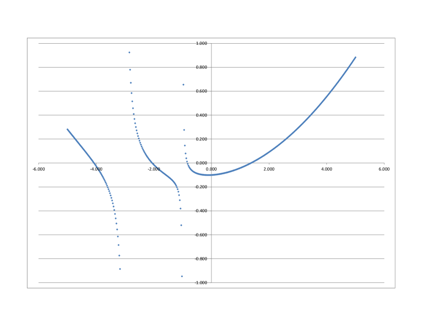
The corresponding function $\Psi\left(\xi\right)$ for a representative set of parameters is exhibited in Figure 13, which clearly shows that all roots of Eq. (156) are real.

Figure 13 near here.

Then a linear combination

$$V\left(E\right)=\sum_{j}C_{j}e^{\xi_{j}E},$$ (157)

solves the pricing problem and the boundary conditions (153) provided that

$$\left(\begin{array}[]{cccc}1&1&1&1\\ \left(\xi_{1}+\delta_{1}\right)^{-1}&\left(\xi_{2}+\delta_{1}\right)^{-1}&\left(\xi_{3}+\delta_{1}\right)^{-1}&\left(\xi_{4}+\delta_{1}\right)^{-1}\\ \left(\xi_{1}+\delta_{2}\right)^{-1}&\left(\xi_{2}+\delta_{2}\right)^{-1}&\left(\xi_{3}+\delta_{2}\right)^{-1}&\left(\xi_{4}+\delta_{2}\right)^{-1}\\ \xi_{1}e^{\xi_{1}E^{\ast}}&\xi_{2}e^{\xi_{2}E^{\ast}}&\xi_{3}e^{\xi_{3}E^{\ast}}&\xi_{4}e^{\xi_{4}E^{\ast}}\\ \xi_{1}^{2}e^{\xi_{1}E^{\ast}}&\xi_{2}^{2}e^{\xi_{2}E^{\ast}}&\xi_{3}^{2}e^{\xi_{3}E^{\ast}}&\xi_{4}^{2}e^{\xi_{4}E^{\ast}}\end{array}\right)\left(\begin{array}[]{c}C_{1}\\ C_{2}\\ C_{3}\\ C_{4}\end{array}\right)=\left(\begin{array}[]{c}0\\ 0\\ 0\\ 1\\ 0\end{array}\right).$$ (158)

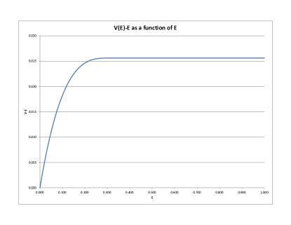
Eqs (158) should be thought of as a system of five equations for five unknowns, namely, $\left(C_{1},C_{2},C_{3},C_{4}\right)$ and $E^{\ast}$. The corresponding profile $V\left(E\right)$ is presented in Figure 14.

Figure 14 near here.

This graph shows that on the interval $\left[0,E^{\ast}\right)$ we have $V_{E}>1$. Accordingly, the coefficient $\left(1-V_{E}\right)$ in front of $d$ in Eq. (143) is negative, so that the optimal $d$ has to be zero. To put it differently, it is optimal for the bank not to pay any dividends until $E$ reaches the optimal level $E^{\ast}$. On the interval $\left(E^{\ast},\infty\right)$ we have $V_{E}>1$, so that $d$ is not determined. However, this is not particularly important, since when $E$ exceeds the optimal level $E^{\ast}$ it is optimal to pay all the excess equity in dividends. This situation occurs because we allow for infinite dividend rate, and hence lump-sum payments. When $d$ is bounded, the corresponding optimization problem is somewhat different, but can still be solved along similar lines.

Comparison of Figures 14(a) and 14(b) shows that $V\left(E\right)$ is an excellent approximation for $V\left(T,E\right)$ for longer maturities $T$.

8 Conclusions

In this paper we proposed a simple and consistent theory that enables one to examine the banking system at three levels of granularity, namely, as a whole, as an interconnected collection of banks with mutual liabilities; and, finally, as an individual bank. We demonstrated that the banking system plays a pivotal role in the monetary circuit context and is necessary for the success of the economy. Even in a relatively simple context we gained some nontrivial insights into money creation by banks and its consequences, including naturally occurring interbank linkages, as well as the role of multiple constraints banks are operating under.

The consistent quantitative description of the monetary circuit in continuous time became possible after the introduction of stochastic consumption by rentiers into the model, which enabled us to reconcile the equations with economic reality. We built a quantitative description of the monetary circuit that can be calibrated to real macro economic data which we solved mathematically. The developed framework can be further expanded by adding various sectors of the economy. It is clear that more advanced models will naturally provide deeper actionable insights, which can be used for a variety of purposes, such as setting the monetary policy, positioning banks for responsible growth, and macro investing.

At the top level, we considered the banking system as a whole, disguising therefore the structure of the banking sector and precluding investigation of defaults within it. It is hard to overestimate the importance of the quantitative approach that enables the description of a possible chain of events in the interconnected banking system in the aftermath of the crisis of 2007-2009! Hence, we expanded our analysis to the intermediate level, and demonstrated how the asset-liability balancing act creates nontrivial linkages between various banks. We used techniques developed for credit default pricing to show that these linkages can cause unexpected instabilities in the overall system. Our model can be expanded in several directions, for instance, by incorporating interbank derivatives, such as swaps, into the picture. It can provide insights into snowball effects associated with multiple simultaneous (or almost simultaneous) defaults in the banking system.

Finally, viewed at the bottom level, banks, as all other corporations, have a fiduciary obligation to responsibly maximize their profitability. Given the specifics of the banking business, such a maximization of profitability is intrinsically linked to balance sheet optimization, which is used in order to choose an optimal mix of assets and liabilities. We formulated the constrained optimization problem in the most general case, as well as its reduced version in a specific case of the equity part of the capital structure. Although simplified, the reduced problem still includes such salient elements of the equity dynamics as liquidity and solvency jumps. We then proposed a scheme to efficiently solve the corresponding constrained optimization problem.

We hope that our theory of MMC will stimulate further research along the lines suggested in the paper. In particular, to help to predict future economic crises, which naturally arise within the proposed framework.

9 Appendix A

To make our calculations in Section 6 more concrete, let us consider the case of just two banks with mutual obligations without netting, $N=2$. Additional details can be found in Itkin and Lipton (2015b).

For $0<t<T$ default boundaries have the form

$$A_{i}\leq\Lambda_{i}=\left\{\begin{array}[]{cc}R_{i}\left(L_{i}+L_{i\bar{\imath}}\right)-L_{\bar{\imath}i}\equiv\Lambda_{i}^{<},&\ t<T,\\ L_{i}+L_{i\bar{\imath}}-L_{\bar{\imath}i}\equiv\Lambda_{i}^{=},&t=T,\end{array}\right.$$ (159)

$$A_{i}\leq\tilde{\Lambda}_{i}=\left\{\begin{array}[]{cc}R_{i}\left(L_{i}+L_{i\bar{\imath}}-R_{\bar{\imath}}L_{\bar{\imath}i}\right)\equiv\tilde{\Lambda}_{i}^{<},&t<T,\\ L_{i}+L_{i\bar{\imath}}-R_{\bar{\imath}}L_{\bar{\imath}i}\equiv\tilde{\Lambda}_{i}^{=},&t=T.\end{array}\right.$$ (160)

where $\bar{\imath}=3-i$. In the $\left(A_{1},A_{2}\right)$ quadrant we have four domains

$$\mathcal{D}\left(1,1\right) = \left\{A_{1}>\Lambda_{1}^{=},\ \ \ A_{2}>\Lambda_{2}^{=}\right\},$$ (161)

$$\mathcal{D}\left(\delta_{i,1},\delta_{i,2}\right) = \left\{A_{i}>\frac{\Delta-L_{\bar{\imath}i}A_{\bar{\imath}}}{L_{\bar{\imath}}+L_{\bar{\imath}i}},\ \ \ \Lambda_{\bar{\imath}}^{<}<A_{\bar{\imath}}<\Lambda_{\bar{\imath}}^{=}\right\},\ \ \ i=1,2,$$

$$\mathcal{D}\left(0,0\right) = \left\{A_{1}>\Lambda_{1}^{<},A_{2}>\Lambda_{2}^{<}\right\}-\mathcal{D}\left(1,1\right)-\mathcal{D}\left(1,0\right)-\mathcal{D}\left(0,1\right),$$

where $\delta_{i,j}$ is the Kronecker delta, and

$$\Delta=L_{1}L_{2}+L_{1}L_{21}+L_{2}L_{12}.$$ (162)

It is clear that in $\mathcal{D}\left(1,1\right)$ both banks survive, in $\mathcal{D}\left(1,0\right)$ the first bank survives and the second defaults, in $\mathcal{D}\left(0,1\right)$ the second bank survives and the first defaults, and in $\mathcal{D}\left(0,0\right)$ both banks default. The corresponding domains are shown in Figure 15(a).

In log coordinates the domain $\mathcal{D}_{i}$ has the form

$$\mathcal{D}\left(\delta_{i,1},\delta_{i,2}\right)=\left\{X_{i}>\Theta_{i}\left(X_{\bar{\imath}}\right),0<X_{\bar{\imath}}<M_{\bar{\imath}}^{=}\right\},$$ (163)

where

$$\Theta_{i}\left(X_{\bar{\imath}}\right)=\sqrt{\frac{\sigma_{\bar{\imath}}}{\sigma_{i}}}\ln\left(\frac{\Delta-L_{\bar{\imath}i}\left(R_{\bar{\imath}}\left(L_{\bar{\imath}}+L_{\bar{\imath}i}\right)-L_{i\bar{\imath}}\right)\exp\left(\sqrt{\sigma_{\bar{\imath}}/\sigma_{i}}X_{\bar{\imath}}\right)}{\left(R_{i}\left(L_{i}+L_{i\bar{\imath}}\right)-L_{\bar{\imath}i}\right)\left(L_{\bar{\imath}}+L_{\bar{\imath}i}\right)}\right).$$ (164)

We emphasize that the domain $\mathfrak{D}_{i}$ has a curvilinear boundary which depends on the value of $A_{i}$. It is worth noting that

$$\Theta_{i}\left(0\right)=\tilde{M}_{i}^{=},\ \ \ \ \ \Theta_{i}\left(\mu_{\bar{\imath}}^{=}\right)=M_{i}^{=}.$$ (165)

The corresponding domains are shown in Figure 15(b).

Figure 15 near here.

Payoffs for different options are as follows. For the joint survival probability

$$Q\left(T,A_{1},A_{2}\right) = \boldsymbol{1}_{\left(A_{1},A_{2}\right)\in\mathcal{D}\left(1,1\right)},$$ (166)

$$Q\left(t,\delta_{i,1}\Lambda_{i}^{<}+\delta_{i,2}A_{\bar{\imath}},\delta_{i,2}\Lambda_{i}^{<}+\delta_{i,1}A_{\bar{\imath}}\right) = 0,\ \ \ i=1,2.$$

For marginal survival probabilities

$$Q_{i}\left(T,A\,_{1},A_{2}\right)=\boldsymbol{1}_{\left(A_{1},A_{2}\right)\in\mathcal{D}\left(1,1\right)+\mathcal{D}\left(\delta_{i,1},\delta_{i,2}\right)},$$ (167)

For the CDSs on the first and second bank the payoffs are as follows

$$C_{i}\left(T,A\,_{1},A_{2}\right)=\left\{\begin{array}[]{cc}0,&\left(A_{1},A_{2}\right)\in\mathcal{D}\left(1,1\right)+\mathcal{D}\left(\delta_{i,1},\delta_{i,2}\right),\\ 1-\frac{A_{i}+L_{\bar{\imath}i}}{L_{i}+L_{i\bar{\imath}}},&\left(A_{1},A_{2}\right)\in\mathcal{D}\left(\delta_{\bar{\imath},1},\delta_{\bar{\imath},2}\right),\\ 1-\frac{A_{i}+\varkappa_{\bar{\imath}}L_{\bar{\imath}i}}{L_{i}+L_{i\bar{\imath}}},&\left(A_{1},A_{2}\right)\in\mathcal{D}\left(0,0\right),\end{array}\right.$$ (168)

where the coefficients $\varkappa_{i}$ are determined from the detailed balance equations

$$A_{1}+\varkappa_{2}L_{21} = \varkappa_{1}\left(L_{1}+L_{12}\right),$$ (169)

$$A_{2}+\varkappa_{1}L_{12} = \varkappa_{2}\left(L_{2}+L_{21}\right),$$

so that

$$\varkappa_{i}=\frac{L_{\bar{\imath}}A_{i}+L_{\bar{\imath}i}\left(A_{i}+A_{\bar{\imath}}\right)}{\Delta}.$$ (170)

Finally, for the FTD the payoff has the form

$$F\left(T,A\,_{1},A_{2}\right)=\left\{\begin{array}[]{cc}0,&\left(A_{1},A_{2}\right)\in\mathcal{D}\left(1,1\right),\\ 1-\frac{A_{\bar{\imath}}+L_{i\bar{\imath}}}{L_{\bar{\imath}}+L_{\bar{\imath}i}}&\left(A_{1},A_{2}\right)\in\mathcal{D}\left(\delta_{i,1},\delta_{i,2}\right),\\ \max\left\{1-\frac{A_{1}+\varkappa_{2}L_{21}}{L_{1}+L_{12}},1-\frac{A_{2}+\varkappa_{1}L_{12}}{L_{2}+L_{21}}\right\},&\left(A_{1},A_{2}\right)\in\mathcal{D}\left(0,0\right),\end{array}\right.$$ (171)

For brevity, we consider just the calculation of the joint and marginal survival probabilities. The joint survival probability $Q\left(t,X_{1},X_{2}\right)$ solves the following terminal boundary value problem

$$Q_{t}\left(t,X_{1},X_{2}\right)+\mathcal{L}Q\left(t,X_{1},X_{2}\right)=0,$$ (172)

$$Q\left(T,X_{1},X_{2}\right)=\boldsymbol{1}_{X\in\mathcal{D}\left(1,1\right)},$$

$$Q\left(t,X_{1},0\right)=0,\ \ \ Q\left(t,0,X_{2}\right)=0,$$

The corresponding marginal survival probability for the first bank, say, $Q_{1}\left(t,X_{1},X_{2}\right)$, which is a function of both $X_{1}$ and $X_{2}$ solves the following terminal boundary value problem

$$Q_{1,t}\left(t,X_{1},X_{2}\right)+\mathcal{L}Q_{1}\left(t,X_{1},X_{2}\right)=0,$$ (173)

$$Q_{1}\left(T,X_{1},X_{2}\right)=\boldsymbol{1}_{X\in\mathfrak{D}\left(1,1\right)}+\boldsymbol{1}_{X\in\mathfrak{D}\left(1,0\right)},$$

$$Q_{1}\left(t,0,X_{2}\right)=0,$$

$$Q_{1}\left(t,X_{1},0\right)=\left\{\begin{array}[]{cc}q_{1}\left(t,X_{1}\right),&X_{1}\geq M_{1}^{\left(2\right),<},\\ 0,&X_{1}<M_{1}^{\left(2\right),<},\end{array}\right.,\ \$$ (176)

Here $q_{1}\left(t,X_{1}\right)$ is the 1D survival probability, which solves the following terminal boundary value problem

$$q_{1,t}\left(t,X_{1}\right)+\frac{1}{2}q_{1,X_{1}X_{1}}+\xi_{1}q_{1,X_{1}}=0,$$ (177)

$$q_{1}\left(T,X_{1}\right)=\boldsymbol{1}_{\left\{X_{1}>M_{1}^{\left(2\right),=}\right\}},$$

$$q_{1}\left(t,M_{1}^{\left(2\right),<}\right)=0,\ \ \$$

It is very easy to show that

$$q_{1}\left(t,X_{1}^{\prime}\right) = N\left(-\frac{M_{1}^{\left(2\right),=}-X_{1}^{\prime}-\xi_{1}\tau}{\sqrt{\tau}}\right)$$

$$-e^{-2\xi_{1}\left(X_{1}^{\prime}-M_{1}^{\left(2\right),<}\right)}N\left(-\frac{M_{1}^{\left(2\right),=}+X_{1}^{\prime}-2M_{1}^{\left(2\right),<}-\xi_{1}\tau}{\sqrt{\tau}}\right),$$

where $\tau=T-t$.

The corresponding 2D Green’s function has the form (see, e.g., Lipton 2001, Lipton and Savecu 2014):

$$\begin{array}[]{c}G\left(t,X_{1},X_{2}\right)=e^{-\left(\theta,\xi\right)t/2+\theta\cdot\left(X-X^{\prime}\right)}\bar{G}\left(t,X_{1},X_{2}\right),\\ \bar{G}\left(t,X_{1},X_{2}\right)=\frac{2e^{-\left(R^{2}+R^{\prime 2}\right)/2t}}{\bar{\rho}\varpi t}\mathop{\displaystyle\sum}\limits_{n=1}^{\infty}I_{\nu_{n}}\left(\frac{RR^{\prime}}{t}\right)\sin\left(\nu_{n}\phi\right)\sin\left(\nu_{n}\phi^{\prime}\right),\end{array}$$ (179)

where

$$\begin{array}[]{c}C=\left(\begin{array}[]{cc}1&\rho\\ \rho&1\end{array}\right),\ \ \ \ \ C^{-1}=\frac{1}{\bar{\rho}^{2}}\left(\begin{array}[]{cc}1&-\rho\\ -\rho&1\end{array}\right),\\ \theta=C^{-1}\xi,\ \ \ \bar{\rho}=\sqrt{1-\rho^{2}},\\ \varpi=\arctan\left(-\frac{\bar{\rho}}{\rho}\right),\ \ \ \ \ \nu_{n}=\frac{n\pi}{\varpi}>n,\\ R=\sqrt{\left(C^{-1}X,X\right)},\ \ \ \ \ R^{\prime}=\sqrt{\left(C^{-1}X^{\prime},X^{\prime}\right)},\\ \phi=\arctan\left(\frac{\bar{\rho}X_{1}}{-\rho X_{1}+X_{2}}\right),\ \ \ \phi^{\prime}=\arctan\left(\frac{\bar{\rho}X_{1}^{\prime}}{-\rho X_{1}^{\prime}+X_{2}^{\prime}}\right).\end{array}$$ (180)

It is clear that

$$\begin{array}[]{c}G_{X_{2}}\left(t,X_{1},0\right)=e^{-\left(\theta,\xi\right)t/2+\theta_{1}X_{1}-\theta\cdot X^{\prime}}\bar{G}_{X_{2}}\left(t,X_{1},0\right),\\ \bar{G}_{X_{2}}\left(t,X_{1},0\right)=\frac{2e^{-\left(X_{1}^{2}/\bar{\rho}^{2}+R^{\prime 2}\right)/2t}}{\varpi tX_{1}}\mathop{\displaystyle\sum}\limits_{n=1}^{\infty}\left(-1\right)^{n+1}\nu_{n}I_{\nu_{n}}\left(\frac{X_{1}R^{\prime}}{\bar{\rho}t}\right)\sin\left(\nu_{n}\phi^{\prime}\right).\end{array}$$ (181)

Substitution of these formulas in Eqs (112), (6.3) yield semi-analytical expressions for $Q$ and $Q_{1}$. The corresponding expression for $Q_{2}$ is similar.

We present $Q_{1}\left(0,X_{1},X_{2}\right)$ and the difference $q_{1}\left(0,X_{1}\right)-Q_{1}\left(0,X_{1},X_{2}\right)$ in Figures 16(a) and 16(b), respectively. These Figures show that mutual obligations significantly impact survival probabilities and other quantities of interest.

Figure 16 near here.

Figure 1: Typical solutions of LVGEs without regularization. Natural constraints are violated. Representative parameters are $a=0.225,b=0.20,c=0.4,d=0.6$. Initial conditions for subfigures 1-2, 3-4, and 5-6 are $(s_{w}=0.75,\lambda_{w}=0.8)$, $(s_{w}=0.75,\lambda_{w}=0.9)$, and $(s_{w}=0.75,\lambda_{w}=0.95)$, respectively.

Figure 2: Typical solutions of LVGEs with regularization. Natural constraints are satisfied. The same parameters and initial conditions as in Figure 1 are used; in addition, $\omega=0.005$.

Figure 3: Typical solutions of LVGEs with regularization and stochasticity. Natural constraints are satisfied; orbits are non-periodic. The same parameters and initial conditions as in Figure 2 are used; in addition, $\sigma_{s}=0.015,\sigma_{l}=0.005$.

Figure 4: Typical solutions of KEs without regularization. Natural constraints are violated. Representative parameters are $a=0.225,b=0.20,c=0.075,d=0.03,r_{L}=0.03,\nu_{f}=0.1,p=-0.0065,q=20.0,r=-5.0$. Initial conditions for subfigures 1-2, 3-4, and 5-6 are $(s_{w}=0.75,\lambda_{w}=0.8,\Gamma_{f}=0.1)$, $(s_{w}=0.75,\lambda_{w}=0.9,\Gamma_{f}=0.2)$, and $(s_{w}=0.75,\lambda_{w}=0.95,\Gamma_{f}=0.3)$, respectively.

Figure 5: Typical solutions of KEs with regularization. Natural constraints are satisfied. The same parameters and initial conditions as in Figure 4 are used; in addition, $\omega=0.005$.

Figure 6: Typical solutions of KEs with regularization and stochasticity. Natural constraints are satisfied; orbits are non-periodic. The same parameters and initial conditions as in Figure 5 are used; in addition, $\sigma_{s}=0.005,\sigma_{l}=0.005$.

Figure 7: Sketch of the Monetary Circuit. G - government, CB - central bank, PB - private banks, F - firms, H - households including rentiers and workers, NFA - non-financial assets.

Figure 8: Evolution of various quantities of interest in the non-stochastic circuit. Representative parameters and initial conditions are as follows: $\kappa_{C}=0.5,\delta_{b}b=0.5,\delta_{r}b=0.5,\delta_{f}f=0.25,\delta_{r}f=0.75,\xi_{\Delta}=0.025,\xi_{A}=0.02,r_{D}=0.02,r_{L}=0.04,\nu=0.13,\alpha_{0}=0.5,\alpha_{1}=0.5,\upsilon_{0}=-1.6,\upsilon_{1}=1.1,\upsilon_{2}=0.1,\upsilon_{0}=-0.2,a=0.05,b=0.05,c=0.075,\omega=0.005$, $C_{r}=3,D_{r}=30,L_{r}=20,D_{f}=20,L_{f}=50,K_{f}=40,K_{b}=20,s_{w}=0.7,\lambda_{w}=0.95$.

Figure 9: Credit money creation and annihilation by one commercial bank.

Figure 10: Credit money creation by two commercial banks.

Figure 11: Comparison of balance sheets of a non-financial company (subfigure a), and a representative commercial bank (subfigure b).

Figure 12: Excess value $V\left(T,E\right)-E$ viewed as a function of time to maturity $T$ and equity value $E$ for some representative parameters: $\sigma=0.25$, $\mu=0.05$, $\nu=0.10$, $\lambda_{1}=0.05$, $\delta_{1}=3.00$, $\lambda_{2}=0.02$, $\delta_{2}=1.00$.

Figure 13: Function $\Psi\left(\xi\right)$ for the same set of parameters as used in Figure 12. It is easy to see that equation $\Psi\left(\xi\right)=0$ has four roots $\xi_{1}=-4.08$, $\xi_{2}=-2.06$, $\xi_{3}=-0.84$, and $\xi_{4}=1.37$.

Figure 14: Excess value $V(T,E)-E$ viewed as a function of equity value $E$ for different times $T$(subfigure a); limiting excess value $V(\inf,E)-E$ viewed as a function of equity value $E$ (subfigure b). Subfigures (a) and (b) agree perfectly. The same parameters as in Figure 12 are used.

Figure 15: Default boundaries for two interconnected banks in the $(A_{1},A_{2})$ plane (subfigure a), and in the $(X_{1},X_{2})$ plane (subfigure b). Here $L_{1}=50,L_{1}2=10,R_{1}=0.4,L_{2}=60,L_{2}1=20,R_{2}=0.4$.

Figure 16: Marginal survival probability $Q_{1}(0,X_{1},X_{2})$ (subfigure a); decrease in marginal survival probability $q_{1}(0,X_{1})-Q_{1}(0,X_{1},X_{2})$ due to mutual liabilities between two banks (subfigure b). We use the same parameters as in Figure 15. In addition, we choose $\sigma_{1}=\sigma_{2}=0.4,\rho_{12}=0,\mu=0,T=12.5Y$.

References

- [1] Allen, F. and Babus, A., Networks in finance. In The Network Challenge: Strategy, Profit, and Risk in an Interlinked World, edited by P. Kleindorfer, Y. Wind and R. Gunther, 367–382, 2009. (Prentice Hall Professional: Upper Saddle River, NJ).
- [2] Astic, F. and Tourin, A., Optimal bank management under capital and liquidity constraints. Working paper, 2013.
- [3] Backus, D., Brainard, W., Smith, G. and Tobin, J., A model of the U.S. financial and non-financial economic behavior. Journal of Money, Credit and Banking, 1980, 12(2), 259-293.
- [4] Barbosa-Filho, N. and Taylor, L., Distributive and demand cycles in the US economy – a structuralist Goodwin model, Metroeconomica, 2006, 57, 389-411.
- [5] Baxter, W. T., Early accounting: the tally and checkerboard. The Accounting Historians Journal, 1989, 16(2), 43-83.
- [6] Bellofiore, R., Davanzati, G.F. and Realfonzo, R, Marx inside the Circuit: discipline device, wage bargaining and unemployment in a sequential monetary economy. Review of Political Economy, 2000, 12, 403-17.
- [7] Belhaj, M., Optimal dividend payments when cash reserves follow a jump-diffusion process. Mathematical Finance, 2010, 20, No. 2, 313–325.
- [8] Bernanke, B. and Blinder, Credit, money and aggregate demand. American Economic Review, 1989, 78(2), 435-439.
- [9] Birge J.R. and Judice P., Long-term bank balance sheet management: estimation and simulation of risk-factors. Journal of Banking & Finance, 2013, 37, 4711-4720.
- [10] Black, F. and Cox, J.C., Valuing corporate securities: Some effects of bond indenture provisions. Journal of Finance, 1976, 31(2), 351–367.
- [11] Blanchflower, D.G. and Oswald, A.J., The Wage Curve, 1994 (MIT Press: Cambridge, MA).
- [12] Cai, G.Q. and Lin, Y.K., Stochastic analysis of the Lotka-Volterra model for ecosystems, Physical Review E, 2004, 70, 041910.
- [13] Cantillon, R. Essai sur la Nature du Commerce en Général (1755), 2010 (Ludwig von Mises Institute: Auburn, AL).
- [14] Cassel, G., The Theory of Social Economy (1924), 1967 (A.M. Kelley Publishers: New York, NY).
- [15] Caverzasi, E. and Godin, A., Stock-flow consistent modeling through the ages. Working Paper No. 745, 2013 (The Levy Economics Institute: Annandale-on-Hudson, N.Y).
- [16] Crick, W.F., The genesis of bank deposits. Economica, 1927, 7(20), 191–202.
- [17] Dallery, T. and van Treeck, T., Conflicting claims and equilibrium adjustment processes in a stock-flow consistent macro model. Review of Political Economy, 2011, 23(2), 189 – 211.
- [18] Dalio, R., Economic Principles. Unpublished Manuscript, 2015
- [19] Davidson, P., Financial Markets, Money and the Real World, 2002 (Edward Elgar: Cheltenham).
- [20] De Carvalho, F., Mr. Keynes and the Post-Keynesians: Principles of Macroeconomics for a Monetary Production Economy, 1992 (Edward Elgar: Cheltenham).
- [21] Dempster, M.A.H., Pflug, G. and Mitra, G., Quantitative Fund Management, 2009 (Chapman & Hall / CRC: Boca Raton, FL).
- [22] Desai, M., Henry, B., Mosley, A. and Pemberton, M., A clarification of the Goodwin model of the growth cycle. Journal of Economic Dynamics and Control, 2006, 30, 2661-2670.
- [23] Diamond, D.W. and Dybvig, P.H., Bank runs, deposit insurance, and liquidity. Journal of Political Economy, 1983, 91(3), 401–419.
- [24] Domar, E., Capital Expansion, Rate of Growth, and Employment. Econometrica, 1946, 14 (2), 137–147.
- [25] Dos Santos, C. and Zezza, G., A Post-Keynesian stock-flow consistent macroeconomic growth model: preliminary results’, Working Paper No. 402, 2004 (The Levy Economics Institute: Annandale-on-Hudson, N.Y).
- [26] Dos Santos, C. and Zezza, G. 2006, Distribution and growth in a Post-Keynesian stock-flow consistent model. In Economic Growth and Distribution: on the Nature and Causes of the Wealth of Nations, edited by N. Salvadori, 2006 (Edward Elgar: Cheltenham).
- [27] dos Reis S.G. and Martins, E., Planejamento do Balanço Bancário: Desenvolvimento de um Modelo Matemático de Otimização do Retorno Econômico Ajustado ao Risco. Revista Contabilidade & Finanças FIPECAFI - FEA - USP, 2001, 15, 58-80.
- [28] Egloff, D., Leippold, M. and Vanini, P., A simple model of credit contagion. Journal of Banking and Finance, 2007, 31, 2475–2492.
- [29] Eisenberg, L. and Noe, T.H., Systemic risk in financial systems. Management Science, 2001, 47(2), 236–249.
- [30] Fama, E., What’s different about banks? Journal of Monetary Economics, 1985, 15, 29–39.
- [31] Federal Reserve Board, The Federal Reserve System: Purposes and Functions, 9th ed., 2005 (Board of Governors of the Federal Reserve System: Washington, DC).
- [32] Flaschel, P., The Macrodynamics of Capitalism. Elements for a Synthesis of Marx, Keynes and Schumpeter, 2010 (Springer: Heidelberg).
- [33] Fontana, G. and Realfonzo, R., (eds.), The Monetary Theory of Production, 2005 (Palgrave: New York).
- [34] Franke, R., Flaschel, P. and Proaño, C.R., Wage–price dynamics and income distribution in a semi-structural Keynes–Goodwin model. Structural Change and Economic Dynamics, 2006, 17(4), 452-465.
- [35] Freixas, X., Parigi, B. and Rochet, J.C., Systemic risk, interbank relations, and liquidity provision by the central bank. Journal of Money, Credit and Banking, 2000, 32, 611–638.
- [36] Friedman, M., The Optimum Quantity of Money and Other Essays, 1969 (Transaction Publishers: Piscataway, NJ)
- [37] Friedman, M., and Schwartz, A., Monetary Trends in the United States and United Kingdom: Their Relation to Income, Prices, and Interest Rates, 1867-1975, 1982 (University of Chicago Press: Chicago, IL).
- [38] Godley, W., Money and credit in a Keynesian model of income determination. Cambridge Journal of Economics, 1999, 23(4), 393-411.
- [39] Godley, W. and Lavoie, M., Monetary Economics: An Integrated Approach to Credit, Money, Income, Production and Wealth, 2007 (Palgrave Macmillan: London).
- [40] Goodwin, R. M. 1967 A growth cycle. In Socialism, Capitalism and Economic Growth, edited by C.H. Feinstein, 54-58, 1967. (Cambridge University Press: Cambridge).
- [41] Gnos, C., Circuit theory as an explanation of the complex real world. In: Modern Theories of Money: The Nature and Role of Money in Capitalist Economies, edited by L.-P. Rochon & S. Rossi, 2003 (Edward Elgar: Cheltenham).
- [42] Graeber, D., Debt: The First 5000 Years, 2011 (Melville House: Brooklyn, NY)
- [43] Grasselli, M.R. and Costa Lima, B., An analysis of the Keen model for credit expansion, asset price bubbles and financial fragility. Mathematics and Financial Economics, 2012, 6(3), 191-210.
- [44] Graziani, Augusto, The Monetary Theory of Production, 2003 (Cambridge University Press: Cambridge).
- [45] Guttentag, J. M. and Lindsay, R., The uniqueness of commercial banks. Journal of Political Economy, 1968, 76(5), 991–1014.
- [46] Hahn, A.C., Volkswirtschaftliche Theorie des Bankkredits, 1920 (J.C.B.Mohr: Tübingen).
- [47] Halaj, G., Optimal Balance Sheet Structure of a Bank: Bank Reactions to Stressful Market Conditions. European Central Bank Working Paper, 2012.
- [48] Haldane, A. and May, R., Systemic risk in banking ecosystems. Nature, 2011, 469(7330), 351–355.
- [49] Harrod, R.F., An Essay in Dynamic Theory. The Economic Journal, 1939, 49 (193), 14–33.
- [50] Harvie, D., Kelmanson, M. and Knapp, D., A dynamical model of business-cycle asymmetries: extending Goodwin. Economic Issues, 2007, 12, 53-92.
- [51] Heffernan, S., Modern Banking in Theory and Practice, 1996 (John Wiley and Sons: Chichester).
- [52] Hein, E., Interest, Debt and Capital Accumulation - A Kaleckian Approach. International Review of Applied Economics, 2006, 20(3), 337-52.
- [53] Howe, R.H., The Evolution of Banking; A Study of the Development of the Credit System, 1915 (C.H. Kerr & Company: Chicago, IL).
- [54] Huu A.N. and Costa-Lima, B. Orbits in a stochastic Goodwin-Lotka-Volterra model. Working Paper, 2014.
- [55] Hurd, T.R., Contagion! The Spread of Systemic Risk in Financial Networks, 2015 (Springer: Berlin, Heidelberg, New York).
- [56] Ingham, G.K., The Nature of Money, 2004 (Polity Press: Cambridge).
- [57] Itkin, A. and Lipton, A., Efficient solution of structural default models with correlated jumps and mutual obligations. International Journal of Computer Mathematics, 2015a.
- [58] Itkin, A. and Lipton, A., Structural default model with mutual obligations. Working Paper, arXiv.org, 2015b.
- [59] Jevons, W.S., Money and the Mechanism of Exchange, 1875 (Macmillan: London).
- [60] Kalecki, M., Essays in the Theory of Economic Fluctuations (1939). In: Collected Works of Michael Kalecki,. Vol. I; Capitalism, Business and Full Employment, edited by J. Osiatynski, J. (2007). 235-252, 2007 (Clarendon Press: Oxford).
- [61] Kalecki, M. Selected Essays on the Dynamics of the Capitalist Economy 1933-1970, 1971 (Cambridge University Press, Cambridge).
- [62] Keen, .S., Finance and economic breakdown: modelling Minsky’s Financial Instability Hypothesis. Journal of Post Keynesian Economics, 1995, 17, 607-635.
- [63] Keen, S., A monetary Minsky model of the Great Moderation and the Great Recession. Journal of Economic Behavior & Organization, 2013, 86, 221-235.
- [64] Keen, S., Secular stagnation and endogenous money. Real World Economics Review, 2014, 66, 2-11.
- [65] Keynes, J.M., A Treatise on Money, 1930 (Macmillan: London).
- [66] Keynes, J.M., The General Theory of Employment, Interest, and Money, 1936 (Macmillan: London).
- [67] Klein, M.A., A theory of the banking firm. Journal of Money, Credit and Banking, 1971, 3, 205–218.
- [68] Knapp, G.F., Staatliche Theorie des Geldes, 1905 (Duncker & Humblot: Leipzig).
- [69] Kocherlakota N.R., Money is memory. Journal of Economic Theory, 1998, 81, 232–51.
- [70] Kodera, J. and Vosvrda, M., Goodwin’s Predator-Prey Model with Endogenous Technological Progress. Working Paper. Institute of Economic Studies, Faculty of Social Sciences, Charles University in Prague, 2007.
- [71] Kusy, M.I. and Ziemba, W.T., A bank asset and liability management model. Operations Research, 1986, 34(3), 356-376.
- [72] Ladley, D., Contagion and risk-sharing on the inter-bank market. Journal of Economic Dynamics and Control, 2013, 37(7), 1384–1400.
- [73] Lavoie, M., Endogenous money in a coherent stock-flow framework. Working Paper no. 325, 2001 (The Levy Economics Institute: Annandale-on-Hudson, N.Y).
- [74] Lavoie, M. Circuit and Coherent Stock-Flow Accounting. In Money, Credit and the Role of the State, edited by R. Arena and N. Salvadori, 2004 (Ashgate: Aldershot).
- [75] Lavoie, M. and Godley, W., Kaleckian growth models in a stock and flow monetary framework: a Kaldorian view. Journal of Post Keynesian Economics, 2001-2002, 24(2), (Winter), 277-312.
- [76] Law, J., Money and Trade Considered with a Proposal for Supplying the Nation with Money, 1705 (R. & A. Foulis: Glasgow).
- [77] Le Heron, E., Financial crisis and banking behavior in a post-Keynesian stock-flow consistent model. Working Paper, CEPN, 2009.
- [78] Le Heron, E. and Mouakil, T., A post Keynesian stock-flow consistent model for the dynamic analysis of monetary policy shock on banking behavior. Metroeconomica, 2008, 59(3), 405-40.
- [79] Leitner, Y., Financial networks: contagion, commitment, and private sector bailouts. Journal of Finance, 2005, 60, 2925–2953.
- [80] Lipton, A., Mathematical Methods for Foreign Exchange: a Financial Engineer Approach, 2001 (World Scientific: Singapore).
- [81] Lipton, A., Evauating the latest structural and hybrid models for credit risk. Conference Presentation. Global Derivatives, Barcelona, May 21st, 2003.
- [82] Lipton, A. and Savescu, I., Pricing credit default swaps with bilateral value adjustments. Quantitative Finance, 2014, 14(1), 171-188.
- [83] Lipton, A. and Sepp, A., Credit value adjustment for credit default swaps via the structural default model. Journal of Credit Risk, 2009, 5(2), 123–146.
- [84] Lotka, A.Y., Elements of Physical Biology, 1925 (Williams and Wilkins: Baltimore).
- [85] Macleod, H.D., The Theory and Practice of Banking, in 2 volumes (1855–6), 1905 (Longman, Greens and Co: London).
- [86] Marshall, A., Report by the Gold and Silver Commission of 1887.
- [87] Marshall, A.W., and Olkin, I., A multivariate exponential distribution. Journal of American Statistical Association, 1967, 2, 84-98.
- [88] Marx, K., Das Kapital: Kritik der Politischen Oekonomie, 1867 (Verlag von Otto Meissner: Hamburg).
- [89] McLeay, M., Radia, A. and Thomas, R., Money in the modern economy: An introduction. Bank of England Quarterly Bulletin, Q1, 2014.
- [90] Mehrling, P., Modern money: fiat or credit? Journal of Post Keynesian Economics, 2000, 22, 397–406.
- [91] Merton, R., On the pricing of corporate debt: the risk structure of interest rates. Journal of Finance, 1974, 29, 449–470.
- [92] Mitchell-Innes, A., The credit theory of money. Banking Law Journal, 1914, 31 151–68.
- [93] Minsky, H.P., John Maynard Keynes, 1975 (Columbia University Press: NewYork, NY).
- [94] Minsky, H.P., The Financial Instability Hypothesis: an interpretation of Keynes and an alternative to “standard” theory. Nebraska Journal of Economics and Business, 1977, 16(1), 5–16.
- [95] Minsky, H.P., Stabilizing an unstable economy, 1986 (Yale University Press: New Haven and London).
- [96] Moore, B.J., Horizontalists and Verticalists: The Macroeconomics of Credit Money, 1988 (Cambridge University Press: Cambridge).
- [97] Moore, B.J. Shaking the Invisible Hand: Complexity, Endogenous Money and Exogenous Interest Rates, 2006 (Palgrave Macmillan: Houndmills, UK and New York).
- [98] Mukuddem-Petersen, J. and Petersen, M.A., Bank management via stochastic optimal control. Automatica, 2006, 42(8), 1395-1406.
- [99] Nakamoto, S., Bitcoin: A Peer-to-Peer Electronic Cash System. Working Paper, www.bitcoin.org, 2009.
- [100] Parguez, A. and Secareccia, M., The credit theory of money: the monetary circuit approach. In: What is Money?, edited by J. Smithin, 2000 (Routledge: London).
- [101] Pastor-Satorras, R. and Vespignani, A., Epidemic spreading in scale-free networks. Physical Review Letters, 2001, 86, 3200–3203.
- [102] Petty, W., The Economic Writings of Sir William Petty, Vol. I, 1899 (Cambridge University Press: Cambridge).
- [103] Phillips, A.W., The relation between unemployment and the rate of change of money wage rates in the United Kingdom, 1861–1957. Economica, 1958, 25(100), 283–299.
- [104] Piketty, T., Capital in the Twenty-First Century, 2013 (Belknap Press of Harvard University Press: Cambridge, MA).
- [105] Quesnay, F., Physiocratie (1759). Edition de J. Cartellier, 1991 (Flammarion: Paris).
- [106] Realfonzo, R., Money and Banking, 1998 (Edward Elgar: Cheltenham).
- [107] Rochet, J.-C. and Tirole, J. Interbank lending and systemic risk. Journal of Money, Credit and Banking, 1996, 28(4), 733–762.
- [108] Sawyer, M., Macro-economics in Question: The Keynesian-Monetarist Orthodoxies and the Kaleckian Alternative, 1982 (M.E. Sharpe: Armonk, NY).
- [109] Samuelson, P. and Nordhaus, W., Economics, 1995. (McGraw-Hill: New York, NY).
- [110] Saving, T.R., A theory of the money supply with competitive banking. Journal of Monetary Economics, 1977, 3, 289–303.
- [111] Say, J.-B., Traité d’economie politique, 1803 (Deterville: Paris).
- [112] Sbordone, A., Tambalotti, A.,Rao, K. and Kieran Walsh, K. (2010), Policy analysis using DSGE models: an introduction. FRBNY Economic Policy Review, 2010, 16 (2), 23-43.
- [113] Schlesinger K., Theorie der Geld- und Kreditwirtschaft, 1914 (Duncker & Humblot: Berlin).
- [114] Schumpeter, J., Theorie der wirtschaftlichen Entwicklung, 1912 (Duncker & Humblot: Berlin).
- [115] Schumpeter J., Das Wesen des Geldes, 1970 (Vandenhoek & Ruprecht: Göttingen).
- [116] Sealey, C. and Lindley, J. T., Inputs, outputs and a theory of production and cost at depositary financial institutions. Journal of Finance, 1977, 32, 1251–1266.
- [117] Secareccia, M. Pricing, investment and the financing of production within the framework of the monetary circuit: some preliminary evidence. In: Modern Theories of Money: The Nature and Role of Money in Capitalist Economies, edited by L.-P. Rochon and S. Rossi, 2003 (Edward Elgar: Cheltenham).
- [118] Selgin, G. and White, L., The evolution of a free banking system. Economic Inquiry, 1987, 25, 439–457.
- [119] Selyutin, V. and Rudenko, M., Mathematical Model of Banking Firm as Tool for Analysis, Management and Learning. Working Paper, 2013.
- [120] Smith, A. An Inquiry into the Nature and Causes of the Wealth of Nations, 1776, 1977 (The University of Chicago Press: Chicago, IL).
- [121] Soddy, F., The Role of Money, 1934 (Elkin Mathews & Marrot: London).
- [122] Solow, R.M., Goodwin’s Growth Cycle; Reminiscence and Rumination. In Nonlinear and Multi-sectoral Macrodynamics, edited by K. Velupillai, 1990 (Macmillan: London).
- [123] Sraffa, P., Production of Commodities by Means of Commodities, 1960 (Cambridge University Press: Cambridge).
- [124] Steinbacher, M., Steinbacher, M., and Steinbacher, M., Banks and their contagion potential: how stable is banking system? In Artificial Economics and Self Organization, edited by S. Leitner and F. Wall, 2014, 161–175 (Springer: Berlin).
- [125] Stiglitz, J., Economics, 2nd ed., 1997 (W.W. Norton: New York).
- [126] Taksar, M., Optimal risk/dividend distribution control models: applications to insurance. Mathematical Methods of Operations Research, 2000, 1, 1-42.
- [127] Taylor, L., Growth, cycles, asset prices, and finance. Metroeconomica, 2012, 63(1), 40–63.
- [128] Tobin, J., Commercial banks as creators of ”money”. In Banking and Monetary Studies, edited by D. Carson, 408-419, 1963 (Comptroller of the Currency: Washington).
- [129] Tobin, J., A general equilibrium approach to monetary theory. Journal of Money, Credit and Banking, 1969, 1, 15-29.
- [130] Tobin, J., Money and Finance in the Macroeconomic Process. Journal of Money, Credit and Banking, 1982, 14(2), 171–204.
- [131] Tobin, J. and Golub, S., Money, Credit, and Capital, 1998 (Irwin McGraw-Hill: Boston, MA).
- [132] Van Treek, T., A synthetic stock-flow consistent macroeconomic model of financialisation. Working Paper 6/2007, Institut for Macroökonomie und Konjuncturforschung, Düsseldorf, 2007.
- [133] Veneziani, R. and Mohun, S., Structural stability and Goodwin’s growth cycle. Structural Change and Economic Dynamics, 2006, 17.4, 437-451.
- [134] Volterra, V., Leçons sur la Théorie Mathématique de la Lutte por la Vie, 1931 (Gauthier-Villar: Paris).
- [135] von Mises, L., Theorie des Geldes und der Umlaufsmittel, 1924 (Duncker & Humblot: Berlin).
- [136] Wagner, W., Diversification at financial institutions and systemic crises. Journal of Financial Intermediation, 2010, 19(3), 373–386.
- [137] Webber, L. and Willison, M., Systemic capital requirements. Tech. Rep. 436, Bank of England, 2011.
- [138] Werner, R.A., New paradigm in macroeconomics, 2005 (Palgrave Macmillan: Basingstoke).
- [139] Werner, R.A., Can banks individually createmoney out of nothing? - The theories and the empirical evidence. International Review of Financial Analysis, 2014, 36, 1–19.
- [140] Wicksell, K., Lectures on Political Economy, 1935. (Routledge: London).
- [141] Wolf, M., Strip private banks of their power to create money. Financial Times, Apr. 24, 2014.
- [142] Zezza, G. and Dos Santos, C.H., The role of monetary policy in post-Keynesian stockflow consistent macroeconomic growth models. In Central Banking in the Modern World: Alternative Perspectives, edited by M. Lavoie and M. Seccareccia, 181-208, 2004 (Edward Elgar: Cheltenham).